Model-based Clustering

Bettina Grün Mixture models extend the toolbox of clustering methods available to the data analyst. They allow for an explicit definition of the cluster shapes and structure within a probabilistic framework and exploit estimation and inference techniques available for statistical models in general. In this chapter an introduction to cluster analysis is provided, model-based clustering is related to standard heuristic clustering methods and an overview on different ways to specify the cluster model is given. Post-processing methods to determine a suitable clustering, infer cluster distribution characteristics and validate the cluster solution are discussed. The versatility of the model-based clustering approach is illustrated by giving an overview on the different areas of applications. finite mixture model, heuristic clustering, infinite mixture model, unsupervised learning Bettina Grün
Institut für Angewandte Statistik
Johannes Kepler Universität Linz
Altenbergerstraße 69
4040 Linz, Austria
E-mail:
URL: http://ifas.jku.at/gruen/

1 Introduction

Cluster analysis – also known as unsupervised learning – is used in multivariate statistics to uncover latent groups suspected in the data or to discover groups of homogeneous observations. The aim thus is often defined as partitioning the data such that the groups are as dissimilar as possible and that the observations within the same group are as similar as possible. The groups composing the partition are also referred to as clusters.

Cluster analysis can be used for different purposes. It can be employed (1) as an exploratory tool to detect structure in multivariate data sets such that the results allow to summarise and represent the data in a simplified and shortened form, (2) to perform vector quantisation and compress the data using suitable prototypes and prototype assignments and (3) reveal a latent group structure which corresponds to unobserved heterogeneity. A standard statistical textbook on cluster analysis is for example Everitt et al. (2011).

Clustering is often referred to as an ill-posed problem which aims at revealing interesting structures in the data or deriving a useful grouping of the observations. However, specifying what is interesting or useful in a formal way is challenging. This complicates the specification of suitable criteria for selecting a clustering method or a final clustering solution. Hennig (2015) also emphasises this point. He argues that the definition of what the true clusters are depends on the context and the clustering aim. Thus there does not exist a unique clustering solution given the data, but different clustering aims imply different solutions and analysts should in general be aware of the ambiguity inherent in cluster analysis and thus transparently point out their clustering aims together with their solutions obtained.

At the core of cluster analysis is the definition of what a cluster is. This can be achieved by defining the characteristics of the clusters which should emerge as output from the analysis. Often these characteristics can only be informally defined and are not directly useful to select a suitable clustering method. In addition also some notion on the total number of clusters suspected or the expected size of clusters might be needed to characterise the cluster problem. Furthermore, domain knowledge is important to decide on a suitable solution, in the sense that the derived partition consists of interpretable clusters which have practical relevance. However, domain experts are often only able to assess the suitability of a solution once they are confronted with a grouping but are unable to provide clear characteristics of the desired clustering beforehand.

Model-based clustering can help in the application of cluster analysis by requiring the analyst to formulate the probabilistic model which is used to fit the data and thus making the aims and the cluster shapes aimed for more explicit than what is generally the case if heuristic clustering methods are used. The use of mixture models for clustering is also discussed in the general textbooks on mixture models by McLachlan and Peel (2000a) and Frühwirth-Schnatter (2006). In addition several review articles on model-based clustering are available including Stahl and Sallis (2012) and McNicholas (2016b) as well as the monograph on mixture model-based classification by McNicholas (2016a).

In the following heuristic clustering methods are described and their relation to Gaussian mixture modelling is elaborated. After discussing the specification of the clustering problem, strategies for selecting a suitable mixture model together with the appropriate clustering base are pointed out in Section 2. The post-processing methods given a fitted model are outlined in Section 3 which allow to obtain an identified model, derive a partition of the data, characterise the cluster distributions, gain insights through suitable visualisations and validate the clustering. Model-based clustering has been used in a range of different applications where also methodological advances have emerged from. Some important areas are discussed in detail in Section 4.

1.1 Heuristic clustering

Heuristic clustering methods are based on the definition of similarities or dissimilarities between observations and groups of observations. These are used as input to the different cluster algorithms proposed. In general two main clustering strategies are distinguished: hierarchical clustering and partitioning clustering.

In hierarchical clustering a nested sequence of partitions is constructed. This is accomplished either in a bottom-up (agglomerative) or a top-down (divisive) approach. In bottom-up or agglomerative clustering, each observation starts in its own cluster and in each step two clusters are merged until all observations are contained in one single cluster. By contrast top-down or divisive clustering starts with a single cluster and in each step splits one cluster into two. A greedy search strategy is employed where in each single step the optimal one-step ahead decision is made. However, this does not imply that any of the intermediate cluster solutions obtained is optimal.

In order to obtain an optimal partition of $n$ observations $\mathbf{y}=(y_{1},\ldots,y_{n})$ for a given number of clusters $G$, a partitioning cluster algorithm needs to be used. The $k$-means algorithm aims at finding the partition ${\cal P}$ which minimises the within-cluster sum-of-squares,

$$\arg\min_{{{\cal P}}}\sum_{g=1}^{G}\sum_{i\in{{\cal C}}_{g}}\sum_{j\in{{\cal C}}_{g}}\|{y}_{i}-{y}_{j}\|^{2},$$

where ${{\cal C}}_{g}$ is the set of observations assigned to group $g$ by the partition ${{\cal P}}$ and $\|\cdot\|$ denotes the Euclidean distance. The solution to this objective function can also be obtained by solving the following optimisation problem

$$\arg\min_{{{\cal P}}}\sum_{g=1}^{G}\sum_{i\in{{\cal C}}_{g}}\|{y}_{i}-{\bar{y}_{g}}\|^{2},$$

where the cluster centroid ${\mu}_{g}$ is equal to $\bar{y}_{g}$ which is given by

$$\bar{y}_{g} =\frac{1}{n_{g}}\sum_{i\in{{\cal C}}_{g}}{y}_{i},$$

with $n_{g}$ the number of observations in group $g$. Note that if the partition is restricted to contain only non-empty elements, $G$ is necessarily finite for a finite sample of size $n$, but if the partition ${\cal P}$ may also contain empty groups $G=\infty$ is also possible. This observation similarly holds also for the mixture models subsequently considered. For mixture models finite or infinite values for $G$ might be used to represent the theoretic data-generating process. However, the induced partitions will consist of a finite number of groups for finite samples. Also the number of components with observations assigned will be finite for finite samples.

Extension of the $k$-means algorithm to alternative dissimilarity measures than the squared Euclidean distance have been proposed leading to $k$-centroid cluster analysis (Leisch, 2006). These variants can also be used for multivariate data where variables are collected on different scale levels and which require specific dissimilarity measures. For example for asymmetric binary data the Jaccard distance or Jaccard coefficient (Jaccard, 1912) has been proposed as suitable dissimilarity measure because it disregards joint zeros (see, for example, Kaufman and Rousseeuw, 1990, p. 26).

1.2 From $k$-means to Gaussian mixture modelling

If finite mixtures of multivariate Gaussian distributions are used for model-based clustering, a probabilistic distribution is specified which is used as a data-generating process for the observed data. In particular it is assumed that the data in each group or cluster is generated from a multivariate Gaussian distribution and the combined data stems from a convex combination of multivariate Gaussian distributions. This distribution used in Gaussian mixture modelling is given by

$$\sum_{g=1}^{G}\eta_{g}\phi({y}|{\mu}_{g},\Sigma_{g}),$$

where $\phi(\cdot|\mu,\Sigma)$ is the pdf of the multivariate Gaussian distribution with mean $\mu$ and covariance matrix $\Sigma$, corresponding to the cluster distribution, and $\eta_{g}$ are the cluster sizes with $\eta_{g}\geq 0,\sum_{g=1}^{G}\eta_{g}=1.$ The parameters $\theta$ in this model are the cluster sizes $\eta_{g}$, and the cluster-specific parameters consisting of the cluster means $\mu_{g}$ and the cluster covariance matrices $\Sigma_{g}$ for $g=1,\ldots,G$.

This model class can be seen as a generalisation of $k$-means clustering. Define $\mathbf{z}=(z_{1},\ldots,z_{n})$, where $z_{i}\in\{1,\ldots,G\}$ is the cluster membership of observation $i$. The $k$-means clustering solution can also be obtained by maximising the classification likelihood $p(\mathbf{y}|\mathbf{z},\theta)$ of a finite mixture of multivariate Gaussian distributions with identical isotropic covariance matrices $\Sigma_{g}=\sigma^{2}I$, where $I$ is the identity matrix, and equal weights $\eta_{g}=1/G$ with respect to the mixture parameters $\theta$ and the cluster memberships $\mathbf{z}$:

$$\sum_{i=1}^{n}\frac{1}{G}\phi(y_{i}|\mu_{z_{i}},\sigma^{2}I).$$

This implies that quite specific cluster shapes are implicitly imposed when using $k$-means clustering, namely that the clusters are spherical with equal variability in each dimension. In such a situation it is important to define a suitable scaling for each of the dimensions because the $k$-means solution treats the variability in each of the dimensions equally and the obtained solution therefore is not invariant with respect to the scaling of the variables. A data-driven approach to achieve this is often to standardise the data. This, however, is problematic if (1) extreme, outlying observations are present in the data and (2) the cluster structure is not equally strong in all dimensions leading to different between-cluster dissimilarities in the different dimensions. The dissimilarities in dimensions containing strong cluster structure are attenuated by the standardisation and thus standardisation deteriorates the obtained cluster solution. In addition the application of $k$-means favours clusters of the same size and volume. Thus making this relationship between Gaussian mixture models and $k$-means clustering explicit allows to gain insights into the implicit assumptions imposed when $k$-means clustering is used. The notion that heuristic clustering methods impose less assumptions than model-based clustering is thus clearly in error. Rather users are often less aware of the assumptions implicitly imposed when using heuristic methods.

Extending the $k$-means approach to allow for arbitrary covariance matrices in the clusters leads to model-based clustering using finite mixtures where the classification likelihood $p(\mathbf{y}|\mathbf{z},\theta)$ instead of the observed likelihood $p(\mathbf{y}|\theta)$ is maximised (Scott and Symons, 1971; Symons, 1981; McLachlan, 1982; Celeux and Govaert, 1992). In this case the parameters of the mixture model as well as the cluster memberships are estimated, implying that the number of quantities to be estimated grows with the number of observations. Under these conditions maximum likelihood estimates have been shown to be asymptotically biased (Bryant and Williamson, 1978).

The classification maximum likelihood approach can be implemented in two different ways: either excluding the cluster sizes $\bm{\eta}=(\eta_{1},\ldots,\eta_{G})$ from the likelihood or including $\bm{\eta}$ in the likelihood. The first case corresponds to implicitly assuming that they are all equal, while the second case can be seen as adding a penalty term to the classification likelihood. Maximising the classification likelihood instead of the observed likelihood has the advantage that the derived solution potentially is better suited for the clustering context and that iterative methods for model estimation such as the expectation-maximisation (EM) algorithm converge faster. Biernacki et al. (2003) thus consider to initialise the ordinary EM algorithm by first using several runs of the so-called classification EM, which implements an EM algorithm for maximising the classification likelihood, and selecting the best solution detected.

Applications of Gaussian mixture modelling are widespread and often this model class is used as the basic model for clustering metric multivariate data if $k$-means clustering is not flexible enough. Recent exemplary applications of Gaussian mixture modelling are, among many others, Kim et al. (2014) in hydrology who cluster a multivariate data set of hydrochemical measurements from groundwater samples to separate anthropogenic and natural groundwater groups. Perera and Mo (2016) used Gaussian mixture models in ocean engineering to understand marine engine operating regions as part of the ship energy efficiency management plan. In environmental science, Skakun et al. (2017) used Gaussian mixture models to determine a data-driven classification method to distinguish winter crop from spring and summer crop.

Compared to $k$-means clustering Gaussian mixture modelling has several advantages. The model explicitly allows for clusters of different siz and clusters of different volume. In addition, the clusters are independent of the scaling used for the variables (except for potential numerical issues). This flexibility comes with several drawbacks. The likelihood is unbounded for the general Gaussian mixture model and spurious solutions might emerge. Assuming a one-to-one mapping between clusters and components in the mixture model might lead to counter-intuitive clustering solutions, because (a) several components form a single mode and (b) observations are not assigned to the cluster where the component mean is closest in Euclidean space due to different component-specific covariance matrices. Finally, the fitted model might rather correspond to a semi-parametric estimation of the data distribution, than represent a useful clustering model.

Thus specification of a suitable model (see Subsection 2) and the use of appropriate post-processing techniques, discussed in Subsection 3), are essential to reach a cluster solution that is useful and meets the stated clustering aims.

1.3 Specifying the clustering problem

Hennig and Liao (2013) claim that “there are no unique ‘true’ or ‘best’ clusters in a data set”, rather it needs to be defined by the user who applies clustering methods what a cluster is. In general this consists of specifying the characteristics of a cluster regarding size and shape and how clusters are assumed to differ. This constitutes essential information in order to assess which observations form a cluster and which belong to different clusters. These decisions need to be made regardless of whether a model-based approach or a heuristic approach to clustering is employed. However, using a model-based approach makes these decisions in general more explicit. The specified model clearly indicates what cluster distributions are considered. Furthermore, in a model-based approach model selection and evaluation are based on statistical inference methods. This allows to recast the problem of choosing a suitable number of clusters as a statistical model selection problem and adds the possibility to rigorously assess uncertainty.

Different notions of what defines a cluster have been proposed and common examples of such cluster characteristics are described in the following consisting of compactness, density-based levels, connectedness and functional similarity. For illustration, 2-dimensional scatter plots of data where a clear cluster structure regarding these notions is present are used.

Compactness. A cluster is characterised by points being close to each other. Separation between observations indicates that they stem from different clusters. In this case the cluster centroid is a useful prototype for all observations in the cluster. Often the notion of compactness is used to derive a cluster solution assuming that all clusters have similar levels of compactness. This implies that all clusters have a comparable volume and that the cluster centroids equally well represent observations in their clusters. The $k$-means algorithm minimises the within-cluster sum-of-squares which can be seen as a measure of compactness and thus explicitly tries to address this clustering notion. In hierarchical clustering some linkage methods, i.e., distance definitions between groups of observations, also lead to solutions with high compactness, such as complete linkage.

Density-based levels. Areas in the observation space where observations frequently occur are referred to as density clusters. This cluster concept in general is used for continuous data. In contrast to the compactness notion clusters might have different volumes and arbitrary shapes, i.e., also non-convex shapes, are possible. However, this also implies that the centroids – a concept which might even not be well defined for non-convex clusters – do not equally well represent their assigned observations. Furthermore, new observations might be hard to assign to a cluster if they occur in regions not identified as cluster regions, i.e., assigning any (new) observations to one of the clusters might not be straightforward and unambiguous. Cluster methods which are based on an estimate of the data density and determine connected components in a density level set try to explicitly address this cluster notion (Azzalini and Menardi, 2014; Scrucca, 2016).

Connectedness. A cluster is defined by a friends-of-friends strategy. Observations are assigned to the same cluster if they are close to each other or if they are linked by other observations also assigned to the cluster. This implies that arbitrary cluster shapes are possible. However, no further structure than provided by the data itself is imposed indicating that solutions might be quite data-dependent and variable. Also characterising a cluster through a centroid or a prototype might be impossible. Some linkage methods used in hierarchical clustering favour this kind of solutions, such as single-linkage where a chaining phenomenon occurs.

Functional similarity. Observations are assigned to the same cluster if they share a common functional relationship between the variables in the different dimensions. For example, one variable might be seen as the dependent and the others as independent ones leading to a regression setting. Functional similarity then implies that the regression coefficients are similar within clusters, but differ across clusters. Network data represent another data setting where functional similarity might serve as notion for constructing clusters. In this case groups are for example formed by joining observations which have a similar linking behaviour to other observations.

Figure 1: Illustration of clustering concepts: (a) compact clusters (on the left); (b) density-based clusters (in the middle); (c) connected clusters or clusters sharing a functional relationship (on the right).

Figure 1 illustrates these different clustering concepts using three data sets containing two-dimensional metric data. The same data is also shown in Figure 2 where the information on the cluster membership of each observation is also included using different colours and numbers for the data points. The scatter plot on the left visualises a data set where the clusters are compact, i.e., they have a similar level of compactness and shape and are very well separated. This is the easiest case for clustering where most of the clustering methods employed should be able to detect the correct cluster structure. The scatter plot in the middle shows a data set where clusters correspond to high density levels and can still be represented by a cluster centroid, but differ in their level of compactness. In contrast to $k$-means, model-based clustering allows to account for these differences in compactness and to better extract the true cluster structure. The data set given in the scatter plot on the right illustrates the case where clusters can easily be identified using the connectedness concept. In addition these connected clusters might be identifiable by imposing cluster-specific functional relationships between the values on the $x$- and the $y$-axis and also by assuming that cluster sizes vary with the value of $x$. If heuristic clustering methods are used for the data set on the right, these need to be able to detect clusters based on connectedness.

If $k$-means is used to cluster the three data sets, good performance is expected for the first two which are based on the compactness and density-based concepts for clusters. $k$-means is expected to perform badly on the third data set and not to be able to detect the true cluster structure. The potential performance of $k$-means clustering on these data sets is investigated in Section 3.5. The quality of the true clustering solutions is visualised in Figure 3 using a silhouette plot based on the Euclidean distance. This indicates how $k$-means clustering might potentially perform. In addition, a silhouette-type plot is also used to illustrate how model-based clustering methods might perform on these three artificial data sets. The conditional probabilities of cluster memberships are determined based on suitable mixture models fitted using maximum likelihood estimation. These are then split by the true cluster memberships of the observations and visualised in Figure 5.

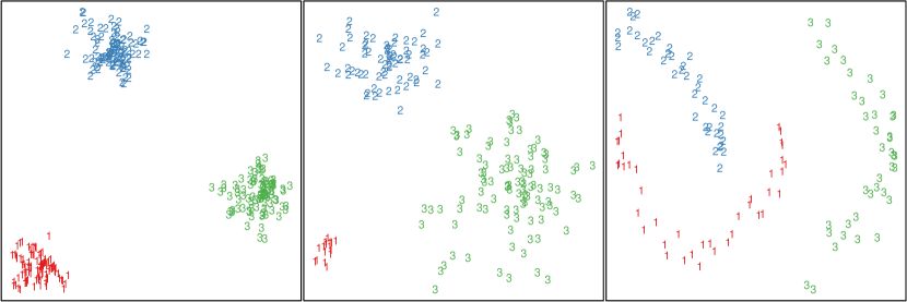
Figure 2: Illustration of clustering concepts including the true cluster membership indicators indicated by colour and using numbers for the data points: (a) compact clusters (on the left); (b) density-based clusters (in the middle); (c) connected clusters or clusters sharing a functional relationship (on the right).

The application of standard model-based clustering methods in general does not ensure that compact, high density or connected clusters or clusters with distinctly different functional relationships are obtained and heuristic methods might be easier to tune to address any of these notions. However, this also implies that the heuristic methods are more rigid in the solutions detected and might be more likely to come up with a specific clustering solution regardless of the inherent structure in the data. Thus solutions obtained using model-based clustering techniques which are agnostic of these cluster requirements can be assessed regarding these characteristics to verify if such a structure might inherently be present in the data. This also emphasises the need for specifying a suitable mixture model as well as applying appropriate post-processing methods to ensure that the outcome of model-based clustering is a useful clustering solution.

2 Specifying the model

For model-based clustering, finite as well as infinite mixture models have been used to fit a suitable distribution to the data and, in a subsequent step, to infer the cluster memberships from the fitted distributions and, potentially, also gain insights about typical characteristics of the cluster distributions. Fraley and Raftery (2002) point out that model-based clustering embeds the cluster problem in a probabilistic framework. The statistical framework allows to employ statistical inference methods for obtaining a suitable clustering of the data.

The starting point for model-based clustering is to define the distribution of a cluster and to decide how the cluster sizes are distributed. The definition of the cluster distribution can also be seen as the specification of the clustering kernel (see Frühwirth-Schnatter, 2011b). Depending on the available data and its characteristics, different kernels are suitable. In addition the purpose of the cluster analysis and characteristics of the intended cluster solution also guide the choice of the clustering kernel. The requirement that a cluster distribution needs to be specified makes model-based clustering in general more transparent with respect to the targeted clustering solutions, while in applications of heuristic methods the characteristics of the targeted clustering solutions often remain implicit.

Heuristic clustering is based on notions of similarity and dissimilarity between observations and groups of observations. Model-based methods also use a notion of similarity between observations. In the case of model-based methods observations in the same cluster share the characteristic that they are generated from the same cluster distribution. Observations are “similar” if they are generated by the same cluster distribution. The dissimilarity between observations in different clusters is influenced by the differences allowed for the cluster distributions.

If the same parametric distribution is assumed for each of the clusters, differences between cluster distributions are determined by the specific parameter values only. In the case of mixtures of multivariate Gaussian distributions for example often a centroid-based approach is pursued. The cluster means are assumed to differ and characterise the cluster distributions while the cluster covariance matrices rather represent nuisance parameters. The cluster covariance matrices might differ over clusters, but potentially could also be similar. If the covariance matrices are fixed to be identical over clusters, the dissimilarity between clusters is solely based on the cluster centroids. The conditional probabilities of cluster membership of an observation are then based on the Mahalanobis distance between the observation and the cluster centroid weighted by the cluster sizes.

2.1 Components corresponding to clusters

If mixture models are used for model-based clustering, the standard assumption is that each of the components in the mixture model corresponds to a cluster in the clustering solution. This implies that the component distribution specified in the mixture model is also the assumed cluster distribution.

For the specification of the mixture model it needs to be decided first if the clusters are expected to all follow a distribution from the same family of parametric distributions and that they differ only in the values of the parameter vectors or if different parametric distributions are assumed for the different clusters. The later might only be possible in cases where a clear notion of the latent groups to be detected is available. For instance, if the presence of two groups corresponding to healthy and ill persons is assumed and also some prior knowledge is available that the distributions of these two groups are structurally different. Otherwise – which is the usual case – the model specification is a priori the same for all of the components, i.e., the same (parametric) model is imposed and components differ only in the specific values of the parameters.

The choice of distribution for the components is governed by two aspects: (1) the data structure and (2) the suspected cluster distributions. In particular the data structure can easily be verified and has led to a standard set of mixture models to be considered for certain kinds of data, e.g., multivariate continuous data, multivariate categorical data, multivariate mixed data or longitudinal data.

Multivariate continuous data.

For model-based clustering of multivariate continuous data of dimension $d$ the standard model is the finite mixture model of multivariate Gaussian distributions given by

$$y_{i} \sim\sum_{g=1}^{G}\eta_{g}\phi(y_{i}|\mu_{g},\Sigma_{g}).$$

The advantages of Gaussian mixture modelling are that estimation methods are well established and that the component distributions are thoroughly understood and thus interpretation of results is facilitated. Drawbacks are that the likelihood is unbounded for arbitrary covariance matrices $\Sigma_{g}$ because of singular solutions leading to spurious results. Results are also strongly susceptible to extreme observations because of the light tails of the Gaussian distribution. When clustering data, it is often essential that the means of the cluster distributions are different and can be used as centroids to represent the clusters. However, this is not necessarily achieved when using this standard model class because there are no constraints – neither implicitly nor explicitly – imposed which would ensure that the fitted mixture model has these characteristics.

If a centroid-based approach to clustering is pursued, the covariance matrices of the components in the mixture model are seen as nuisance parameters which need to be suitably parameterised to allow for identification of the clusters. In particular for high-dimensional data the specification of the covariance matrices is crucial because they add a substantial number of additional parameters to the model as the number of parameters of a single, unrestricted covariance matrix is $d(d+1)/2$ for data of dimension $d$.

To achieve a parsimonious parameterisation, different variants to impose restrictions on the covariance matrices based on the spectral decomposition of the covariance matrix into shape, volume and orientation have been proposed in Banfield and Raftery (1993) and are also discussed in Celeux and Govaert (1995) and Fraley and Raftery (2002). The decomposition of the covariance matrix of the $g$-th component is given by

$$\Sigma_{g} =\lambda_{g}D_{g}A_{g}D_{g}^{\top},$$

where the positive scalar $\lambda_{g}$ corresponds to the volume, the $d\times d$ matrix $D_{g}$ to the orientation and the $d$-dimensional diagonal matrix $A_{g}$ to the shape. More parsimonious parameterisations can be achieved by restricting the components of the decomposition to be equal over components and by imposing certain values, e.g., assuming $D_{g}$ to be the identity matrix.

An alternative approach for a parsimonious parameterisation of the covariance matrices is to assume a latent structure leading for example to factor analysers as models for the covariance matrices (McLachlan and Peel, 2000b) or the unified latent Gaussian model approach which encompasses factor analysers and probabilistic principal component analysers as special cases (McNicholas and Murphy, 2008).

The use of mixtures of Gaussian distributions for clustering data imposes a prototypical shape on the clusters which implies symmetric and light tailed distributions. However, often in applications clusters are assumed to have different shapes, e.g., data clusters could exhibit skewed shapes and contain outlying observations. In order to account for skewness the extension to multivariate skew-normal distributions (Azzalini and Dalla Valle, 1996) has been considered and for a more robust method the $t$-distribution is used for the components. For an application in the mixture context see Frühwirth-Schnatter and Pyne (2010), Lee and McLachlan (2013) and Lee and McLachlan (2014). Further approaches considered for example the use of shifted asymmetric Laplace distributions (Franczak et al., 2014) or multivariate normal inverse Gaussian distributions (O’Hagan et al., 2016).

Multivariate categorical data.

In the context of multivariate binary data the latent class model has been developed as a useful tool for clustering (Goodman, 1974). This model can also be easily extended to the case of categorical data. Latent class models aim at explaining the dependency structure present in the multivariate data by introducing a discrete latent variable, i.e., the cluster membership, such that conditional on the latent variable the observations in the different dimensions are independent. This assumption is also referred to as conditional local independence. The latent class model for multivariate binary data is given by

$$y_{i}\sim\sum_{g=1}^{G}\eta_{g}\left[\prod_{j=1}^{d}f_{\mathcal{B}er}(y_{ij}|\pi^{j}_{g})\right],$$

where $f_{\mathcal{B}er}(\cdot|\pi)$ is the density of the Bernoulli distribution with the success parameter $\pi$ and $\pi^{j}_{g}$ is the success probability for the $j$-th variable and the $g$-th component.

Multivariate mixed data.

The conditional local independence assumption can also be used for modelling mixed data. For groups of variables where a joint distribution allowing for dependencies might be hard to specify for the components, a product of the univariate distributions is used (Hunt and Jorgensen, 1999). Thus as long as a suitable parametric distribution is available in the univariate case a mixture model can be specified and fitted.

Alternatively an approach has been proposed which uses the following model for the components: the data in each cluster is assumed to be generated based on a latent variable which follows a multivariate Gaussian distribution where an arbitrary covariance matrix can be used. The latent variable is then mapped to the observed measurement scale, e.g., a binary or ordinal variable (Cai et al., 2011; Browne and McNicholas, 2012; Gollini and Murphy, 2014).

Multivariate data with special structures.

Special structures in multivariate data sets occur because of the variables having different roles or because of specific constraints restricting the values of the variables which can jointly be observed. If one variable represents a dependent variable and the others explanatory variables this leads to a regression setting. Multivariate data occurring only on a restricted support than the one induced by taking the product of the support of each of the univariate variables require to take this into account in model specification. Graph or network data also have a specific multivariate data structure.

In a regression setting one variable is identified as the dependent variable $y$ and all other variables act as potential independent variables $x$. The mixture model is then given by

$$y_{i}|x_{i} \sim\sum_{g=1}^{G}\eta_{g}f(y_{i}|x_{i},\theta_{g}),$$

where $f(\cdot)$ represents a regression model and $\theta_{g}$ contains the regression parameters of component $g$. Clearly any regression model could be used for the components and identified with a cluster. The selection of the regression models for the components needs to ensure that any other inherent structure in the multivariate data set is captured. For example, repeated observations might be taken into account by including random effects.

Identifiability might be an issue in the context of mixtures of regressions (Follmann and Lambert, 1991; Hennig, 2000; Grün and Leisch, 2008). If the mixture model specified is not identifiable this implies that neither the parameter estimates used to characterise the clusters nor the partitions derived can be uniquely determined thus rendering the interpretation of results futile. If the non-identifiability leads to two or more isolated clearly differing solutions which are observationally equivalent, the data does not allow to distinguish between them. In this case domain knowledge might help in deciding which of these solutions represents a useful clustering and allow to exclude the alternative solutions.

Specific models might be useful if the multivariate data has a restricted support, for instance, when the observations or their squared values sum to one, in which case the multivariate data points have the unit simplex or the unit hypersphere as support. Clustering data on the unit hypersphere is sometimes also seen as clustering data only with respect to the directions implied, while neglecting the length information of the data points. Using a component distribution which has as support the unit hypersphere leads for example to mixtures of von Mises-Fisher distributions (Banerjee et al., 2005). This model has also been shown to represent the corresponding probabilistic model for spherical clustering where cosine similarity is used as similarity measure in $k$-centroid clustering, similar to how Gaussian mixtures are a probabilistic model for $k$-means clustering.

Analysing the topology of systems of interacting components is based on network data where the components correspond to nodes and their interactions to edges. This graph or network data represents a specific data structure and is often stored using an adjacency matrix. If the data contains $n$ nodes, the adjacency matrix is of dimension $n\times n$ and the entries reflect if there are edges between nodes together with the edge weights. In the simple case of a symmetric, unweighted graph, the adjacency matrix is a symmetric binary matrix. Clustering methods applied to network data aim at finding community structures or at grouping nodes together which are similar in their interactions (Handcock et al., 2007; Newman and Leicht, 2007).

2.2 Combining components to clusters

While mixture models as considered in Section 2.1 often are able to capture the data distribution, the assumption that there is a one-to-one relationship between components and clusters might be violated. Some components might be too similar to form separate clusters and should rather be merged.

In this situation, a mixture of mixtures model can be useful where groups of components are combined to form a single cluster. The inference on clusters can be either performed simultaneously with model fitting or as a subsequent step, after having fitted a suitable model for approximating the data distribution. In the following, several strategies are discussed for multivariate continuous data and some of these strategies might also be employed for other types of multivariate data.

Finite mixtures of Gaussian distributions are not only a suitable model for model-based clustering, but can also be applied for semi-parametric approximation of general distribution functions. A hierarchical mixture of mixtures of Gaussian distributions model can thus be used in a situation where a single Gaussian distribution is not flexible enough to capture the cluster distribution. In this hierarchical model the components on the upper level of the mixture correspond to clusters, while those on the lower level are only used for semi-parametric estimation of the cluster distribution.

In its hierarchical structure the model is given by

$$p(y_{i}|\theta) =\sum_{g=1}^{G}\eta_{g}f_{g}(y_{i}|\theta_{g}),$$

$$f_{g}(y_{i}|\theta_{g}) =\sum_{h=1}^{H_{g}}w_{gh}\phi(y_{i}|\mu_{gh},\Sigma_{gh}).$$

While such a model is appealing as it involves only Gaussian distributions and thus is easy to understand and implement, identifiability of the model is an issue because the likelihood is invariant to assignment of components on the lower level to clusters on the upper level. In fact the density implied by this hierarchical representation is equivalent to

$$p(y_{i}|\theta) =\sum_{g=1}^{G}\sum_{h=1}^{H_{g}}\eta_{g}w_{gh}\phi(y_{i}|\mu_{gh},\Sigma_{gh}).$$ (1)

This is to say that the hierarchical mixture of Gaussian mixtures model is equivalent to a mixture of Gaussian distributions with $\tilde{G}=\sum_{g=1}^{G}{H_{g}}$ components with weights $\eta_{gh}=\eta_{g}w_{gh}$ and component-specific parameter vectors $\mu_{gh}$ and $\Sigma_{gh}$. Clearly the components in Equation (1) can be arbitrarily regrouped to form clusters without changing the overall density.

To achieve identifiability in a hierarchical mixture of mixtures model several approaches were proposed. They differ in that either identification is already aimed for during model fitting or that first a suitable semi-parametric approximation of the data distribution is obtained using mixtures of Gaussian distributions and then a second step is used for forming clusters by combining components.

Direct inference for the mixture of mixtures approach.

In order to directly fit this kind of model strong identifiability constraints were imposed in a maximum likelihood framework. Bartolucci (2005) considers only the case of univariate data and specifies a mixture of Gaussian mixtures model where the mixtures on the lower level are restricted to be unimodal and to be the same for all clusters except for a mean shift. A similar restriction to have the same mixture distribution on the lower level except for a mean shift was considered in Di Zio et al. (2007) for multivariate data.

Within a Bayesian framework the identifiability issue present due to the invariance of the likelihood can be resolved by specifying informative priors which allow to automatically distinguish between components from the same and different clusters. Malsiner-Walli et al. (2017) consider this approach for finite mixtures, whereas Yerebakan et al. (2014) use an infinite mixture approach. Malsiner-Walli et al. (2017) proposed a prior structure which reflects the prior assumptions on the separateness of the clusters and the compactness of their shapes and which can be suitably adapted for different kinds of applications. Thus the clustering notions, i.e., the cluster solutions aimed for, are explicitly included in the mixture model using informative priors in a Bayesian setting. Their prior also implies that the mixture on the lower level used for approximating the cluster distributions is allowed to contain components with different covariance matrices, but where the component means are pulled towards a common mean corresponding to the centre of the cluster. The prior structure employed by Yerebakan et al. (2014) is more rigid. In their approach the covariance matrices on the lower level are assumed to be the same within a cluster and also that the mean parameters on the lower level scatter according to a scaled version of the same covariance matrix.

Two-step procedures.

In the first step mixtures of multivariate Gaussians are fitted as semi-parametric approximations of the data distribution. The use of multivariate Gaussian mixtures for the semi-parametric approximation raises another issue. Often different Gaussian mixture models allow to similarly well approximate the data distribution because the approximation might either use only few components with complex component distributions or many components with simple component distributions. In case of Gaussian mixture models the complexity of the component distribution is primarily governed by the structure of the covariance matrix.

Subsequently a merging approach is employed in order to form meaningful clusters given the Gaussian components. Different criteria were proposed for deciding on merging in a stepwise procedure such as closeness of the means (Li, 2005), the modality of the resulting clusters (Chan et al., 2008; Hennig, 2010), the entropy of the resulting partition (Baudry et al., 2010), the collocation of the observations (Molitor et al., 2010), the degree of overlap measured by misclassification probabilities (Melnykov, 2016), and the the use of clustering cores (Scrucca, 2016).

This second step corresponds to another cluster analysis being performed where the input are not the data points, but the estimated mixture components. The mixture is assumed to be too fine-grained to represent a good cluster solution and groups of components need to be formed to obtain the clusters. Note that in particular those approaches which only take the conditional probabilities of component memberships or collocations of observations into account can directly be used for any kind of mixture models to merge components to clusters regardless of the distributions used for the components of the mixture.

2.3 Selecting the clustering base

The variables included as clustering base are in general assumed to all equally contribute to the clustering solution. Each of the variables is assumed to be in line with and reflect the cluster structure. In general the variables used for cluster analysis should be carefully selected because choosing a different set of variables might change the meaning of the resulting cluster solution (Hennig, 2015). Even efforts are made to select a suitable clustering base based on theoretic considerations driven by domain knowledge, the selected variables might not all be equally useful to cluster the data or contribute equally to a selected clustering solution. In fact some of the variables included in the cluster base might turn out to either contain no cluster structure or be irrelevant for the obtained clustering solution. The inclusion of irrelevant variables has several drawbacks. In particular their inclusion complicates model selection due to overfitting and makes the interpretation of the cluster solution a harder task than necessary. In the worst case some variables might even perturb the cluster structure detected. Such variables are referred to as masking variables and if included deteriorate the cluster solution.

Alternatively the aim could be to reduce the clustering base in order to eliminate redundant variables. This approach assumes that the clustering information contained in a subset of the variables is sufficient to characterise the cluster solution obtained using all variables. This task thus requires to identify the minimal set of variables necessary to identify the cluster solution. Using only the smaller set then might get rid of collinearity problems, reduces the number of variables which need to be collected for future analyses and facilitates the interpretation by providing a core set of essential variables.

A range of variable selection methods for clustering have been proposed which can be used in the heuristic and / or the model-based context and which can be either applied prior to, during or after the cluster analysis to identify a suitable subset of variables (Gnanadesikan et al., 1995; Steinley and Brusco, 2008b).

Prior filtering.

Prior filtering investigates the distribution of single variables and assesses how well suited they might be to reveal cluster structure in the data. Variables with a very homogeneous distribution do clearly not allow to extract clusters from the data. These variables can be excluded from the clustering base before performing the cluster analysis. Clearly for very high-dimensional data prior filtering is appealing because this might allow to substantially reduce the dimensionality of the clustering problem.

In particular for continuous variables, indices to assess the clusterability of a variable were developed. These clusterability indices aim to determine whether a variable allows to meaningfully cluster the observations or if the observations exhibit a tendency to form into clusters based on a specific variable. Steinley and Brusco (2008a), for instance, propose to use a variance-to-range ratio for initial screening of each variable and to exclude variables where these ratios are small.

Variable selection.

Deciding on a suitable variable set during finite mixture model estimation often is complicated by the fact that the suitability of a variable set depends on the number of clusters and the specific component model used, e.g., the specification of the covariance matrices in Gaussian mixture modelling. Thus the decision on the variable set needs to be made simultaneously while deciding on a suitable number of clusters and component model.

Heuristic methods for exploring the model space with respect to different number of clusters and variable sets have been proposed in Raftery and Dean (2006), Maugis et al. (2009) and Dean and Raftery (2010) for Gaussian mixture models and latent class analysis using maximum likelihood estimation and the Bayesian information criterion (BIC) for model comparison.

Alternatively within a Bayesian framework Tadesse et al. (2005) propose to use reversible jump Markov chain Monte Carlo (MCMC) methods in Gaussian mixture modelling to move between mixture models with different numbers of components while variable selection is accomplished by stochastic search through the model space. In the context of infinite mixtures Kim et al. (2006) combine stochastic search for cluster-relevant variables with a Dirichlet process prior on the mixture weights to estimate the number of components. White et al. (2016) suggest to use collapsed Gibbs sampling in the context of latent class analysis to perform inference on the number of clusters as well as the usefulness of the variables.

Shrinkage methods.

A different approach to address the variable selection problem is to use shrinkage or penalisation methods. In a frequentist setting these methods correspond to maximising a penalised likelihood while in a Bayesian setting suitable priors are used to induce shrinkage. This approach aims to induce solutions which favour a homogeneous distribution over some variable or parameter in case the evidence for heterogeneity is insufficient. This allows to prevent overestimating heterogeneity and provides insights into which variables or parameters are relevant for the cluster solution.

The shrinkage approaches pursued build on work in regression analysis for variable selection. In this context for example the lasso (least absolute shrinkage and selection operator; Tibshirani 1996) was proposed to perform variable selection. For the lasso penalty the penalised likelihood estimate has exact zeros for some of the regression coefficients instead of small values. Similar results are obtained for the maximum a-posteriori estimate if the lasso is used as prior for the regression coefficients. In the mixture context the lasso penalty or prior is imposed on the parameter representing the difference between the cluster value and the overall value of the parameter thus inducing solutions where these differences are shrunken towards zero and the overall value of the parameter is the same over all clusters.

In Gaussian mixture models shrinkage approaches have been proposed which only impose the penalty or shrinkage prior on the cluster means. This specification of the shrinkage reflects the assumption that the component means characterise the clusters and thus are different for variables relevant for clustering. This approach was used in Pan and Shen (2007) using penalised maximum likelihood estimation. Using a fully Bayesian approach Malsiner-Walli et al. (2016) employed the normal-gamma prior for the differences in the component means using finite mixtures and Yau and Holmes (2011) imposed a double exponential prior on the differences in the component means while fitting infinite mixtures.

Post-hoc selection.

This approach aims at arriving at a cluster solution for a subset of variables which is similar to the cluster solution obtained using all variables. This procedure is based on the assumption that the clustering base does not contain any masking variables, but the best cluster solution is obtained using all variables. However, some of the variables might be redundant because they either contain no or the same information on the cluster structure than other variables in the segmentation base. In the post-hoc selection step the aim is to identify these redundant variables and omit them. After omitting these variables the cluster problem has been recasted a a lower dimensional problem and results are easier to interpret. Fraiman et al. (2008) for example propose two procedures to identify such variables assuming that a “satisfactory” grouping is given.

2.4 Selecting the number of clusters

Selecting the number of clusters is quite a controversial topic. For finite mixtures, a suitable number of components can be selected using different criteria. Information criteria such as the Akaike information criterion (AIC) or Bayesian information criterion (BIC) have been used in a model-based clustering context where it has been shown for the BIC that the number of components are consistently selected under certain conditions, in particular ensuring that the component densities remain bounded (Keribin, 2000).

If the model is fitted as part of the merging approach, there has been less controversy around methods to select a suitable model. In this case only a suitable semi-parametric approximation is required and the determination of the number of clusters is made in the subsequent step.

In the case where components are assumed to correspond to clusters, the situation is more complicated. Mixture models cannot only be used to obtain a clustering, but also for semi-parametric density approximation. Information criteria developed for general model assessment usually aim at identifying a solution which reflects the data-generating process well and thus rather select a model which represents a well semi-parametric approximation of the data distribution. The information criteria are ignorant of the clustering purpose the model is finally used for. In case where the component distribution does not exactly match the cluster distribution, the number of clusters tends to be overestimated using these criteria. This problem becomes more severe the more data is available. The larger the data set the better the cluster distributions can be estimated and deviations from the imposed parametric distribution are more severely penalised.

In order to improve the model selection performance when using mixture models of parametric distributions for model-based clustering, an alternative criterion was proposed. This criterion does not only measure the suitability of a model based on the goodness-of-fit for the data distribution, as indicated by the log-likelihood, but also how well observations can be assigned to clusters. The later is equivalent to having well separated cluster distributions where the conditional probabilities of component membership unambiguously allow to assign the observations to one of the components. Thus the entropy of the conditional probabilities of component membership is also taken into account leading to the integrated completed likelihood information criterion (ICL; Biernacki et al., 2000), i.e.,

$$\text{ICL}(G) =\sum_{i=1}^{n}\log f(y_{i},\hat{z}_{i}|G,\hat{\theta})-\frac{\upsilon_{G}}{2}\log n,$$

where $\hat{z}_{i}$ is the estimated cluster membership for observation $i$, $\hat{\theta}$ the estimated mixture parameters and $\upsilon_{G}$ the number of estimated parameters. In contrast to AIC or BIC, ICL aims at identifying well separated clusters. This avoids overestimating the number of clusters by taking into account that the estimated model is used to assign observations to clusters and to obtain a suitable partition of the observations.

3 Post-processing the fitted model

3.1 Identifying the model

Mixture models suffer from generic non-identifiability issues due to label switching (Redner and Walker, 1984), i.e., the mixture distribution is the same regardless of which label is assigned to which cluster. Only inference on label invariant quantities can be easily accomplished while inference on quantities which depend on a unique labelling require an identified mixture model.

If only point estimates of mixture models are used, such as maximum likelihood estimates in a frequentist framework or maximum a-posteriori estimates in a Bayesian setting, a unique solution is easily obtained by imposing an ordering constraint. If uncertainty estimates based on bootstrap techniques in frequentist estimation and MCMC samples in Bayesian estimation with symmetric priors are to be derived, the situation is more complicated and different methods for obtaining an identified model have been proposed including (a) imposing an ordering constraint (Frühwirth-Schnatter, 2001), (b) applying label-invariant loss functions in cluster and relabelling algorithms (Stephens, 2000), (c) fixing the component membership of some observations (Chung et al., 2004), (d) relabelling with respect to the point estimate, e.g., the maximum a-posteriori estimate (Marin et al., 2005), (e) clustering in the point process representation (Frühwirth-Schnatter, 2006, 2011a), (f) probabilistic approaches taking the uncertainty of the relabelling into account (Sperrin et al., 2010). For an overview see also Jasra et al. (2005) and Papastamoulis (2016).

3.2 Determining a partition

Binder (1978) considered Bayesian cluster analysis as the task to determine a suitable partition given a data set and assuming an underlying mixture model. Thus more work has been done in the Bayesian context to obtain a suitable partition based on $P(\bm{z}|\bm{y})$. In the frequentist setting a partition is in general determined using an identified model to classify observations separately and obtain a partition.

In the Bayesian context Binder (1978) proposed to obtain the optimal partition by minimising the expected loss given $P(\bm{z}|\bm{y})$ and suggested several different loss functions. This approach corresponds to minimising

$$\mbox{E}(\ell(\hat{\bm{z}},\bm{z})|\bm{y})$$

with respect to $\hat{\bm{z}}$ given the loss $\ell(\cdot,\cdot)$ between two classifications of the data. One possible loss function is to use the 0/1 loss, where

$$\ell(\hat{\bm{z}},\bm{z}) =\left\{\begin{array}[]{ll}0&\text{if }\hat{\bm{z}}=\bm{z},\\ 1&\text{if }\hat{\bm{z}}\neq\bm{z}.\\ \end{array}\right.$$

or a label-invariant version thereof. Using the 0/1 loss function results in the maximum a-posteriori estimate, i.e., leads to selecting the mode of $P(\bm{z}|\bm{y})$. The drawback of the 0/1 loss is that as long as two classifications are not the same they are assessed as equally different by assigning a loss of one. This has lead to a number of alternative loss functions being suggested. Depending on the loss function used in general either an identified model or the posterior distribution of collocation is required to determine the loss minimising classification. For more details see also Frühwirth-Schnatter (2006, Section 7.1.7).

Based on an identified model.

Given an identified model the cluster memberships can be inferred from the latent allocation variables $z_{i}$ and conditional on the parameters $\theta$ of the mixture model. In this case the latent allocation variables are independent and group memberships can be inferred separately for each observation based on the conditional distributions of cluster memberships $\mathbf{z}=(z_{1},\ldots,z_{n})$ given the data $\mathbf{y}=(y_{1},\ldots,y_{n})$,

$$\Prob(z_{1}=g_{1},\ldots,z_{n}=g_{n}|\mathbf{y},\theta)\propto\prod_{i=1}^{n}\eta_{g_{i}}f_{g_{i}}(y_{i}|\theta_{g_{i}}),$$

where $g_{i}$ is the cluster observation $y_{i}$ is assigned to. To determine a clustering different estimates can be used based on the conditional probabilities of cluster memberships, e.g., observations can be assigned to the cluster they are most likely from or assigned by drawing from the conditional probabilities.

Assigning the observations to the cluster they are most likely from results in the classification which is also obtained when minimising the misclassification rate as loss function. This classification is obtained by setting

$$\hat{z}_{i} ={\arg\,\max}_{g}\Prob(z_{i}=g|y_{i},\theta)$$

for each observation $i$.

Based on the collocation matrix.

Partitions have the advantage that they are label-invariant quantities. This implies that procedures for determining a final partition can be used which do not require an identified model, but only use the estimated collocation of observations as input. This also implies that the only output required from model fitting is the information on the partitions, i.e., collapsed sampling schemes can be used in an MCMC context.

The collocation matrix is a $n\times n$ matrix of values between 0 and 1 with 1s in the diagonal where the $(i,j)$ entry represents the probability that observations $i$ and $j$ are assigned to the same component of the fitted mixture model, i.e., $P(z_{i}=z_{j}|\bm{y})$. Several approaches for deriving a suitable partition from such a collocation matrix have been proposed in a Bayesian setting where draws from the posterior distribution of partitions are available. These suggestions include (a) minimising a pairwise coincidence loss function (Binder, 1978; Lau and Green, 2007), (b) reformulating $P(z_{i}=z_{j}|\bm{y})$ as a dissimilarity matrix and using partitioning around medoids (PAM; Kaufman and Rousseeuw, 1990), a standard partitioning clustering technique (Molitor et al., 2010), (c) determining a partition which minimises the squared distance as loss function (Fritsch and Ickstadt, 2009), and (d) minimising the variation of information as loss function (Wade and Gharhamani, in press). Of particular note is that the partition minimising the posterior expected loss can in general not be obtained directly, but iterative optimisation methods need to be employed. Due to the size of the partition space this is a computational demanding task.

3.3 Characterising clusters

Cluster analysis aims at determining groups in the data. The results of a cluster analysis, however, in general not only consist of a partition of the data, but also a characterisation of the groups. The clustering together with the characterisation of the clusters allows to summarise a multivariate data set and to give insights into its structure. The characterisation of the clusters allows to profile them and provides insights into the latent groups or types identified. This can be used to describe the groups or even assign them meaningful names.

In heuristic cluster analysis often a prototype for each group or cluster is determined. In model-based clustering the cluster distributions allow to characterise the clusters. If parametric distributions are used for the clusters, often focus is given to reporting and comparing the parameter estimates together with their associated uncertainty.

Comparing the differences between prototypes in heuristic clustering is not straightforward because the clustering algorithm aimed at maximising these differences. Model-based methods thus allow to assess differences between clusters using a sound statistical framework. This facilitates to identify the variables which contribute most to the clustering, and to assess if the resulting clustering is useful. The cluster distributions can either be determined based on an identified mixture model or conditional on the partition or clustering obtained for the data.

3.4 Validating clusters

General validation techniques have been developed for cluster analysis which can be used regardless of the clustering method used. These validation methods are distinguished into internal, external and stability-based methods. Furthermore the assessment can be on the level of the global cluster solution or specific to a single cluster. A general overview on cluster validation methods is for example given in Halkidi et al. (2001), while Brock et al. (2008) provide an overview on internal and stability-based measures as well as biological ones in the context of bioinformatic applications.

Internal measures.

The use of internal measures is appealing because they only require data which is already available. However, they rely on a notion of distance between observations. This notion is readily available when heuristic clustering methods are applied. For the application of model-based clustering methods no distance or dissimilarity measure between observations needs to be specified. So this needs to be additionally done in order to be able to calculate the internal measures.

Most of the internal measures include information on within-cluster scattering (i.e., compactness) and between-cluster separation. Examples for these measures are silhouette width (Rousseeuw, 1987), the Dunn index (Dunn, 1974) or the Davies-Bouldin index (Davies and Bouldin, 1979). However, these measures are in general only useful for convex shaped clusters and fail to provide suitable insights into the quality of a cluster solution in cases of arbitrarily shaped non-convex clusters and if noisy observations are present. It is also obvious that if the internal criterion coincides with the criterion minimised in the algorithm used for heuristic clustering the solution obtained with this method should perform well. This thus seems to be an unfair comparison. Nevertheless it might still be useful to compare different cluster results on this basis. This comparison provides insights into how much worse alternative solutions are which are derived using a different cluster criterion. Such an investigation might also not only provide insights into the cluster solutions obtained, but also what kind of cluster structure might naturally be contained in the data.

Also internal measures specifically developed for the mixture model context have been proposed. Celeux and Soromenho (1996) suggest to assess the suitability of a fitted mixture model to be used for clustering based on the entropy of the conditional probabilities of cluster memberships. Because the final partition of the data is derived from these conditional probabilities of cluster memberships, a mixture model is more suitable for clustering if observations can be unambiguously assigned to clusters. This measure also captures the loss of information incurred by using only the estimated partition as result and neglecting the uncertainty of cluster assignment.

External measures.

External measures relate the partition derived to some external structure, i.e., partition, imposed on the data. For instance, an additional categorical variable is available which induces a partition of the data, but has not been used in the cluster analysis. Such a comparison assumes implicitly that the aim of the cluster analysis was to arrive at a partition of the data which is close to this partition. In general using cluster analysis to extract a partition which corresponds to a partition induced by an observed categorical variable is questionable. If the target variable is observed it would seem more natural to use a classification or supervised learning approach.

Standard methods for assessing classification accuracy, e.g., the misclassification rate, can be employed to compare the class labels to the cluster labels. However, this approach requires that a mapping from cluster labels to class labels needs to be determined, which might eventually not be straightforward in case where the number of clusters and classes are different. One approach might be to choose the mapping which maximises the classification accuracy criterion employed. As an alternative, label-invariant measures can be employed which determine the similarity between two partitions regardless of any labels assigned to each of the groups contained in the partitions. This is achieved by determining the numbers of pairs of observations which are in the same group for both partitions, in different groups for both partitions and in different groups in one partition and in the same group for the other. Based on these numbers of pairs the Rand index (Rand, 1971) or adjusted Rand index (Hubert and Arabie, 1985), the Jaccard coefficient (Jaccard, 1912), the Fowlkes and Mallows index (Fowlkes and Mallows, 1983) among others can be derived and used as validation measures. A further criterion used is purity (Zhong and Ghosh, 2003) which assesses to which extent a cluster only contains observations from the same class, i.e., this criterion does not penalise splitting classes into several clusters, but deteriorates if classes are merged into the same cluster.

Stability measures.

External measures compare two partitions. These measures thus can also be used to assess the stability of cluster solutions (see for example Hennig, 2007). The extent to which a cluster solution depends on a specific data set and how much it varies if a new data set is used can be assessed based on bootstrapping. Pairs of bootstrap samples are drawn from the data and clustered. These two cluster solutions induce each a partition in the original data set. The similarity between these partitions is determined using an external measure and can be used to assess stability. Alternatively it might also be of interest to assess stability of clustering solutions if different cluster algorithms are employed.

Dolnicar and Leisch (2010) point out that these stability assessments allow to infer if cluster solutions can at least be constructed in a stable way in the case when natural clusters, i.e., density clusters, are not contained in the data. They propose to use stability as a criterion to select a suitable clustering solution in case no natural clusters are contained in the data set.

3.5 Visualising cluster solutions

Suitable visualisation methods allow to assess the cluster quality, illustrate the cluster shapes and gain an insight into the cluster distributions. Visualisation is of particular importance in the clustering context as clustering is an exploratory data analysis tool. Assessing the quality of a cluster solution based on visualisations is also often necessary because of the difficulty to formally define the clustering problem in a way which ensures that the obtained solutions have the desired characteristics. Furthermore, input from domain experts to validate and optimise a cluster solution might be easier to obtain if they are able to assess a suggested solution using suitable visualisations.

Assessing cluster quality.

Given different cluster validation indices it might be easier to compare them and select a suitable solution in dependence of their values using visualisation methods. E.g., if a clear cluster structure is suspected in the data an elbow or optimal value of the criterion might be visually discernible and used for model selection. In the merging components to clusters context Baudry et al. (2010) suggest to plot the entropy values versus the number of clusters and select the solution where there is a break point in a piecewise linear fit.

An additional visualisation technique based on an internal cluster validation index is the silhouette plot (Rousseeuw, 1987). The silhouette plot illustrates the quality of the cluster solution based on the silhouette values grouped by cluster. As an alternative Leisch (2010) proposed the shadow plot which has the same structure but uses the shadow value instead of the silhouette value. The shadow value has the advantage that it is computationally less demanding to determine than the silhouette value. The drawback is that this index relies more on the cluster centroid being a good representative.

Illustrating cluster shapes and separation.

Cluster shapes and separateness can be illustrated using scatter plots of the data points, at least for continuous data. However, in the case of high-dimensional data this might not be a feasible approach and lower dimensional representations of the data might be more useful. The lower dimensional representations could either be based on general techniques for dimension reduction such as principle component analysis (PCA) or specific techniques for cluster analysis. In the context of Gaussian mixture modelling Scrucca (2010) proposes to determine the subspace which captures most of the cluster structure contained in the data. Alternatively also cluster-specific projections were proposed which for a given cluster maximises its distance to the other clusters (Hennig, 2004).

Characterising cluster prototypes.

Profile plots of the prototypes can help to quickly identify in which variables clusters differ and how they can be characterised (Dolnicar and Leisch, 2014). Profile plots use the information on the prototypes and visualise them. In the model-based context this information consist of characterisations of the cluster distributions, e.g., in case of parametric distributions their parameters. Profile plots are based on conditional plots and separately visualise each of the cluster results, but allow for easy comparison. These plots can also be enhanced to include uncertainty information.

In the context of shrinkage priors imposed on the cluster means Yau and Holmes (2011) and Malsiner-Walli et al. (2016) propose to visualise the posterior distribution of the shrinkage factors for each of the variables using boxplots. Such a visualisation indicates the variables for which the clusters differ and thus can be used to characterise the clusters.

Visualising the example data sets.

The three data sets introduced in Section 1.3 and shown in Figures 1 and 2 are used to create silhouette plots and to visualise in a silhouette-type plot the cluster uncertainty inherent in fitted suitable mixture models.

The silhouette value for an observation $i$ is given by

$$s(i) =\frac{b(i)-a(i)}{\max\{a(i),b(i)\}},$$

where

$$a(i) =\frac{1}{n_{z_{i}}}\sum_{j\in{\cal C}_{z_{i}}}\|y_{i}-y_{j}\|,$$

$$b(i) =\min_{g\in\{1,\ldots,G\}\setminus z_{i}}\frac{1}{n_{g}}\sum_{j\in{\cal C}_{g}}\|y_{i}-y_{j}\|,$$

i.e., $a(i)$ is the average Euclidean distance of observation $i$ to all observations $j$ assigned to the same cluster and $b(i)$ is the minimum average Euclidean distance of observation $i$ to observations $j$ which are assigned to a different cluster. This definition ensures that $s(i)$ takes values in $[-1,1]$, where values close to one indicate “better” clustering solutions.

Rousseeuw (1987) suggests to visualise the silhouette values by grouping them by cluster and sorting them in decreasing order within cluster. The width of the values for each cluster indicates the size of the cluster and the distribution of silhouette values within cluster indicates how well separated that cluster is from the other clusters in Euclidean space. The average silhouette value within a cluster serves as an indicator how compact and well separated this cluster is. The overall cluster solution can be assessed using the total average of silhouette values.

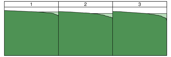
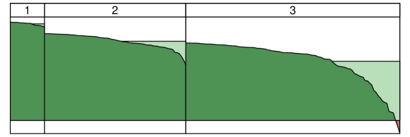
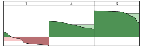
Figure 3: Silhouette plots based on the Euclidean distance and the true clustering for the three example data sets shown in Figure 1: (a) compact clusters (on the top); (b) density-based clusters (in the middle); (c) connected clusters or clusters sharing a functional relationship (on the bottom).

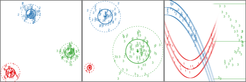
Figure 4: Plots of the example data sets together with the fitted mixture models: (a) a mixture of three Gaussian distributions with identical spherical covariance matrices (on the left); (b) a mixture of three Gaussian distributions with different spherical covariance matrices (in the middle); (c) a mixture of linear regression models with concomitant variables (on the right).

Figure 3 shows the silhouette values using Euclidean distance and the true clustering solution for the three artificial data sets. The plot on the top gives the silhouette plot in the case compact clusters are present. The result indicates that these clusters are well separated in Euclidean space and the plot also reflects that the clusters are equally sized. For the case of density-based clusters the silhouette plot indicates that the clusters are of different size and the different levels of compactness of the clusters impact the silhouette values within clusters (middle plot). For the case of connected clusters which might be modelled using some functional relationship the silhouette plot at the bottom indicates that centroid-based partitioning methods using the Euclidean distance might not be able to detect the true solution because most observations in the first cluster, i.e., the $U$-shaped cluster in Figures 1 and 2 on the right, are in Euclidean space closer on average to observations from a different cluster than their own.

If model-based clustering methods are used to fit the different data sets one can use: for data set (a) a mixture of Gaussian distributions with identical spherical covariance matrices, for data set (b) a mixture of Gaussian distributions with spherical covariance matrices differing in volume and for data set (c) a mixture of linear regression models with a horizontal line for the first cluster and polynomial regressions of degree two for the other two clusters in combination with a concomitant variable model (see also Section 4.2) based on the variable on the $x$-axis, i.e., the cluster sizes dependent on variable $x$ in the form of a multinomial logit model. The models obtained when fitted using the EM algorithm initialised in the true solution are shown in Figure 4. For the first two examples the cluster means are indicated together with the 50% and 95% prediction ellipsoids (neglecting the uncertainty with which the parameters are estimated) for the fitted components given by circles using full and dashed lines respectively. For the third example the fitted regression lines for each of the components are shown together with 95% pointwise prediction bands (neglecting the uncertainty with which the parameters are estimated) and using an alpha-shading (i.e., a transparency value) corresponding to the component size derived from the concomitant variable model. The points are numbered according to their component assignments based on the maximum conditional probabilities of cluster memberships obtained from the fitted mixture models.

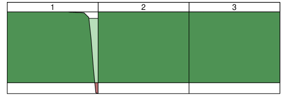
Figure 5: Plots of the conditional probabilities of cluster membership based on a finite mixture model and split by the true clustering for the three example data sets shown in Figure 1: (a) compact clusters (on the top); (b) density-based clusters (in the middle); (c) connected clusters or clusters sharing a functional relationship (on the bottom).

The conditional probabilities of cluster memberships obtained for the three fitted mixture models split by the true cluster memberships are visualised in Figure 5. In this case clearly the fitted mixture models – even though not representing the true cluster generating mechanism – allow to identify the cluster memberships very well.

4 Illustrative applications

The areas of application are diverse and specialised model-based clustering methods have been developed to meet needs and challenges encountered in the different fields. The challenges were encountered due to specific data structures or specific desired cluster solution characteristics. Specific data structures are for example very high-dimensional data or the availability of time series panel data. Specific cluster solution characteristics are required if specific cluster shapes or the presence of very small clusters are suspected in the data.

4.1 Bioinformatics: Analysing gene expression data

In bioinformatics cluster methods have in particular emerged as useful tools for analysing gene expression data; for an introduction see McLachlan et al. (2004). The aims in this area are to reduce data dimensionality because of the large number of genes present in the data, to verify if gene expression patterns differ between observed groups using an unsupervised learning approach (i.e., a clustering instead of a classification approach where the group labels are included in the analysis; Kebschull et al. 2014) to avoid overfitting, and detect latent groups potentially being present.

In contrast to other applications analysing gene expression data poses specific problems where model-based clustering was adapted in suitable ways to provide better results than standard clustering methods. First of all the data structure is different because in general the number of observations is small compared to the number of dimensions. Thus parsimonious Gaussian mixture models (McNicholas and Murphy, 2008) based on mixtures of factor analysers (McLachlan and Peel, 2000b; McLachlan et al., 2003; McNicholas and Murphy, 2010) emerged as a useful model-based clustering method in this context. Furthermore time-course data led to the extension of mixtures of linear models to mixtures of linear mixed models using semi-parametric regression methods (Luan and Li, 2003, 2004; Celeux et al., 2005; Ng et al., 2006; Scharl et al., 2010; Grün et al., 2012).

In general also the distribution of the latent groups is in general suspected to be neither isotropic nor symmetric and to contain extreme observations and thus a single Gaussian distribution is not able to capture the cluster distribution. In order to allow for more flexible shapes mixtures of $t$ distributions were considered to allow for heavier tails and skew distributions to account for non-symmetry (Pyne et al., 2009; Frühwirth-Schnatter and Pyne, 2010; Franczak et al., 2014; Vrbik and McNicholas, 2014; Lee and McLachlan, 2014; O’Hagan et al., 2016).

4.2 Marketing: Determining market segments

In market research clustering methods are used for market segmentation; for an introduction see for example Wedel and Kamakura (2001). Market segmentation is a key instrument in strategic marketing. Market segmentation aims at dividing the consumer or business market into sub-groups. These sub-groups can then be targeted separately which provides competitive advantages. Market segments need to fulfil certain criteria in order to be useful in practice: identifiability, substantiality, accessibility, stability, responsiveness, actionability. Some of these criteria might even be seen as knock-out criteria such that clustering solutions which do not comply with them cannot be considered for implementing a successful market segmentation strategy.

As pointed out by Allenby and Rossi (1999) there is no clear consensus how consumer heterogeneity is modelled best. While there is agreement that consumers differ in their interests, preferences, etc., it is less clear if these heterogeneities are due to the presence of latent groups or because of continuous individual differences. While latent groups would indicate the use of mixture models, continuous differences might be better captured by a random effects model. However, even if a random effects model is assumed to be better suited, it is still doubtful that consumer heterogeneity might be captured by a single Gaussian distribution. In general the random effects distribution is not known and the assumption of a Gaussian distribution, i.e., a symmetric unimodal distribution, will be questionable. In this case the random effects distribution could also either be approximated by a mixture distribution (see for example Aitkin, 1999) or the combination of a finite mixture with random effects within the components. The later model is also referred to as heterogeneity model (Frühwirth-Schnatter et al., 2004a, b).

Dolnicar and Leisch (2010) also argue that density clusters rarely exist in consumer data and that the latent group model assuming homogeneity within the groups is hardly ever well fitting. They nevertheless defend the use of market segmentation and the extraction of sub-groups. From a managerial point of view grouping consumers into segments can still be beneficial and useful for targeting and positioning, even if these groups do not reflect natural clusters present in the data.

Specific extensions of mixture models developed for market segmentation are mixtures of regression models (Wedel and DeSarbo, 1995). These models were useful to extract market segments where the members have similar price sensitivity values or respond in a similar way to promotions. Previous to mixtures of regression models a heuristic method referred to as clusterwise linear regression (Späth, 1979) was used to obtain clusters where members are similar in the regression coefficients. In clusterwise linear regression an algorithmic approach to partition observations is pursued where linear regression models are fitted within each group to minimise a sum-of-squares criterion. Mixtures of regressions embed this approach in a probabilistic framework. Compared to clusterwise linear regression mixtures of regressions have the advantages that they allow to easily extend clustering of linear regressions to the clustering of generalised linear models and even more general regression models.

Market segments are often defined using behavioural variables as segmentation base because the intention is to form groups of consumers who are similar in their behaviour. However, to ensure accessibility these identified market segments also need to differ with respect to other variables, e.g., socio-demographic information. To improve the accessibility of the obtained market segmentation solution concomitant variable models (Dayton and Macready, 1988) have been employed (Wedel and DeSarbo, 2002). While the cluster structure is still determined based on the behavioural variables only, the cluster memberships vary with the concomitant variables. This means that for example multinomial logit models are used to model the cluster memberships in dependence of the socio-demographic variables. This allows to identify for which of the concomitant variables the cluster memberships are significantly different and to profile the segments.

4.3 Psychology and sociology: Revealing latent structures

Latent structure analysis evolved in psychology to model dependency structures between observed variables; for a survey see Andersen (1982). Latent class analysis assumes that the dependencies are caused through a latent variable which groups the observations, i.e., conditional on the latent group the variables are independent. For an introduction to latent class analysis see Collins and Lanza (2010).

In the case of binary variables this implies that within each group the observations are from a product of Bernoulli distributions and the differences in success probabilities between the groups lead to dependencies observed in the aggregate data (Goodman, 1974). In psychology these latent groups are associated with different types of respondents leading to different prototypical answers on dichotomous item batteries. Extension to ordinal variables also exist (Linzer and Lewis, 2011). In ordinal latent class analysis the conditional independence assumption is retained and for each dimension a different distribution for the ordinal variable is assumed for each group. An issue when applying this model class is identifiability. In general these latent class models are not generically identifiable because only local identifiability can be ensured, but not global identifiability. Local identifiability implies that in a neighbourhood of a parameterisation no other parameterisation exists implying the same mixture distribution. The lack of global identifiability in this case implies that there might exist a different parameterisation of the same distribution which is isolated from the other solution somewhere else in the parameter space.

Areas of application arise where behavioural variables, attitudes or values are collected on a dichotomous or categorical scale and the observed values are associated because of latent traits in the population which lead to jointly observing high or low values for a group of variables. Latent class analysis has for example been used for survey data on health and risk behaviour among youth to identify and characterise different risk groups in the population (see Collins and Lanza, 2010).

4.4 Economics and finance: Clustering times series

In economics the model-based clustering approach has proven useful by allowing to account for unobserved heterogeneity in standard econometric models which if neglected might lead to biased results and thus to wrong conclusions being drawn. For example, Alfó et al. (2008) investigate if growth can be considered exogenous in the Solovian sense. They allow for heterogeneity between countries in order to obtain a grouping of countries based on their estimated model.

Specific applications of interest emerged for the analysis of time series data; for an overview see for example Frühwirth-Schnatter (2011b). For instance, mixtures of Markov switching models were developed to allow groups of time series to follow a different Markov switching model (Frühwirth-Schnatter and Kaufmann, 2008). For an application to financial data consisting of time series on returns from 21 European stock markets see for example Dias et al. (2015) who identify three clusters in the data where the Markov switching differs. Mixtures of Markov chain models for categorical time series models are considered in Frühwirth-Schnatter et al. (2012) and Frühwirth-Schnatter et al. (2016). Frühwirth-Schnatter et al. (2012) analyse earnings development of young labour market entrants and Frühwirth-Schnatter et al. (2016) investigate career paths of Austrian women after their first birth.

4.5 Medicine and biostatistics: Unobserved heterogeneity

Specific models developed and primarily used in medicine and biostatistics are those concerned with survival analysis. Model-based clustering has been employed in this area by extending the standard models for survival analysis to the mixture case such as mixtures of proportional hazard models (Rosen and Tanner, 1999).

Functional data is also often encountered in medical and biostatistical applications. Functional linear models relate a functional predictor with a scalar response by determining a smooth regression parameter function where the integral of the functional predictor times the parameter function over time equals the conditional mean of the scalar response. The generalisation of this functional regression model to mixtures is investigated in Yao et al. (2011). Its application is illustrated on egg-laying data from a fertility study where the functional regression is used to relate fertility of the early life period to the total lifetime and to gain insights into two distinct mechanisms relating longevity and early fertility.

In the case of longitudinal data growth mixture modelling has been considered (Muthén and Asparouhov, 2015; Muthén et al., 2002). Growth mixture modelling refers to the use of mixtures of generalised linear mixed models to longitudinal data which allow to capture the intra-individual dependencies over time as well as differences between individuals.

A further model-based clustering application in health research uses Dirichlet process mixtures to assess performance of health centres and classify them (Ohlssen et al., 2006; Zhao et al., 2015). The Dirichlet process clustering approach is used as a semi-parametric approach to approximate the latent heterogeneity distribution over health centres. The clustering structure obtained allows to identify groups of particularly badly or well performing centres.

5 Conclusion

Model-based clustering has emerged as a useful tool to perform cluster analysis. The flexibility of this approach stems from the fact that any statistical distribution or model can be used for the components. This allows to come up with clustering techniques for any kind of data where a statistical model is available for. However, this flexibility also has drawbacks. The cluster structure aimed for might not necessarily be reflected in a model-based clustering solution. This is due to the difficulty to explicitly include the notions of the clustering aimed for in the specified model. While the specified model may capture the targeted cluster structure, also solutions are possible which are not useful in a clustering context. The selection of a suitable clustering method and solution thus remains ambiguous and might be perceived as lacking scientific rigour. Future developments in model-based clustering thus hopefully address these issues and ameliorate these problems. Furthermore, new areas of application might arise which induce new methodological developments and push the boundaries of this modelling technique further.

References

- Aitkin (1999) Aitkin M (1999). “A General Maximum Likelihood Analysis of Variance Components in Generalized Linear Models.” Biometrics, 55(1), 117–128. 10.1111/j.0006-341x.1999.00117.x.
- Alfó et al. (2008) Alfó M, Trovato G, Waldmann RJ (2008). “Testing for Country Heterogeneity in Growth Models Using a Finite Mixture Approach.” Journal of Applied Econometrics, 23(4), 487–514. 10.1002/jae.1008.
- Allenby and Rossi (1999) Allenby GM, Rossi PE (1999). “Marketing Models of Consumer Heterogeneity.” Journal of Econometrics, 89(1–2), 57–78. 10.1016/s0304-4076(98)00055-4.
- Andersen (1982) Andersen EB (1982). “Latent Structure Analysis: A Survey.” Scandinavian Journal of Statistics, 9(1), 1–12.
- Azzalini and Dalla Valle (1996) Azzalini A, Dalla Valle A (1996). “The Multivariate Skew-Normal Distribution.” Biometrika, 83(4), 715–726. 10.1093/biomet/83.4.715.
- Azzalini and Menardi (2014) Azzalini A, Menardi G (2014). “Clustering via Nonparametric Density Estimation: The R Package pdfCluster.” Journal of Statistical Software, 57(11), 1–26. 10.18637/jss.v057.i11.
- Banerjee et al. (2005) Banerjee A, Dhillon IS, Ghosh J, Sra S (2005). “Clustering on the Unit Hypersphere Using Von Mises-Fisher Distributions.” Journal of Machine Learning Research, 6(September), 1345–1382.
- Banfield and Raftery (1993) Banfield JD, Raftery AE (1993). “Model-Based Gaussian and Non-Gaussian Clustering.” Biometrics, 49(3), 803–821. 10.2307/2532201.
- Bartolucci (2005) Bartolucci F (2005). “Clustering Univariate Observations via Mixtures of Unimodal Normal Mixtures.” Journal of Classification, 22(2), 203–219. 10.1007/s00357-005-0014-7.
- Baudry et al. (2010) Baudry JP, Raftery A, Celeux G, Lo K, Gottardo R (2010). “Combing Mixture Components for Clustering.” Journal of Computational and Graphical Statistics, 2(19), 332–353. 10.1198/jcgs.2010.08111.
- Biernacki et al. (2000) Biernacki C, Celeux G, Govaert G (2000). “Assessing a Mixture Model for Clustering with the Integrated Completed Likelihood.” IEEE Transactions on Pattern Analysis and Machine Intelligence, 22(7), 719–725. 10.1109/34.865189.
- Biernacki et al. (2003) Biernacki C, Celeux G, Govaert G (2003). “Choosing Starting Values for the EM Algorithm for Getting the Highest Likelihood in Multivariate Gaussian Mixture Models.” Computational Statistics & Data Analysis, 41(3–4), 561–575. 10.1016/s0167-9473(02)00163-9.
- Binder (1978) Binder DA (1978). “Bayesian Cluster Analysis.” Biometrika, 65(1), 31–38. 10.1093/biomet/65.1.31.
- Brock et al. (2008) Brock G, Pihur V, Datta S, Datta S (2008). “clValid: An R Package for Cluster Validation.” Journal of Statistical Software, 25(4), 1–22. 10.18637/jss.v025.i04.
- Browne and McNicholas (2012) Browne RP, McNicholas PD (2012). “Model-Based Clustering, Classification, and Discriminant Analysis of Data with Mixed Type.” Journal of Statistical Planning and Inference, 142(11), 2976–2984. 10.1016/j.jspi.2012.05.001.
- Bryant and Williamson (1978) Bryant P, Williamson JA (1978). “Asymptotic Behaviour of Classification Maximum Likelihood Estimates.” Biometrika, 65(2), 273–281. 10.1093/biomet/65.2.273.
- Cai et al. (2011) Cai JH, Song XY, Lam KH, Ip EHS (2011). “A Mixture of Generalized Latent Variable Models for Mixed Mode and Heterogeneous Data.” Computational Statistics & Data Analysis, 55(11), 2889–2907. 10.1016/j.csda.2011.05.011.
- Celeux and Govaert (1992) Celeux G, Govaert G (1992). “A Classification EM Algorithm for Clustering and two Stochastic Versions.” Computational Statistics & Data Analysis, 14(3), 315–332. 10.1016/0167-9473(92)90042-e.
- Celeux and Govaert (1995) Celeux G, Govaert G (1995). “Gaussian Parsimonious Clustering Models.” Pattern Recognition, 28(5), 781–793. 10.1016/0031-3203(94)00125-6.
- Celeux et al. (2005) Celeux G, Martin O, Lavergne C (2005). “Mixture of Linear Mixed Models for Clustering Gene Expression Profiles from Repeated Microarray Experiments.” Statistical Modelling, 5(3), 243–267. 10.1191/1471082x05st096oa.
- Celeux and Soromenho (1996) Celeux G, Soromenho G (1996). “An Entropy Criterion for Assessing the Number of Clusters in a Mixture Model.” Journal of Classification, 13(2), 195–212. 10.1007/bf01246098.
- Chan et al. (2008) Chan C, Feng F, Ottinger J, Foster D, West M, Kepler TB (2008). “Statistical Mixture Modelling for Cell Subtype Identification in Flow Cytometry.” Cytometry A, 73(8), 693–701. 10.1002/cyto.a.20583.
- Chung et al. (2004) Chung H, Loken E, Schafer JL (2004). “Difficulties in Drawing Inferences With Finite-Mixture Models: A Simple Example with A Simple Solution.” The American Statistician, 58(2), 152–158. 10.1198/0003130043286.
- Collins and Lanza (2010) Collins LM, Lanza ST (2010). Latent Class and Latent Transition Analysis With Applications in the Social, Behavioral, and Health Sciences. John Wiley & Sons.
- Davies and Bouldin (1979) Davies DL, Bouldin DW (1979). “A Cluster Separation Measure.” IEEE Transactions on Pattern Analysis and Machine Intelligence, 1(2), 224–227. 10.1109/tpami.1979.4766909.
- Dayton and Macready (1988) Dayton CM, Macready GB (1988). “Concomitant-Variable Latent-Class Models.” Journal of the American Statistical Association, 83(401), 173–178. 10.1080/01621459.1988.10478584.
- Dean and Raftery (2010) Dean N, Raftery AE (2010). “Latent Class Analysis Variable Selection.” The Annals of the Institute of Statistical Mathematics, 62(1), 11–35. 10.1007/s10463-009-0258-9.
- Di Zio et al. (2007) Di Zio M, Guarnera U, Rocci R (2007). “A Mixture of Mixture Models for a Classification Problem: The Unity Measure Error.” Computational Statistics & Data Analysis, 51(5), 2573–2585. 10.1016/j.csda.2006.01.001.
- Dias et al. (2015) Dias JG, Vermunt JK, Ramos S (2015). “Clustering Financial Time Series: New Insights From an Extended Hidden Markov Model.” European Journal of Operational Research, 243(3), 852–864. 10.1016/j.ejor.2014.12.041.