Surface Mixing by Geostrophic Flows in the Bay of Bengal

Abstract

Mixing of passive tracers in the Bay of Bengal, driven by altimetry derived daily geostrophic surface currents, is studied on subseasonal timescales. To begin with, Hovmöller plots, wavenumber-frequency diagrams and power spectra confirm the multiscale nature of the flow. Advection of latitudinal and longitudinal bands immediately brings out the chaotic nature of mixing in the Bay via repeated straining and filamentation of the tracer field. A principal finding is that mixing is local, i.e., of the scale of the eddies, and does not span the entire basin. Indeed, Finite Time Lyapunov Exponent (FTLE), Relative Dispersion (RD) and Finite Size Lyapunov Exponents (FSLE) maps in all seasons are patchy with minima scattered through the interior of the Bay. Further, FTLE, FSLE and RD maps show that the Bay experiences a seasonal cycle wherein rapid stirring progressively moves from the northern to southern Bay during pre and post monsoonal periods, respectively. The non-uniform stirring of the Bay is reflected in long tailed histograms of FTLEs, that become more stretched for longer time intervals. Quantitatively, advection for a week shows the mean FTLE lies near 0.15-0.16 $day^{-1}$, while extremes reach almost 0.5 $day^{-1}$. Averaged over the Bay, RD initially grows exponentially, this is followed by a power-law at scales between approximately 100 and 250 $km$, which finally transitions to an eddy-diffusive regime. These findings are confirmed by FSLEs; in addition, quantitatively, below 250 $km$, a scale dependent diffusion coefficient is extracted that behaves as a power-law with cluster size, while above 250 $km$, eddy-diffusivities range from $6\times 10^{3}$ - $10^{4}$ $m^{2}/s$. Finally, in concert with satellite salinity data, these Lagrangian tools are used to analyse a single post-monsoonal fresh water mixing event. Here, while stirring the salinity field at large scales, FTLEs and FSLEs allow the identification of transport barriers, and elucidate how individual eddies help preserve the identity of fresh water.

I Introduction

Advective transport and mixing is an important aspect of geophysical flows [Weiss and Provenzale, 2008]. For example, in the oceans, surface stirring plays a key role in determining the fate of chemical and biological fields. Stirring affects dispersal from localized sources [for example, Lekien et al., 2005, Mezic et al., 2010, Olascoaga and Haller, 2012], as well the spatial and statistical distribution of large scale inhomogeneities [for example, Abraham, 1998]. The coupling of advective mixing with sinks and sources (other than diffusion) has also proved useful in a geophysical context. For example, advection-linear damping [Chertkov, 1998], to understand the patchiness of biogeochemical tracers in the ocean with differing lifetimes [Mahadevan and Campbell, 2002], advection-reaction-diffusion [Neufeld et al., 2002], to elucidate the formation and sustenance of plankton blooms [Hernandez-Garcia and Lopez, 2004] and advection-condensation [Pierrehumbert et al., 2005], to probe the large-scale distribution of water vapor in the atmosphere [Sukhatme and Young, 2011]. In fact, advection-reaction models have also found use in extraplanetary scenarios, such as understanding seasonal variations in atmospheric composition [Lebonnois et al., 2001].

In a two-dimensional (2D) setting, it is well known that even relatively simple time dependent flows can lead to complicated tracer patterns [Aref, 1984]. An up-to-date review of chaotic mixing, and more broadly mixing implied by multiscale flows, can be found in Aref et al. [2017], and an overview of applications and methods in an oceanographic context can be found in Prants et al. [2017]. Along with conventional measures such as relative dispersion, regular and anomalous diffusion, Lagrangian tools from dynamical systems such as Finite Time Lyapunov Exponents (FTLEs) and Finite Size Lyapunov Exponents (FSLEs) have proved useful in quantifying stirring via simple mixing protocols as well as multiscale turbulent flows. Examples in an oceanic context include, uncovering the mechanisms underlying inter-gyre mixing [Poje and Haller, 1999, Wiggins, 2005], transport across jets [Samelson, 1992], localized stirring in ocean basins such as the Adriatic [Lacorata et al., 2001], Tasman [Waugh et al., 2005] and Mediterranean Sea [García-Olivares et al., 2007], to elucidate the non-uniform nature of surface mixing [Waugh and Abraham, 2008], identification of mesoscale eddies [Beron-Vera et al., 2008] and relative dispersion [Corrado et al., 2017], in the global oceans. In addition to quantifying rates of mixing, these tools also allow for the identification of kinematic transport barriers, i.e., transient structures that inhibit global mixing in geophysical flows [Boffetta et al., 2001].

In the present work, we bring some of these tools to bear on intraseasonal mixing by geostrophic currents in the Bay of Bengal (BoB) which is a triangular basin spanning 5^∘-22^∘N and 80^∘-100^∘E, centered around 15^∘N. Apart from an influence on biological activity [for example, evolution of plankton blooms, Vinayachandran and Mathew, 2003] and better understanding the dispersal of contaminants [for example, the February 2017 oil spill near Chennai], the Bay is an exciting playground with a myriad of seasonal and intraseasonal features. Specifically, the surface flow in the Bay is marked by seasonal features that include an intensified western boundary current that flows northward (equatorward) before (after) the summer monsoon and relatively steady eddies off the eastern coast of India during the monsoon itself [Vinayachandran et al., 1996, Schott and McCreary, 2001]. In addition, altimetry data suggests that the Bay has significant intraseasonal variability in surface geostrophic currents [Cheng et al., 2013]. In the midst of this activity, another interesting aspect of the Bay is that it is an open basin. In particular, the Bay is connected to the Equatorial Indian Ocean on the southern side and also receives a large amount of fresh water from various river mouths in the northern portion. Much of this river inflow is in the post monsoonal period and comes from Ganga-Brahmaputra and Irrawaddy river basins [Papa et al., 2012, Chaitanya et al., 2014]. In fact, this inflow and its transport is clearly seen in measurements of salinity as well as in numerical simulations [Sengupta et al., 2016, 2006, Akhil et al., 2014], and its dispersal plays an important role in the surface salinity budget of the Bay [Howden and Murtugudde, 2001]. Taken together, this makes for an interesting dynamical setting in which to assess and quantify the mixing and dispersal of passive tracers.

The outline of this manuscript is as follows: in Section 2, we describe the data used in this study. Section 3 provides an overview of the geostrophic flow from physical and spectral points of view. This gives us a feel for the flow that is responsible for the intraseasonal advection of the passive tracers. Beginning with the advection of latitudinal and longitudinal stripes, in Section 4, we describe and compute FTLEs, Relative Dispersion (RD) and FSLEs. Seasonal mean maps and histograms of these measures are presented so as to quantify rates and scales, as well as the non-uniformity of chaotic mixing in the Bay. The FSLEs are also used to estimate finite scale diffusion coefficients as well as region dependent large scale eddy diffusivities in the Bay. Finally, we use these tools (FTLE & FSLE) to examine a particular mixing event, specifically, the shielding of postmonsoonal fresh water in October-November 2015 by a persistent eddy in the northern Bay. A discussion and summary of results concludes the paper.

II Data

The Ssalto Duacs/gridded multimission altimeter products, which are a part of AVISO project (http://www.aviso.altimetry.fr/en/home.html), have been used in this study. Specifically, we use MADT-H-UV (Maps of Absolute Dynamic Topography & Absolute Geostrophic Velocities) datasets with a spatial resolution of $0.25^{\circ}\!\times\!0.25^{\circ}$, covering $5^{\circ}$N to $24^{\circ}$N and $80^{\circ}$E to $100^{\circ}$E on a Cartesian grid. To verify the robustness of our results we have used multiple years of data, specifically, 2010-2013. For salinity, we have used the Level-3 SMAP SSS version-3 data set produced by the Jet Propulsion Laboratory (https://podaac.jpl.nasa.gov/dataset/SMAP_RSS_L3_SSS_SMI_8DAY-RUNNINGMEAN_V2?ids=Collections&values=SMAP-SSS) at 0.25^∘ horizontal resolution and 8 day running average time window from 31 March 2015 to 31 December 2015.

Based on its general circulation [Potemra et al., 1991], the Bay has been divided into four different regions in this study — Northern Bay (NB $\rightarrow$ $15.125^{\circ}$N-$20.125^{\circ}$N, $86.625^{\circ}$E-$92.625^{\circ}$E), Central Bay (CB $\rightarrow$ $10.125^{\circ}$N-$14.875^{\circ}$N, $81.125^{\circ}$E-$92.125^{\circ}$E), Southern Bay (SB $\rightarrow$ $5.125^{\circ}$N-$9.875^{\circ}$N, $82.125^{\circ}$E-$93.125^{\circ}$E) and Andaman Sea (AS $\rightarrow$ $6.125^{\circ}$N-$15.125^{\circ}$N, $93.375^{\circ}$E-$97.375^{\circ}$E). The geographic locations of these boxes are shown in Figure 1. This division, and expected heterogeneity in mixing, is based on the general circulation of the Bay [Potemra et al., 1991], the natural partitioning provided by the Andaman Islands and the inflow of fresh water that distinguishes the northern and southern portions of the Bay.

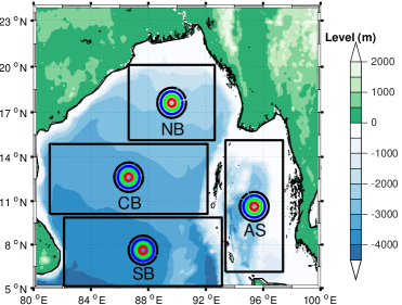
Figure 1: The Bay of Bengal and subregions [Northern Bay (NB), Central Bay (CB), Southern Bay (SB) and Andaman Sea (AS)].

III Circulation in Bay of Bengal

Given its importance to the regional climate, the seasonal circulation of the BoB has been studied quite extensively [see for example, Potemra et al., 1991, Vinayachandran et al., 1996, Schott and McCreary, 2001], and we refer the readers to the aforementioned papers for details. Here, we provide an overview of the subseasonal surface geostrophic circulation to get a feel for the flow that is responsible for advection in the subsequent passive tracer mixing experiments.

III.1 Physical space characterization

On intraseasonal timescales, in the context of geostrophic surface flows, the co-existence of Rossby waves and (nonlinear) eddies is well established throughout the world’s oceans [see for example, Chelton et al., 2007]. In the BoB too, a rich interplay of Rossby waves and eddies has been noted in numerous studies [for example, Shankar et al., 1996, Babu et al., 2003, Kurien et al., 2010, Chen et al., 2012, Nuncio and Kumar, 2012]. It has been suggested that the west coast of the Bay is a critical region for eddy-mean flow interaction with significant baroclinic instability and the production of eddies [Kurien et al., 2010, Chen et al., 2012, Nuncio and Kumar, 2012]. Further, eddies in the BoB have different propagation characteristics in different regions. For example, eddies in the northern and southern Bay (i.e., north of 15^∘N and south of 10^∘N) propagate in southwestward and northwestward directions, respectively. While those in the central Bay tend to move in along the same latitude in a westward direction [Chen et al., 2012].

We begin with Hovmöller plots with respect to longitude of the zonal geostrophic velocity in different seasons of all the four years (meridional velocities show essentially similar features). The longitude spans $80^{\circ}$E to 100^∘E, with the latitude being fixed at the Central Bay (this is the widest portion of the Bay, hence allows for a clear observation of the east-west movement of disturbances), specifically, $12.125^{\circ}$N. As seen in Figure 2, throughout the year we observe southeast to northwest tilted coherent structures. The tilts are fairly steady across the years and yield a westward phase speed of approximately 8-12 $cm/s$, consistent with prior estimates from the central BoB [Killworth et al., 1997, Chelton et al., 2007, Chen et al., 2012]. Interestingly, these cohesive southeast to northwest tilting structures, or wave packets, also appear to exhibit episodic eastward migration with systematic positive (red) and negative (blue) anomalies. Specific examples are : March to July between 85^∘E to 95^∘E in 2010, February to May around 85^∘E and October to December between 85^∘E and 90^∘E in 2011, October to December between 85^∘E to 90^∘E in 2012 and February to May around 85^∘E in 2013. These suggest a small eastward group velocity associated with these wave packets. We have also constructed Hovmöller plots of the zonal velocity with respect to latitude (not shown), these showed a fairly mixed behavior with sporadic instances of northward and southward tilts. By and large, the movement of disturbances in the East-West direction in the Bay is more pronounced and systematic as compared to North-South migration.

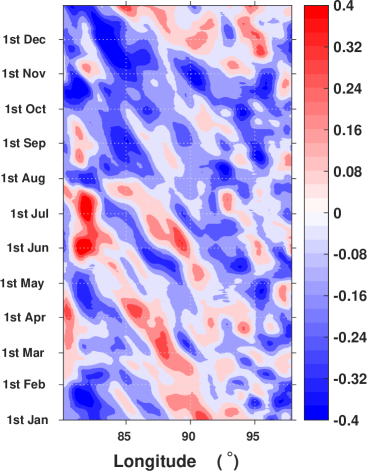
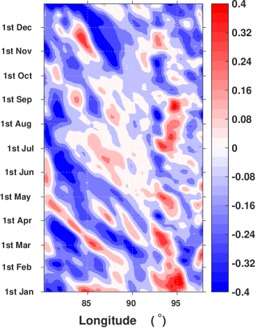
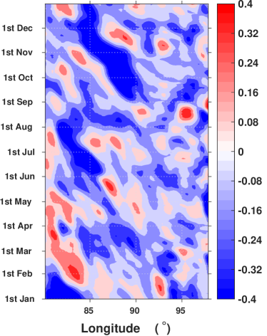
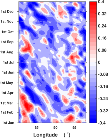
Figure 2: Panels (a), (b), (c) and (d) show Hovmöller diagrams of the zonal geostrophic velocity in 2010, 2011, 2012 and 2013, respectively. The plots are from a longitude of 80^∘E to 100^∘E in the BoB, the cross section is taken near the widest portion of the central Bay at 12.125^∘N

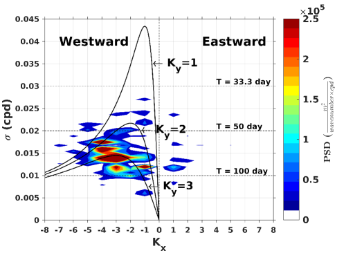
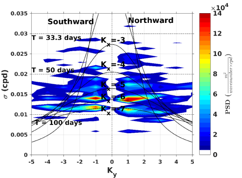
Figure 3: Wavenumber-frequency plots of SLA. Panels (a) and (b) show $\sigma-K_{x}$, averaged over 14^∘N-15^∘N and $\sigma-K_{y}$, averaged over 89.5^∘E-90.5^∘E, respectively. Solid black lines are theoretical linear Rossby wave dispersion curves.

III.2 Spectral space characterization

To get a feel for the scale and time period of these disturbances we move to spectral space and compute wavenumber-frequency diagrams of the sea level anomaly (SLA) constructed from MADT-H. The climatological mean has been removed from the data to construct the SLA and then it is subjected to a 30-120 day band pass Lanczos filtering, with number of coefficient equals to 100. The results presented are averaged over a latitude band from 14.125^∘N to 15.125^∘N (through the central and widest longitudinal extent of the Bay, and for consistency with the Hovmöller plots). As seen in Figure 3, we note strong spectral peaks spread over $|k_{x}|\approx 1-5$ for $k_{x}<0$, with time periods ranging from about 35 to 100 $days$. The three solid curves shown in Figure 3 correspond to the dispersion relations of baroclinic Rossby modes given by,

$$\sigma=-\frac{\beta k_{x}}{{k_{x}}^{2}+{k_{y}}^{2}+\frac{1}{L_{R}^{2}}},\textrm{for }k_{y}=1,2,3.$$ (1)

Here, $k_{x}$ and $k_{y}$ are the zonal and meridional wavenumber and $L_{R}$ is the Rossby radius of deformation. The wavenumbers have been normalized by the length of the BoB which is equal to 1800 $km$ (72 $\times$ 1/4 ^∘) at 15^∘N. The typical value of $L_{R}$, lies between 50-100 $km$ over the latitudes spanned by the Bay [Chelton et al., 1998]. In fact, following Stammer [1997], we estimated an “eddy length scale” from zero crossing of autocorrelation function of the SSH. This estimate (not shown) is somewhat larger than $L_{R}$, and varies from 125-165 $km$ over 18^∘N and 5^∘N. The peaks in the left half of Figure 3 correspond to westward phase speeds, and they appear to be guided by Equation 1. This suggests that these disturbances with westward phase speed are related to baroclinic Rossby waves. Further, the position of the maxima in these diagrams show that there is significant power at scales just smaller than the local deformation scale (maxima of the dispersion curves), thus supporting episodic eastward group velocities noted in the longitudinal Hovmöller plots in Figure 2.

We also computed a dispersion diagram of frequency vs meridional wavenumber, and this is shown in Figure 3. The spectra are averaged over a longitudinal band of 89.625^∘E-90.625^∘E (where we have the largest latitudinal extent of the Bay). The meridional wavenumber has been normalized by the longitudinal cross-section of BoB which is equal to 1675 $km$ (67 $\!\times\!$ 1/4 ^∘) at 90^∘E. We note that the most of the power is distributed between $|k_{x}|\approx 1-5$, with a maximum between $1<|k_{y}|<2$. Also, power appears to be distributed asymmetrically, higher in the northward direction than southwards. Both the wavenumber-frequency plots, $\sigma-k_{x}$ and $\sigma-k_{y}$, have largest power in the temporal band of 60-90 days.

Finally, power spectra are examined to get an idea of the energy associated with the different length and time scales in the geostrophic velocity field. Specifically, we compute kinetic energy spectra and average over 11.125^∘N to 12.125^∘N which resolves largest zonal scales in the Bay. In a similar manner, spectra for meridional wavenumber have been averaged over 89.675^∘E to 90.675^∘E (again, these particular longitudes are chosen to resolve the largest meridional scales in the Bay). The slopes of the spectra, as seen in the first panel of Figure 4, are all close to a $-3$ power-law between approximately 100 $km$ and 250 $km$ in both the zonal and meridional directions. This is agreement with a forward enstrophy cascading regime of surface geostrophic currents from about 200 $km$ to 100 $km$ in the global open oceans [see, for example, the detailed discussion in Khatri et al., 2018]. The temporal spectrum is estimated by calculating the spectrum at each grid point and then averaging. This is done for each year and the results are presented in log-log and variance preserving form in the second and third panels of Figure 4, respectively. The variance preserving form, in agreement with the wavenumber-frequency plots, shows relatively isolated peaks at scales longer than 30 $~{}days$. Further, the log-log plot shows signs of an approximate power-law, with a $-3$ exponent, for time scales that range from about 10-30 $days$. The match in temporal and spatial spectral exponents suggests that Taylor’s hypothesis appears to hold at these scales; specifically, using an annual average speed of 0.2 $m/s$, a spatial scale of 200 $km$ maps to approximately 10 $days$ [see, for example, Ferrari and Wunsch, 2010, Suhas and Sukhatme, 2015]. Note that, given the approximate ten day frequency of repeat satellite passes in AVISO, periods below two weeks suffer from aliasing, and the spectra at these smaller timescales are likely to be unreliable [Arbic et al., 2012]. Taken together, the spatial and temporal spectra suggest an uninterrupted distribution of power across mesoscales and from intraseasonal to weekly time scales, respectively.

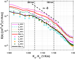
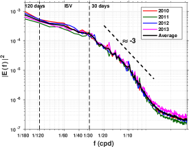
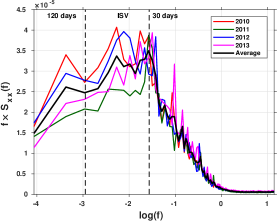
Figure 4: Kinetic energy spectra. Panel (a) shows meridional and zonal wavenumber spectra averaged over 11.125^∘N-12.125^∘N and 89.625^∘E-90.625^∘E, respectively. Panels (b) and (c) contain temporal spectra vs $f$ (frequency) in log-log scale and variance preserving form, respectively. Spectra are estimated at each grid point and then averaged.

IV Mixing of Passive Tracers

As demonstrated, geostrophic flow in the BoB has a multiscale character in both space and time. Specifically, there is strong seasonal dependence of the surface flow [for example, current disruption and reversal, Vinayachandran et al., 1996, Schott and McCreary, 2001], along with significant subseasonal variability consisting of geostrophically balanced disturbances that exhibit predominantly westward phase speeds and align quite well with the dispersion curves for baroclinic Rossby waves. All together, the flow provides a rich playground for the mixing of passive fields. As it happens, aperiodic Rossby waves by themselves have been examined in detail as idealized models of chaotic mixing [see, for example, Pierrehumbert, 1991]. The principal tool used in these mixing calculations is the Lagrangian advection of parcels. This is done using a Runge Kutta fourth order (RK4) scheme. Further, given that the data is on a fixed grid, the flow has been interpolated by a bilinear interpolation scheme.

As our measures of mixing are Lagrangian in nature, it is worth identifying the limits imposed on the calculations due to the resolution of the altimeter data. In general, as discussed by Bartello [2000], coarse velocity field data performs satisfactorily with regard to passive advection when its kinetic energy spectrum follows a $-3$ power-law. Of course, finer scale data can improve quantification of Lagrangian measures [Beron-Vera, 2010]. As seen in Figure 4, currents in the Bay follow this scaling over a range of approximately 100 to 250 $km$. But, the situation is complicated at smaller scales. Specifically, at the ocean’s surface, scales below approximately 100 $km$ (depending on the region in consideration) have a significant contribution from the divergent component of the flow [Capet et al., 2008, Bühler et al., 2014, 2017, Qiu et al., 2017], and spectra at these scales smaller also show signs of flattening to shallower power-laws [Callies and Ferrari, 2013]. Not only is the altimeter derived geostrophic data attenuated by filtering below scales of approximately 100 $km$ [see, for example, Arbic et al., 2013, Dufau et al., 2016], it is unlikely to be a dominant contributor to the actual surface currents. Thus, caution must be exercised in interpreting Lagrangian measures computed from purely geostrophic data below a scale of approximately 100 $km$.

IV.1 A Sign of Chaos

We begin with a simple numerical experiment where the BoB is divided into zonal and longitudinal sections. Each band is approximately 2^∘ wide and is identified by a separate color as seen in the first two panels of Figure 5. Parcels in each band retain their color and are advected for about six weeks. Such experiments give a basic feel for the mixing processes at work [see, for example, Pierrehumbert and Yang, 1993]. Snapshots of the scalar field are shown every two weeks in Figure 5. We notice that within the first two weeks, the bands are distorted and form extended filaments and whorls. In fact, the boundaries between the different colors evolve towards highly complicated contours. This process continues with the repeated wrapping around of progressively thinner scalar filaments, i.e., a cascade of tracer variance to small scales. Indeed, the geometric picture that emerges is that of chaotic advection of a tracer field [Ottino, 1989], and by week six it is quite difficult to distinguish between the longitudinal and latitudinal bands. With this qualitative picture in mind, we now proceed to more quantitative measures of mixing in the BoB.

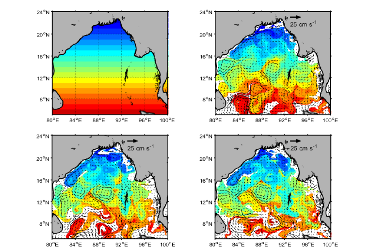
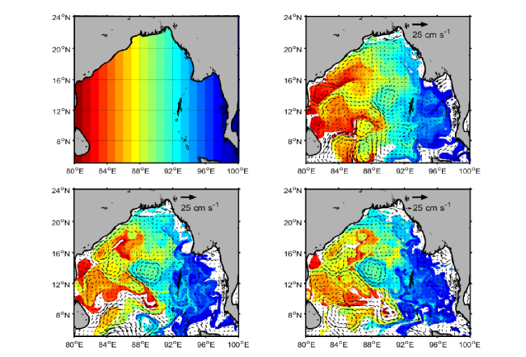
Figure 5: The stirring of latitudinal (first four panels) and longitudinal (last four panels) bands by geostrophic currents from September to October 2012. Snapshots are shown every two weeks for six week long advection.

IV.2 Finite Time Lyapunov Exponents

A fundamental quantitative characteristic of a chaotic flow is its Lyapunov exponent, this is defined as the exponential rate of separation, averaged over infinite time, of fluid parcels with initial infinitesimal separation [Benettin et al., 1980]. For practical problems, the limit of time tending to $\infty$ is not feasible, and the notion is generalized to the so-called Finite Time Lyapunov Exponents (FTLE, $\lambda_{T}$). Specifically,

$$\lambda_{T}(\tau)=\lim_{r(0)\to 0}\frac{1}{\tau}\log\frac{r(\tau)}{r(0)}.$$ (2)

For non-autonomous flows, the FTLE is essentially a measure of integrated strain along a parcel’s trajectory. Here, $\lambda_{T}(\tau)$ is calculated from the logarithm of the largest eigenvalue of $M^{T}M$, where $M$ is the deformation matrix obtained by integrating the Jacobian of the flow along a trajectory [details can be found in, Haller, 2002, Abraham and Bowen, 2002, Waugh et al., 2005]. A finite difference scheme is employed to compute the Jacobian and its traceless component is used to obtain $M$, which ensures that $\lambda_{T}(\tau)$ is positive.

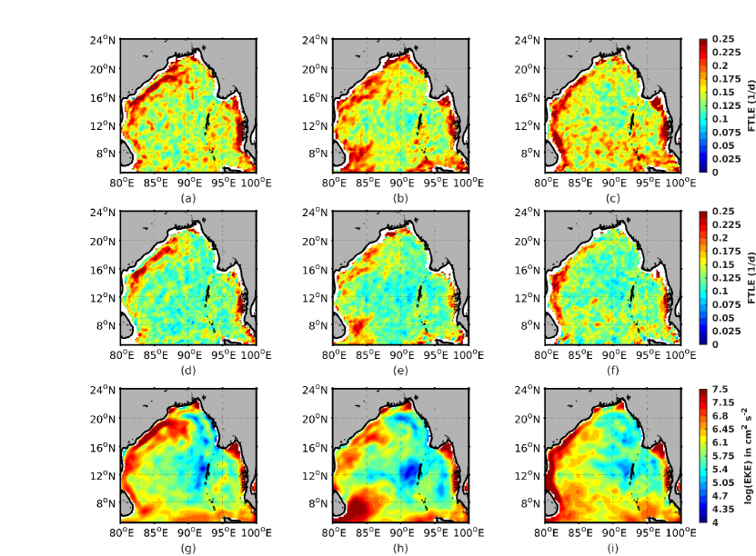
Figure 6: Panels (a) and (d) show the FTLE for 5 and 10 days in FMA, (b) and (e) for JJAS, (c) and (f) for the OND season. Panels (g), (h) and (i) show the corresponding eddy kinetic energy for FMA, JJAS and OND seasons, respectively.

FTLEs are estimated for $\tau=5,10,15$ and 20 $days$ for all the months of four years. Proceeding seasonally, we have averaged FTLEs for Feb-Mar-Apr (FMA), Jun-Jul-Aug-Sep (JJAS) and Oct-Nov-Dec (OND). Further, the average is for seasons from all four years of data (2010-2013). Figure 6 shows the resulting seasonal FTLE maps for $\tau=5$ and 10 $days$. Positive values of the FTLE indicate chaotic behavior over most regions of the Bay. In the premonsoon season (FMA), the FTLEs after 5 and 10 $days$ are high along the western boundary and the northern Bay with values of approximately 0.15-0.3 $day^{-1}$ and 0.1-0.2 $day^{-1}$, respectively. Interestingly, for $\tau=10$ $days$, the southwest portion of the Bay (near the Andaman Sea) also shows strong chaotic mixing. The picture changes in the monsoon period (JJAS), with higher FTLEs on the western boundary moving systematically equatorward. Another notable feature of JJAS is the emergence of a localized pocket of high FTLEs off the east coast of Sri Lanka, this enhanced mixing during the monsoon is due to the so-called Sri Lankan dome [Vinayachandran and Yamagata, 1998]. Further, the central regions of the Bay show relatively smaller FTLEs, suggestive of kinematic barriers to basin wide mixing between the eastern and western portions of the Bay. This is consistent with Figure 5 where we saw stretching and folding at scales smaller than the basin size. Finally, in OND, the southern part of the Bay lights up with high FTLEs. A close inspection of the maps in OND shows signs of a ring of high FTLEs between 85^∘-90^∘E and 8^∘-12^∘N, a feature sometimes referred to as the BoB dome [Vinayachandran and Yamagata, 1998]. The northwest boundary is now relatively quiescent with low FTLE values. Overall, we see a seasonal cycle in mixing with rapid stirring progressively moving from the northern to southern Bay, from pre-monsoonal to post-monsoonal periods, respectively. Further, the eddy kinetic energy (EKE) in the Bay (where eddies are defined as deviations from a climatological 4 year mean) in each season is also shown in the third panel of Figure 6. Clearly, the EKE map aligns quite closely with that of the FTLEs in each season. This has been noted on global [Waugh and Abraham, 2008], as well more local scales [Waugh et al., 2005], in the world’s oceans.

At a fundamental level, the action of a chaotic flow on the transport or evolution of a passive field requires a knowledge of the probability density function of the FTLEs [see, for example, Balkovsky and Fouxon, 1999, Sukhatme and Pierrehumbert, 2002, Fereday and Haynes, 2004, Haynes and Vanneste, 2004]. The histogram of FTLEs is shown in the first panel of Figure 7. This distribution reflects the spatially non-uniform nature of stirring induced by the geostrophic currents in the Bay. Indeed, the slow right tail represents regions that experience rapid mixing, while the left tail is indicative of slow rates of stirring. Also, the shape of the distribution changes for different $\tau$. Specifically, the histogram becomes taller (mean decreases) with more of a stretched exponential tail for larger $\tau$. In essence, the non-uniformity of mixing is highlighted more starkly for longer time intervals. Even though the regions of strong mixing vary from season to season, as seen in the second panel of Figure 7, there is not much of a seasonal dependence in the FTLE distributions, i.e., the Bay is non-uniformly chaotic throughout the year. This can also be seen in Figure7, which shows a daily time series of the mean FTLE over the Bay through the year. The average stirring rate is quite uniform through the year, though there is a marginal increase during the post monsoonal months.

For consistency with other parts of the world’s oceans [Waugh and Abraham, 2008, Waugh et al., 2012], we note that a Weibull distribution (shown in the fourth panel of Figure 7) accurately fits the FTLE histogram normalized by the mean FTLE. The specific expression plotted in Figure 7 is,

$$P(\lambda)=\frac{b}{a}{(\frac{\lambda}{a})}^{b-1}\exp(-\frac{\lambda^{b}}{a^{b}}),$$ (3)

with $a=1.15$ and $b=1.95$.

IV.3 Relative Dispersion

Another commonly used mixing diagnostic is relative dispersion [RD; see for example, LaCasce, 2010]. This is defined as,

$$\langle R^{2}(t)\rangle=\frac{1}{N(N-1)}\sum_{i\neq j}{R^{2}}_{ij}(t)$$ (4)

where, $\langle R^{2}(t)\rangle$ is the mean relative dispersion of an ensemble of $N$ pairs having the same initial separation with random orientation. RD, along with notions such as normal or anomalous diffusion, helps in quantifying the homogenization of tracers [see, for example, Weeks et al., 1996, LaCasce and Speer, 1999, Sukhatme, 2005, for ideal, oceanic and atmospheric applications, respectively]. Recently, Waugh et al. [2012] have compared RD and FTLEs, and highlighted how they explore different aspects of the mixing process. Quite starkly, even in the case when the FTLE distribution collapses to a single point, the RD exhibits a wide spread [Waugh et al., 2012].

In practice, we advected 1000 pairs of parcels at a given grid location for 90 $days$ starting on the first day of each month in all the four years. Two suites of experiments were conducted with pairs in a circle that are initially 10 and 25 $km$ apart, respectively. The evolution of RD with these two initial separations is shown in Figure 8 and 8. At small scales, the advecting flow is a smoothly interpolated geostrophic flow, hence the observed exponential separation is not surprising. As discussed earlier, at small scales (below approximately 100 $km$, depending on the region in consideration), the surface ocean flow appears to have a relatively shallow kinetic energy spectrum [Callies and Ferrari, 2013], and a significant divergent component [Capet et al., 2008, Bühler et al., 2014, Qiu et al., 2017]. In fact, pair separation on the order of a few $km$, estimated using drifter data from the Gulf of Mexico, appears to conform with the classic Richardson $\langle R^{2}\rangle\sim t^{3}$ prescription [Poje et al., 2017]. Indeed, it would be interesting to ascertain the behavior of RD in the 10-100 $km$ range via high resolution surface ocean models.

At scales between 100 and 250 $km$, we observe that the RD is reasonably well approximated by a power-law growth in time. While we anticipate exponential separation in an enstrophy cascading regime, it should be remembered that this is under the assumption of an inertial range with a constant enstrophy flux [Lin, 1972]. Computation of the enstrophy flux using altimeter data does show a dominant forward enstrophy regime at these scales, but the enstrophy flux is not constant, and is actually scale dependent [Khatri et al., 2018]. Therefore, the power-law growth of RD is not inconsistent with a forward enstrophy transfer regime. Finally, at scales larger than 250 $km$, the growth of RD slows down and tends to $\langle R^{2}\rangle\sim t$, indicative of eddy diffusive behavior. This is seen in the emergent flat portion of a compensated RD plot (for the 25 $km$ initial separation case) beyond approximately 70 $days$ of evolution as shown in Figure 8.

As with the FTLEs, the distribution of RD at a given time is of importance in assessing the non-uniformity of mixing. The distribution of RD (actually, the square root of RD, normalized by its rms value), at various times, when the mean square root RD lies between 100 and 250 $km$ is shown in Figure 8 and 8 for 10 and 25 $km$ initial separations, respectively. Quite clearly, the distributions are not Gaussian, rather they show signs of a log-normal behavior. Spatial maps of the mean RD are presented in Figure 9. In the premonsoon period (FMA), the western coastline supports rapid pair dispersal, while the southern Bay shows subdued RD values. In the monsoon season (JJAS), high RD shifts slightly off the western coast, and in addition, rapid dispersion picks up in the parts of the southern and eastern Bay. Finally, in the postmonsoon period (OND), along with the west coast, much of the southern and eastern Bay lights up with high RD values. Interestingly, all through the year, the central Bay is characterized by low RD values, and this also points to a local or eddy scale mixing, rather than basin wide homogenization.

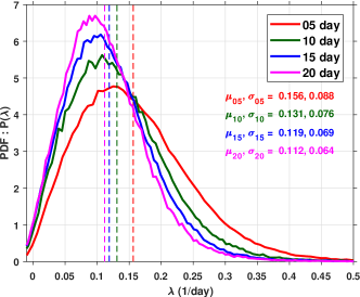
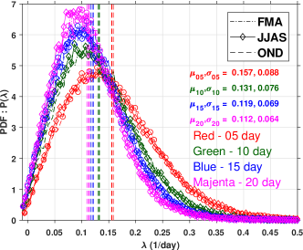
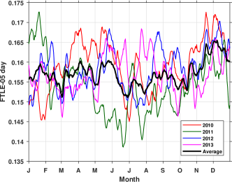
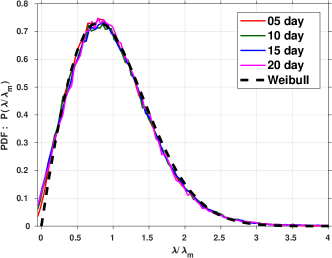
Figure 7: Histogram of FTLEs (with different increments) over the Bay; (a) whole year (b) in different seasons. Panel (c) shows the five day mean FTLE time series through the year. Panel (d) shows a fit to the FTLE distribution by a Weibull distribution (normalized by mean $\lambda$ to the FTLE histogram for different $\tau$.

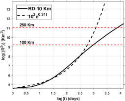
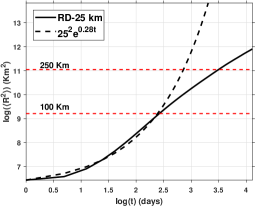
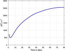
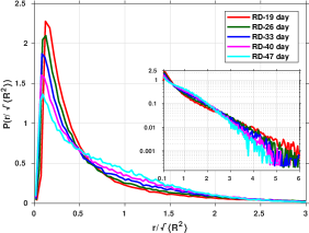
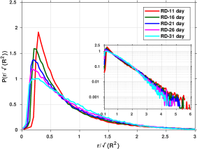
Figure 8: Panels (a) and (b) show the RD with time for initial separations of 10 and 25 $km$, respectively. Panel (c) shows the compensated RD (by $t^{-1}$) as a function of time. Panels (d) and (e) show histograms of the square root of RD (denoted by $r$, normalized by its rms value) at different days when the mean RD is between 100 and 250 $km$.

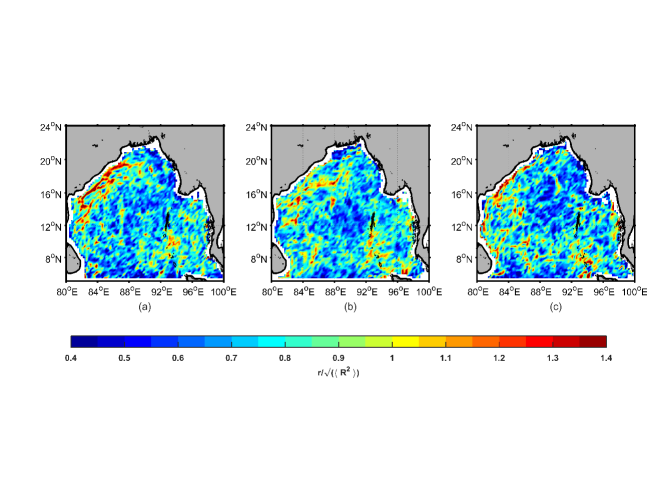
Figure 9: Panels (a), (b) and (c) show maps of the square root RD (normalized by its rms value) at 15 $days$ from an initial cluster of 25 $km$ separation in the premonsoon (FMA), monsoon (JJAS) and postmonsoon (OND) periods, respectively.

IV.4 Finite Size Lyapunov Exponent

For a flow with multiple scales, such as that in the BoB, the Finite Size Lyapunov Exponent (FSLE) is a convenient measure that quantifies the chaotic nature of the flow [Artale et al., 1997, Hernández-Carrasco et al., 2011]. In particular, the FLSE allows one to estimate the scale up to which mixing is chaotic, and beyond which, a diffusive framework is appropriate. From a practical viewpoint, this also allows an estimation of a scale dependent diffusion coefficient [Lacorata et al., 2001].

Following García-Olivares et al. [2007], a set of $M$ tracers with some initial distribution and standard deviation $\sigma$ are followed in time as they are transported by the velocity field. The parameter $\sigma(t)$ is defined as,

$$\sigma(t)={\langle{|x_{i}(t)-\langle x_{i}(t)\rangle|}^{2}\rangle}^{1/2},\textrm{where},$$ (5)

$$\langle x_{i}(t)\rangle\equiv\langle\{x_{i}(t):i=1,2,...M\}\rangle=\frac{1}{M}\sum_{i=1}^{M}x_{i}(t).$$ (6)

We define the initial size of the cluster ${\sigma}_{0}$ according to 5 and 6, and measure the time $T$(${\sigma}_{0}$,r) it takes for the growth from ${\sigma}_{0}$ to ${\sigma}_{1}$ = r $\sigma_{0}$ , $T$($\sigma_{1},r$) the time it takes for the growth from $\sigma_{1}$ to $\sigma_{2}$ = r$\sigma_{1}$, and so on up to the largest scale under consideration (the sub-basin scale). A set of $N$ experiments is then performed with different initial conditions for the cluster of particles $N\gg$ 1, and we calculate the mean time $\tau$ that a cluster with size $\sigma_{j}$ takes to grow by a factor $r$ and the $\langle\cdot\rangle$ operation is the average over the tracer ensemble. This reads,

$$\tau(\sigma_{j},r)=\langle T(\sigma_{j},r)\rangle=\frac{1}{N}\sum_{j=1}^{N}T(\sigma_{j},r).$$ (7)

The FSLE parameter as a function of the scale is then obtained by the following expression,

$$\lambda(x,{\sigma}_{j})=\frac{\log r}{\tau(\sigma_{j},r)},$$ (8)

which is not sensitive to variations in $r$ when it is close to 1+. From the FSLE, we define the Finite Size Diffusion Coefficient (FSDC, $D$) as,

$$D(\sigma)={\sigma}^{2}\lambda(\sigma).$$ (9)

As the cluster size grows, if it is driven by chaos at very small scales ($\ll l_{u}$) and by (eddy) diffusion at very large scales ($\gg l_{u}$), then $\lambda(\sigma)$ has the following asymptotic behavior,

$$\lambda(\sigma)=\begin{cases}{\lambda}_{max},&\text{if}\ \sigma\ll l_{u},\\ \frac{D}{{\sigma}^{2}},&\text{if}\ \sigma\gg l_{u}.\\ \end{cases}$$ (10)

Though, for real world data, as demonstrated in Corrado et al. [2017] in an oceanic setting, there usually exist other intermediate regimes for $\lambda(\sigma)$.

Practically, for calculating the FSLE, a cluster with 10000 parcels was released at each grid location, and these were advected in time for approximately 60 $days$. In fact, we have chosen a cluster whose initial standard deviation is 25 $km$ and followed the parcels till the standard deviation increases by a factor of 1.2. The size of the initial cluster is varied from 25 $km$ to approximately 300 $km$. This experiment was repeated for every year, and an average was taken over all years.

The behavior of the FSLE with cluster size can be seen in Figure 10. As with RD, the smoothly interpolated flow results in an exponential separation, i.e., a relatively flat FSLE, for scales below approximately 100 $km$. For the NB and SB an eddy-diffusive regime is observed for scales greater than 200-250 $km$ (via a $-2$ scaling of the FSLE in Figure 10). At intermediate scales, i.e., 100 to 250 $km$, the FSLE transitions between these two end regimes. The behavior of the Andaman Sea region is somewhat different with the diffusive regime emerging earlier between 150 and 200 $km$, itself. This overall picture is consistent with the calculated “eddy length scale” and the local chaotic mixing seen in Figure 9. Interestingly, the CB is quite distinct in that the FSLE never really transitions to an eddy-diffusive regime. It is possible that, especially in the intermediate regime, finer data may yield different power-laws as seen by Corrado et al. [2017] in other parts of the world’s oceans. An estimation of a scale dependent diffusion co-efficient, the FSDC, is presented in Figure 10. It is interesting to note that the FSDC scales as a power-law with cluster size (exponent of 1.73), this is potentially a useful reference which provides a resolution-diffusivity relation for use in models. At large scales, for the NB and SB, the eddy diffusivity is approximately $10^{4}$ $m^{2}/s$. In the Andaman Sea region, the value is lower and is near $6\times\!10^{3}$ $m^{2}/s$. These numbers are higher (by a factor of 2) than the minimum Osborn-Cox eddy diffusivity estimates as determined by Abernathey and Marshall [2013] (see in particular the Bay of Bengal in their global Figure 5), but are of the same order as diffusivities estimated via FSLEs in other parts of the world’s oceans [Corrado et al., 2017].

The seasonal mean picture of FSLEs (within the chaotic regime) is shown in Figure 11. As with the seasonal picture from the FTLEs, high values of the FSLE show equatorward movement from FMA, through JJAS into OND. Note that the mouth of the river Ganga-Brahmaputra basin and Irrawaddy catchment area show high FSLE in JJAS and OND season. Signs of the Sri Lankan and BoB domes can also be seen in the FSLE maps in JJAS and OND, respectively. Also, low FSLE values can be seen in the CB region throughout the year which are consistent with a partition that inhibits basin scale mixing.

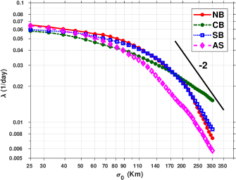
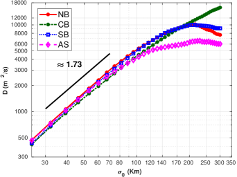
Figure 10: Panels (a) and (b) show FSLE and eddy diffusivity as a function of initial cloud size with expansion factor $r=1.2$ for the Northern Bay, Central Bay, Southern Bay and Andaman Sea.

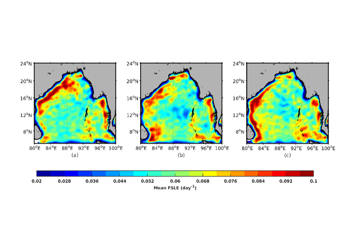
Figure 11: Panels (a), (b), (c) show the mean FSLE for FMA, JJAS, OND seasons respectively. This is an average over all four years of altimetry data.

V Analysis of a single fresh water mixing event

As mentioned earlier, a significant amount of surface fresh water enters the Bay in the postmonsoon season from the Ganga-Brahmaputra (GB) catchment [Papa et al., 2012, Chaitanya et al., 2014], and plays an important role in its surface salinity budget [Howden and Murtugudde, 2001]. This inflow from GB progresses southward and is largely confined to the western side of the Bay [referred to as a river in the sea, Chaitanya et al., 2014]. The fate of this fresh water, including its advection, and homogenization with a more salty environment has been analyzed in detail [Akhil et al., 2014]. Indeed, it appears that the fresh water maintains its identity for an extended period and finally extended tongues become saltier in the southern Bay [Benshila et al., 2014, Akhil et al., 2014]. Lagrangian salinity change maps from data from August to October of 2013 also show an increase in the saltiness with southward advection [Mahadevan et al., 2016]. Though it should be kept in mind that some fresh water retains its identify for a prolonged period and its transport to remote regions in the Indian Ocean has been documented [Sengupta et al., 2006].

Taking advantage of satellite data from 2015, stirring of the salinity field by eddies in the postmonsoon season has been recently explored by Fournier et al. [2017]. Here, we highlight role of eddies off the eastern coast on India in preserving the identity of fresh water. In particular, we showcase a particular eddy that formed around the end of October and lasted to the end of November in 2015. The salinity field along with quivers of the geostrophic flow on October 25 are shown in the first panel of Figure 12. The eddy is well formed and spans the approximate region 16-19^∘N to 85-88^∘E, with a slight northwest-southeast tilt. The second panel of Figure 12 shows a passive tracer initialized to have the same value as the salinity field, along with contours of 5 day FTLEs. Note that a fair amount of fresh water (blue) is contained within the eddy. The two panels of Figure 12 show maps of FTLEs (15 $day$) and FSLEs ($r=1.2$) in this part of the Bay. Quite clearly, the region inside the eddy is characterized by relatively low FTLEs/FSLEs while it is surrounded by a high FTLE/FSLE ring. Also, note that inside the eddy, the interior rim has lowest FTLEs while the central region has relatively higher stirring rates. Thus, much like the scenario described by Rhines and Young [1983], we expect a tracer to be well mixed within an eddy, but not communicate significantly (or, possibly on a slower timescale) with the “external” Bay.

Fifteen days later, as seen in the first panel of Figure 13, low salinity water is retained within the eddy. The passive tracer, advected via the geostrophic flow in these fifteen days is shown in the second panel of Figure 13. While the bulk of “fresh” passive tracer is in the eddy, long filaments that initially comprised of material localized on the outer side of the eddy, extend southwards up to 12^∘N and westward to the coast. These narrow filaments are not seen in the actual salinity field, and have most likely been homogenized via the more salty environment — possibly due to strong vertical mixing [Benshila et al., 2014, Akhil et al., 2014]. Finally, another fifteen days later, on November 24 (Figure 13), the passive and salinity fields compare favorably, even though the eddy itself has deformed considerably. In fact, it is now squeezed along the coast into a northeast-southwest orientation, and fresh water begins to be strained out of its southwest boundary. Remnants of ejected filaments from the edges of the eddy that are seen in the passive field are absent in the salinity data, presumably also having being been homogenized to more salty levels.

Thus, in this period of one month, fresh water trapped inside the eddy is shielded by means of kinematic transport barriers that are clearly delineated by the FTLE and FSLE maps. In addition, this eddy trapped fresh water stays in place rather than being rapidly advected in a southward direction. On comparison with the passive tracer, we note that ejected passive filaments are not seen in the fresh water signature, thus highlighting the role of the kinematic barriers in the preservation of fresh water on this monthly timescale.

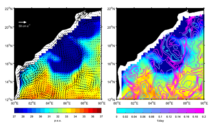
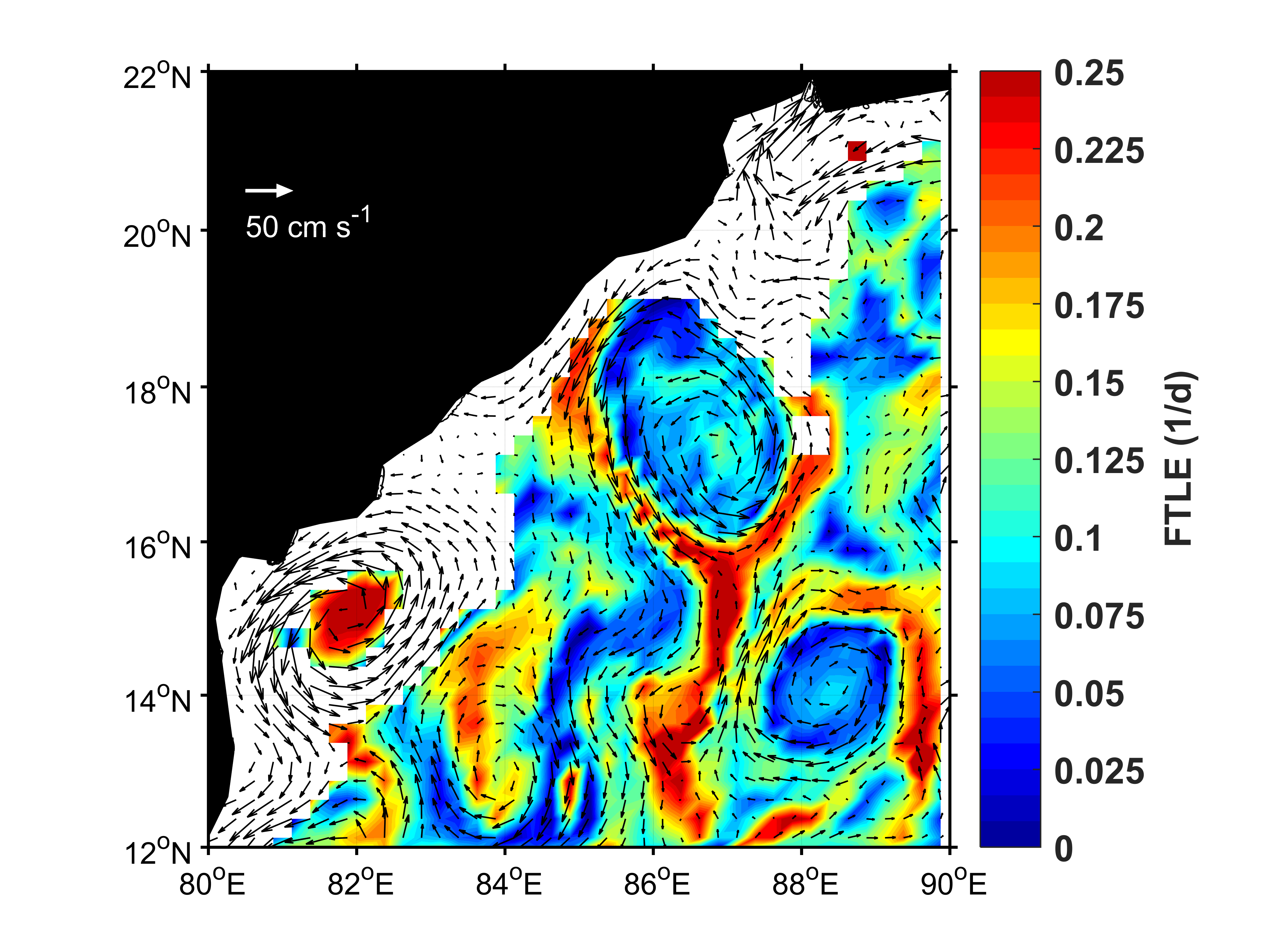
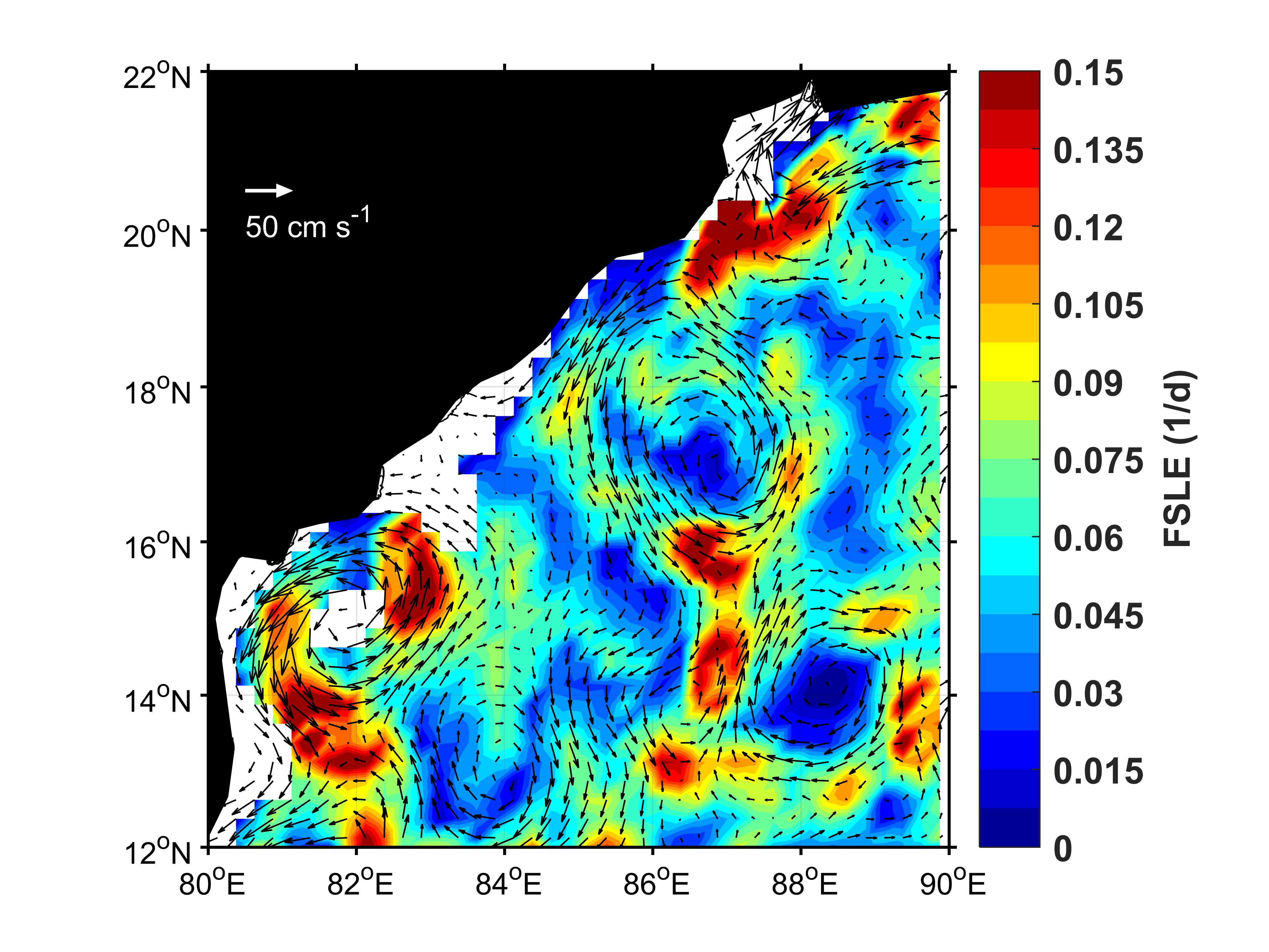
Figure 12: Panel (a) shows salinity map with velocity quivers (left) and FTLE-05 day contours overlaid onto passive scalar field (right) on 25/10/2015. Panel (b) shows the spatial map of FTLE-15 day (left) and FSLE (right) on 25/10/2015.

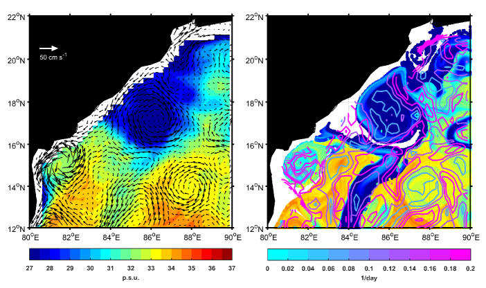
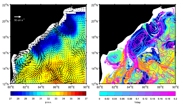
Figure 13: Panels (a) and (b) shows salinity map with velocity quivers (left) and FTLE-05 day contours overlaid onto passive scalar field (right) on 08/11/2015 and 24/11/2015, respectively.

VI Summary and Discussion

Using surface geostrophic currents derived from altimetry data, we studied mixing along the surface of the Bay of Bengal. In particular, our primary focus was on mixing that takes place on intraseasonal scales. To begin with, we examined the flow by means of Hovmöller plots and wavenumber-frequency diagrams. It was seen that the geostrophic currents in the Bay are dominated by westward progressing disturbances that have temporal scales between 50 and 100 $days$. In fact, the power in these systems aligned well with the theoretical dispersion curves for linear baroclinic Rossby waves. Interestingly, some of these have length scales that are smaller than the local deformation scale, and show an eastward group velocity which was noted in the Hovmöller plots. Temporal and spatial power spectra were seen to follow approximate power-laws ($-3$ scaling, from 100-250 $km$ and 10-30 $days$, respectively) and suggested an uninterrupted distribution of power across length and subseasonal time scales.

The advection of latitudinal and longitudinal bands by the multiscale geostrophic flow immediately hinted at the presence of chaotic mixing. In particular, the repeated folding and filamentation of stripes brought forth a complicated geometry to the mixing process, and by the end of approximately six weeks, it was difficult to distinguish between the two initial conditions. In addition, mixing was not basin wide but was seen to be restricted to the scale of eddies.

A more quantitative measure of mixing was provided by the FTLEs. Maps of the FTLEs suggested an equatorward movement of regions of enhanced mixing from pre-monsoonal to post-monsoonal periods. In each season, the central Bay had low FTLE values, suggestive of the presence of kinematic barriers that were consistent with the eddy scale of mixing noted above. Specific seasonal features, such as the appearance of the Sri Lankan dome in the monsoon, were captured by high FTLE pockets. Also, overall, the spatial maps of FTLEs were in tune with those of eddy kinetic energy. Variations in FTLEs are known to be important in determining the outcome of advection-diffusion on passive fields; here, the non-uniform nature of surface mixing in the Bay was manifest in the histograms of FTLEs that had long tails and their shape, and as in other parts of the world’s oceans, was captured well by a Weibull distribution. In terms of a domain average, the FTLE for a week’s increment was approximately 0.1 $day^{-1}$, while the spread captured by the histogram ranged up to $0.5$ $day^{-1}$. In addition, with longer time increments, the distribution of FTLEs became taller (and smaller mean), but with progressively more stretched exponential like tails. Thus, the non-uniformity of mixing was further highlighted at longer time intervals.

The relative dispersion (RD) of parcels provided a complimentary view to the FTLEs. Below 100 $km$, the smoothly interpolated nature of the data results in pair separation that was exponential in time. From 100 to 250 $km$, i.e., the RD followed a power-law in time, which is consistent a forward enstrophy transfer regime, but with a variable enstrophy flux. At larger scales, the pair separation took on an eddy-diffusive growth, i.e., $\langle R^{2}\rangle\sim t$. Consistent with the FTLEs, seasonal mean maps showed a southward progression of high RD, and a suppressed dispersion in the central Bay throughout the year.

FSLEs were then estimated for the Bay, these provide a quantitative measure of the scale up to which tracers experience chaotic mixing. Averaging the growth of clusters in different months, and across all four years, the FSLE followed theoretical expectations. In particular, the FTLE was relatively constant (up to 100 $km$), transitions (from 100 to 250 $km$) and then enters an eddy-diffusive regime (above 250 $km$). The Andaman Sea was seen to enter an eddy-diffusive regime at relatively smaller scales (150 $km$) while the central showed no signs of this transition. Overall, in agreement with FTLEs and latitudinal (longitudinal) stripe experiments, chaotic mixing takes place within eddies. Beyond the eddy scale, the $-2$ power-law suggested an eddy diffusive behavior (except in the central Bay), with each eddy acting independently and inducing a random walk of the tracer. The large scale eddy-diffusivity estimated from the FSLE plots was about $10^{4}$ $m^{2}/s$ in the northern and southern Bay, and approximately $6\times 10^{3}$ $m^{2}/s$ in the Andaman Sea region. Interestingly, before the emergence of an eddy-diffusive regime, the finite size diffusion coefficient showed a similar power-law behavior in all regions of the Bay (exponent of 1.73 with cluster size). These estimates can be used as a guideline for ocean models, being run at a given resolution, that hope to capture the stirring at the surface of the Bay in an accurate manner.

Finally, from a global perspective of mixing in the Bay, we moved to the analysis of a single fresh water mixing episode. Guided by satellite salinity data in 2015, we demonstrated how an eddy in the western Bay helps preserve the identity of post-monsoonal fresh water from the Ganga-Brahmaputra river mouth. In particular, FSLE and FTLE maps clearly delineated kinematic boundaries that aid in mixing within eddies, but prevent the intermingling of fresh water within an eddy with the saltier external Bay over the timescale of a month. Thus, while eddies stir the salinity field on a large scale, they also help maintain the freshness of water trapped within themselves.

VII Acknowledgement

The authors would like to thank AVISO and JPL for making MADT-H-UV and SMAP salinity data freely available. The authors would like to express their gratitude to Dr. Debasis Sengupta, Dr. Anirban Guha and Dr. Amit Tandon for helpful discussions and technical advice. We also thank the Divecha Centre for Climate Change, IISc for financial support.

References

- Abernathey and Marshall [2013] R. Abernathey and J. Marshall. Global surface eddy diffusivities derived from satellite altimetry. Journal of Geophysical Research, 118:901–916, 2013. doi: 10.1002/jgrc.20066.
- Abraham [1998] E. Abraham. The generation of plankton patchiness by turbulent stirring. Nature, 391:577–580, 1998.
- Abraham and Bowen [2002] E. R. Abraham and M. M. Bowen. Chaotic stirring by a mesoscale surface-ocean flow. Chaos: An Interdisciplinary Journal of Nonlinear Science, 12(2):373–381, 2002.
- Akhil et al. [2014] V. Akhil et al. A modeling study of the processes of surface salinity seasonal cycle in the Bay of Bengal. Journal of Geophysical Research, 119(6):3926–3947, 2014. doi: 10.1002/2013JC009632.
- Arbic et al. [2012] B. Arbic, R. Scott, G. Flierl, A. Morten, J. Richman, and J. Shriver. Nonlinear cascades of surface oceanic geostrophic kinetic energy in the frequency domain. Journal of Physical Oceanography, 42:1577–1600, 2012. doi: 10.1175/JPO-D-11-0151.1.
- Arbic et al. [2013] B. K. Arbic, K. L. Polzin, R. B. Scott, J. G. Richman, and J. F. Shriver. On eddy viscosity, energy cascades, and the horizontal resolution of gridded satellite altimeter products. Journal of Physical Oceanography, 43(2):283–300, 2013. doi: 10.1175/JPO-D-11-0240.1.
- Aref [1984] H. Aref. Stirring by chaotic advection. Journal of Fluid Mechanics, 143:1–21, 1984.
- Aref et al. [2017] H. Aref et al. Frontiers of chaotic advection. Reviews of Modern Physics, 89, 2017. doi: 10.1103/RevModPhys.89.025007.
- Artale et al. [1997] V. Artale, G. Boffetta, A. Celani, M. Cencini, and A. Vulpiani. Dispersion of passive tracers in closed basins: Beyond the diffusion coefficient. Physics of Fluids, 11:3162–3171, 1997.
- Babu et al. [2003] M. Babu, Y. Sarma, V. Murty, and P. Vethamony. On the circulation in the Bay of Bengal during northern spring inter-monsoon (March–April 1987). Deep Sea Research Part II: Topical Studies in Oceanography, 50(5):855–865, 2003.
- Balkovsky and Fouxon [1999] E. Balkovsky and A. Fouxon. Universal long-time properties of Lagrangian statistics in the Batchelor regime and their application to the passive scalar problem. Physical Review E, 60(4):4164, 1999.
- Bartello [2000] P. Bartello. Using low-resolution winds to deduce fine structure in tracers. Atmosphere-Ocean, 38:303–320, 2000. doi: 10.1080/07055900.2000.9649650.
- Benettin et al. [1980] G. Benettin, L. Galgani, A. Giorgilli, and J.-M. Strelcyn. Lyapunov characteristic exponents for smooth dynamical systems and for Hamiltonian systems; a method for computing all of them. Part 1: Theory. Meccanica, 15(1):9–20, 1980.
- Benshila et al. [2014] R. Benshila et al. The upper Bay of Bengal salinity structure in a high-resolution model. Ocean Modelling, 74:36–52, 2014. doi: 10.1016/j.ocemod.2013.12.001.
- Beron-Vera [2010] F. Beron-Vera. Mixing by low-and high-resolution surface geostrophic currents. Journal of Geophysical Research, 115:C10027, 2010. doi: 10.1029/2009JC006006.
- Beron-Vera et al. [2008] F. Beron-Vera, M. Olascoaga, and G. Goni. Oceanic mesoscale eddies as revealed by Lagrangian coherent structures. Geophysical Research Letters, 35:L12603, 2008. doi: 0.1029/2008GL033957.
- Boffetta et al. [2001] G. Boffetta et al. Detecting barriers to transport: a review of different techniques. Physica D, 159:58–70, 2001.
- Bühler et al. [2014] O. Bühler, J. Callies, and R. Ferrari. Wave-vortex decomposition of one-dimensional ship-track data. J. Fluid Mech., 756:1007–1026, 2014. doi: 10.1017/jfm.2014.488.
- Bühler et al. [2017] O. Bühler, M. Kuang, and E. Tabak. Anisotropic helmholtz and wave-vortex decomposition of one-dimensional spectra. J. Fluid Mech., 815:361–387, 2017. doi: 10.1017/jfm.2017.57.
- Callies and Ferrari [2013] J. Callies and R. Ferrari. Interpreting energy and tracer spectra of upper-ocean turbulence in the submesoscale range (1–200 km). Journal of Physical Oceanography, 43(11):2456–2474, 2013. doi: 10.1175/JPO-D-13-063.1.
- Capet et al. [2008] X. Capet, J. McWilliams, M. Molemaker, and A. Shchepetkin. Mesoscale to submesoscale transition in the California current system. Part III: Energy balance and flux. Journal of Physical Oceanography, 38(10):2256–2269, 2008. doi: 10.1175/2008JPO3810.1.
- Chaitanya et al. [2014] A. Chaitanya, M. Lengaigne, J. Vialard, V. Gopalakrishna, F. Durand, C. Kranthikumar, C. Amritash, V. Suneel, F. Papa, and M. Ravichandran. Salinity Measurements Collected by Fishermen Reveal a “River in the Sea” Flowing Along the Eastern Coast of India. BAMS, pages 1897–1908, 2014. doi: 10.1175/BAMS-D-12-00243.1.
- Chelton et al. [2007] D. Chelton, M. Schlax, R. Samelson, and R. de Szoeke. Global observations of large oceanic eddies. Geophysical Research Letters, 34:L15606, 2007. doi: 10.1029/2007GL030812.
- Chelton et al. [1998] D. B. Chelton, R. A. Deszoeke, M. G. Schlax, K. El Naggar, and N. Siwertz. Geographical variability of the first baroclinic rossby radius of deformation. Journal of Physical Oceanography, 28(3):433–460, 1998.
- Chen et al. [2012] G. Chen, D. Wang, and Y. Hou. The features and interannual variability mechanism of mesoscale eddies in the Bay of Bengal. Continental Shelf Research, 47:178–185, 2012.
- Cheng et al. [2013] X. Cheng, S.-P. Xie, J. McCreary, Y. Qi, and Y. Du. Intraseasonal variability of sea surface height in the Bay of Bengal. Journal of Geophysical Research: Oceans, 118(2):816–830, 2013.
- Chertkov [1998] M. Chertkov. On how a joint interaction of two innocent partners (smooth advection and linear damping) produces a strong intermittency. Physics of Fluids, 10(11):3017–3019, 1998.
- Corrado et al. [2017] R. Corrado, G. Lacorata, L. Palatella, R. Santoleri, and E. Zambianchi. General characteristics of relative dispersion in the ocean. Scientific Reports, 7:46291, 2017. doi: 10.1038/srep46291.
- Dufau et al. [2016] C. Dufau et al. Mesoscale resolution capability of altimetry: Present and future. Journal of Geophysical Research, 121:4910–4927, 2016. doi: 10.1002/2015JC010904.
- Fereday and Haynes [2004] D. Fereday and P. Haynes. Scalar decay in two-dimensional chaotic advection and Batchelor-regime turbulence. Physics of Fluids, 16(12):4359–4370, 2004.
- Ferrari and Wunsch [2010] R. Ferrari and C. Wunsch. The distribution of eddy kinetic and potential energies in the global ocean. Tellus, 62A:92, 2010.
- Fournier et al. [2017] S. Fournier et al. Modulation of the Ganges-Brahmaputra River Plume by the Indian Ocean Dipole and Eddies Inferred From Satellite Observations. Journal of Geophysical Research, 122:9591–9604, 2017. doi: 10.1002/2017JC013333.
- García-Olivares et al. [2007] A. García-Olivares, J. Isern-Fontanet, and E. García-Ladona. Dispersion of passive tracers and finite-scale Lyapunov exponents in the Western Mediterranean Sea. Deep Sea Research Part I: Oceanographic Research Papers, 54(2):253–268, 2007.
- Haller [2002] G. Haller. Lagrangian coherent structures from approximate velocity data. Physics of Fluids, 14(6):1851–1861, 2002.
- Haynes and Vanneste [2004] P. Haynes and J. Vanneste. Stratospheric tracer spectra. Journal of the Atmospheric Sciences, 61:161–178, 2004.
- Hernández-Carrasco et al. [2011] I. Hernández-Carrasco, C. López, E. Hernández-García, and A. Turiel. How reliable are finite-size lyapunov exponents for the assessment of ocean dynamics? Ocean Modelling, 36(3):208–218, 2011.
- Hernandez-Garcia and Lopez [2004] E. Hernandez-Garcia and C. Lopez. Sustained plankton blooms under open chaotic flows. Ecol. Complex, 1:253–259, 2004.
- Howden and Murtugudde [2001] S. Howden and R. Murtugudde. Effects of rives inputs into the Bay of Bengal. Journal of Geophysical Research, 106(C9):19825–19843, 2001.
- Khatri et al. [2018] H. Khatri, J. Sukhatme, A. Kumar, and M. Verma. Surface ocean enstrophy, kinetic energy fluxes and spectra from satellite altimetry. Journal of Geophysical Research, 2018. doi: 10.1029/2017JC013516.
- Killworth et al. [1997] P. D. Killworth, D. B. Chelton, and R. A. de Szoeke. The speed of observed and theoretical long extratropical planetary waves. Journal of Physical Oceanography, 27(9):1946–1966, 1997.
- Kurien et al. [2010] P. Kurien, M. Ikeda, and V. K. Valsala. Mesoscale variability along the east coast of India in spring as revealed from satellite data and OGCM simulations. Journal of Oceanography, 66(2):273–289, 2010.
- LaCasce [2010] J. LaCasce. Relative displacement probability distribution functions from balloons and drifters. Journal of Marine Research, 68:433–457, 2010.
- LaCasce and Speer [1999] J. LaCasce and K. Speer. Lagrangian statistics in unforced barotropic flows. Journal of Marine Research, 57:245–274, 1999.
- Lacorata et al. [2001] G. Lacorata, E. Aurell, and A. Vulpiani. Drifter dispersion in the Adriatic Sea: Lagrangian data and chaotic model. Annales Geophysicae, 19:121–129, 2001.
- Lebonnois et al. [2001] S. Lebonnois, D. Toublanc, F. Hourdin, and P. Rannou. Seasonal Variations of Titan’s Atmospheric Composition. Icarus, 152:384–406, 2001.
- Lekien et al. [2005] F. Lekien, C. Coulliette, A. Mariano, E. Ryan, L. Shay, G. Haller, and J. Marsden. Pollution release tied to invariant manifolds: A case study for the coast of Florida. Physica D, 210:1–22, 2005. doi: j.physd.2005.06.023.
- Lin [1972] J. Lin. Relative dispersion in the enstrophy cascading inertial range of homogeneous two-dimensional turbulence. Journal of the Atmospheric Sciences, 29:394, 1972.
- Mahadevan and Campbell [2002] A. Mahadevan and J. Campbell. Biogeochemical patchiness at the sea surface. Geophysical Research Letters, 29(19), 2002. doi: :10.1029/2001GL014116.
- Mahadevan et al. [2016] A. Mahadevan, G. Spiro Jaeger, M. Freilich, M. Omand, E. Shroyer, and D. Sengupta. Freshwater in the Bay of Bengal: Its fate and role in air-sea heat exchange. Oceanography, 29:72–81, 2016.
- Mezic et al. [2010] I. Mezic, S. Loire, V. Fonoberov, and P. Hogan. A new mixing diagnostic and gulf oil spill movement. Science, 330:486–489, 2010.
- Neufeld et al. [2002] Z. Neufeld, C. Lopez, E. Hernandez-Garcia, and O. Piro. Excitable media in open and closed chaotic flows. Physical Review E, 66:066208, 2002.
- Nuncio and Kumar [2012] M. Nuncio and S. P. Kumar. Life cycle of eddies along the western boundary of the Bay of Bengal and their implications. Journal of Marine Systems, 94:9–17, 2012.
- Olascoaga and Haller [2012] M. Olascoaga and G. Haller. Forecasting sudden changes in environmental pollution patterns. PNAS, 109:4738–4743, 2012. doi: pnas.1118574109.
- Ottino [1989] J. Ottino. The Kinematics of Mixing, Stretching, Chaos and Transport. Cambrige University Press, 1989.
- Papa et al. [2012] F. Papa, S. K. Bala, R. K. Pandey, F. Durand, V. Gopalakrishna, A. Rahman, and W. B. Rossow. Ganga-Brahmaputra river discharge from Jason-2 radar altimetry: an update to the long-term satellite-derived estimates of continental freshwater forcing flux into the Bay of Bengal. Journal of Geophysical Research: Oceans, 117(C11), 2012. doi: 10.1029/2012JC008158.
- Pierrehumbert [1991] R. Pierrehumbert. Chaotic Mixing of Tracer and Vorticity by Modulated Travelling Rossby Waves. Geophysical and Astrophysical Fluid Dynamics, 58:285–319, 1991.
- Pierrehumbert and Yang [1993] R. Pierrehumbert and H. Yang. Global chaotic mixing on isentropic surfaces. Journal of the Atmospheric Sciences, 50(15):2462–2480, 1993.
- Pierrehumbert et al. [2005] R. Pierrehumbert, H. Brogniez, and R. Roca. On the Relative Humidity of the Earth’s Atmosphere. In The General Circulation of the Atmosphere. Princeton University Press, 2005.
- Poje and Haller [1999] A. Poje and G. Haller. Geometry of cross-stream mixing in a double-gyre ocean model. Journal of Physical Oceanography, 29:1649–1665, 1999.
- Poje et al. [2017] A. Poje et al. Evidence of a forward energy cascade and Kolmogorov self-similarity in submesoscale ocean surface drifter observations. Physics of Fluids, 29:020701, 2017. doi: 10.1063/1.4974331.
- Potemra et al. [1991] J. Potemra, M. Luther, and J. O’Brien. The seasonal circulation of the upper ocean in the Bay of Bengal. Journal of Geophysical Research, 96(C7):12667–12683, 1991.
- Prants et al. [2017] S. Prants, M. Uleysky, and M. Budyansky. Lagrangian Oceanography: Large Scale Transport and Mixing Transport in the Ocean. Springer, 2017.
- Qiu et al. [2017] B. Qiu, T. Nakano, S. Chen, and P. Klein. Submesoscale transition from geostrophic flows to internal waves in the northwestern Pacific upper ocean. Nature Communications, (14055), 2017. doi: 10.1038/ncomms14055.
- Rhines and Young [1983] P. Rhines and W. Young. How rapidly is a passive scalar mixed within closed streamlines? Journal of Fluid Mechanics, 133:133–145, 1983.
- Samelson [1992] R. Samelson. Fluid exchange across a meandering jet. Journal of Physical Oceanography, 22:431–444, 1992.
- Schott and McCreary [2001] F. A. Schott and J. P. McCreary. The monsoon circulation of the Indian Ocean. Progress in Oceanography, 51(1):1–123, 2001.
- Sengupta et al. [2006] D. Sengupta, G. Bharath Raj, and S. Shenoi. Surface freshwater from Bay of Bengal runoff and Indonesian Throughflow in the tropical Indian Ocean. Geophysical Research Letters, 33:L22609, 2006.
- Sengupta et al. [2016] D. Sengupta, G. Bharath Raj, M. Ravichandran, J. Sree Lekha, and F. Papa. Near-surface salinity and stratification in the north Bay of Bengal from moored observations. Geophysical Research Letters, 43(9):4448–4456, 2016.
- Shankar et al. [1996] D. Shankar, J. McCreary, W. Han, and S. Shetye. Dynamics of the East India Coastal Current: 1. Analytic solutions forced by interior Ekman pumping and local alongshore winds. Journal of Geophysical Research: Oceans, 101(C6):13975–13991, 1996.
- Stammer [1997] D. Stammer. Global characteristics of ocean variability estimated from regional topex/poseidon altimeter measurements. Journal of Physical Oceanography, 27(8):1743–1769, 1997.
- Suhas and Sukhatme [2015] D. Suhas and J. Sukhatme. Low frequency modulation of jets in quasigeostrophic turbulence. Physics of Fluids, 27:016601, 2015. doi: 10.1063/1.4905710.
- Sukhatme [2005] J. Sukhatme. Lagrangian velocity correlations and absolute dispersion in the midlatitude troposphere. Journal of the Atmospheric Sciences, 62:3831–3836, 2005.
- Sukhatme and Pierrehumbert [2002] J. Sukhatme and R. Pierrehumbert. Decay of passive scalars under the action of single scale smooth velocity fields in bounded two-dimensional domains: From non-self-similar probability distribution functions to self-similar eigenmodes. Physical Review E, 66, 2002. doi: 10.1103/PhysRevE.66.056302.
- Sukhatme and Young [2011] J. Sukhatme and W. R. Young. The advection-condensation model and water-vapour probability density functions. Quarterly Journal of the Royal Meteorological Society, 137(659):1561–1572, July 2011. ISSN 1477-870X. doi: 10.1002/qj.869.
- Vinayachandran and Mathew [2003] P. Vinayachandran and S. Mathew. Phytoplankton bloom in the Bay of Bengal during the northeast monsoon and its intensification by cyclones. Geophysical Research Letters, 30(11):1572, 2003. doi: 10.1029/2002GL016717.
- Vinayachandran and Yamagata [1998] P. Vinayachandran and T. Yamagata. Monsoon Response of the Sea around Sri Lanka: Generation of Thermal Domes and Anticyclonic Vortices. Journal of Oceanography, 28:1946–1960, 1998.
- Vinayachandran et al. [1996] P. Vinayachandran, S. R. Shetye, D. Sengupta, and S. Gadgil. Forcing mechanisms of the Bay of Bengal circulation. Current Science, 71(10):753–763, 1996.
- Waugh and Abraham [2008] D. W. Waugh and E. R. Abraham. Stirring in the global surface ocean. Geophysical Research Letters, 35(20), 2008. doi: 10.1029/2008GL035526.
- Waugh et al. [2005] D. W. Waugh, E. R. Abraham, and M. Bowen. Spatial variations of stirring in the surface ocean: A case study of the tasman sea. Journal of Physical Oceanography, 36:526–542, 2005. doi: 10.1175/JPO2865.1.
- Waugh et al. [2012] D. W. Waugh, S. R. Keating, and M.-L. Chen. Diagnosing ocean stirring: Comparison of relative dispersion and finite-time lyapunov exponents. Journal of Physical Oceanography, 42(7):1173–1185, 2012.
- Weeks et al. [1996] E. Weeks, J. Urbach, and H. Swinney. Anomalous diffusion on asymmetric random walks with a quasi-geostrophic flow example. Physica D, 97:291–310, 1996.
- Weiss and Provenzale [2008] J. Weiss and A. Provenzale. Transport and Mixing in Geophysical Flows. Springer, 2008.
- Wiggins [2005] C. Wiggins. The Dynamical Systems Approach to Lagrangian Transport in Oceanic Flows. Annual Review of Fluid Mechanics, 37:295–328, 2005. doi: 10.1146/annurev.fluid.37.061903.175815.