Reproducibility, accuracy and performance of the Feltor code and library on parallel computer architectures

Abstract

Feltor is a modular and free scientific software package. It allows developing platform independent code that runs on a variety of parallel computer architectures ranging from laptop CPUs to multi-GPU distributed memory systems. Feltor consists of both a numerical library and a collection of application codes built on top of the library. Its main target are two- and three-dimensional drift- and gyro-fluid simulations with discontinuous Galerkin methods as the main numerical discretization technique.

We observe that numerical simulations of a recently developed gyro-fluid model produce non-deterministic results in parallel computations. First, we show how we restore accuracy and bitwise reproducibility algorithmically and programmatically. In particular, we adopt an implementation of the exactly rounded dot product based on long accumulators, which avoids accuracy losses especially in parallel applications. However, reproducibility and accuracy alone fail to indicate correct simulation behaviour. In fact, in the physical model slightly different initial conditions lead to vastly different end states. This behaviour translates to its numerical representation. Pointwise convergence, even in principle, becomes impossible for long simulation times. We briefly discuss alternative methods to ensure the correctness of results like the convergence of reduced physical quantities of interest, ensemble simulations, invariants or reduced simulation times.

In a second part, we explore important performance tuning considerations. We identify latency and memory bandwidth as the main performance indicators of our routines. Based on these, we propose a parallel performance model that predicts the execution time of algorithms implemented in Feltor and test our model on a selection of parallel hardware architectures. We are able to predict the execution time with a relative error of less than $25\%$ for problem sizes between $10^{-1}$ and $10^{3}$ MB. Finally, we find that the product of latency and bandwidth gives a minimum array size per compute node to achieve a scaling efficiency above $50\%$ (both strong and weak).

1 Introduction

For the description of low-frequency dynamics in magnetized plasmas drift-reduced Braginskii (also called drift-fluid) [10, 65, 46] and gyro-fluid models [9, 53, 45, 32] have been established. Compared to kinetic descriptions the reduced dimensionality in these fluid models significantly lowers the computational cost. Furthermore, both of these approaches remove the small time and spatial scales that are associated with the gyration of charged particles in the magnetic field. Still, simulations of phenomena in magnetized plasmas are in general highly challenging and require the use of advanced numerical algorithms as well as the increasing power of high-performance computers [22].

There are several codes implementing drift- and gyro-fluid models (among others References [55, 40, 26, 52]) and Reference [16] provides an actual framework for the implementation of more general fluid equations. In recent years code projects have focused on the capability to efficiently invert nonlinear elliptic equations ( see for example References [63, 16, 26]). This feature is especially needed in models that avoid the so-called Oberbeck-Boussinesq approximation and do not distinguish between fluctuating and background quantities. For example in a gyro-fluid model we have the nonlinear elliptic equation $\nabla\cdot(N\nabla_{\perp}\phi)=n-N$, where $n$ is the electron density, $N$ is the ion gyro-center density, $\phi$ the electric potential and $\nabla_{\perp}$ the gradient in the direction perpendicular to the magnetic field [45]. Current interest also includes the implementation of the flux-coordinate independent approach to discretize derivatives along arbitrary magnetic field lines [27, 54, 33]. This type of scheme is particularly important if a magnetic field aligned coordinate system is unavailable due to singularities in the coordinate transformations (X-points). It is then challenging to resolve the inherent anisotropy of the plasma dynamics parallel and perpendicular to magnetic field lines. Let us point out here that in the codes mentioned so far finite difference numerical methods are prevailing over more advanced schemes and the efficient use of GPUs or other accelerator cards is largely absent. However, accelerators have the potential to significantly improve performance and codes that support them will be required to fully exploit the next generation of supercomputers [7]. Additionally, both GPUs and Intel Xeon Phi co-processors are more energy efficient than conventional CPUs. Note that energy consumption is the main challenge in building the next generation of supercomputers.

Finally, we criticize that Reference [16] is the only code that can be classified as free software in our community, which severely limits the possibility to verify, interoperate with, reuse or even reproduce published results [64]. Reproducibility is of particular importance for parallel scientific computations due to the non-deterministic nature of parallel computations that increases even further with novel task-based approaches and dynamic scheduling techniques. To address this issue or rather to ensure reproducibility, the top publishers, journals, and conferences take very active initiatives. For instance, the Supercomputing (SC) conference, the top conference in the field of high-performance computing, makes it mandatory to provide an appendix regarding reproducibility to be considered for "Best Paper" or "Best Student Paper" under the SC Reproducibility Initiative [4]. The ACM Transactions of Mathematical Software (TOMS) encourages authors to follow the Replicated Computational Results (RCR) initiative [2], meaning the software is also reviewed in terms of replicating the presented results. Furthermore, ACM introduced "Artifact Review and Badging" [1], which includes: repeatability, when the same team follows the same measurement procedure on the same experimental setup; replicability, when a different team measures the results on the same experimental setup; reproducibility, when a different team measures the results on a different experimental setup. To that end, the issue of non-reproducibility in a parallel environment is gathering attention and the community aims to address it through various initiatives. Here, we join this effort and tackle the non-reproducibility issue by a) making our software publicly available, b) applying reproducible algorithmic solutions and c) ensuring reproducibility from the programming perspective with the emphasis on pitfalls and strengths of the environmental setup like compilers.

To conclude the introduction let us here briefly mention the capabilities and background of our code. Feltor is a modular and free software package that we have developed particularly for the use in full-F (no Oberbeck-Boussinesq approximation) drift- and gyro-fluid models [32, 62, 41, 31]. We use discontinuous Galerkin methods [12, 6] to spatially discretize model equations. Our efforts to enable three-dimensional simulations include the flux-coordinate independent approach within the discontinuous Galerkin framework [33], which we are the first to apply to full-F gyro-fluid models [57, 30]. Recent studies focus on numerical elliptic grid generation [60, 61]. Both are important for the efficient description of realistic magnetic field geometries.

One of the main features of the code are matrix (and in general container) free algorithms. This type of algorithm ignores the exact format or implementation of the matrix (or vector) type employed. In consequence a matrix-free implementation offers a highly flexible framework with respect to both the equations discretized and the hardware the code runs on. It allows the development of platform independent code, with the compiler choosing implementations for Nvidia GPUs using the CUDA programming language, the OpenMP parallelized version for CPUs [21] or Xeon Phi co-processors, or the immediate extension to hybrid parallelization using the message passing interface (MPI).

In Section 2 of this article we give a short overview over the structure and goals of the Feltor project. Then, in the following two sections we focus on reproducibility, accuracy and performance of the library. In Section 3 we show how round-off errors caused by the machine precision can destroy accuracy and reproducibility of a simulation. We demonstrate the implementation steps necessary to restore accuracy and bitwise reproducibility and then debate in what ways a simulation of an ill-conditioned set of equations can be reproducible. In Section 4 we present results of a performance study. We briefly discuss important performance tuning methods and derive a parallel model that can predict the runtime of any algorithm in feltor on a variety of computer architectures. Finally, we present an overall discussion and conclusion of our results in Section 5.

2 Feltor overview

In this Section we give a brief overview of the structure of the Feltor project and outline its design goals and motivation. Furthermore, we shortly discuss the most important implications of the project structure and conclude the Section with a small code sample as a first impression of the library usage.

The details of how we realize the structure and our design goals in code are absent in this discussion but are available in the accompanying code repository [59]. In general, we use design principles similarly found in other existing code projects (for example [14]) and as far as possible try to adhere to established coding practices [47, 48, 5]. Furthermore, we invite the interested reader to explore our homepage [3] in parallel to the current section for additional information and details.

2.1 Overview

Feltor (Full-F ELectromagnetic code in TORoidal geometry) is a modular scientific software package that can be divided into six layers. Each layer defines and implements an interface that can be used by the same or higher levels. This structure is depicted in Fig. 1. In the following we shortly introduce each layer and the capabilities it adds to the library.

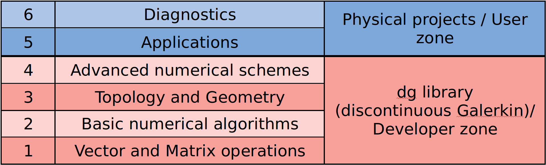
Figure 1: The structure of the project: Feltor is both a numerical library and a scientific software package built on top of that library.

User Zone

A collection of actual simulation projects and diagnostic programs for two- and three-dimensional drift- and gyro-fluid models

6 Diagnostics

These programs are designed to analyse the output from the application programs.

5 Applications

Programs that execute two- and three-dimensional simulations: read in input file(s), simulate, and either write results to disc or directly visualize them on screen. Some examples led to journal publications in the past [63, 32, 43, 62].

Developper Zone

The core dg library of optimized (mostly linear algebra) numerical algorithms and functions centered around discontinuous Galerkin methods on structured grids. Can be used as a standalone library.

4 Advanced algorithms

Numerical schemes that are based on the existence of a geometry and/or a topology. These include for example the discretization of elliptic equations in arbitrary coordinates, multigrid algorithms and a semi-Lagrangian scheme to compute directional derivatives along arbitrary vector fields [33].

3 Topology and Geometry

Here, we introduce data structures and functions that represent the concepts of Topology and Geometry and operations defined on them (for example the discontinuous Galerkin discretization of derivatives [21]). The geometries extension implements a large variety of grids and grid generation algorithms that can be used here [60, 61].

2 Basic algorithms

Algorithms like conjugate gradient (CG) or Runge-Kutta schemes that can be implemented with basic linear algebra functions alone.

1 Vector and Matrix operations

In this "hardware abstraction" level we define the interface for a set of various vector and matrix operations like additions, multiplications, and scalar products. These functions are implemented and optimized on a variety of hardware architectures and serve as building blocks for all higher level algorithms. We study those in Section 4 of this contribution.

2.2 Implications of the code structure

It is possible for several groups to work independently on and with Feltor on the various levels outlined in Fig. 1. Combining the defined building blocks from the lower levels a user can freely construct and explore new numerical algorithms or physical equations. At the same time any improvement or upgrade of the core level routines improves the performance of all application codes using it. Of course, the set of primitive functions also restricts the number of possible numerical algorithms or equations that can be implemented. For example direct solvers are absent in Feltor.

Another advantage is the possibility to test functions and modules separately and independently of each other. We use this feature extensively throughout the development process on all levels outlined in Fig. 1. Specifically, our tests encompass unit tests for low level subroutines, convergence studies of specific numerical algorithms as well as conservation studies of invariants in our physical models.

2.3 Design goals

The implementation of Feltor is the result of an ongoing development process and subject to frequent changes. In the following we thus rather describe our goals and guidelines. These have led to the present state of the code and will likely prevail in the future.

Code readability

Numerical algorithms can be formulated clearly and concisely. In particular, parallelization strategies or optimization details are absent in application codes.

Ease of use

We try to make our interfaces as intuitive and simple as possible. It is possible for C++ beginners to write useful, fast and reliable code with Feltor. This feature is enhanced by an exhaustive documentation and tutorials on our homepage [3].

Fast development

A particular important feature from the user perspective is the possibility to quickly set up or change model equations in a minimum amount of time. We accomplish this feature by providing building blocks at Feltor’s core levels, which can be freely combined or rearranged.

Speed

Feltor provides specialized versions of the performance critical Level 1 functions for various target hardware architectures including for example GPUs and Intel Xeon Phis. Note that writing parallelized code is the default in Feltor. We explore and discuss performance critical issues in Section 4 of this article.

Platform independent

Application code runs unchanged on a large variety of hardware ranging from a desktop environment to mid-sized compute clusters with dedicated accelerator cards. The library adapts to the resources present in the system and chooses correct implementation of functions at compile time. This is possible through a template traits dispatch system in combination with classic C-style macros at Feltor’s core level. We demonstrate this feature explicitly in Section 4 of this article.

Extensibility

The library is open for extensions to future hardware, new numerical algorithms and physical model equations.

Defined scope

Our focus lies on efficient discontinuous Galerkin methods on structured grids and their application to drift- and gyro-fluid equations in two and three dimensions. We outsource any other operation, in particular input/output, to external libraries.

2.4 Getting started

We provide a "Quick start guide" contained in the README file of the dataset [59], which explains how to setup our library on various systems. In Fig. 2, we show a small teaser program to give readers a first impression how code using Feltor looks like. It integrates the function $f(x,y)=\exp(x)\exp(y)$ on the domain $[0,2]\times[0,2]$ using Gauss-Legendre integration.

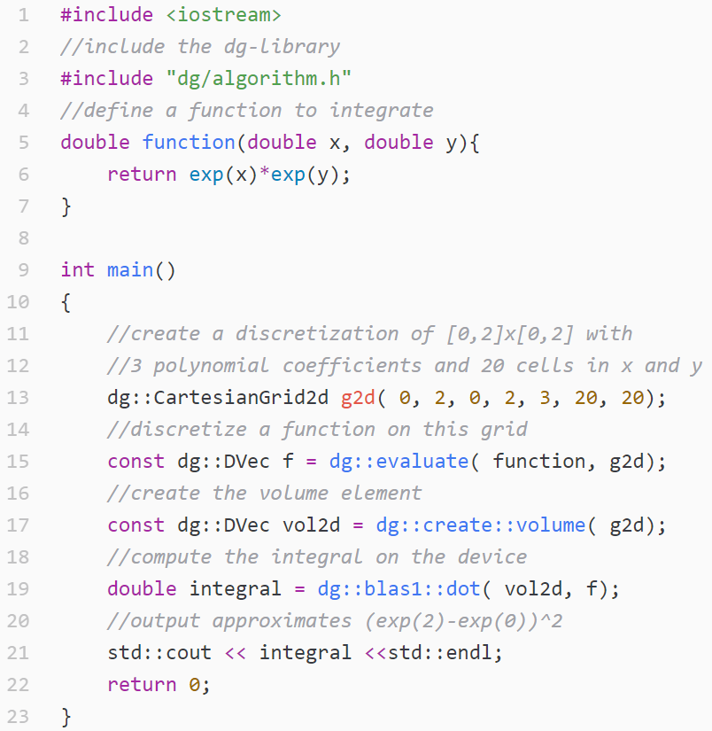
Figure 2: Sample application using Feltor. For details on the function calls see the online documentation.

Depending on how this program is compiled the main computation of the scalar product in line 19 executes either on a GPU or on a shared memory host system. In fact, line 19 is the first example of platform independent code. The dg::blas1::dot function is a template that chooses the implementation based on the vector class it is called with. This means that we could also generate an MPI grid in line 13 and change the dg::DVec to dg::MDVec (an MPI distributed device vector). Then, dg::blas1::dot reroutes to the MPI implementation of the scalar product function. Notice that dg::blas1::dot implements the exact algorithm we discuss in Section 3.

Unfortunately, a more detailed description of the library surpasses the scope of the present article. However, the interested reader will find a helpful tutorial on our webpage[3], which gives a step-by-step introduction to the library and shows and explains many practical code examples. As mentioned earlier, the webpage also contains a more formal documentation of all functions and classes the library provides and pdf files that describe our numerical methods. Hopefully, this will convince the reader that we achieve the design goals outlined previously.

3 Reproducibility in numerical simulations

A paradigmatic model to study drift wave turbulence and zonal flow dynamics in the edge of magnetized fusion plasmas is the Hasegawa-Wakatani (HW) model [28, 56, 29, 50]. Recently, this model has been extended to include large relative density fluctuation amplitudes and steep density gradients within a full-F gyro-fluid approach, thus facilitating studies in the non-Oberbeck-Boussinesq regime [31]. The dimensionless modified full-F HW equations consists of continuity equations for electron particle density $n$, ion gyro-center density $N$ and the polarisation equation

$$\partial_{t}n+\left\{\phi,n\right\} =\alpha\left(\widetilde{\phi}-\widetilde{\ln\left(n\right)}\right),$$ (1a)

$$\partial_{t}N+\left\{\phi-({\nabla}\phi)^{2}/2,N\right\} =0,$$ (1b)

$${\nabla}\cdot\left(N{\nabla}_{\perp}\phi\right) =n-N,$$ (1c)

with electric potential $\phi$, adiabaticity parameter $\alpha$ and Poisson bracket $\{f,g\}:=\partial_{x}f\partial_{y}g-\partial_{y}f\partial_{x}g$. The Reynolds decomposition $f:=\langle f\rangle+\widetilde{f}$ with Reynolds averaged part $\langle{f}\rangle:=L_{y}^{-1}\int_{0}^{L_{y}}dy\hskip 2.84526ptf$ and fluctuating part $\widetilde{f}$ is utilized in the parallel coupling term on the right hand side of Eq. (1a).

The initial (gyro-center) density fields $n(\vec{x},0)=N(\vec{x},0)=n_{G}(x)\left(1+\delta{n}_{0}(\vec{x})\right)$ consist of the reference background density profile $n_{G}:=e^{-\kappa x}$, which is perturbed by a turbulent bath $\delta{n}_{0}(\vec{x})$. Here, $\kappa$ parameterizes the constant background density gradient length. For further details to the model we refer the reader to Reference [31].

We implemented Eqs. 1 in Feltor and now want to test the reproducibility of our parallel simulations. More precisely, we want to test if with the exact same input parameters our executable reproduces the exact same output in subsequent runs. To this end, we fix a typical set of physical and numerical input parameters (contained in the repository [59]) and run our executable twice with the exact same initial condition and parallelization strategy. In Fig. 3 we compare the output of the two runs at each time step. Initially, the relative error $\epsilon_{rel}:=||n_{1}-n_{2}||_{2}/||n_{1}||_{2}$ between the two solutions vanishes. Here, $n_{1}$ and $n_{2}$ is the electron density of the first and second simulation, respectively, and $||f||_{2}$ is the $L_{2}$ norm. As time advances $\epsilon_{rel}$ rapidly increases towards $\mathcal{O}(10^{-1})$.

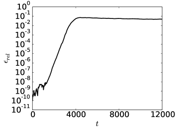
Figure 3: The relative error $\epsilon_{rel}$ as a function of time $t$ is depicted. The relative error $\epsilon_{rel}$ between the naïve runs increases towards $\mathcal{O}(10^{-1})$. Note, that the relative error $\epsilon_{rel}$ is biased by the constant $10^{-10}$.

Although this result is very surprising at first, the possibility for two identical simulation setups to have non-identical results is readily explained. First, let us recall the finite nature (64-, 32-, or 16-bits) of floating-point computations that results in the non-associativity of floating-point operations [23]. For instance, let us denote $\oplus$ as the addition in binary64 floating-point arithmetic, then $(-1\oplus 1)\oplus 2^{-53}\neq-1\oplus(1\oplus 2^{-53})$ since $(-1\oplus 1)\oplus 2^{-53}=2^{-53}$ and $-1\oplus(1\oplus 2^{-53})=0$. Second, in a parallel environment the order of execution between threads is usually arbitrary and can vary between runs. Therefore, subsequent runs of a parallelized executable with identical input may indeed produce various binary outputs. On the other side, if the small round-off errors of machine precision lead to a large error in subsequent simulation times as seen in Fig. 3, then we are apparently faced with an ill-conditioned problem.

Both the fact that executables may produce non-deterministic results and the fact that small derivations may grow exponentially in ill-conditioned problems raise concerns about our ability to reproduce and verify our numerical simulations. In the following we view these concerns from various angles. First, we discuss reproducibility and accuracy from a purely computational and programmatic viewpoint. In Sections 3.1 and 3.2 we present how with the help of so-called long accumulators together with floating-point expansions and error-free transformations we can achieve bitwise reproducibility in our simulations. In the following Section 3.3, we then view the problem from a broader perspective and take computational, numerical and physical considerations into account. We debate the implications of finite machine precision and ill-conditioned problems on the accuracy, convergence, reproducibility, and verification of numerical simulations.

3.1 ExBLAS: Accurate and bitwise reproducible Basic Linear Algebra Subprograms (BLAS)

In this article, we consider the binary64 or double-precision format of the IEEE-754-2008 standard, which requires the basic arithmetic operations $(+,-,\times,/,\sqrt{~{}})$ to be correctly rounded (rounding-to-nearest) [23, 34, 49]. Thanks to the fact that most processors implement this standard, the numerical portability of applications was eased. Due to the finite nature of floating-point computations as well as the non-determinism of parallel executions, we develop an approach to ensure bit-wise reproducibility via ensuring correctly rounded results, whenever possible. The main idea is to keep track of both the result and the errors during the course of computations. To increase the accuracy of floating-point operations, i.e. assure their correct rounding, we rely upon the following two strategies: the first computes the result and recovers the rounding error using so-called error-free transformations (EFT) and stores both result and error in a floating-point expansion (FPE). A FPE is an unevaluated sum of $p$ floating-point numbers whose components are ordered in magnitude with minimal overlap to cover a wide range of exponents. Typically, a FPE relies upon the use of the TwoSum EFT [42] for the addition and the use of the TwoProd EFT for the multiplication [51]. The main advantage of FPEs is that they could be fetched to the registers and reside there during the computation. However, they may not be able to guard every bit of information, which is necessary for correct rounding, for large sums or for floating-point numbers with significant variations in magnitude.

The second strategy projects the finite range of exponents of floating-point numbers into a long vector the so-called long (fixed-point) accumulator. A fixed-point representation stores numbers using an integral part and a fractional part of fixed size, or equivalently a scaled integer. For instance, Kulisch [44] proposed to use a 4288-bit long accumulator for the exact dot product of two vectors composed of binary64 numbers; however, such a large long accumulator is designed to cover all the severe cases without overflows in its highest digit. By preserving every bit of information, the long accumulator guarantees to compute the exact result of a large amount of floating-point numbers of arbitrary magnitude. However, when comparing to FPE, the long accumulator has a large memory footprint and requires roughly two times more operations to be performed.

With the aim to derive fast, accurate, and reproducible Basic Linear Algebra Subprograms (BLAS), we construct a multi-level approach for these operations that is tailored for various modern architectures with their complex multi-level memory structures. On one side, we want this approach to be fast to ensure similar performance compared to the non-deterministic parallel versions. On the other side, we want to preserve every bit of information before the final rounding to the desired format to assure correct-rounding and, therefore, reproducibility. To accomplish our goal, we merge together FPE and long accumulators, tune them, and efficiently implement them on various architectures, including conventional CPUs, Nvidia and AMD GPUs, and Intel Xeon Phi co-processors (for details we refer to Reference [13]).

We begin with the parallel reduction, which is at the core of many BLAS routines. We build its scalable, accurate, and reproducible version using FPEs with the TwoSum EFT [42] and long accumulators. In practice, the latter is so rarely invoked that only little overhead (less than $8$ %) results on summing large vectors. The dot product of two vectors is another crucial fundamental BLAS operation. The exdot (exact stands for accurate and reproducible) algorithm is based on the previous exsum algorithm and the TwoProd EFT [51]: we accumulate both the result and the error to FPEs and reduce these FPEs and long accumulators on various levels as in exsum. These and other routines – such as matrix-vector product (exgemv), triangular solve (extrsv), and matrix-matrix multiplication (exgemm) – are distributed as the Exact BLAS (ExBLAS) library [35, 36]. Thanks to the modular and hierarchical structure of linear algebra algorithms, higher level operations – such as matrix factorizations – can be entirely built on top of the fundamental kernels as those in the BLAS library. In ExBLAS, we follow this principal to construct reproducible LU factorizations with partial pivoting.

3.2 Reproducibility in Feltor

As outlined in Section 2 Feltor builds its algorithms on basic primitive functions, which partly overlap with the BLAS library. Please find the exact list of functions in the documentation. Our basic assumption is that, if these elementary functions are reproducible, then all algorithms and simulations implemented with them are reproducible. This assumption follows our theoretical and practical studies [37] of the unblocked LU factorization with partial pivoting, which underneath is entirely build upon the BLAS routines. The first step to realize our goal incorporates the correctly rounded and reproducible parallel reduction from the ExBLAS library into Feltor. In this way, we can provide the accurate and reproducible dot product $\sum_{i}x_{i}y_{i}$. Note that we also provide a function computing the weighted sum $\sum_{i}x_{i}w_{i}y_{i}$, where $w$ represents for example the volume form of our coordinate system. This is important in numerical computations of the scalar product $\int f_{1}f_{2}\sqrt{g}\text{d}V$ with functions $f_{1}$, $f_{2}$ and volume element $\sqrt{g}$.

In the second step we make the trivially parallel vector operations like $y\leftarrow\alpha x+\beta y$ reproducible. Unfortunately, the use of FPEs or long accumulators for these very small summations introduce too much overhead to be practical. Hence, our idea is to just fix the type and order of execution of floating point operations. The results should then be identical for all compilers and platforms that follow the IEEE-754-2008 standard. The problem with this is that for performance reasons, the C++ language standard allows compilers to change the execution order of a given line of code. It even allows merging multiplications and summations with fused multiply add (FMA) instructions. This computes a*x+b in a single instruction with only a single rounding operation at the end. Let us consider the ’naive’ implementation y=a*x+b*y. A compiler might translate this to two multiplications t1=a*x and t2=b*y and a subsequent summation y=t1+t2; it might generate a single multiplication t=b*y with a subsequent FMA y=fma(a,x,t), which gives a slightly different result; or it may even compute t=a*x first and then use the FMA y=fma(b,y,t).

Our approach to solve this issue is to explicitly instruct the compiler to use FMAs together with relevant compiler flags to prevent the use of value changing optimization techniques (for example -fp-model precise for the Intel icc compiler). The former is possible through the std::fma instruction added to the C++ -11 language standard. With this combination we avoid non-determinism in the order of operations, reduce the number of rounding errors from three to two, and, therefore, achieve bitwise reproducibility for this operations and even for matrix-vector multiplications $y\leftarrow\alpha Mx+\beta y$. Again, we do not use long accumulators for the summation but only fix the order of execution. However, we need to take special care in our MPI implementation. The computation of boundary points can begin only after all values from other processes were communicated.

The third step towards reproducibility in Feltor is to make the initialization of vectors reproducible. Here, the main problem lies in the use of transcendental functions like $e^{x}$, $\sin(x)$ or $\cos(x)$. The algorithms for computing these functions differ by compiler and the results subsequently differ if not correctly rounded. A practical and portable solution to this problem is an open issue in Feltor.

All in all, Feltor yields reproducible results up to the compiler and the hardware’s capability to compute FMAs. This means that we can reproduce simulation results bit for bit, independently of parallelization, as long as we use the same compiler and the CPU is capable of computing FMAs.

3.3 Bitwise reproducibility, accuracy, convergence and verification

We improved Feltor with the reproducible BLAS Level-1 subroutines and can now re-simulate Eqs. 1 and indeed obtain bitwise identical results after each run. Please consult the dataset [58] introduced in Section 4 for details on the exact compiler flags and hardware that we use for our simulations. We show our solution in Fig. 4 where we compare the radial zonal flow structure to the previous implementation. Here, the radial zonal flow structure of the naïve implementation deviates while the zonal flow structures are identical in the new (reproducible) implementation.

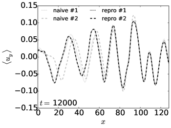
Figure 4: The radial zonal flow signature is shown. The deviation of zonal flow structure of two naïve runs with identical initial conditions is clearly visible. As opposed to this the zonal flow structure of the bitwise reproducible runs are identical.

Let us summarize the implications of what we have achieved and know up to this point.

Bitwise reproducibility

We have the possibility to reproduce parallel simulation results bit-to-bit. This is particularly advantageous from a programmatic point of view since alterations in the implementation or future adaptions to other parallel hardware can be rigorously checked and tested. Moreover, independent outside groups and ourselves gain the possibility to re-simulate and confirm the results. This is especially important since we usually refrain from publishing output files due to their impractically large size. Now, we have the possibility to publish the code together with input files and can expect to exactly reproduce presented results [59].

Accuracy

It is important to mention that we not only achieved bitwise reproducibility but also increased the accuracy of our implementation, mainly in the scalar product. The latter is for example important in a conjugate gradient method. The problem with the previous naïve summation was the unfavourable cancellation of digits when adding small values to a large sum. Even in a tree summation algorithm the error grows with the size of the array with $\sqrt{a}$ with $a$ being the array size. This effectively reduces the machine precision, which is a particular concern for large scale single precision computations. It is expected that the next generation of supercomputers – such as Exascale systems delivering $10^{18}$ floating-point operations per second – will be composed of heterogeneous resources like CPUs and accelerators. Obtaining peak performance on these systems will, in all likelihood, require the use of single or mixed-precision simulations [7, 8, 11, 17].

Condition

If we evolve the physical model Eqs. 1 over long periods of time, even small (physical) perturbations in the initial state can be amplified by many orders of magnitude. This is a fundamental property of the physical system under consideration. Consequently, this behaviour is also reflected in the numerically discretized system of equations. Recall that (numerical) perturbations are always present in this system. For example, even if the initial state is given by an analytical function its numerical representation is already inexact due to either the discretization error or the finite precision of floating point arithmetics. These (numerical) perturbations then grow over time just as their physical counterparts do.

In conclusion, we have to accept that even with the increased accuracy and reproducibility of our implementation the error in our numerical solution is large after a sufficiently long simulation time. This is because any error stemming either from the numerical discretization or the finite machine precision will be amplified by the system. In particular this means that we cannot obtain convergence of our simulation. Even with infinite machine precision we would need a prohibitively fine grid to find the exact solution. On the other side, the error in a single time-step or small enough time span may still be acceptable and converge with the expected order. For example in Fig. 3 the error from machine precision is still small for times below $t=2000$ say, such that a convergence study is possible in this regime. In this context, we can also expect that as long as we can maintain the machine precision in our implementation (especially for the dot product, as discussed above) using single precision gives the same physical results as does double precision. In memory bandwidth bound problems this can potentially lead to a factor two gain in performance.

Furthermore, we have to reject the notion that our bitwise reproducible solution is any more physically or numerically reasonable than the previous solution, even if the accuracy of elemental operations was increased. We only select one specific solution out of a larger class of solutions equivalent within the limits of the accuracy of the numerical discretization and the machine precision. In fact, we can also physically expect a larger class of end states that are equivalent within small (thermal) fluctuations that are present in the turbulent system described by Eqs. 1.

All of these points raise the question: how and in what sense can we then consider simulation results to be "correct"? The answer to this question depends on what the goal of the simulation effort is. A first step is to identify quantities that are of physical interest. This can for example be the zonal flow structure in Fig. 4 or turbulent spectra. Convergence can then be studied directly in terms of the physical quantities that we are interested in. In many situations, these quantities show convergence even though pointwise convergence of the numerical solution can not be achieved (see, for example, [20]). In addition, we recommend checking that the quantities of interest are insensitive to very small perturbations. This can be done by performing simulations of an ensemble of slightly perturbed initial values. If the quantities of interest have similar values for the entire ensemble, confidence in the corresponding numerical results is increased.

Finally, invariants of the physical model can be used as a consistency check of the numerical method and the corresponding implementation. Also, they help to restrict the range of possible solutions to the system. This, on one hand, means that we should favour physical models that do provide invariants and numerical methods that conserve these invariants. Conservative numerical methods can (often) give us a good physical picture even though the $L^{\infty}$ error is large. On the other hand, it is difficult to guarantee correct (physical) behaviour from symmetries of a system alone. For example energy conservation is in general not enough to guarantee physical solutions. As exemplified by the integration of the solar system in [25, Chap. 1], a numerical integrator may be locally converged and conserve energy and still produce a strikingly wrong (both qualitative and quantitative) result after a long time. Ultimately, we will have to accept that if the physical interest is the exact result (for example the precise velocity fluctuations in a turbulence simulation), the possible simulation time span is largely reduced depending on the condition of the system. We note again that this is not an algorithmic or implementation problem. It is rather a consequence of the physical properties of the system that we investigate.

4 Performance and runtime prediction

In this Section we present a performance study of the Feltor library. This study includes a second dataset [58] to this article, which provides the complete raw data in csv format as well as the ipython notebooks used for the data analysis and plot generation. The interested reader is invited to inspect these notebooks in parallel to reading this section for additional information and details.

We begin this section with a discussion of important performance optimization techniques for memory bandwidth bound algorithms 4.1. We then shortly describe the hardware, the configuration and the program that we used to generate the performance data 4.2. Having measured and discussed the performance of Feltor’s building blocks in Section 4.3 we suggest a performance model that predicts the runtime of any constructed algorithm in Section 4.4. We discuss strong and weak scaling in Section 4.5 and conclude with a critical discussion in Section 4.6.

4.1 Optimization techniques for low-level Feltor routines

As mentioned in Section 2, the Level 1 algorithms implemented in Feltor include basic linear algebra routines that build the dg library code. Besides trivially parallel vector operations like addition or pointwise multiplication, we implemented the scalar product with long accumulators (Section 3) and a sparse matrix-vector multiplication. Optimizing these operations is a key task in order to increase the overall performance of any higher level algorithm or application using Feltor.

Note, that we devised our own sparse block matrix format, which specifically saves storage on redundant blocks and thus potentially fits into small and fast memory caches of the target architecture. It is used for the computation of the simple discontinuous Galerkin derivative in $x$ and $y$ on product spaces (see Reference [21] for more details). Many algorithms, including the Arakawa scheme [21] or the discretization of elliptic problems [12, 6], build on those derivatives. An optimization of the corresponding matrix-vector product will thus greatly contribute to reducing their execution times.

In general, vector additions, sparse-matrix-vector multiplications and scalar products require a similar amount of memory and arithmetic operations. This means that on all modern hardware architectures these routines are memory bound. However, this conclusion assumes an efficient implementation. In particular, it assumes that our code is able to exploit the parallelism present on these architectures in order to saturate the available bandwidth. In addition, to achieve optimal performance, memory has to be read in a sequential (coalesced) manner. This is especially true for the Intel Xeon Phi "Knights Landing" accelerator card (KNL) and GPUs.

The easiest option to optimize a code for a new architecture such as KNL is to recompile it with the proper flags (discussed for KNL further below) and thus get an instantaneous benefit. However, achieving a full and efficient use of a new architecture requires an analysis using available profiling tools and an optimization effort, which is reflected normally in code modifications.

The strategy to optimize a code for a given architecture involves different levels, beginning from the core level to the outer levels of the hardware, since all the optimizations introduced in any level automatically benefits its upper levels.

Most modern processors have so-called vector units that allow it to execute a single instruction on multiple data (SIMD) per cycle. For example, each KNL core has two 512-bit vector units that enable it to compute 16 double precision operations concurrently. The usage of these SIMD (or vector) instructions in a loop is called vectorization.

Most compilers may vectorize loop structures automatically to take advantage of vector units if they are called with the proper options. For the KNL, the intel compiler provides -xMIC-AVX512 to enable AVX-512 vector instruction set [39], -fma to generate fused multiply-add (FMA) instructions and -align to use aligned load or store vector instructions.

However, the vectorization report generated by the compiler typically shows that not all loops can be vectorized. The compiler only vectorizes when it considers this process a) safe and b) improves the performance. This means that in order to achieve a good performance sometimes we have to help the compiler to vectorize loops initially discarded by it. For example, when the compiler believes that two pointers in a loop may reference a common memory region implying likely data dependencies among iterations the compiler refrains from vectorization. This situation can be solved using the keyword restrict for a pointer argument in a C/ C++ function, which indicates that the pointer argument provides exclusive access to the memory referenced in the function and no other pointer can access it.

Another example is when the compiler does not vectorize a loop because an efficiency heuristics predicts that this vectorization will lead to a worsening of the performance, such as the presence of many unaligned data accesses. This time it can be solved introducing the OpenMP-4 extension #pragma omp simd, which explicitly tells the compiler that it is safe to use SIMD instructions. As an example of its application, the following loop in the code reduced the total number of executed instructions by 86% thanks to enabling SIMD instructions.

#pragma omp parallel for simd
for (unsigned u = 0; u < size; ++u)
  y_ptr[u] = alpha * x_ptr[u] + beta * y_ptr[u];

In general we observe that vectorization significantly improves the performance of the scalar product with long accumulators, our sparse matrix-vector multiplication and to a lesser extent also the vector additions.

Continuing with the higher hardware level, a KNL node contains 68 cores, so a good thread scalability is mandatory to take advantage of them. In the case of the sparse-matrix vector multiplication, the previous code contained three consecutive OpenMP parallel regions that were merged into one to give all threads more work reducing idle time and overhead costs, such as thread management and synchronization. Besides, KNL offers hyperthreading, which means that each core supports up to $4$ threads, leading to the possibility of using up to $272$ threads per KNL node. As hyperthreading may improve performance when memory access latency limits the execution, some performed experiments suggested to run at least $2$ threads per core in order to increase the full core usage and so improve performance.

Finally, we observe that making the number of polynomial coefficients a compile time constant (a template parameter) resulted in another significant improvement of runtime in the matrix-vector multiplication. The coefficient fixes the size of the blocks in the sparse matrix format and thus the size of the tight inner loops of the routine is known at compile time which allows the compiler to generate more efficient code. This is a common technique that has been utilized in a range of C++ implementations (see, for example, [24, 38, 19, 18]).

Note that all the optimizations that have been performed for the KNL have a positive effect on the regular CPU performance as well. On GPUs we observe similar performance improvements when we add the restrict keyword to pointer arguments in the corresponding kernels and use template arguments as well. We can avoid warp divergence since if-clauses are absent in our implementations.

4.2 Configuration

We use the program feltor/inc/dg/cluster_mpib.cu that is contained in [59], together with suitable submit scripts in [58], for generating the performance data. Essentially, we gather the average run times of a variety of primitive functions, the Arakawa algorithm and a conjugate gradient iteration. Let us note here that the results from different architectures are bitwise identical as long as we only compare results from the same compiler (see Section 3). We vary problem sizes and number of compute nodes on a selection of representative hardware architectures, which includes a current consumer grade desktop CPU and GPU, as well as dedicated high performance compute hardware from Intel and Nvidia. Please find a short description of the configuration in Table 1 and more details in the dataset [58]. We refer to the documentation of the dg::Timer class in [59] for details of how we measure the time on the various architectures involved.

	device description	single-node configuration
i5	Intel Core i5-6600 @ 3.30GHz (2x 8GB DDR4, 4 cores)	1 MPI task x 4 OpenMP threads (1 per core)
skl	2x Intel Xeon 8160 (Skylake) at 2.10 GHz (12x 16GB DDR4, 2x 24 cores)	2 MPI tasks (1 per socket) x 24 OpenMP threads (1 per core)
knl	Intel Xeon Phi 7250 (Knights Landing) at 1.40 GHz (16GB MCDRAM, 68 cores)	1 MPI task x 136 OpenMP hyperthreads (2 per core)
gtx1060	Nvidia GeForce GTX 1060 (6GB global memory)	1 MPI task per GPU
p100	Nvidia Tesla P100-PCIe (16GB global memory)	1 MPI task per GPU
v100	Nvidia Tesla V100-PCIe (16GB global memory)	1 MPI task per GPU

Table 1: Description of the tested compute nodes: device description and total RAM size as well as the corresponding distribution of MPI tasks and OpenMP threads/GPU contexts. The configuration of multiple nodes scales the number of MPI tasks; for example $4$ skl nodes involve $8$ MPI tasks each spawning $24$ OpenMP threads running on $192$ physical cores.

4.3 Performance measurements

From the measured runtime $t$ and the array size $S$ we compute the memory bandwidth $b$ of an algorithm or function

$$b=\frac{mS}{t}$$ (2)

where $m$ is the number of memory loads and stores. We follow the STREAM conventions in counting memory operations, which means that we separately count each read and each write of a memory location. For example the vector addition axpby, which computes the operation $y\leftarrow\alpha x+\beta y$, counts as $m=3$ times the vector size since we have to read both $x$ and $y$ and then write into $y$. The dot product $x\cdot y$ counts as $m=2$ times the vector size.

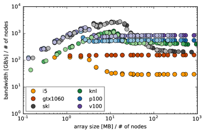
(a) axpby

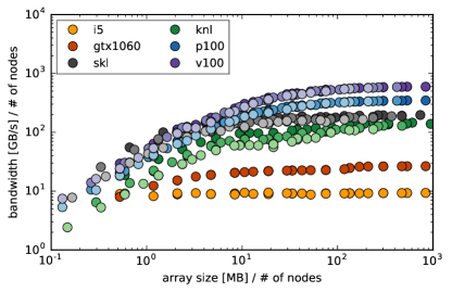
(b) dot

Figure 5: Single node memory bandwidth plot of the trivially parallel vector addition (a) and the exact dot product (b) on various hardware architectures on one node (full saturation color), on two nodes (medium saturation) and on four nodes (low saturation). We normalize to the number of nodes, such that the single node performance becomes visible.

In Fig. 5 we plot the average bandwidth $b$ for various hardware architectures and problem sizes $S$. We normalize the plot to the number of nodes $n$, $b/n$ and $S/n$, such that each point represents the performance of a single node.

First, we note that in both, Fig. 5a and Fig. 5b the lightly colored points from multi-node runs lie almost exactly on top of their single-node counterparts. This is especially true for the P100 and V100 GPUs and the Skylake nodes but is not so well fulfilled for the Xeon Phi. The feature indicates a high weak scaling efficiency of both axpby and dot, which means that the achievable bandwidth of a given node is given solely by the problem size on the node itself.

Next, we note that in Fig. 5a the bandwidth for small to medium sized problems ($1$MB $<S/n<10$MB) is significantly higher than for large problems ($S/n>100$MB) for all architectures (note that the lowest sized point of the ’gtx1060’ is hidden beneath a ’skl’ point). This is especially pronounced for the Skylake architecture. We explain this by the cache level hierarchy. The problem fits entirely into the cache such that its higher speed becomes visible. In fact, the peaks roughly coincide with the relevant cache sizes (see [58] for exact cache sizes). This feature is absent in Fig. 5b, which is most likely due to the high number of 64-bit operations per memory load in the long accumulator scalar product.

For the multi-node architectures we identify a linear regime for small array sizes ($S/n<2$MB) in both Fig. 5a and 5b. Here, the bandwidth increases linearly with the array size, which indicates a size-independent runtime $T_{\text{lat}}$, called the latency. Note that the multi-node results in Fig. 5b indicate an increasing latency for multiple nodes. We explain this by the necessary global communication between nodes due to the reduction, which is absent in the axpby algorithm. On the other hand, for large array sizes ($S/n>100$MB) we identify a regime with constant bandwidth $B$ in both Fig. 5a and 5b independent of node number.

	peak	axpby			dot
	bandwidth [GB/s]	bandwidth [GB/s]	$T_{lat}(1)$ [$\mu$s]	$T_{lat}(4)$ [$\mu$s]	bandwidth [GB/s]	$T_{lat}(1)$ [$\mu$s]	$T_{lat}(4)$ [$\mu$s]
i5	34	30 $\pm$ 01	00 $\pm$ 02	n/a	10 $\pm$ 01	05 $\pm$ 01	n/a
gtx1060	192	158 $\pm$ 01	00 $\pm$ 01	n/a	27 $\pm$ 01	93 $\pm$ 09	n/a
skl	256	207 $\pm$ 06	00 $\pm$ 01	00 $\pm$ 01	193 $\pm$ 19	18 $\pm$ 03	38 $\pm$ 05
knl	>400	394 $\pm$ 23	06 $\pm$ 01	10 $\pm$ 01	142 $\pm$ 07	55 $\pm$ 02	120 $\pm$ 06
p100	732	554 $\pm$ 01	01 $\pm$ 01	03 $\pm$ 01	347 $\pm$ 02	49 $\pm$ 01	49 $\pm$ 01
v100	898	849 $\pm$ 01	02 $\pm$ 01	03 $\pm$ 01	594 $\pm$ 03	34 $\pm$ 02	35 $\pm$ 01

Table 2: Measured single node bandwidth and latency on a single node and four nodes of apxby and dot. The peak bandwidth is the theoretical RAM bandwidth according to the vendors. The exact peak bandwidth of the MCDRAM on knl was not disclosed to us.

We determine $B$ by taking the average bandwidth of the largest array sizes and estimate an error with the standard deviation. This is in general a very robust method and yields small errors in our experience. The correct determination of the latency $T_{\text{lat}}$ is more involved with the available data. We differentiate between single-node and multi-node latency. As a first approximation we simply identify the minimum average runtime with $T_{\text{lat}}$ and again use the standard deviation as an error estimate. If we now assume that the runtime is given by

$$t=T_{\text{lat}}(n)+\frac{mS}{nB},$$ (3)

then we can correct the minimum runtime $t_{\text{min}}$ by $-mS/B$ with the previously measured $B$ to obtain a better approximation to $T_{\text{lat}}$. However, with the exception of the Knights landing architecture the single-node latencies for axpby are so small that the values become negative. In this case we replace the value by $0$. In Table 2 we give numerical values of the bandwidths together with the latencies as well as the peak bandwidth according to the vendors. Within the error the axpby latencies can be neglected altogether except for the Knights Landing architecture.

We note that the GPUs and the Xeon Phi have the highest latencies in the dot algorithm. The high GPU latency is the result of the slow PCIe lanes since the result has to be sent back to the host CPU, which entails communication. As already evident in Figure 5b the latencies on multiple nodes significantly increase for the Xeon Phi and the Skylake architectures. This indicates a long latency of the internode connection. For the P100 and V100 GPUs the latency seems to be dominated by the communication between GPU and host CPU.

Finally, we note that all architectures reach only $75\%$ (p100) to $95\%$ (v100) of their theoretical peak bandwidth in the axpby function. This is in line with previous observations of the STREAM benchmark [15]. We do not know of any practical method to overcome this performance degradation programmatically and consider the measured bandwidth $B^{\texttt{axpby}}$ as the maximum bandwidth any memory bound algorithm can achieve on the given architecture. In this sense, the Skylake architecture reaches almost $100\%$ efficiency for the dot algorithm, followed by the Tesla cards P100 and V100. The GTX 1060 has the lowest efficiency, which is most likely due to the drastic reduction of double precision performance on the gaming GPU (a factor $32$ compared to single precision), which is absent in the Tesla GPUs.

	B(P=2) [GB/s]	B(P=3) [GB/s]	B(P=4) [GB/s]	B(P=5) [GB/s]	$T_{lat}(1)$ [$\mu$s]	$T_{lat}(4)$ [$\mu$s]
i5	28 $\pm$ 03	30 $\pm$ 03	26 $\pm$ 02	22 $\pm$ 02	00 $\pm$ 02	n/a
gtx1060	131 $\pm$ 01	112 $\pm$ 02	84 $\pm$ 14	70 $\pm$ 18	00 $\pm$ 01	n/a
skl	182 $\pm$ 36	162 $\pm$ 13	119 $\pm$ 19	111 $\pm$ 09	23 $\pm$ 03	29 $\pm$ 03
knl	240 $\pm$ 18	173 $\pm$ 27	127 $\pm$ 19	102 $\pm$ 15	10 $\pm$ 01	53 $\pm$ 04
p100	288 $\pm$ 03	238 $\pm$ 04	201 $\pm$ 02	166 $\pm$ 15	02 $\pm$ 01	64 $\pm$ 01
v100	802 $\pm$ 17	713 $\pm$ 20	650 $\pm$ 16	536 $\pm$ 49	04 $\pm$ 01	67 $\pm$ 02

Table 3: Single node bandwidth of a DG matrix-vector multiplication for various polynomial coefficients $P$. Latencies on a single node/card and four nodes/cards.

For the matrix-vector product we perform the same analysis and show the results In Table 3. There, we present the average bandwidth between a DG derivative in the x-direction and the y-direction, which we call dxdy. Due to our efficient format the matrix itself does not contribute to the memory loads and stores. We count two loads and one store for the $y\leftarrow\alpha Mx+\beta y$ operation ($m=3$). However, we do differentiate between various polynomial orders, which determines the stencil of the operation. A higher polynomial order increases the registry pressure and thus decrease the efficiency of the implementation. The latency should not be influenced by the polynomial order and we provide the latencies for the $P=2$ case. We observe the highest latencies for the multi-node configurations. Here, the algorithm involves communication between neighboring processes. This is particularly unfavourable for the GPUs since these have to communicate via the host CPU across the PCIe lanes.

Concerning the single node bandwidths $B$ we overall observe the highest values for the Tesla GPUs. It is noteworthy that the GTX 1060 has a very low latency and reaches almost $70\%$ of the bandwidth of the much more expensive Skylake and Xeon Phi nodes.

4.4 Performance prediction model

Any one of the primitive subroutines in Level $1$ in Feltor falls into one of the categories ’trivially parallel’ (axpby), ’nearest neighbor communication’ (dxdy) and ’global communication’ (dot). We specifically measured the bandwidths and latencies of the three operations axpby, dxdy and dot in Tables 2 and 3. For the following discussion we assume that these values accurately represent the bandwidths and latencies of the whole respective class of functions. In fact, we use these values to predict the runtime of any algorithm that is implemented in terms of Level $1$ subroutines. For a given architecture and node number $n$ we predict a runtime $t$ depending on the array size $S$ and the number of polynomial coefficients $P$

$$t(P,S,n) =\sum_{q}\sum_{i=0}^{N_{q}-1}t_{i}^{q}(P,S,n)=\sum_{q}\left[N_{q}T^{q}_{\text{lat}}(n)+\frac{M^{q}S}{nB^{q}(P)}\right]$$

$$=:N\left[T_{\text{lat}}(n)+\frac{M}{N}\frac{S}{nB(P)}\right]$$ (4)

$$T_{\text{lat}}(n) :=\frac{1}{N}\sum_{q}N_{q}T^{q}_{\text{lat}}(n)$$ (5)

$$\frac{1}{B(P)} :=\frac{1}{M}\sum_{q}\frac{M^{q}}{B^{q}(P)}$$ (6)

with the function type $q\in(\texttt{axpby,dot,dxdy})$, $i$ iterates over all occurrences of function type $q$, $N_{q}$ is the total number of occurrences of all functions of type $q$, $M^{q}$ is the total number of memory loads and stores among functions of type $q$, $B^{q}(P)$ is the single node memory bandwidth of function type $q$ and $T^{q}_{\text{lat}}(n)$ is the latency depending on the number of nodes used. In Eqs. (5) and (6) we defined the average latency and weighted average single node bandwidth, where $N:=\sum_{q}N_{q}$ and $M:=\sum_{q}M^{q}$. The values for $B^{q}(P)$ and $T^{q}_{\text{lat}}(n)$ are in Table 2 and 3. We present an average over a conjugate gradient iteration and the Arakawa algorithm in Table 4. These two algorithms represent a typical mixture of primitive functions used in a Feltor simulation project. In fact, we get a first approximation of the runtime of any algorithm by counting the total number of function calls $N$ and using Eq. (4), Table 4 and $M/N\approx 3.3$.

	B(P=2) [GB/s]	B(P=3) [GB/s]	B(P=4) [GB/s]	B(P=5) [GB/s]	$T_{lat}(1)$ [$\mu$s]	$T_{lat}(4)$ [$\mu$s]
i5	26 $\pm$ 02	27 $\pm$ 02	26 $\pm$ 01	23 $\pm$ 02	01 $\pm$ 01	n/a
gtx1060	116 $\pm$ 01	108 $\pm$ 01	94 $\pm$ 09	85 $\pm$ 12	09 $\pm$ 01	n/a
skl	194 $\pm$ 20	183 $\pm$ 09	153 $\pm$ 15	147 $\pm$ 07	14 $\pm$ 02	19 $\pm$ 02
knl	281 $\pm$ 13	232 $\pm$ 24	188 $\pm$ 20	160 $\pm$ 18	13 $\pm$ 01	42 $\pm$ 02
p100	377 $\pm$ 02	333 $\pm$ 04	297 $\pm$ 02	259 $\pm$ 17	06 $\pm$ 01	39 $\pm$ 01
v100	808 $\pm$ 09	763 $\pm$ 11	727 $\pm$ 10	653 $\pm$ 35	06 $\pm$ 01	39 $\pm$ 01

Table 4: Average single node bandwidths $B$ for various polynomial coefficients $P$ as well as average single-node and multi-node latencies according to Eq. (4). We use Table 2 and 3, $(N^{\texttt{axpby}},N^{\texttt{dot}},N^{\texttt{dxdy}})=(9,2,12)$ and $(M^{\texttt{axpby}},M^{\texttt{dot}},M^{\texttt{dxdy}})=(36,4,36)$, $N=23$, $M=76$ and a ratio of $M/N=3.30$. This corresponds to the average between a conjugate gradient iteration and the Arakawa algorithm.

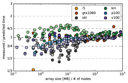
(a) arakawa

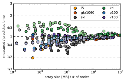
(b) cg

Figure 6: Comparison of predicted runtime Eq. (4) to measured time for the Arakawa algorithm (a) and a single conjugate gradient (cg) iteration (b). The plot highlights the deviation from the predicted time. Points below $1$ mean faster execution than predicted.

In Fig. 6 we compare the result of the prediction in Eq. (4) with the measured runtime for the arakawa algorithm and one cg iteration. The plots depict the relative error of the prediction. If a point lies below $1$, the execution was faster than predicted. Especially for large array sizes $S/n>30$MB our prediction is accurate for all architectures. We note in both Fig. 6a and Fig. 6b that the measured runtime for the Xeon Phi card on multiple nodes for sizes $S/n<20$MB is systematically overestimated. On the other side the Skylake architecture and the Intel i5 CPU for array sizes $S/n<30$MB run up to a factor $2$ faster than predicted. We explain this by the very fast execution of the trivially parallel part of the algorithms in the fast cache as is evident in Fig. 5a. This effect is not included in our parallel model. On the other hand, the measured run times $T^{\text{meas}}$ for the Tesla GPUs and our desktop system are remarkably well predicted by our model and with only few exceptions lie within an interval $(3/4)T^{\text{pred}}<T^{\text{meas}}<(4/3)T^{\text{pred}}$, with $T^{\text{pred}}$ given by Eq. 4.

4.5 Strong and weak scaling

Equation (4) enables us to discuss the strong and weak scaling of an arbitrary algorithm. The strong scaling of a problem with total array size $S$, polynomial coefficients $P$ and number of nodes $n$ is defined as

$$\varepsilon(P,S,n):=\frac{t(P,S,1)}{nt(P,S,n)}=\frac{T_{\text{lat}}(1)+(M/N)(S/B(P))}{nT_{\text{lat}}(n)+(M/N)(S/B(P))}$$ (7)

The weak scaling efficiency relates run times with equal array size per node $s=S/n$ as

$$\gamma(P,s,n):=\frac{t(P,s,1)}{t(P,ns,n)}=\frac{T_{\text{lat}}(1)+(M/N)(s/B(P))}{T_{\text{lat}}(n)+(M/N)(s/B(P))}$$ (8)

We immediately see that the efficiency $\varepsilon$ tends to $0$ for large number of nodes $n$, while the explicit $n$ dependency in $\gamma$ vanishes. The only remaining dependence on $n$ is in the latency $T_{\text{lat}}(n)$. We argue that the dependence on $n$ should vanish in the latencies for axpby, since there is no communication at all. For the dxdy algorithm the latencies should also become independent of $n$ for large $n$ since communication happens only between nearest neighbors. Only for the dot product the latency should increase with $n$ due to the global communication.

Both the strong and the weak scaling tend to unity if $s=S/n\gg(N/M)T_{\text{lat}}(n)B(P)$. The value of the product

$$(S/n)_{\text{min}}\approx 0.3T_{\text{lat}}(n)B(P)$$ (9)

is the minimum size per node for a Feltor simulation with a scaling efficiency of at least $50\%$ (both $\varepsilon$ and $\gamma$ are $>0.5$ for $S/n>(S/n)_{\text{min}}$). For the values presented in Table 4 the minimum array size per node typically lies between $1$ and $10$MB.

Note that for fixed latencies the scaling efficiencies $\varepsilon$ and $\gamma$ are low if the bandwidth is high and vice versa high if the bandwidth is low. This is ironical since the runtime $t$ is low if the bandwidth is high as evident in Eq. (4). A high scaling efficiency is thus not necessarily an indicator for an efficient implementation just as a low scaling efficiency not necessarily points to inefficient code.

4.6 Discussion

From Eq. (4) it is clear that the runtime $t$ is low if the average latency $T_{\text{lat}}$ is low and the bandwidth $B$ is high. On the other side, performance can also be gained by reducing the number of function calls $N$, or the number of memory operations $M$. Apparently, the fastest possible implementation is to implement the whole algorithm in a single function, with $N=1$ and a minimum number of memory operations $M_{\text{min}}$. For example, our current arakawa implementation has $M=34$ and $N=9$, which compares unfavourably to a possible $N_{\text{min}}=1$ and $M_{\text{min}}=4$. The drawback of implementing and optimizing every algorithm or equation separately is the increased maintenance and performance tuning cost. Furthermore, this approach would not be easily extensible or modifiable and violates our design goals presented in Section 2. Still, we estimate the performance we loose due to the Feltor design between a factor $2$ and $5$ depending on the algorithm at hand. In an effort to mitigate the problem we introduced new primitive functions with increased workload, for example the vector operation $z\leftarrow\alpha x_{1}y_{1}+\beta x_{2}y_{2}+\gamma z$, where $x_{1}y_{1}$ is a point-wise multiplication. We currently also explore template parameter packs in the C++ -11 standard as a promising candidate to increase the workload of Level 1 functions in Feltor.

5 Discussion and Conclusion

With Table 4 and Eq. 4 in Section 4 we have a powerful tool to judge the performance of various hardware architectures available to us. We are able to estimate the runtime of a Feltor simulation for given problem size, hardware and node count. Furthermore, with Eq. (9) we have an easy to use estimate of the minimum array size per compute node for an acceptable scaling efficiency. From a user perspective this estimate and the possibility to predict runtimes are certainly valuable features since available resources can be used more effectively and the performance of future hardware can be estimated from its theoretical bandwidth.

Let us here discuss performance also in the light of the simulations we eventually want to carry out. In fact, an increase/decrease in performance of the implementation may lead to an only marginal improvement/deterioration of the numerical simulations itself. Consider for example a three dimensional problem and an available runtime $T$ (set by cluster policies, allocated resources or simply personal preferences). Accounting for the reduced/increased time step due to the CFL condition a factor $2$ increase/decrease in performance leads to only a factor $2^{1/4}\approx 1.19$ increase/decrease in the number of grid points per dimension. This justifies our design goals laid out in Section 2. We do strife for performance but when faced with possible trade-off scenarios we put equal value on other goals as well.

Of course, the choice of the physical model and the numerical methods employed ultimately set the limit of what an implementation can achieve in terms of performance. In discontinuous Galerkin methods the order of the method is a free parameter. In Section 4 we argue that a higher order method executes slower than a lower order method with the same number of degrees of freedom due to the increased stencil. At the same time, the high order method may also require less points overall to achieve the same resolution as the lower order method. The minimum requirements of what a simulation has to resolve is eventually given by the spatial and temporal scales in the physical dynamics.

Another consideration is the question of when a simulation is “converged”. As we argue in Section 3 this question can be difficult to answer. Algorithmically and programmatically we do achieve accurate and bitwise reproducible results. We do so by ensuring deterministic execution of elementary subroutines like the dot product, which serve as building blocks for our parallel algorithms. However, in ill-conditioned problems only reduced physical quantities of interest, ensemble simulations or invariants may be able to indicate correct simulation results. Pointwise convergence is possible only for reduced simulation times.

We hope that this discussion provides the reader with the tools necessary to justify an appropriate setup for a numerical simulation and although this article was primarily written with Feltor in mind we think that our arguments hold for any similar simulation framework as well.

References

- [1] ACM Artifact Review and Badging. https://www.acm.org/publications/policies/artifact-review-badging.
- [2] ACM TOMS Replicated Computational Results. https://toms.acm.org/replicated-computational-results.cfm.
- [3] Feltor homepage. https://feltor-dev.github.io.
- [4] SC Reproducibility Initiative. https://sc18.supercomputing.org/submit/sc-reproducibility-initiative/.
- [5] A. Alexandrescu. Modern C++ Design. Addison-Wesley, 2001.
- [6] D. N. Arnold, F. Brezzi, B. Cockburn, and L. D. Marini. Unified analysis of discontinuous galerkin methods for elliptic problems. SIAM J. Numer. Anal., 39(5):1749–1779, January 2002.
- [7] S. Ashby et al. The opportunities and challenges of exascale computing. Report of the ASCAC Subcommittee on Exascale Computing, 2010.
- [8] M. Baboulin, A. Buttari, J. Dongarra, J. Kurzak, J. Langou, J. Langou, P. Luszczek, and S. Tomov. Accelerating scientific computations with mixed precision algorithms. Comput. Phys. Commun., 180(12):2526–2533, 2009.
- [9] M. A. Beer and G. W. Hammett. Toroidal gyrofluid equations for simulations of tokamak turbulence. Phys. Plasmas, 3(11):4046, 1996.
- [10] Braginskii. Transport processes in a plasma. Rev. Plasma Phys., Vol. 1, 1965.
- [11] G. Chen, L. Chacón, and D. C. Barnes. An efficient mixed-precision, hybrid CPU–GPU implementation of a nonlinearly implicit one-dimensional particle-in-cell algorithm. J. Comput. Phys., 231(16):5374–5388, 2012.
- [12] B. Cockburn and C. W. Shu. The local discontinuous Galerkin method for time-dependent convection-diffusion systems. SIAM J. Numer. Anal., 35(6):2440–2463, November 1998.
- [13] S. Collange, D. Defour, S. Graillat, and R. Iakymchuk. Numerical reproducibility for the parallel reduction on multi- and many-core architectures. Parallel Computing, 49:83–97, 2015.
- [14] S. Dalton, N. Bell, L. Olson, and M. Garland. Cusp: Generic parallel algorithms for sparse matrix and graph computations, 2014. Version 0.5.0.
- [15] T. Deakin, J. Price, M. Martineau, and S. McIntosh-Smith. GPU-stream v2.0: Benchmarking the achievable memory bandwidth of many-core processors across diverse parallel programming models. High Performance Computing, Isc High Performance 2016 International Workshops, 9945:489–507, 2016.
- [16] B. D. Dudson, A. Allen, G. Breyiannis, E. Brugger, J. Buchanan, L. Easy, S. Farley, I. Joseph, M. Kim, A. D. McGann, J. T. Omotani, M. V. Umansky, N. R. Walkden, T. Xia, and X. Q. Xu. Bout plus plus : Recent and current developments. J. Plasma Phys., 81:365810104, January 2015.
- [17] L. Einkemmer. A mixed precision semi-Lagrangian algorithm and its performance on accelerators. In High Performance Computing & Simulation (HPCS), 2016 International Conference on, pages 74–80, 2016.
- [18] L. Einkemmer. A resistive magnetohydrodynamics solver using modern C++ and the Boost library. Comput. Phys. Commun., 206:69–77, 2016.
- [19] L. Einkemmer. High performance computing aspects of a dimension independent semi-Lagrangian discontinuous Galerkin code. Comput. Phys. Commun., 202:326–336, 2016.
- [20] L. Einkemmer. A performance comparison of semi-Lagrangian discontinuous Galerkin and spline based Vlasov solvers in four dimensions. J. Comput. Phys., 2018.
- [21] L. Einkemmer and M. Wiesenberger. A conservative discontinuous Galerkin scheme for the 2D incompressible Navier–Stokes equations. Comput. Phys. Commun., 185(11):2865–2873, 2014.
- [22] A. Fasoli, S. Brunner, W. A. Cooper, J. P. Graves, P. Ricci, O. Sauter, and L. Villard. Computational challenges in magnetic-confinement fusion physics. Nature Physics, 12(5):411–423, May 2016.
- [23] D. Goldberg. What every computer scientist should know about floating-point arithmetic. Computing Surveys, 23(1):5–48, March 1991.
- [24] G. Guennebaud, B. Jacob, et al. Eigen v3. http://eigen.tuxfamily.org, 2018.
- [25] E. Hairer, C. Lubich, and G. Wanner. Geometric numerical integration: structure-preserving algorithms for ordinary differential equations, volume 31. Springer, 2006.
- [26] F. D. Halpern, P. Ricci, S. Jolliet, J. Loizu, J. Morales, A. Mosetto, F. Musil, F. Riva, T. M. Tran, and C. Wersal. The gbs code for tokamak scrape-off layer simulations. J. Comput. Phys., 315:388–408, June 2016.
- [27] F Hariri and M Ottaviani. A flux-coordinate independent field-aligned approach to plasma turbulence simulations. Comput. Phys. Commun., 184(11):2419–2429, 2013.
- [28] A. Hasegawa and M. Wakatani. Plasma edge turbulence. Phys. Rev. Lett., 50:682, 1983.
- [29] A. Hasegawa and M. Wakatani. Self-organization of electrostatic turbulence in a cylindrical plasma. Phys. Rev. Lett., 59:1581–1584, October 1987.
- [30] M. Held. Full-F gyro-fluid modelling of the tokamak edge and scrape-off layer. PhD thesis, 2016.
- [31] M. Held, M. Wiesenberger, R. Kube, and A. Kendl. Non-oberbeck-boussinesq zonal flow generation. Nucl. Fusion, 58(10):104001, 2018.
- [32] M. Held, M. Wiesenberger, J. Madsen, and A. Kendl. The influence of temperature dynamics and dynamic finite ion larmor radius effects on seeded high amplitude plasma blobs. Nucl. Fusion, 56(12):126005, 2016.
- [33] M. Held, M. Wiesenberger, and A. Stegmeir. Three discontinuous galerkin schemes for the anisotropic heat conduction equation on non-aligned grids. Comput. Phys. Commun., 199:29–39, February 2016.
- [34] Nicholas J. Higham. Accuracy and stability of numerical algorithms, second ed. Society for Industrial and Applied Mathematics (SIAM), Philadelphia, PA, 2002.
- [35] R. Iakymchuk, S. Collange, D. Defour, and S. Graillat. ExBLAS: Reproducible and accurate BLAS library. In Proceedings of the Numerical Reproducibility at Exascale (NRE2015) workshop held as part of the Supercomputing Conference (SC15). Austin, TX, USA, November 15-20, 2015, October 2015.
- [36] R. Iakymchuk, S. Collange, D. Defour, and S. Graillat. ExBLAS (Exact BLAS) library. Available on the WWW, https://exblas.lip6.fr/, 2018. Accessed 10-MAR-2018.
- [37] R. Iakymchuk, S. Graillat, D. Defour, and E. S. Quintana-Ortí. Hierarchical Approach for Deriving a Reproducible LU factorization. Technical report, 2018. Available on the WWW, https://hal.archives-ouvertes.fr/hal-01419813. Accessed 14-June-2018, HAL ID: hal-01419813.
- [38] K. Iglberger. Blaze. https://bitbucket.org/blaze-lib/blaze, 2018.
- [39] Intel. Intel® architecture instruction set extensions programming reference. Available on the WWW, https://software.intel.com/en-us/intel-architecture-instruction-set-extensions-programming-reference, 2018. Accessed 7-MAY-2018.
- [40] A. Kendl. Modelling of turbulent impurity transport in fusion edge plasmas using measured and calculated ionization cross sections. International Journal of Mass Spectrometry, 365:106–113, May 2014.
- [41] A. Kendl, G. Danler, M. Wiesenberger, and M. Held. Interchange instability and transport in matter-antimatter plasmas. Phys. Rev. Lett., 118(23):235001, June 2017.
- [42] D. E. Knuth. The Art of Computer Programming, Volume 2: Seminumerical Algorithms, third ed. Addison-Wesley, 1997.
- [43] R. Kube, O. E. Garcia, and M. Wiesenberger. Amplitude and size scaling for interchange motions of plasma filaments. Phys. Plasmas, 23(12):122302, 2016.
- [44] U. Kulisch and V. Snyder. The Exact Dot Product As Basic Tool for Long Interval Arithmetic. Computing, 91(3):307–313, March 2011.
- [45] J. Madsen. Full-f gyrofluid model. Phys. Plasmas, 20(7):072301, July 2013.
- [46] J. Madsen, V. Naulin, A. H. Nielsen, and J. J. Rasmussen. Collisional transport across the magnetic field in drift-fluid models. Phys. Plasmas, 23(3):032306, March 2016.
- [47] S. Meyers. Effective C++, Third Edition. Addison-Wesley Professional, 2005.
- [48] S. Meyers. Effective Modern C++. O’Reilly Media, 2014.
- [49] J. M. Muller, N. Brisebarre, F. de Dinechin, C. P. Jeannerod, V. Lefèvre, G. Melquiond, N. Revol, D. Stehlé, and S. Torres. Handbook of Floating-Point Arithmetic. Birkhäuser, 2010.
- [50] R. Numata, R. Ball, and R. L. Dewar. Bifurcation in electrostatic resistive drift wave turbulence. Phys. Plasmas, 14:102312, 2007.
- [51] Takeshi Ogita, Siegfried M. Rump, and Shin’ichi Oishi. Accurate sum and dot product. SIAM J. Sci. Comput, 26, 2005.
- [52] J. J. Rasmussen, A. H. Nielsen, J. Madsen, V. Naulin, and G. S. Xu. Numerical modeling of the transition from low to high confinement in magnetically confined plasma. Plasma Phys. Control. Fusion, 58(1):014031, January 2016.
- [53] B. Scott. Derivation via free energy conservation constraints of gyrofluid equations with finite-gyroradius electromagnetic nonlinearities. Phys. Plasmas, 17(10):102306, October 2010.
- [54] A. Stegmeir, D. Coster, O. Maj, and K. Lackner. Numerical methods for 3D tokamak simulations using a flux-surface independent grid. Contrib. Plasma Phys., 54(4-6):549–554, June 2014.
- [55] P. Tamain, P. Ghendrih, E. Tsitrone, V. Grandgirard, X. Garbet, Y. Sarazin, E. Serre, G. Ciraolo, and G. Chiavassa. Tokam-3D: A 3D fluid code for transport and turbulence in the edge plasma of tokamaks. J. Comput. Phys., 229(2):361–378, January 2010.
- [56] M. Wakatani and A. Hasegawa. A collisional drift wave description of plasma edge turbulence. Phys. Fluids, 27:611, 1984.
- [57] M. Wiesenberger. Gyrofluid computations of filament dynamics in tokamak scrape-off layers. PhD thesis, 2014.
- [58] M. Wiesenberger. Feltor Performance Dataset. Zenodo http://doi.org/10.5281/zenodo.1290274, 2018.
- [59] M. Wiesenberger and M. Held. Feltor v5.0. Zenodo http://doi.org/10.5281/zenodo.1290270, 2018.
- [60] M. Wiesenberger, M. Held, and L. Einkemmer. Streamline integration as a method for two-dimensional elliptic grid generation. J. Comput. Phys., 340:435–450, 2017.
- [61] M. Wiesenberger, M. Held, L. Einkemmer, and A. Kendl. Streamline integration as a method for structured grid generation in x-point geometry. J. Comput. Phys., (under review), 2018.
- [62] M. Wiesenberger, M. Held, R. Kube, and O E Garcia. Unified transport scaling laws for plasma blobs and depletions. Phys. Plasmas, 24(6):064502, 2017.
- [63] M. Wiesenberger, J. Madsen, and A. Kendl. Radial convection of finite ion temperature, high amplitude plasma blobs. Phys. Plasmas, 21:092301, 2014.
- [64] M. D. Wilkinson, M. Dumontier, I. J. Aalbersberg, G. Appleton, M. Axton, A. Baak, N. Blomberg, J. W. Boiten, L. B. D. Santos, P. E. Bourne, J. Bouwman, A. J. Brookes, T. Clark, M. Crosas, I. Dillo, O. Dumon, S. Edmunds, C. T. Evelo, R. Finkers, A. Gonzalez-Beltran, A. J. G. Gray, P. Groth, C. Goble, J. S. Grethe, J. Heringa, P. A. C. ’t Hoen, R. Hooft, T. Kuhn, R. Kok, J. Kok, S. J. Lusher, M. E. Martone, A. Mons, A. L. Packer, B. Persson, P. Rocca-Serra, M. Roos, R. van Schaik, S. A. Sansone, E. Schultes, T. Sengstag, T. Slater, G. Strawn, M. A. Swertz, M. Thompson, J. van der Lei, E. van Mulligen, J. Velterop, A. Waagmeester, P. Wittenburg, K. Wolstencroft, J. Zhao, and B. Mons. Comment: The fair guiding principles for scientific data management and stewardship. Scientific Data, 3:UNSP 160018, March 2016.
- [65] A. Zeiler, J. F. Drake, and B. Rogers. Nonlinear reduced Braginskii equations with ion thermal dynamics in toroidal plasma. Phys. Plasmas, 4(6):2134–2138, 1997.