Spin Correlations in Parton Shower Simulations

Abstract

Spin correlations are an important, but often neglected, effect in modern Monte Carlo event generators. We show that they can be fully incorporated in Herwig7 using the algorithm originally proposed by Collins and Knowles in all stages of the event generation process and between the different stages of the event generation. In this paper we present the final missing ingredient, correlations in both the angular-ordered and dipole shower algorithms and between the parton shower and hard production and decay processes.

1 Introduction

Monte Carlo event generators are essential in modern particle physics as they provide state-of-the-art theoretical calculations which can be directly compared to experimental results. In recent years most of the developments in these programs have focused on improving the accuracy of the hard perturbative calculation by matching with higher order and higher multiplicity matrix elements. There has however been less work focused on improving the accuracy of the parton shower algorithm itself. While there is some older work Kato:1986sg ; Kato:1988ii ; Kato:1990as ; Kato:1991fs there has recently been a revival of interest in including higher order corrections in the parton shower evolution in antenna Giele:2011cb ; Hartgring:2013jma ; Li:2016yez and dipole Hoche:2017hno ; Hoche:2017iem ; Dulat:2018vuy showers as well as work on amplitude-based evolution to treat subleading colour effects Platzer:2012np ; Martinez:2018ffw .

One important, but often overlooked, effect is the azimuthal correlation of emissions which occurs even at leading order in the parton shower evolution due to the polarization of the gluons. Spin correlations also give rise to correlations between the emissions in the parton shower and the hard process, and between the production and decay of heavy particles, such as the top quark. In order to fully include these correlations, such that the complexity of the calculation only grows linearly with the number of final-state particles, the algorithm of Refs. Collins:1987cp ; Knowles:1987cu ; Knowles:1988hu ; Knowles:1988vs ; Richardson:2001df can be used. This algorithm was used in Herwig6 Corcella:2000bw to implement the correlations in the parton shower, between the hard process and the parton shower emissions Knowles:1987cu ; Knowles:1988hu ; Knowles:1988vs and between the production and decay of heavy particles, in both the Standard Model, the MSSM and its R-parity violating extension. The same algorithm is also used in the EvtGen packageLange:2001uf for correlations in the decays of hadrons.

In Herwig++Bahr:2008pv and Herwig7 Bellm:2015jjp ; Bellm:2017bvx this algorithm was used to provide correlations between the production and decay of heavy particles, and in the decay of hadronic resonances, in a unified framework. However the correlations in the parton shower were not included. In this paper we will present the necessary calculations in order to implement these correlations in both parton shower algorithms available in Herwig7 and results from their implementation which will be available in Herwig7.2.

In the next section we will first recap the details of the algorithm of Refs. Collins:1987cp ; Knowles:1987cu ; Knowles:1988hu ; Knowles:1988vs ; Richardson:2001df and then present details of the calculations needed for its implementation in the Herwig7 parton showers. We then present some results from the implementation in Herwig7 followed by our conclusions.

2 Algorithm

2.1 Review of the Algorithm

It is best to consider the details of the algorithm of Refs. Collins:1987cp ; Knowles:1987cu ; Knowles:1988hu ; Knowles:1988vs ; Richardson:2001df by considering an example. In order to consider the correlations in the parton shower we will consider the example of the decay of the Higgs boson to two gluons, followed by the branching of the gluons into quark-antiquark pairs, i.e. $h^{0}\to gg\to q\bar{q}q^{\prime}\bar{q^{\prime}}$.

The algorithm proceeds by first generating the momenta of the gluons produced in the Higgs boson decay using the appropriate matrix element. Obviously in this case this is trivial, however the structure of the matrix element will give rise to the subsequent correlations. One of the outgoing gluons is then selected at random and a spin density matrix calculated for its subsequent evolution

$$\rho_{g_{1}}^{\lambda_{g_{1}}\lambda_{g_{1}}^{\prime}}=\frac{1}{N}\mathcal{M}^{\lambda_{g_{1}}\lambda_{g_{2}}}_{h^{0}\to gg}{\mathcal{M}^{*}}^{\lambda^{\prime}_{g_{1}}\lambda_{g_{2}}}_{h^{0}\to gg},$$ (1)

where $\mathcal{M}_{h^{0}\to gg}$ is the helicity amplitude for the decay of the Higgs boson into two gluons, $\lambda_{g_{1}}$ and $\lambda^{\prime}_{g_{1}}$ are the polarizations of the first gluon and $\lambda_{g_{2}}$ is the polarization of the second gluon. The Einstein convention where repeated indices are summed over is used. The normalization $N$ is defined such that the trace of the spin density matrix ${\rm Tr}\,\rho_{g_{1}}=1$ and is therefore equal to the spin-averaged matrix element squared used to calculate the momenta of the gluons in the previous stage of the algorithm.

We can now proceed and generate the parton shower emissions from the gluon in the standard way because the probability of such an emission occurring is not affected by the spin density matrix. However the azimuthal angle of the emission is affected by the spin density matrix and is generated using the distribution

$$\rho_{g_{1}}^{\lambda_{g_{1}}\lambda_{g_{1}}^{\prime}}\mathcal{M}^{\lambda_{g_{1}}\lambda_{q}\lambda_{\bar{q}}}_{g\to q\bar{q}}\mathcal{M}^{*\lambda^{\prime}_{g_{1}}\lambda_{q}\lambda_{\bar{q}}}_{g\to q\bar{q}},$$ (2)

where $\mathcal{M}_{g\to q\bar{q}}$ is the helicity amplitude for the splitting of a gluon into a quark-antiquark pair and $\lambda_{q}$ and $\lambda_{\bar{q}}$ are the helicities of the quark and antiquark, respectively. Here we have used the spin-density matrix to encode the correlations from the hard process, rather than just averaging over the polarizations of the branching gluon.

This relies on the standard factorization of the matrix element in the collinear limit into the production of an on-shell gluon and its subsequent branching, which forms the basis of the parton shower approach. Similarly when generating the decay of a particle the amplitude factorizes in the narrow width limit into an amplitude for the production of the particle and one for its decay.

In the case that we have further emissions from the quarks produced in the gluon branching we would then calculate a spin density matrix for emission from thequarks in the same way as above, i.e.

$$\rho_{q}^{\lambda_{q}\lambda^{\prime}_{q}}=\frac{1}{N}\rho_{g_{1}}^{\lambda_{g_{1}}\lambda_{g_{1}}^{\prime}}\mathcal{M}^{\lambda_{g_{1}}\lambda_{q}\lambda_{\bar{q}}}_{g\to q\bar{q}}\mathcal{M}^{*\lambda^{\prime}_{g_{1}}\lambda^{\prime}_{q}\lambda_{\bar{q}}}_{g\to q\bar{q}},$$ (3)

where again the normalization is such that ${\rm Tr}\,\rho_{q}=1$ and is equal to the spin contracted amplitude used to calculate the distribution of the $g\to q\bar{q}$ splitting, Eqn. 2.

Once there is no further emission, or decay of the particle, we can compute a decay matrix for the final parton shower branching or decay. In our example if there is no further emission from the quark or antiquark then the decay matrix for the gluon is

$$D^{\lambda_{g_{1}}\lambda^{\prime}_{g_{1}}}_{g_{1}}=\frac{1}{N}\mathcal{M}^{\lambda_{g_{1}}\lambda_{q}\lambda_{\bar{q}}}_{g\to q\bar{q}}\mathcal{M}^{*\lambda^{\prime}_{g_{1}}\lambda_{q}\lambda_{\bar{q}}}_{g\to q\bar{q}},$$ (4)

where again the normalization is such that ${\rm Tr}D_{g_{1}}=1$. If there had been emissions from either the quark or antiquark then instead of summing over their helicities we would contract with the appropriate decay matrix. These decay matrices encode the distributions generated in the branchings so that any subsequent emissions are correctly correlated with them.

We now need to generate the branching of the second gluon from the hard process. We first calculate the spin density matrix, however now instead of summing over the helicities of the other gluon we contract with the decay matrix encoding how the first gluon branched, i.e.

$$\rho_{g_{2}}^{\lambda_{g_{2}}\lambda^{\prime}_{g_{2}}}=\frac{1}{N}\mathcal{M}^{\lambda_{g_{1}}\lambda_{g_{2}}}_{h^{0}\to gg}{\mathcal{M}^{*}}^{\lambda^{\prime}_{g_{1}}\lambda^{\prime}_{g_{2}}}_{h^{0}\to gg}D_{g_{1}}^{\lambda_{g_{1}}\lambda^{\prime}_{g_{1}}},$$ (5)

where again the normalization is such that ${\rm Tr}\rho_{g_{2}}=1$.

As before this spin density matrix is then contracted with the matrix elements for the branching of the gluon to determine the azimuthal angle according to Eqn. 2 with $g_{1}\to g_{2}$.

It is worth noting that due to the choice of the normalization of the spin density matrices the normalization used in the next step of the calculation is always equal to the distribution used to generate the previous step. This ensures that the final distribution is equal to the full result, up to the approximation used to factorize the full matrix element into different components. In the example we have been considering the final result used to generate the momenta of the particles is

$$\mathcal{M}^{\lambda_{g_{1}}\lambda_{g_{2}}}_{h^{0}\to gg}{\mathcal{M}^{*}}^{\lambda^{\prime}_{g_{1}}\lambda^{\prime}_{g_{2}}}_{h^{0}\to gg}\mathcal{M}^{\lambda_{g_{1}}}_{g\to q\bar{q}}\mathcal{M}^{*\lambda^{\prime}_{g_{1}}}_{g\to q\bar{q}}\mathcal{M}^{\lambda_{g_{2}}}_{g\to q^{\prime}\bar{q^{\prime}}}\mathcal{M}^{*\lambda^{\prime}_{g_{2}}}_{g\to q^{\prime}\bar{q^{\prime}}},$$ (6)

i.e. the full matrix element for the process in the collinear limit.

The same arguments also apply for initial-state radiation with the rôles of the spin density and decay matrices exchanged, as we evolve backwards from the hard process Collins:1987cp ; Knowles:1987cu ; Knowles:1988hu ; Knowles:1988vs ; Richardson:2001df . A similar example, considering the production and decay of a top quark-antiquark pair can be found in Ref. Bahr:2008pv .

It is worth noting that we could consider the spin sum used where a branching or decay has not been generated as contracting with a spin density or decay matrix proportional to the identity matrix. This can be generalised, i.e. if we have information on the production, decay or branching of a particle we should use the appropriate spin density or decay matrix. This allows us to change the order in which we calculate the decay or branchings if required. For example, we postpone the generation of any tau lepton decays until after the parton shower has been generated to avoid applying large boosts to the low invariant mass systems produced which leads to numerical issues with momentum conservation. This has the price of increasing the number of numerical evaluations as any spin density and decay matrices which are affected by the decay then need to be recalculated to ensure consistency, however this is still a linear operation. This is also required in the dipole shower where successive emissions can be from different particles.

2.2 Helicity Amplitudes for Parton Branching

In order to implement the algorithm described above we need the helicity amplitudes for the branching processes in the same limit as that used in the parton shower. In modern parton shower algorithms this is the quasi-collinear limit of Ref. Catani:2000ef . In order to efficiently implement the algorithm we need compact analytic expressions for these branchings, with the correct approximations,rather than relying on numerical evaluations of the helicity amplitudes, which are used in Herwig7 for the amplitudes for production and decay processes.

We choose to calculate the branchings in a frame where the branching particle is along the $z$-axis, which is the choice made in the angular-ordered parton shower algorithm Gieseke:2003rz in Herwig7. In this frame the momentum of the branching particle is

$$p=(\sqrt{{\bf p}^{2}+m_{0}^{2}};0,0,{\bf p}),$$ (7)

where $m_{0}$ is the on-shell mass of the branching particle and ${\bf p}$ is the magnitude of its three-momentum. In the parametrization used in Herwig7 all momenta are decomposed in the Sudakov basis, i.e. the momentum of particle $i$ can be written as

$$q_{i}=\alpha_{i}p+\beta_{i}n+q_{\perp i},$$ (8)

where $p$ is the momentum of the branching particle before any emission, $n$ is a light-like reference vector, $\alpha_{i}$ and $\beta_{i}$ are coefficients, and $q_{\perp i}$ is the transverse momentum relative to the directions of $p$ and $n$. The reference vectors and transverse momenta satisfy $p^{2}=m^{2}_{0}$, $n^{2}=0$, $p\cdot q_{\perp i}=n\cdot q_{\perp i}=0$ and $p\cdot n>0$. As we need an explicit representation we take

$$n =(1,0,0,-1).$$ (9)

If we consider a branching $0\to 1,2$ then in this parameterization the momenta of the particles produced in the branching are:

$$q_{1} = zp+\beta_{1}n+q_{\perp};$$ (10a)

$$q_{2} = (1-z)p+\beta_{2}n-q_{\perp};$$ (10b)

where $$z$$ is the light-cone momentum fraction of the first parton and

$$q_{\perp} = (0;p_{\perp}\cos\phi,p_{\perp}\sin\phi,0);$$ (10c)

$$\beta_{1} = \frac{1}{2zp\cdot n}\left(p_{\perp}^{2}+m_{1}^{2}-z^{2}m_{0}^{2}\right);$$ (10d)

$$\beta_{2} = \frac{1}{2(1-z)p\cdot n}\left(p_{\perp}^{2}+m_{2}^{2}-(1-z)^{2}m_{0}^{2}\right);$$ (10e)

where $$m_{1,2} p_{\perp} \phi$$ are the on-shell masses of the particles produced, is the magnitude of the transverse momentum of the branching and is the azimuthal angle for the first particle produced in the branching.

In the Herwig7 angular-ordered parton shower we use the evolution variable

$$\tilde{q}^{2}=\frac{q^{2}_{0}-m^{2}_{0}}{z(1-z)},$$ (10f)

for final-state evolution.

The momentum of the off-shell particle initiating the branching is

$$q_{0}=p+\beta_{0}n,$$ (10g)

where

$$\beta_{0}=\beta_{1}+\beta_{2}=\frac{1}{2p\cdot n}\left(\frac{p_{\perp}^{2}}{z(1-z)}+\frac{m_{1}^{2}}{z}+\frac{m_{2}^{2}}{1-z}-m_{0}^{2}\right),$$ (10h)

such that the virtuality of the branching parton is

$$q_{0}^{2}=\frac{p_{\perp}^{2}}{z(1-z)}+\frac{m_{1}^{2}}{z}+\frac{m_{2}^{2}}{1-z}.$$ (10i)

We need to evaluate the branchings in the quasi-collinear limit in which we take the masses and transverse momentum to zero while keeping the ratio of the masses to the transverse momentum fixed. Practically this is most easily achieved by rescaling the masses and transverse momentum by a parameter $\lambda$ and expanding in $\lambda$ Catani:2000ef , i.e.

$$m_{i}\to \lambda m_{i} \& p_{\perp}\to \lambda p_{\perp}.$$ (11)

In order to define our conventions for spinors and polarization vectors we present the calculation of the $g\to q\bar{q}$ splitting here. The results for the remaining QCD branchings are presented in Appendix  A.

In this case we start with an on-shell gluon such that after rotating so that the gluon is along the $z$-direction the momentum and polarization vectors of the gluon are:

$$p = {\bf p}(1;0,0,1);$$ (12)

$$\epsilon^{\mu}_{\lambda_{0}} = \frac{1}{\sqrt{2}}(0;-\lambda_{0},-i,0);$$ (13)

where $\lambda_{0}=\pm 1$ is the helicity of the gluon. For the branching $g\to q\bar{q}$ , $m_{1}=m_{2}=m$, therefore expanding in $\lambda$ the momenta of the particles in the branching are:

$$q_{0} = \left({\bf p}+\frac{m^{2}+{p_{\perp}}^{2}}{4{\bf p}z\left(1-z\right)}\lambda^{2},0,0,{\bf p}-\frac{m^{2}+p_{\perp}^{2}}{4{\bf p}z\left(1-z\right)}\lambda^{2}\right)$$ (14a)

$$+\mathcal{O}(\lambda^{3});$$

$$q_{1} = \left(z{\bf p}+\frac{m^{2}+p_{\perp}^{2}}{4z{\bf p}}\lambda^{2},\lambda p_{\perp}\cos\phi,\lambda p_{\perp}\sin\phi,\right.$$ (14b)

$$\left.z{\bf p}-\frac{m^{2}+p_{\perp}^{2}}{4z{\bf p}}\lambda^{2}\right)+\mathcal{O}(\lambda^{3});$$

$$q_{2} = \left(\left(1-z\right){\bf p}+\frac{m^{2}+p_{\perp}^{2}}{4\left(1-z\right){\bf p}}\lambda^{2},-\lambda p_{\perp}\cos\phi,-\lambda p_{\perp}\sin\phi,\right.$$ (14c)

$$\ \ \ \ \ \left.\left(1-z\right){\bf p}-\frac{m^{2}+p_{\perp}^{2}}{4\left(1-z\right){\bf p}}\lambda^{2}\right)+\mathcal{O}(\lambda^{3}).$$

In general we define the spinors using the conventions in Haber:1994pe . This allows us to write the spinors for the outgoing particles:

$$\bar{u}_{\frac{1}{2}}(q_{1}) = \left[\sqrt{2{\bf p}z},\frac{{\rm e}^{-i\phi}p_{\perp}}{\sqrt{2{\bf p}z}}\lambda,\frac{m}{\sqrt{2{\bf p}z}}\lambda,\frac{p_{\perp}m\lambda^{2}{\rm e}^{-i\phi}}{\left[2z{\bf p}\right]^{3/2}}\right];$$

$$\bar{u}_{-\frac{1}{2}}(q_{1}) = \left[-\frac{p_{\perp}m\lambda^{2}{\rm e}^{i\phi}}{\left[2z{\bf p}\right]^{3/2}},\frac{m}{\sqrt{2{\bf p}z}}\lambda,-\frac{{\rm e}^{i\phi}p_{\perp}}{\sqrt{2{\bf p}z}}\lambda,\sqrt{2{\bf p}z}\right];$$

and

$$v_{\frac{1}{2}}(q_{2})=\left[\begin{array}[]{c}-\frac{p_{\perp}{\rm e}^{-i\phi}}{\sqrt{2{\bf p}(1-z)}}\lambda\\ -\sqrt{2{\bf p}(1-z)}\\ {\frac{mp_{\perp}\lambda^{2}{\rm e}^{-i\phi}}{\left[(2{\bf p}(1-z)\right]^{3/2}}}\\ \frac{m}{\sqrt{2{\bf p}(1-z)}}\lambda\end{array}\right];\ \ v_{-\frac{1}{2}}(q_{2})=\left[\begin{array}[]{c}\frac{m}{\sqrt{2{\bf p}(1-z)}}\lambda\\ -\frac{mp_{\perp}\lambda^{2}{\rm e}^{i\phi}}{\left[2{\bf p}(1-z)\right]^{3/2}}\\ -\sqrt{2{\bf p}(1-z)}\\ \frac{p_{\perp}{\rm e}^{i\phi}}{\sqrt{2{\bf p}(1-z)}}\lambda\end{array}\right].$$ (15b)

We define the helicity amplitudes $F_{\lambda_{0}\lambda_{1}\lambda_{2}}$ for the branching such that the spin averaged splitting function is

$$P(z)=\frac{1}{2}\sum_{\lambda_{0},\lambda_{1},\lambda_{2}}F_{\lambda_{0}\lambda_{1}\lambda_{2}}F^{*}_{\lambda_{0}\lambda_{1}\lambda_{2}}.$$ (16)

For the $g\to q\bar{q}$ branching

$$F_{\lambda_{0}\lambda_{1}\lambda_{2}}=\sqrt{\frac{q_{0}^{2}}{2}}\bar{u}_{\lambda_{1}}(q_{1})\epsilon_{\lambda_{0}}\!\!\!\!\!\!\!\!\!\!\not\,\,\,\,\,\,\,v_{\lambda_{2}}(q_{2}).$$ (17)

There is no simple form for all the helicities and therefore the functions, $F_{\lambda_{0}\lambda_{1}\lambda_{2}}$, are given in Table 2. These amplitudes give the correct spin averaged massive splitting function and reduce to the splitting functions used in Herwig6 from Knowles:1987cu  Table 1 in the massless limit.

2.3 Examples

It is instructive to calculate the correlations in some simple cases. This will both illustrate how the spin correlation algorithm works and provide analytical results that we later use to check the general implementation in Herwig7.

The simplest example is the correlation of the angle between the planes of two successive parton shower branchings, i.e. $0\to 12$ followed by $2\to 34$. The only non-zero correlation is due to the polarization of an intermediate gluon.

If we consider the branching $q\to qg$ the spin density matrix for the radiated gluon is

$$\rho_{g}=\left(\begin{array}[]{cc}\ \frac{1}{2}&-\frac{z_{1}{\rm e}^{2i\phi_{1}}}{1+z_{1}^{2}}\\ -\frac{z_{1}{\rm e}^{-2i\phi_{1}}}{1+z_{1}^{2}}&\frac{1}{2}\end{array}\right),$$ (18)

where $z_{1}$ is the momentum fraction and $\phi_{1}$ the azimuthal angle of the quark, respectively. We have neglected the mass of the radiating quark.

Similarly for the branching $g\to gg$ the spin density matrix for the radiated gluon is

$$\rho_{g}=\left(\begin{array}[]{cc}\ \frac{1}{2}&-\frac{z_{1}^{2}{\rm e}^{2i\phi_{1}}}{2\left(1-z_{1}(1-z_{1})\right)^{2}}\\ -\frac{z_{1}^{2}{\rm e}^{-2i\phi_{1}}}{2\left(1-z_{1}(1-z_{1})\right)^{2}}&\frac{1}{2}\end{array}\right).$$ (19)

First	Second	$A$	$B$
Branching	Branching
$q\to qg$	$g\to q\bar{q}$	$\frac{2z_{1}}{1+z_{1}^{2}}$	$\frac{-2z_{2}(1-z_{2})}{1-2z_{2}(1-z_{2})}$
$q\to qg$	$g\to gg$	$\frac{2z_{1}}{1+z_{1}^{2}}$	$\frac{(z_{2}(1-z_{2}))^{2}}{(1-z_{2}(1-z_{2}))^{2}}$
$g\to gg$	$g\to q\bar{q}$	$\frac{z_{1}^{2}}{(1-z_{1}(1-z_{1}))^{2}}$	$\frac{-2z_{2}(1-z_{2})}{1-2z_{2}(1-z_{2})}$
$g\to gg$	$g\to gg$	$\frac{z_{1}^{2}}{(1-z_{1}(1-z_{1}))^{2}}$	$\frac{(z_{2}(1-z_{2}))^{2}}{(1-z_{2}(1-z_{2}))^{2}}$

Table 1: The coefficients $A$ and $B$ for the correlation between the azimuthal angles of the first and second branching. The momentum fraction in the first branching is $z_{1}$ and $z_{2}$ in the second branching.

If we contract these spin density matrices with the appropriate helicity amplitudes for the subsequent branching of the gluon then we obtain the distribution

$$\frac{1}{2\pi}\left[1+A\,B\cos 2\Delta\phi\right],$$ (20)

where $\Delta\phi=\phi_{2}-\phi_{1}$ is the angle between the planes of the two branchings and the coefficients $A$ and $B$ are given in Table 1.

The simplest example in which there are final-state correlations in the parton shower due to the production process is the decay of the Higgs boson to two gluons followed by the branching of each of the two gluons into a quark-antiquark pair, i.e. $h^{0}\to gg\to q\bar{q}q^{\prime}\bar{q^{\prime}}$, which we have already considered.

We take the amplitude to be

$$\mathcal{M}_{h^{0}\to gg}=-p_{1}\cdot p_{2}\epsilon^{*}_{1}\cdot\epsilon_{2}^{*}+p_{2}\cdot\epsilon_{1}^{*}p_{1}\cdot\epsilon_{2}^{*},$$ (21)

where $p_{i=1,2}$ and $\epsilon_{i=1,2}$ are the 4-momenta and polarization vectors of the outgoing gluons, respectively. We have neglected the overall normalization of the matrix element which affects the total rate but not the correlations we are studying.

The non-zero helicity amplitudes for $h^{0}\to gg$ are:

$$\mathcal{M}_{h^{0}\to gg}^{++} = -\frac{m_{h}^{2}}{2}{\rm e}^{-2i\phi};$$ (22a)

$$\mathcal{M}_{h^{0}\to gg}^{--} = -\frac{m_{h}^{2}}{2}{\rm e}^{2i\phi};$$ (22b)

where $\phi$ is the azimuthal angle of the 1st gluon.

We can use the helicity amplitudes in Table 2 to calculate the decay matrix for the first gluon branching

$$D=\left(\begin{array}[]{cc}\frac{1}{2}&a_{1}(z_{1},\tilde{q}_{1}){{\rm e}^{2\,i\phi_{1}}}\\ a_{1}(z_{1},\tilde{q}_{1}){{\rm e}^{-2\,i\phi_{1}}}&\frac{1}{2}\end{array}\right),$$ (23)

where $\phi_{1}$ is the azimuthal angle of the quark $q$ in a frame in which the 1st gluon is along the $z$-axis and

$$a_{1}(z_{1},\tilde{q}_{1})=\frac{\left(z_{1}\left(1-z_{1}\right)-{\frac{m_{q}^{2}}{z_{1}\left(1-z_{1}\right){\tilde{q}_{1}}^{2}}}\right)}{\left(1-2z_{1}\left(1-z_{1}\right)+\frac{2m_{q}^{2}}{z_{1}\left(1-z_{1}\right){\tilde{q}_{1}}^{2}}\right)},$$ (24)

where $z_{1}$ is the energy fraction of the quark, $\tilde{q}_{1}$ the evolution variable for the branching and $m_{q}$ is the mass of the quark.

We can then calculate the spin density matrix needed to calculate the second branching,

$$\rho=\left(\begin{array}[]{cc}\frac{1}{2}&a_{1}(z_{1},\tilde{q}_{1}){{\rm e}^{2i\phi_{1}-4i\phi}}\\ a_{1}(z_{1},\tilde{q}_{1}){{\rm e}^{-2i\phi_{1}+4i\phi}}&\frac{1}{2}\end{array}\right).$$ (25)

This gives the distribution

$$\left(1-2z_{2}\left(1-z_{2}\right)+\frac{2m^{2}_{q^{\prime}}}{z_{2}\left(1-z_{2}\right){\tilde{q}_{2}}^{2}}\right)$$

$$\left(1+4a_{1}(z_{1},\tilde{q}_{2})a_{2}(z_{2},\tilde{q}_{2})\cos\left(4\phi-2\phi_{2}-2\phi_{1}\right)\right),$$ (26)

where $z_{2}$ is the energy fraction of the quark $q^{\prime}$ and $\tilde{q}_{2}$ the evolution variable for the second branching. The azimuthal angle of the second branching, $\phi_{2}$, is measured in a frame where the 2nd gluon is along the $z$-direction. If we rotate the quark produced in the first branching into this frame its angle $\phi^{\prime}_{1}=2\phi-\phi_{1}+\pi$.

If we neglect the mass of the quark and multiply the distribution by the spin-averaged splitting function for the first branching we obtain the distribution

$$P_{g\to q\bar{q}}(z_{1})P_{g\to q\bar{q}}(z_{2})\left[1+4a_{1}(z_{1})a_{2}(z_{2})\cos\left(2\left[\phi_{2}-\phi^{\prime}_{1}\right]\right)\right].$$ (27)

Integrating over $z_{1,2}$ between $0$ and $1$ and normalizing the resulting distribution gives

$$\frac{1}{8\pi}\left[3+2\cos^{2}\left(\Delta\phi\right)\right],$$ (28)

where $\Delta\phi=\phi_{2}-\phi^{\prime}_{1}$ is the azimuthal angle between the planes of the two branchings.

2.4 Implementation in the Angular-Ordered Parton Shower

The algorithm described in Section 2.1 is ideal for implementation in the angular-ordered parton shower in Herwig7. In the angular-ordered parton shower each parton from a hard process or decay is showered independently and the individual splittings are calculated in the same order as that described in Section 2.1.

There is one complication. In the angular-orderedshower, each parton incoming to or outgoing from the hard process is showered in a specific frame. The transformation between the production frame and showering frame of a parton can introduce a rotation of the basis states of the parton which must be taken into account in the treatment of the spin density and decay matrices of the parton. This is done through the application of ‘mappings’ to the matrices and is described in detail in Appendix B.

2.5 Implementation in the Dipole Shower

Several additional considerations are necessary to implement the spin correlation algorithm in the dipole shower.

A dipole consists of two colour-connected external partons, an emitter and a spectator. In general the spectator defines the soft radiation pattern and, for several types of dipole, is used to absorb the recoil momentum in a splitting. In other cases a set of outgoing particles is used to absorb the recoil momentum in splittings. The algorithm described in this paper does not include any formal treatment for spectators or the recoil in splittings. In each splitting the momentum of one or several particles are therefore modified in some way that is not described by the helicity amplitudes. One consideration that we do make is to ensure that any change in the basis states of a spectator, or other particle, arising from the change in its momentum is accounted for. In Section 3 we investigate the effect of the treatment of recoils on predictions made using the dipole shower.

The objects that evolve in the dipole shower are series of colour-connected dipoles, referred to as ‘dipole chains’ Platzer:2011bc . At a given point in the shower evolution each dipole in the selected chain has a probability to radiate. This is in contrast to the treatment in the angular-ordered shower in which the shower evolution proceeds independently for each parton from a hard process or decay. Extra care must therefore be taken in the dipole shower to ensure that the spin density and decay matrices required for the computation of a given splitting are up-to-date. Furthermore, in the dipole shower, each splitting takes place in a unique frame defined by the momenta of the emitter and spectator. We must therefore compute and apply the mappings described in Appendix B for every splitting in the dipole shower.

The splitting probabilities in the dipole shower are given by the Catani-Seymour splitting kernels Catani:1996vz ; Catani:2002hc . These splitting kernels, and the kinematics used to describe splittings in the dipole shower, are written in terms of splitting variables specific to this formulation. On the other hand the helicity amplitudes in Section 2.2 and Appendix A are derived using a decomposition of the splitting momenta into the Sudakov basis. In particular the helicity amplitudes are written in terms of the light-cone momentum fraction $z$. In practice in the dipole shower in Herwig7 we actually generate the variables $z$ and $p_{\perp}$, the transverse momentum of the emission, and map these to the variables required to express the splitting kernels. No additional work is therefore required to use the helicity amplitudes in Table 2 and Table 3 in the dipole shower.

3 Results

3.1 Correlations inside the Parton Shower

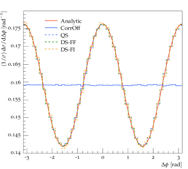
Figure 1: The analytic result for the difference in azimuthal angle between the branching planes of subsequent final-state $q\to qg$ and $g\to gg$ splittings compared to the distributions predicted using the angular-ordered (QS) and dipole parton showers in Herwig7. The predictions obtained using only final-final (DS-FF) and final-initial (DS-FI) dipoles in the dipole shower are shown separately. The prediction of the angular-ordered (CorrOff) shower without spin correlations is included for comparison. The momentum fraction in the first and second branchings lies in the range $0.9<z_{1}<1.0$ and $0.4<z_{2}<0.5$ respectively.

The analytic result for the distribution of the angular difference between the planes of successive parton shower branchings is given in Eqn. (20). This expression can be expanded for each of the four sequences of branchings that give rise to correlations using the expressions in Table 1. In this section we present the predictions of these distributions obtained using the angular-ordered and dipole parton showers in Herwig7. The angular difference between two successive parton shower branchings is measured in the splitting frame of the second branching. This test verifies the implementation of the helicity amplitudes in both parton showers. Furthermore, in the dipole shower, it also probes the implementation of the basis state mappings between splittings.

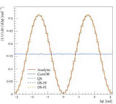
Figure 2: The analytic result for the difference in azimuthal angle between the branching planes of subsequent final-state $q\to qg$ and $g\to q\bar{q}$ splittings compared to the distributions predicted using the angular-ordered (QS) and dipole parton showers in Herwig7. The predictions obtained using only final-final (DS-FF) and final-initial (DS-FI) dipoles in the dipole shower are shown separately. The prediction of the angular-ordered (CorrOff) shower without spin correlations is included for comparison. The momentum fraction in the first and second branchings lies in the range $0.9<z_{1}<1.0$ and $0.4<z_{2}<0.5$ respectively.

We test the cases of final-state radiation (FSR) and initial-state radiation (ISR) separately. In the ISR case the first splitting is identified as that closest to the incoming hadron and the intermediate parton between the splittings is space-like. In the dipole shower we can divide FSR and ISR further according to the type of dipole considered. Specifically we divide FSR, radiation from a final-state emitter, according to whether the spectator is final-state (final-final) or initial-state (final-initial) and we divide ISR, radiation from an initial-state emitter, according to whether the spectator is final-state (initial-final) or initial-state (initial-initial). We include a separate result for each of these four types of dipole. Note that we do not consider radiation from decay processes in this test.

For the purpose of these tests we implement an artificial restriction on the splittings allowed in the dipole shower. Following the first splitting we only allow subsequent splittings from dipoles in which the spectator is the spectator of the previous splitting and in which the emitter was produced as a new parton in the previous splitting. This restriction has two purposes. First, by forbidding subsequent emissions from different legs of the hard process, it allows us to probe only the correlations in the shower. Second, by using the same spectator in subsequent splittings the frame of the second splitting is a suitable frame in which to measure the angular difference between the splittings.

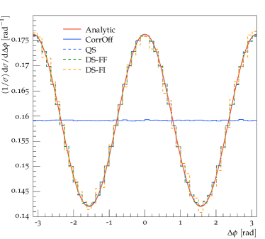
Figure 3: The analytic result for the difference in azimuthal angle between the branching planes of subsequent final-state $g\to gg$ and $g\to gg$ splittings compared to the distributions predicted using the angular-ordered (QS) and dipole parton showers in Herwig7. The predictions obtained using only final-final (DS-FF) and final-initial (DS-FI) dipoles in the dipole shower are shown separately. The prediction of the angular-ordered (CorrOff) shower without spin correlations is included for comparison. The momentum fraction in the first and second branchings lies in the range $0.9<z_{1}<1.0$ and $0.4<z_{2}<0.5$ respectively.

The results are shown in Figs. 1-4 and Figs. 6-8 for FSR and ISR respectively. We have chosen to measure the azimuthal-difference for splittings in which the momentum fraction in the first and second branchings lies in the range $0.9<z_{1}<1.0$ and $0.4<z_{2}<0.5$ respectively as this is the configuration in which the correlation is strongest. All of the results shown are for the case of massless quarks.

Each plot shows the analytic result and the parton shower predictions. In each plot we have included the prediction obtained using the angular-ordered shower with spin correlations switched off. In each case this gives rise to a flat line at $1/2\pi$ and we have confirmed that the dipole shower also predicts a flat line. All of the parton shower predictions display good agreement with the analytic result in each case.

Figure 4: The analytic result for the difference in azimuthal angle between the branching planes of subsequent final-state $g\to gg$ and $g\to q\bar{q}$ splittings compared to the distributions predicted using the angular-ordered (QS) and dipole parton showers in Herwig7. The predictions obtained using only final-final (DS-FF) and final-initial (DS-FI) dipoles in the dipole shower are shown separately. The prediction of the angular-ordered (CorrOff) shower without spin correlations is included for comparison. The momentum fraction in the first and second branchings lies in the range $0.9<z_{1}<1.0$ and $0.4<z_{2}<0.5$ respectively.

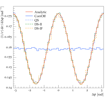
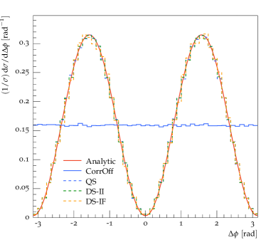
Figure 5: The analytic result for the difference in azimuthal angle between the branching planes of subsequent initial-state $q\to qg$ and $g\to gg$ splittings compared to the distributions predicted using the angular-ordered (QS) and dipole parton showers in Herwig7. The predictions obtained using only initial-initial (DS-II) and initial-final (DS-IF) dipoles in the dipole shower are shown separately. The prediction of the angular-ordered (CorrOff) shower without spin correlations is included for comparison. The momentum fraction in the first and second branchings lies in the range $0.9<z_{1}<1.0$ and $0.4<z_{2}<0.5$ respectively.

Figure 6: The analytic result for the difference in azimuthal angle between the branching planes of subsequent initial-state $q\to qg$ and $g\to q\bar{q}$ splittings compared to the distributions predicted using the angular-ordered (QS) and dipole parton showers in Herwig7. The predictions obtained using only initial-initial (DS-II) and initial-final (DS-IF) dipoles in the dipole shower are shown separately. The prediction of the angular-ordered (CorrOff) shower without spin correlations is included for comparison. The momentum fraction in the first and second branchings lies in the range $0.9<z_{1}<1.0$ and $0.4<z_{2}<0.5$ respectively.

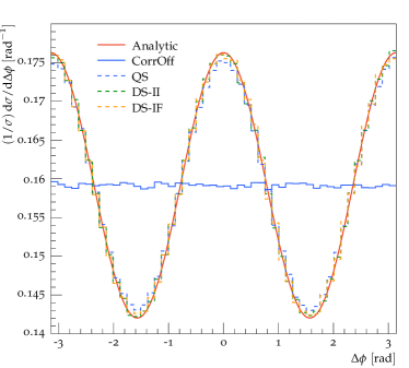
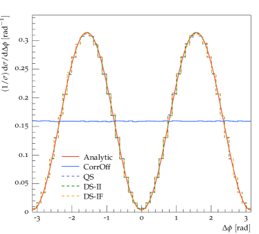
Figure 7: The analytic result for the difference in azimuthal angle between the branching planes of subsequent initial-state $g\to gg$ and $g\to gg$ splittings compared to the distributions predicted using the angular-ordered (QS) and dipole parton showers in Herwig7. The predictions obtained using only initial-initial (DS-II) and initial-final (DS-IF) dipoles in the dipole shower are shown separately. The prediction of the angular-ordered (CorrOff) shower without spin correlations is included for comparison. The momentum fraction in the first and second branchings lies in the range $0.9<z_{1}<1.0$ and $0.4<z_{2}<0.5$ respectively.

Figure 8: The analytic result for the difference in azimuthal angle between the branching planes of subsequent initial-state $g\to gg$ and $g\to q\bar{q}$ splittings compared to the distributions predicted using the angular-ordered (QS) and dipole parton showers in Herwig7. The predictions obtained using only initial-initial (DS-II) and initial-final (DS-IF) dipoles in the dipole shower are shown separately. The prediction of the angular-ordered (CorrOff) shower without spin correlations is included for comparison. The momentum fraction in the first and second branchings lies in the range $0.9<z_{1}<1.0$ and $0.4<z_{2}<0.5$ respectively.

3.2 Correlations with the Hard Process

In this section we consider results that probe the correlations between the parton shower and the hard process. These tests verify that correlations are passed correctly between the hard process and the parton shower. In addition these tests also probe the treatment of spectators and splitting recoils in the dipole shower, as discussed in Section 2.5.

The analytic result for the distribution of the azimuthal angle between the planes of the $g\to q\bar{q}$ branchings in $h^{0}\to gg\to q\bar{q}q^{\prime}\bar{q^{\prime}}$ is given in Eqn. (28). This analytic result and the predictions of the angular-ordered and dipole parton showers are shown in Fig. 9. In addition we include the result obtained from a sample of leading-order (LO) events generated using MadGraph5_aMC@NLO Alwall:2014hca . All quarks are massless and our analysis requires two gluon splittings to different quark flavours to enable perfect identification of the quark pairs. The shower predictions both display good agreement with the analytic result and the LO prediction. The differences that remain are due to the cutoff on the transverse momentum used in both parton showers, whereas the analytic result has no cutoff and the LO result includes a cut on the invariant mass of the quark-antiquark pairs which does not affect the shape of the distribution. The transverse momentum cutoff removes more of the region $z\to 0,1$ where the correlation is smallest giving a slightly larger correlation effect overall.

The above result probes the the treatment of FSR. In order to test the correlations between ISR and the hard process we also consider the Higgs boson production process $gg\to h^{0}$ followed by the backward splitting of each of the two gluons into an incoming quark and an outgoing quark. In order to obtain a finite leading-order result we require that the minimum transverse momentum of the outgoing quarks is 20 GeV.

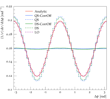
Figure 9: The analytic result for the difference in azimuthal angle between the planes of the two branchings in $h^{0}\to gg\to q\bar{q}q^{\prime}\bar{q^{\prime}}$ compared to the distributions predicted using the angular-ordered (QS) and dipole (DS) parton showers in Herwig7. The angular-ordered shower (QS-CorrOff) and dipole shower (DS-CorrOff) predictions without spin correlations are included for comparison. The result obtained from a sample of LO events generated using MadGraph5_aMC@NLO (LO) is also shown.

The predictions for the distribution of the difference in the azimuthal angle between the planes of the branchings predicted using the angular-ordered and dipole parton showers are shown in Fig. 10 and Fig. 11 respectively. In each plot we also include the result obtained from a sample of LO events generated using MadGraph5_aMC@NLO for comparison.

In Fig. 10 we include predictions obtained using the angular-ordered parton shower with and without spin correlations. When spin correlations are not included in the parton shower the predicted distribution is simply a flat line. We find that, with spin correlations included in the parton shower, the angular-ordered parton shower prediction is similar to the LO prediction with some differences in shape due to corrections beyond the collinear limit.

The predictions obtained using the dipole partonshower display more complex behaviour and we have included several results in Fig. 11. We first note that the prediction produced using the dipole parton shower without spin correlations is not flat. This is due to the treatment of splitting recoils. In initial-initial dipoles the recoil in splittings is distributed amongst all outgoing particles other than the new emission, and in initial-final dipoles the outgoing spectator gains a transverse component to its momentum. The momentum of the outgoing quark produced in the first splitting is therefore changed in a non-trivial way in the second splitting and this gives rise to a directional preference of the second splitting relative to the first splitting. This behaviour necessarily affects the prediction when spin-correlations are included and gives rise to the corresponding distribution in Fig. 11.

In order to demonstrate that the effects seen in the dipole parton shower predictions are indeed due to the treatment of recoil momenta in splittings, we have also included results obtained using a modified version of the dipole parton shower. In this modified parton shower we only allow splittings off initial-initial dipoles and we have modified the behaviour of these splittings such that the splitting recoil is entirely absorbed by the outgoing Higgs boson in both of the splittings. With these modifications the direction of the quark produced in the first splitting is not modified in the second splitting and when spin correlations are not included the predicted distribution is a flat line. As such the prediction with spin correlations included displays better agreement with the angular-ordered parton shower and LO predictions. Again there are differences in shape between the dipole parton shower prediction and the LO prediction due to corrections beyond the collinear limit.

Similar problems with the default recoil scheme indipole parton showers were recently observed in Ref. Dasgupta:2018nvj where it was shown that the same change in the recoil strategy we have used resolved issues with the logarithmic accuracy of the parton shower.

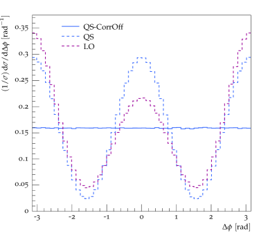
Figure 10: The difference in azimuthal angle between the planes of two initial-state $g\to q\bar{q}$ branchings in $gg\to h^{0}$ predicted using the angular-ordered (QS) parton shower in Herwig7. The angular-ordered parton shower (QS-CorrOff) prediction without spin correlations is also included. The result obtained from a sample of LO events generated using MadGraph5_aMC@NLO (LO) is shown for comparison.

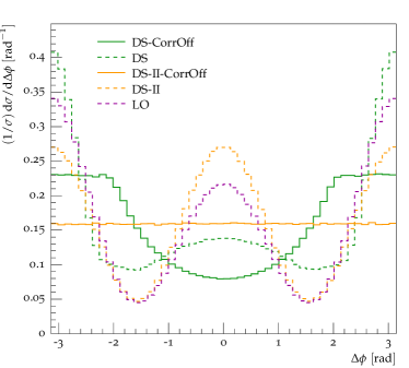
Figure 11: The difference in azimuthal angle between the planes of two initial-state $g\to q\bar{q}$ branchings in $gg\to h^{0}$ predicted using the dipole parton shower (DS) in Herwig7. The dipole parton shower (DS-CorrOff) prediction without spin correlations is also included. Predictions obtained using the dipole parton shower restricted to allow branchings from II dipoles only and with a modified handling of splitting recoils, as described in the text, are shown with (DS-II) and without (DS-II-CorrOff) spin correlations. The result obtained from a sample of LO events generated using MadGraph5_aMC@NLO (LO) is shown for comparison.

3.3 Correlations in Decay Processes

The spin correlations in the hard process can also affect the distribution of the particles produced in the subsequent decay of unstable particles, such as the top quark, and also give correlations between the decay products of different unstable particles. As we are interested in correlations in the parton shower, in this section we look at correlations in the decay of a coloured particle, namely the top quark. Fig. 12 shows the azimuthal separation of the charged leptons in dileptonic $pp\to t\bar{t}$ events at a centre-of-collision energy of 8 TeV, measured by CMS. In addition we show the predictions of this distribution obtained using the angular-ordered and dipole parton showers in Herwig7. The hard process is produced using a LO matrix element. In the angular-ordered shower the top-quark decays are corrected to NLO in QCD while in the dipole shower no such correction is applied to obtain these predictions. There is reasonable agreement between the experimental result and both parton shower algorithms including spin correlations whereas the results without spin correlations clearly fail to describe the data.

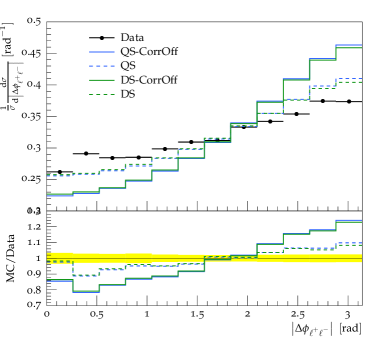
Figure 12: The azimuthal separation of the charged leptons in 8 TeV dileptonic $pp\to t\bar{t}$ events, as measured by CMS Khachatryan:2016xws and predicted using the angular-ordered (QS) and dipole (DS) parton showers in Herwig7. The predictions of the angular-ordered (QS-CorrOff) shower and the dipole shower (DS-CorrOff) without spin correlations are also shown.

4 Conclusions

We have implemented the spin correlation algorithm of Refs. Collins:1987cp ; Knowles:1987cu ; Knowles:1988hu ; Knowles:1988vs ; Richardson:2001df in the angular-ordered and dipole parton showers in Herwig7. This feature will be available for public use in Herwig7.2. We have compared the predictions obtained using each of the parton showers in Herwig7 to analytic calculations or predictions obtained using a LO ME. Through these comparisons we have confirmed that the spin correlation algorithm is functioning correctly in both showers.

The handling of splitting recoils in the dipole shower is not formally included in the spin correlation algorithm. We have discussed these limitations and presented results that show where these effects are evident. Despite these limitations, we find that the dipole shower, and the angular-ordered shower, produce a fairly accurate prediction of a spin-correlation sensitive observable, namely the azimuthal separation of the leptons, in $pp\to t\bar{t}$ events.

While spin correlation effects are often unobservable in average distributions, as we have seen there are cases where they are important. Their implementation in Herwig7 is therefore an important part of improving the accuracy of the simulation.

Appendix A Quasi-collinear Spin Unaveraged Splitting Functions

The calculation of the spin unaveraged splitting functions for $g\to q\bar{q}$ is presented in Section 2.2. We present the calculation of the remaining spin unaveraged splitting functions here.

A.1 Branching $g\to gg$

In this case $m=m_{1}=m_{2}=0$ and the polarization vectors for the outgoing gluons are:

$$\epsilon^{\mu}_{\lambda_{1}} = -\frac{\lambda_{1}}{\sqrt{2}}\left(0;1-{\frac{p_{\perp}^{2}\lambda^{2}{\rm e}^{i\lambda_{1}\phi}\cos\phi}{2{{\bf p}}^{2}{z}^{2}}},\right.$$

$$\ \ \ \ \ \ \ \ \ \left.i\lambda_{1}-{\frac{{p_{\perp}}^{2}\lambda^{2}{\rm e}^{i\lambda_{1}\phi}\sin\phi}{2{\bf p}^{2}z^{2}}},-\frac{p_{\perp}{\rm e}^{i\lambda_{1}\phi}}{{\bf p}z}\lambda\right)+\mathcal{O}(\lambda^{3});$$

$$\epsilon^{\mu}_{\lambda_{2}} = -\frac{\lambda_{2}}{\sqrt{2}}\left(0;1-\frac{p_{\perp}^{2}\lambda^{2}{\rm e}^{i\lambda_{2}\phi}\cos\phi}{2{\bf p}^{2}\left(1-z\right)^{2}},\right.$$

$$\ \ \ \ \ \ \ \ \ \left.i\lambda_{2}-\frac{p_{\perp}^{2}\lambda^{2}{\rm e}^{i\lambda_{2}\phi}\sin\phi}{2{\bf p}^{2}\left(1-z\right)^{2}},\frac{p_{\perp}{\rm e}^{i\lambda_{2}\phi}}{\left(1-z\right){\bf p}}\lambda\right)+\mathcal{O}(\lambda^{3}).$$

The helicity amplitudes for the branching can be written as

$$F_{\lambda_{0}\lambda_{1}\lambda_{2}} = \sqrt{\frac{2}{q^{2}_{0}}}\left[q_{1}\cdot\epsilon^{*}_{2}\epsilon_{0}\cdot\epsilon^{*}_{1}-q_{1}\cdot\epsilon_{0}\epsilon^{*}_{1}\cdot\epsilon^{*}_{2}-q_{2}\cdot\epsilon^{*}_{1}\epsilon_{0}\cdot\epsilon^{*}_{2}\right],$$

$$= -\frac{1}{2}\sqrt{z(1-z)}e^{i(\lambda_{0}-\lambda_{1}-\lambda_{2})\phi^{\prime}}$$

$$\left[\lambda_{0}\lambda_{1}\lambda_{2}\left(\frac{1}{z(1-z)}-1\right)+\lambda_{0}+\frac{\lambda_{1}}{z}+\frac{\lambda_{2}}{1-z}\right].$$

This function gives the correct spin averaged splitting function and also is the same as the splitting functions used in Herwig6 from Knowles:1987cu  Table 1. The results for the individual helicity states are given in Table 2.

$\lambda_{0}$	$\lambda_{1}$	$\lambda_{2}$	$g\to gg$	$g\to q\bar{q}$
+	+	+	$-{\frac{1}{\sqrt{z\left(1-z\right)}}}$	${\frac{m}{z\left(1-z\right)\tilde{q}}}$
+	+	-	${\frac{{z}^{3/2}}{\sqrt{1-z}}}$	$z\sqrt{1-{\frac{{m}^{2}}{{z}^{2}\left(1-z\right)^{2}\tilde{q}^{2}}}}$
+	-	+	${\frac{\left(1-z\right)^{3/2}}{\sqrt{z}}}$	$-\left(1-z\right)\sqrt{1-{\frac{{m}^{2}}{{z}^{2}\left(1-z\right)^{2}\tilde{q}^{2}}}}$
+	-	-	$0$	$0$
-	+	+	$0$	$0$
-	+	-	$-{\frac{\left(1-z\right)^{3/2}}{\sqrt{z}}}$	$\left(1-z\right)\sqrt{1-{\frac{{m}^{2}}{{z}^{2}\left(1-z\right)^{2}\tilde{q}^{2}}}}$
-	-	+	$-{\frac{{z}^{3/2}}{\sqrt{1-z}}}$	$-z\sqrt{1-{\frac{{m}^{2}}{{z}^{2}\left(1-z\right)^{2}\tilde{q}^{2}}}}$
-	-	-	${\frac{1}{\sqrt{z\left(1-z\right)}}}$	${\frac{m}{z\left(1-z\right)\tilde{q}}}$

Table 2: Spin unaveraged splitting functions for $g\to gg$ and $g\to q\bar{q}$. In addition to the factors given above each term has a phase $e^{i\phi^{\prime}(\lambda_{0}-\lambda_{1}-\lambda_{2})}$, where $\lambda_{1,2}=\pm 1$ for outgoing gluons and $\lambda_{1,2}=\pm\frac{1}{2}$ for outgoing quarks. For the $g\to q\bar{q}$ splitting function $\tilde{q}$ is the Herwig7 evolution variable.

A.2 Quark and Antiquark Branching

For quarks and antiquarks there is only one branching to consider, i.e. $q\to qg$. In this case $m_{0}=m_{1}=m$ and $m_{2}=0$. This gives the spinors:

$$u_{\frac{1}{2}}(p) = \left(\begin{array}[]{c}\frac{m}{\sqrt{2{\bf p}}}\lambda\\ 0\\ \sqrt{2{\bf p}}\left(1+\frac{m^{2}\lambda^{2}}{8{\bf p}^{2}}\right)\\ 0\end{array}\right);$$ (32e)

$$u_{-\frac{1}{2}}(p) = \left(\begin{array}[]{c}0\\ \sqrt{2{\bf p}}\left(1+\frac{m^{2}\lambda^{2}}{8{\bf p}^{2}}\right)\\ 0\\ \frac{m}{\sqrt{2{\bf p}}}\lambda\end{array}\right).$$ (32j)

The polarization vectors of the gluon are

$$\epsilon^{\mu}_{\lambda_{2}}(q_{2}) = \left[0;-\frac{\lambda_{2}}{\sqrt{2}}\left(1-\frac{p_{\perp}^{2}\lambda^{2}{\rm e}^{i\lambda_{2}\phi}\cos\phi}{2{\bf p}^{2}\left(1-z\right)^{2}}\right),\right.$$ (33)

$$\!\!\!\!\!\left.-\frac{i}{\sqrt{2}}+\frac{\lambda_{2}p_{\perp}^{2}\lambda^{2}{\rm e}^{i\phi}\sin\phi}{2\sqrt{2}{\bf p}^{2}\left(1-z\right)^{2}},-\frac{\lambda_{2}p_{\perp}\lambda{\rm e}^{i\lambda_{2}\phi}}{\sqrt{2}\left(1-z\right){\bf p}}\right]\!\!.$$

and the spinors of the outgoing quark:

$$\bar{u}_{\frac{1}{2}}(q_{1}) = \left[\sqrt{2z{\bf p}}\left(1+\frac{m^{2}\lambda^{2}}{8{\bf p}^{2}}\right),\frac{{\rm e}^{-i\phi}p_{\perp}\lambda}{\sqrt{2z{\bf p}}},\right.$$ (34a)

$$\ \ \ \ \ \left.\frac{m}{\sqrt{2z{\bf p}}}\lambda,\frac{{\rm e}^{-i\phi}p_{\perp}m{\lambda}^{2}}{2z{\bf p}\sqrt{2z{\bf p}}}\right]\!;$$

$$\bar{u}_{-\frac{1}{2}}(q_{1}) = \left[-\frac{{\rm e}^{i\phi}p_{\perp}m\lambda^{2}}{2z{\bf p}\sqrt{2z{\bf p}}},\frac{m}{\sqrt{2z{\bf p}}}\lambda,\right.$$ (34b)

$$\ \ \ \ \ \left.-\frac{{\rm e}^{i\phi}p_{\perp}\lambda}{\sqrt{2z{\bf p}}},\sqrt{2z{\bf p}}\left(1+\frac{m^{2}\lambda^{2}}{8z{\bf p}}\right)\right]\!.$$

In this case the helicity amplitudes for the branching are

$$F_{\lambda_{0}\lambda_{1}\lambda_{2}}=\sqrt{\frac{1}{2(q^{2}_{0}-m^{2})}}\bar{u}_{\lambda_{1}}(q_{1})\epsilon_{\lambda_{2}}\!\!\!\!\!\!\!\!\!\!\not\,\,\,\,\,\,\,u_{\lambda_{0}}(q_{0}).$$ (35)

These functions are given in Table 3.

		$F_{\lambda_{0},\lambda_{1},\lambda_{2}}$
$\lambda_{0}$	$\lambda_{1}$	$\lambda_{2}=+$	$\lambda_{2}=-$
+	+	${\frac{1}{\sqrt{1-z}}\sqrt{1-{\frac{{m}^{2}}{{z}^{2}{\tilde{q}}^{2}}}}}$	$-{\frac{z}{\sqrt{1-z}}\sqrt{1-{\frac{{m}^{2}}{{z}^{2}{\tilde{q}}^{2}}}}}$
+	-	$\frac{m}{\tilde{q}}\frac{\sqrt{1-z}}{z}$	$0$
-	+	$0$	$\frac{m}{\tilde{q}}\frac{\sqrt{1-z}}{z}$
-	-	${\frac{z}{\sqrt{1-z}}\sqrt{1-{\frac{{m}^{2}}{{z}^{2}{\tilde{q}}^{2}}}}}$	$-{\frac{1}{\sqrt{1-z}}\sqrt{1-{\frac{{m}^{2}}{{z}^{2}{\tilde{q}}^{2}}}}}$

Table 3: Spin unaveraged splitting functions for $q\to qg$. In addition to the factors given above each term has a phase $e^{i\phi^{\prime}(\lambda_{0}-\lambda_{1}-\lambda_{2})}$, where $\lambda_{2}=\pm 1$ for the outgoing gluon and $\lambda_{0,1}=\pm\frac{1}{2}$ for quarks and $\tilde{q}$ is the Herwig++ evolution variable.

A.3 Squark Branching

For squarks there is only one branching to consider, i.e. $\tilde{q}\to\tilde{q}g$. The kinematics are the same as those for gluon radiation from a quark, i.e. $m_{0}=m_{1}=m$ and $m_{2}=0$. The polarization vectors of the gluons are also the same as for radiation from a quark, Eqn. 33.

The spin unaveraged splitting function is given by

$$F_{\lambda_{2}} = \sqrt{\frac{2}{q^{2}_{0}-m^{2}}}q_{1}\cdot\epsilon_{2}^{*}$$ (36)

$$= \lambda_{2}e^{-i\lambda_{2}\phi^{\prime}}\sqrt{1-\frac{m^{2}}{z^{2}\tilde{q}^{2}}}\sqrt{\frac{z}{1-z}}.$$

If we sum over the helicities of the gluon we obtain the correct massive splitting function.

Appendix B Basis Rotation

In the case that we have a spin density matrix from the production process and then wish to generate the correlations in the shower for simplicity we will have to deal with the rotation of the basis states used.

Consider a process with production matrix element $\mathcal{A}_{\rm prod}$ and a matrix element $\mathcal{A}_{\rm branch}$ giving the subsequent time-like branching of the intermediate particle with momentum $p$ and mass $m$.

In the case of a fermion we will replace the spin sum with the Dirac spin sum, i.e

$$p\!\!\!\!\!\not\>\>\!+m=\sum_{a}\Psi_{a}\bar{\Psi}_{a},$$ (37)

or similarly for vector bosons

$$-g^{\mu\nu}+\frac{p^{\mu}n^{\nu}+p^{\nu}n^{\mu}}{p\cdot n}=\sum_{a}\epsilon_{a}^{\mu}\epsilon_{a}^{*\nu}$$ (38)

We write both of these as

$$\sum_{a}\chi_{a}\chi_{a}^{\dagger},$$ (39)

where the basis state for the production is $\chi^{\dagger}_{a}$ and for the branching is $\chi_{a}$ such that the matrix element for the full process is

$$\mathcal{M}=\mathcal{A}_{\rm branch}\chi_{a}\chi_{a}^{\dagger}\mathcal{A}_{\rm prod},$$ (40)

using the Einstein convention.

The matrix element squared is then

$$|\overline{\mathcal{M}}|^{2}=\chi^{\dagger}_{b}\mathcal{A}^{\dagger}_{\rm branch}\mathcal{A}_{\rm branch}\chi_{a}\chi_{a}^{\dagger}\mathcal{A}_{\rm prod}\mathcal{A}^{\dagger}_{\rm prod}\chi_{b}$$ (41)

If we normalise by the spin summed matrix element for the production process then we obtain

$$\frac{|\overline{\mathcal{M}|^{2}}}{\overline{|\mathcal{M}_{\rm prod}|^{2}}}=\rho_{ab}\chi^{\dagger}_{b}\mathcal{A}^{\dagger}_{\rm branch}\mathcal{A}_{\rm branch}\chi_{a},$$ (42)

where $\mathcal{M}_{\rm prod}=\chi_{a}^{\dagger}\mathcal{A}_{\rm prod}$ and

$$\rho_{ab}=\frac{1}{\overline{|\mathcal{M}_{\rm prod}|^{2}}}\chi_{a}^{\dagger}\mathcal{A}_{\rm prod}\mathcal{A}^{\dagger}_{\rm prod}\chi_{b}.$$ (43)

In order to simplify the calculation we have made a specific choice of the basis of the wavefunctions $\chi^{\prime}_{a}$ when we calculate the branching, which may not be the same as those used in the calculation of the production, $\chi_{a}$, after Lorentz transformation into the frame in which the branching is calculated.

We therefore need to calculate the rotation between these two choices of basis states

$$\chi_{a}=\omega_{ai}\chi^{\prime}_{i},$$ (44)

therefore the calculation of the distribution is given by

$$\frac{|\overline{\mathcal{M}|^{2}}}{\overline{|\mathcal{M}_{\rm prod}|^{2}}} = \omega_{ai}\rho_{ab}\omega^{*}_{bj}\chi^{\prime\dagger}_{j}\mathcal{A}^{\dagger}_{\rm branch}\mathcal{A}_{\rm branch}\chi^{\prime}_{i}$$

$$= \rho^{\prime}_{ij}\chi^{\prime\dagger}_{j}\mathcal{A}^{\dagger}_{\rm branch}\mathcal{A}_{\rm branch}\chi^{\prime}_{i},=\rho^{\prime}_{ij}\mathcal{M}^{\dagger}_{{\rm branch}j}\mathcal{M}_{{\rm branch}i}$$

where

$$\rho^{\prime}_{ij}=\omega_{ai}\rho_{ab}\omega^{*}_{bj}$$ (46)

and $\mathcal{M}_{{\rm branch}i}=\mathcal{A}_{\rm branch}\chi^{\prime}_{i}$.

If we consider the case of space-like branching then the incoming particle to the hard process will now have basis state $\chi_{a}$ and outgoing particle from the space-like branching $\chi^{\dagger}_{a}$ such that the matrix element is

$$\mathcal{M}=\mathcal{A}_{\rm prod}\chi_{a}\chi_{a}^{\dagger}\mathcal{A}_{\rm branch},$$ (47)

The matrix element squared is then

$$|\overline{\mathcal{M}}|^{2}=\chi^{\dagger}_{b}\mathcal{A}^{\dagger}_{\rm prod}\mathcal{A}_{\rm prod}\chi_{a}\chi_{a}^{\dagger}\mathcal{A}_{\rm branch}\mathcal{A}^{\dagger}_{\rm branch}\chi_{b}$$ (48)

If we normalise by the spin summed matrix element for the production process then we obtain

$$\frac{|\overline{\mathcal{M}|^{2}}}{\overline{|\mathcal{M}_{\rm branch}|^{2}}}=D_{ab}\chi^{\dagger}_{a}\mathcal{A}_{\rm branch}\mathcal{A}^{\dagger}_{\rm branch}\chi_{b},$$ (49)

where in this case $\mathcal{M}_{\rm prod}=\mathcal{A}_{\rm prod}\chi_{a}$ and

$$D_{ab}=\frac{1}{\overline{|\mathcal{M}_{\rm prod}|^{2}}}\chi^{\dagger}_{b}\mathcal{A}^{\dagger}_{\rm prod}\mathcal{A}_{\rm prod}\chi_{a}.$$ (50)

If we then rotate the basis states as before the calculation of the distribution is given by

$$\frac{|\overline{\mathcal{M}|^{2}}}{\overline{|\mathcal{M}_{\rm prod}|^{2}}} = \omega_{bj}D_{ab}\omega^{*}_{ai}\chi^{\prime^{\dagger}}_{i}\mathcal{A}_{\rm branch}\mathcal{A}^{\dagger}_{\rm branch}\chi^{\prime}_{j}$$

$$= D^{\prime}_{ij}\chi^{\prime^{\dagger}}_{i}\mathcal{A}_{\rm branch}\mathcal{A}^{\dagger}_{\rm branch}\chi^{\prime}_{j}=D^{\prime}_{ij}\mathcal{M}_{{\rm branch}i}\mathcal{M}^{\dagger}_{{\rm branch}j}$$

where

$$D^{\prime}_{ij}=\omega_{bj}D_{ab}\omega^{*}_{ai}$$ (52)

and $\mathcal{M}_{{\rm branch}i}=\chi^{\prime^{\dagger}}_{i}\mathcal{A}_{\rm branch}$.

References

• (1) A. Buckley et al., Phys. Rept. 504, 145 (2011), 1101.2599.
• (2) K. Kato and T. Munehisa, Phys. Rev. D36, 61 (1987).
• (3) K. Kato and T. Munehisa, Phys. Rev. D39, 156 (1989).
• (4) K. Kato and T. Munehisa, Comput. Phys. Commun. 64, 67 (1991).
• (5) K. Kato, T. Munehisa, and H. Tanaka, Z. Phys. C54, 397 (1992).
• (6) W. T. Giele, D. A. Kosower, and P. Z. Skands, Phys. Rev. D84, 054003 (2011), 1102.2126.
• (7) L. Hartgring, E. Laenen, and P. Skands, JHEP 10, 127 (2013), 1303.4974.
• (8) H. T. Li and P. Skands, Phys. Lett. B771, 59 (2017), 1611.00013.
• (9) S. Höche, F. Krauss, and S. Prestel, JHEP 10, 093 (2017), 1705.00982.
• (10) S. Höche and S. Prestel, Phys. Rev. D96, 074017 (2017), 1705.00742.
• (11) F. Dulat, S. Höche, and S. Prestel, (2018), 1805.03757.
• (12) S. Plätzer and M. Sjodahl, JHEP 07, 042 (2012), 1201.0260.
• (13) R. A. Martínez, M. De Angelis, J. R. Forshaw, S. Plätzer, and M. H. Seymour, (2018), 1802.08531.
• (14) J. C. Collins, Nucl. Phys. B304, 794 (1988).
• (15) I. G. Knowles, Nucl. Phys. B304, 767 (1988).
• (16) I. G. Knowles, Comput. Phys. Commun. 58, 271 (1990).
• (17) I. G. Knowles, Nucl. Phys. B310, 571 (1988).
• (18) P. Richardson, JHEP 11, 029 (2001), hep-ph/0110108.
• (19) G. Corcella et al., JHEP 01, 010 (2001), hep-ph/0011363.
• (20) D. J. Lange, Nucl. Instrum. Meth. A462, 152 (2001).
• (21) M. Bähr et al., Eur. Phys. J. C58, 639 (2008), 0803.0883.
• (22) J. Bellm et al., Eur. Phys. J. C76, 196 (2016), 1512.01178.
• (23) J. Bellm et al., (2017), 1705.06919.
• (24) S. Catani, S. Dittmaier, and Z. Trocsanyi, Phys. Lett. B500, 149 (2001), hep-ph/0011222.
• (25) S. Gieseke, P. Stephens, and B. Webber, JHEP 12, 045 (2003), hep-ph/0310083.
• (26) H. E. Haber, (1994), hep-ph/9405376.
• (27) S. Platzer and S. Gieseke, Eur. Phys. J. C72, 2187 (2012), 1109.6256.
• (28) S. Catani and M. H. Seymour, Nucl. Phys. B485, 291 (1997), hep-ph/9605323, [Erratum: Nucl. Phys.B510,503(1998)].
• (29) S. Catani, S. Dittmaier, M. H. Seymour, and Z. Trocsanyi, Nucl. Phys. B627, 189 (2002), hep-ph/0201036.
• (30) J. Alwall et al., JHEP 07, 079 (2014), 1405.0301.
• (31) M. Dasgupta, F. A. Dreyer, K. Hamilton, P. F. Monni, and G. P. Salam, (2018), 1805.09327.
• (32) CMS, V. Khachatryan et al., Phys. Rev. D93, 052007 (2016), 1601.01107.