Reflection Spectroscopy of the Black Hole Binary XTE J1752–223 in its Long-Stable Hard State

Abstract

We present a detailed spectral analysis of the Black Hole Binary XTE J1752–223 in the hard state of its 2009 outburst. Regular monitoring of this source by RXTE provided high signal-to-noise spectra along the outburst rise and decay. During one full month this source stalled at $\sim$30% of its peak count rate at a constant hardness and intensity. By combining all the data in this exceptionally-stable hard state, we obtained an aggregate PCA spectrum (3–45 keV) with 100 million counts, and a corresponding HEXTE spectrum (20–140 keV) with 5.8 million counts. Implementing a version of our reflection code with a physical model for Comptonization, we obtain tight constraints on important physical parameters for this system. In particular, the inner accretion disk is measured very close in, at $R_{\mathrm{in}}=1.7\pm 0.4$ $R_{g}$. Assuming $R_{\mathrm{in}}=R_{\mathrm{ISCO}}$, we find a relatively high black hole spin ($a_{*}=0.92\pm 0.06$). Imposing a lamppost geometry, we obtain a low inclination ($i=35\pm 4$ deg), which agrees with the upper limit found in the radio ($i<49$ deg). However, we note that this model cannot be statistically distinguished from a non-lamppost model with free emissivity index, for which the inclination is markedly higher. Additionally, we find a relatively cool corona ($57-70$ keV), and large iron abundance ($3.3-3.7$ solar). We further find that properly accounting for Comptonization of the reflection emission improves the fit significantly and causes an otherwise low reflection fraction ($\sim 0.2-0.3$) to increase by an order of magnitude, in line with geometrical expectations for a lamppost corona. We compare these results with similar investigations reported for GX 339–4 in its bright hard state.

1. Introduction

Accreting black holes are unique probes of physics under the conditions of extreme gravity. Supermassive black holes at the centers of galaxies shape their hosts through their powerful outflows (Fabian, 2012), and their smaller cousins, black hole binaries (BHBs), may have played an important role during the epoch of ionization (e.g.; Madau & Fragos, 2017). Accretion processes in supermassive black holes are, however, hard to study because of their long variability timescale and large distances that result in low fluxes. Luckily, timescales of key accretion and ejection processes scale with mass, so that BHBs can be seen as supermassive black holes on fast-forward, with whole outburst cycles occurring within mere months or years.

Typical BHBs spend most of their time in quiescence. They start an outburst in the hard state, when the source spectrum is dominated by hard X-rays in the form of a power-law component with photon index $\Gamma\sim 1.7$. In this state, there is little or no contribution from thermal accretion-disk emission. Radio emission is detected and, for some sources, collimated outflows have been resolved (e.g.; Mirabel & Rodríguez, 1999). The source brightness increases at almost constant hardness until the spectrum finally begins to soften both in photon index and through stronger contribution from the accretion disk in the soft X-rays: the source enters first the hard-intermediate and then the soft-intermediate states. It finally reaches the soft state (also referred to as the thermal state), when the X-ray continuum is dominated by the accretion disk emission and the power-law component is steep ($\Gamma\gtrsim 2$). Radio emission in the soft state is strongly suppressed. In a typical outburst, the source dims over months in the thermal state, and at lower luminosity returns through intermediate states back to a hard state in which it fades back into quiescence (see McClintock & Remillard, 2006; Remillard & McClintock, 2006, for reviews).

While the phenomenology itself is rather well described, its physical underpinning remains a mystery. In particular, the geometry of the emission region is unclear: the power law is likely produced through thermal Comptonization and further modified through reflection off the accretion disk, but the origin of this Comptonizing medium—often referred to as the corona—whether it is due to inverse Compton (IC) scattering of disk photons in a hot and static plasma (e.g.; Haardt, 1993; Dove et al., 1997; Zdziarski et al., 2003), or whether it is due to IC scattering within the base of a jet (e.g.; Matt et al., 1992; Markoff et al., 2005), is still under debate. Observationally, the slope of the power-law continuum and its cutoff at high energies provide direct information on the temperature and optical depth of the corona, and, somewhat more loose constraints on its geometry (Fabian et al., 2015, 2017); and have an important effect on the shape of the reflection spectrum (García et al., 2013, 2015a).

XTE J1752–223 is an X-ray transient discovered in 2009 October 23 by the All Sky Monitor (ASM) on board the Rossi X-ray Timing Explorer (RXTE) (Markwardt et al., 2009b). Intense monitoring of its 2009 outburst (the only one detected to date) with RXTE, Swift, and MAXI indicated that the source is a BHB candidate (Markwardt et al., 2009a; Nakahira et al., 2009; Remillard & ASM Team at MIT, 2009; Shaposhnikov et al., 2009, 2010; Shaposhnikov, 2010). Radio and X-ray jets have been detected in this source, including ballistic jets observed in the radio, which are typically associated with hard-to-soft state transitions (generally during the intermediate or steep power-law states; Brocksopp et al., 2010; Yang et al., 2010, 2011; Brocksopp et al., 2013). Shaposhnikov et al. (2010) applied correlations between spectral and variability properties for XTE J1550–564 and GRO J1655–40 in order to estimate a mass for XTE J1752–223 of $9.6\pm 0.8$ $M_{\odot}$, and a distance of $3.5\pm 0.4$ kpc. However, these quantities have not been verified and notably there is no dynamical mass constraint. An inclination upper limit of $i<49$ deg was found using photometric observations of the radio jet during the transition from the hard to the soft state (Miller-Jones et al., 2011).

In this paper, we present a detailed spectroscopic analysis of the hard state of XTE J1752–223. RXTE pointed observations showed a protracted month-long period in which the luminosity and hardness ratio of the source were found to be extraordinarily stable, resulting in a unique dataset of exceptional quality among stellar-mass black hole systems. Following the methodology developed previously for GX 339–4 (García et al., 2015b), we combined these 300 ks of stable hard-state data into a single spectrum with $\sim 100$ million source counts ($\sim$3–140 keV). Using a newly improved version of our relativistic reflection model that includes a physical Comptonization continuum (relxillCp; García & Dauser, 2018), we derived precise constraints on the black hole spin, the inner radius of the disk, the inclination of the reflector, the ionization state and iron abundance of the disk’s atmosphere, and the temperature and optical depth of the corona.

This paper is organized as follows: In Section 2 we describe the observational data; the spectral analysis is presented in Section 3. We discuss the main implications of our results in Section 4, and offer concluding remarks in Section 5.

Figure 1.— (Top) Hardness-intensity diagram for GX 339–4 (grey circles) and XTE J1752–223 (red dots). The X-ray hardness in the horizontal axis is defined as the ratio of the source counts at 8.6–18 keV to the counts at 5–8.6 keV (Remillard & McClintock, 2006), after correcting to stabilize variations in the Crab rates to account for gain drift. The PCU-2 count rate has been normalized to the Crab following Peris et al. (2016), taking into account possible flux variations (Wilson-Hodge et al., 2011). All the hard-state data shown inside the box (light red) are combined into a single, high signal-to-noise spectrum, equivalent to a $\sim 3\times 10^{5}$ s exposure with a total of 100 million counts. (Middle, Bottom) PCA light curve and hardness ratio as a function of time throughout the outburst. The gap between MJDs $\sim 55160-55210$ shows a Sun exclusion period.

2. Observations

We have analyzed the RXTE archival data for the hard state of XTE J1752–223, specifically, all 6 observations from proposal ID P94044, and the first 51 observations from proposal ID P94331 starting with ObsID 94331-01-01-00 up to ObsID 94331-01-05-00. This includes spectra taken with the Proportional Counter Array (PCA; Jahoda et al., 2006), a set of five proportional counter detectors sensitive over the energy range 2–60 keV; and spectra taken with the the High Energy X-ray Timing Experiment (HEXTE; Rothschild et al., 1998), a set of two independent clusters (A and B), each with four NaI(Tl)/CsI(Na) phoswich scintillation detectors sensitive over the 15–250 keV energy range. We followed the standard extraction procedure for both PCA and HEXTE as outlined in Grinberg et al. (2013), but used HEASOFT 6.16 and all Xenon layers for the PCA extraction. We extracted one spectrum for each ObsID: for PCA, we used standard2f PCU 2 spectra, discarding data within 10 min from the South Atlantic Anomaly. For HEXTE, we only extracted data from cluster B due to the failure of cluster A earlier in the mission. As done in García et al. (2016), the HEXTE data was grouped beyond the standard reduction procedure by factors of 2, 3, and 4, in the energy ranges of 20–30 keV, 30–40 keV, and 40–250 keV, respectively, in order to achieve an over-sampling of $\sim 3$ times the instrumental resolution.

Figure 2.— Count spectra of the combined PCA (light blue) and HEXTE (gold) data for the hard-state of XTE J1752–223. The grey symbols show the background for each data set.

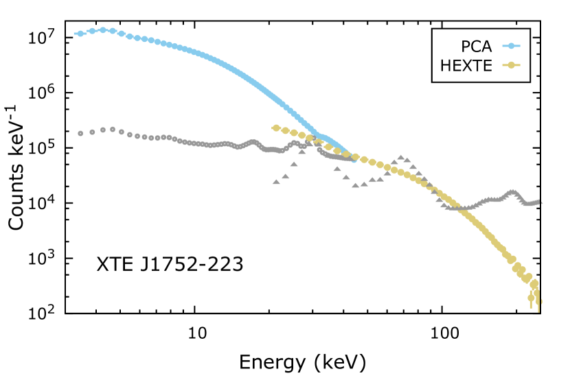
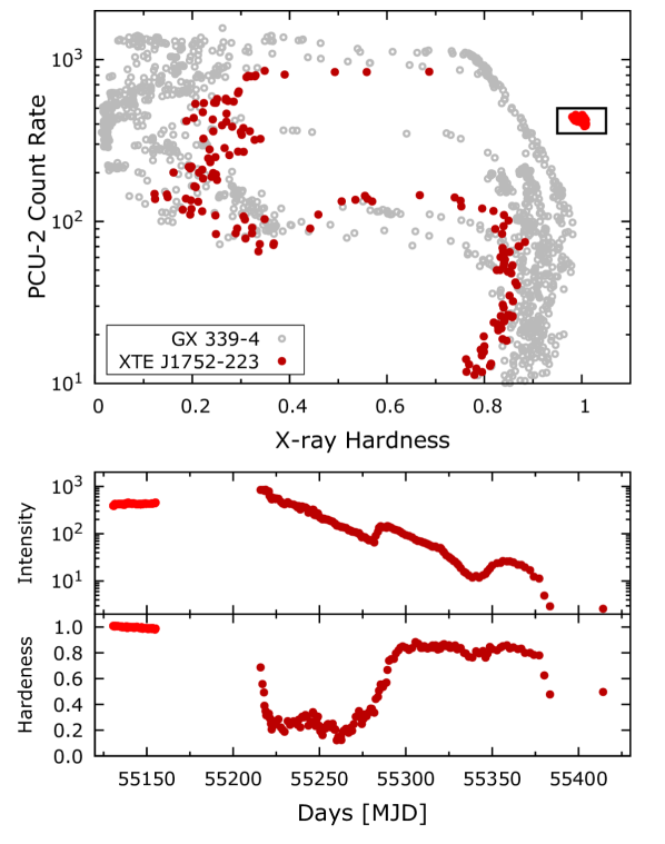
Figure 1 (top) shows the standard hardness-intensity diagram (Homan & Belloni, 2005) for the 2009 outburst of XTE J1752–223 (red points), together with the multi-outburst data of the prototypical BHB GX 339–4 (grey circles). Unlike GX 339–4, XTE J1752–223 displayed a nearly constant intensity (about 30% of its peak rate), for roughly a full month during the rise phase in the hard state, corresponding to the concentration of points in the upper-right region of the diagram, indicated inside the box (light red dots). These very stable hard-state data were combined into a single spectrum following the procedures described in García et al. (2015b) for GX 339–4. A total of 57 individual pointings taken during MJD 55130–55155 were combined into a unique dataset of exceptional quality: a total of 300 ks were combined into a single PCA (3–45 keV) spectrum with 100 million counts, and a single HEXTE spectrum (20–250 keV) with 10 million counts. Middle and lower panels of Figure 1 show the light curve and hardness ratio as function of time for XTE J1752–223, respectively. The gap between the hard-state observations (light red) and the transition to the soft state (darker red), is due to a Sun exclusion period.

Figure 3.— Ratio plot (left) and contribution to $\chi^{2}$ (right) from the different model fits. The model used is show in the left panels, and the corresponding $\chi_{\nu}^{2}$ is indicated in the right panels.

The final PCA spectrum was further calibrated with our correction tool pcacorr (García et al., 2014b), which improves the data quality and accordingly enhances the detector sensitivity to more subtle spectral features such as the Fe K line and edge. Mere 0.1% systematic uncertainties are sufficient after this correction for analyzing the PCA dataset. Given that all the HEXTE observations for XTE J1752–223 were taken with the Cluster B, we have also corrected the final HEXTE spectrum with the hexBcorr tool, as described in García et al. (2016). No systematics are included to the HEXTE spectra.

The net spectra for both PCA and HEXTE are shown in Figure 2, including their corresponding backgrounds. The HEXTE background becomes dominant at high energies, above $\sim$100 keV. At 250 keV the background is more than a factor of ten higher than the source counts. We thus limit our analysis up to 140 keV, where the background counts are no higher than 50% the source counts. In the analyzed HEXTE range (20–140 keV), there are 5.8 million counts.

3. Spectral Analysis

3.1. Exploration: Empirical Determination of the Model Components

The spectral analysis of the combined hard-state data for XTE J1752–223 is carried out by simultaneously fitting the PCA and HEXTE spectra. For the PCA spectra, channels 1–4 and energies above 45 keV are ignored. For the HEXTE spectra, we only consider the 20–140 keV range. The fitting and statistical analysis was carried out using the xspec package v-12.9.0d (Arnaud, 1996).

The present analysis follows closely our previous work on the hard state of GX 339–4 (García et al., 2015b). However, there are two important methodological differences here: (i) we included simultaneous high-energy data provided by HEXTE, which has been corrected with our hexBcorr tool (García et al., 2016); and (ii) we have updated our reflection models to now include a physically motivated Comptonization continuum.

Table 1Statistics for the progression of initial model fits

Model	$\chi^{2}$	$\nu$	$\chi^{2}_{\nu}$	$\Delta\chi^{2}/\Delta\nu$
const*TBabs*cutoffpl	27932.32	102	273.85
const*TBabs*nthComp	9097.31	102	89.19	18835.01
const*TBabs*relxillCp	233.83	97	2.41	8863.48
const*TBabs*(relxillCp+xillverCp); ($q=3$)	199.32	96	2.08	34.51
const*TBabs*(relxillCp+xillverCp); (Free $q$)	175.00	95	1.84	24.32
const*TBabs*(relxillCp+xillverCp+gau+gau); (Free $q$)	127.49	92	1.39	15.70

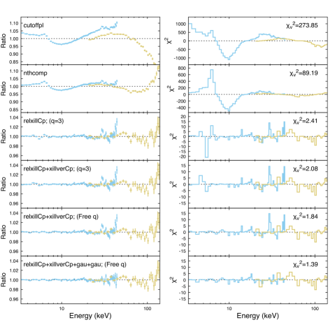
Figure 3 shows the residuals resulting from a progression of models applied to the XTE J1752–223 data, which sequentially increment in complexity. The statistics of each fit are summarized in Table 1. For all models, a normalization constant is included to account for the differences in the flux calibration between the PCA and the HEXTE instruments. Galactic absorption is included by implementing the TBabs model with the corresponding abundances as set by Wilms et al. (2000), and the Verner et al. (1996) photoelectric cross sections.

We first start with a simple model for the continuum in the form of a power law with an exponential cutoff at high energies (i.e., cutoffpl). Very large residuals can be seen in the top panels of Figure 3, which resemble the signatures of reprocessing from an optically-thick material in the form of a broad Fe K emission line at $\sim$6.6 keV, a smeared Fe K edge at $\sim$8 keV, and a broad Compton hump peaking at $\sim$30 keV. Despite the inclusion of a cross calibration constant, this model fails to correctly describe the curvature at high energies and thus there appears to be a mismatch between the two spectra.

The presence of a power-law continuum with a high-energy cutoff is commonly attributed to the emission from an optically-thin, hot Comptonizing corona (e.g.; Done et al., 2007). Thus, we replace the e-folded power-law model with a physically motivated thermal Comptonization model nthComp, included as part of xspec. This model, developed by Zdziarski et al. (1996) and later extended by Życki et al. (1999), provides a more accurate description of the cutoff at high energies, which is sharper than the exponential cutoff. In this prescription, the seed photons from the thermal disk emission (a quasi blackbody) are Compton up-scattered by the hot electrons in the corona. The residuals of this fit are shown in the second panels of Figure 3. This model provides a significantly better match to the data bringing the reduced chi-square from 274 to 89, and providing a better agreement between the two datasets in the spectral region where they overlap (20–45 keV). In this case, the high energy cutoff is much sharper than the exponential, which not only affects the shape of the continuum but also the shape of the reflected spectrum, as we describe next.

To model the residuals observed we then make use of our suite of relativistic reflection models relxill (v-0.4j) (García et al., 2014a; Dauser et al., 2014). This model is the result of the merging of the ionized reflection spectra produced with the xillver code (García & Kallman, 2010; García et al., 2011, 2013), with the ray tracing calculations based on the relativistic convolution kernel relline (Dauser et al., 2010, 2013). The relxill models properly take into account the angular dependence of the reflection as a function of the radius in the accretion disk, including the most recent dataset of atomic quantities. The relativistic effects that smear and modify the spectrum are included considering two basic geometries: the extended corona (in the standard relxill), assuming that the emissivity of the disk follows a powerlaw with the radius $\propto r^{-q}$, with the index $q$ being a fit parameter; and the lamppost corona (in relxilllp), assuming a point-like source at the rotation axis above the black hole (with the height $h$ being a fit parameter). In all cases, the model provides both the illuminating continuum and the reflected spectrum for a given set of parameters. The shape of the continuum can be a powerlaw with an exponential cutoff at high energies (which is the default in all the model flavors), or a thermal Comptonization continuum (in all the flavors with the Cp nomenclature), as described below.

Given the dramatic improvement in the fit achieved by the use of the nthComp continuum, we have implemented the new version of our relativistic reflection model relxillCp, in which the reflection spectrum is self-consistently calculated using the more physical illumination continuum calculated with nthComp. This model has the same number of parameters as the earlier version relxill (which uses an e-folded power-law continuum), with the only difference that the high-energy cutoff parameter $E_{\mathrm{cut}}$ is now replaced by the coronal electron temperature $kT_{e}$. A typical correspondence between the cutoff prescriptions is $E_{\mathrm{cut}}\sim(2-3)kT_{e}$, depending on the optical depth and geometry of the corona. The addition of this component results in a dramatic improvement of the fit, with the reduced chi-square changing from 89 to 2.4. For this fit the emissivity profile is assumed to follow a power law with an index fixed at the canonical value of $q=3$.

While most of the reflection features are well modeled by relxillCp, some residuals still remain in the Fe K region near 6-7 keV. These residuals are plausibly due to an unmodelled narrow line component. Thus, we have also included an unblurred reflection component to our fits (fourth panels in Figure 3), similar to our previous fits to GX 339–4. However, once again we implement our new reflection models produced with a thermal Comptonization continuum, i.e., the xillverCp model. All parameters are linked between the relxillCp and the xillverCp components, with exception of the ionization parameter which is fixed at its lowest value ($\log\xi=0$), assuming that the material is nearly neutral; and the reflection fraction, which is let free to vary but constrained to negative values (a setting option so that no continuum component is added in). For GX 339–4, the data were strongly incompatible with a linked Fe abundance between the narrow and broad reflection components, but here we find that there is no empirical need for decoupling those abundances. Therefore, only one additional free parameter is introduced by including xillverCp. The residuals near the Fe K region are significantly minimized ($\Delta\chi^{2}_{\nu}=34.5$), although not completely removed. An even better fit is found using the same model but allowing for the emissivity index $q$ to be free. The improvement in the fit statistics is significant ($\Delta\chi^{2}_{\nu}=24.3$), and all the residuals in the Fe K region are minimized (second to last panels in Figure 3).

Two relatively large residuals are still observed at $\sim$30 keV and $\sim$42 keV, which are only present in the PCA spectra but absent in the HEXTE. This suggests that origin of these features could be instrumental. It is possible that pcacorr does not fully reduce instrumental features at these energies since it is based on the analysis of Crab data, which has a much softer spectrum ($\Gamma\sim 2.1$) than XTE J1752–223 ($\Gamma\sim 1.5$). Therefore, two ad hoc Gaussian profiles are included in our model (but only effective to the PCA data), with their widths fixed at $\sigma=0.1$ keV. The energy of the first Gaussian is fixed at 29.8 keV, which corresponds to one of the ²⁴¹Am radioactive emission lines (Jahoda et al., 2006). The energy of the second Gaussian is constrained to the 40–45 keV range and fitted for. The residuals of this model are shown in the last panel of Figure 3. The inclusion of these two Gaussians has no effect on the other model parameters, and their effect is merely cosmetic (i.e., to improve the fit quality).

3.2. Spectral Fits

The progression of different model components described in the previous section demonstrates that a model composed of a thermal Comptonization continuum, relativistic and non-relativistic reflection (in addition to the two cosmetic Gaussians), provides a very good description of our hard-state data for XTE J1752–223. With the above exploratory analysis guiding our approach, we next apply three different model fits aimed to determine the physical properties of this system.

We first start by replacing the simple cross correlation constant with a natural extension that allows for both normalization and shape differences via the model crabcorr (Steiner et al., 2010). This model is designed to standardize detector responses to return the same normalizations and power-law slopes for the Crab. We adopt as our standard, the Toor & Seward (1974) spectral fit (i.e., $\Gamma=2.1$ and $N=9.7$ photons s^-1 keV^-1 at 1 keV). Crabcorr multiplies a model spectrum by a power law, applying both normalization ($N$) and “tilt” ($\Delta\Gamma$) corrections. These quantities are frozen at the measured values for the Crab based on PCA data (i.e.; $N=1.097$ and $\Delta\Gamma=0.01$; Steiner et al., 2010, Table 1), and left free to vary for the HEXTE data.

Table 2Best-fit parameters for the final fits with relativistic reflection modeling.

Component	Parameter	Model 1	Model 2.A	Model 2.B	Model 3.A	Model 3.B
TBabs	$N_{\mathrm{H}}$ ($10^{22}$ cm-2)	$1.00\pm 0.11$	$1.12\pm 0.09$	$1.10\pm 0.08$	$1.0\pm 0.1$	$1.00\pm 0.13$
relxill(lp)Cp	$a_{*}$	$0.998$	$0.998$	$0.92^{+0.05}_{-0.07}$	$0.998$	$0.95^{+0.04}_{-0.13}$
relxillCp	$q$	$>7.2$	$\cdots$	$\cdots$	$\cdots$	$\cdots$
relxilllpCp	$h$ $(R_{\mathrm{Hor}})$	$\cdots$	$2.0^{+0.8}_{-0.3}$	$1.15^{+0.38}_{-0.06}$	$1.17^{+0.85}_{-0.07}$	$1.4^{+0.4}_{-0.3}$
relxill(lp)Cp	$i$ (deg)	$67^{+2}_{-8}$	$35^{+3}_{-5}$	$36\pm 4$	$31\pm 6$	$30^{+6}_{-8}$
relxill(lp)Cp	$R_{\mathrm{in}}$ ($R_{\mathrm{ISCO}})$	$1.13^{+0.13}_{-0.06}$	$1.4^{+0.4}_{-0.2}$	$1$	$1.8\pm 0.4$	$1$
relxill(lp)Cp	$\Gamma$	$1.548^{+0.009}_{-0.006}$	$1.545^{+0.003}_{-0.005}$	$1.546\pm 0.004$	$1.62^{+0.02}_{-0.03}$	$1.62^{+0.02}_{-0.03}$
relxill(lp)Cp	$\log\xi$ (erg cm s-1)	$3.05^{+0.12}_{-0.07}$	$3.11\pm 0.07$	$3.09^{+0.10}_{-0.05}$	$3.24^{+0.09}_{-0.13}$	$3.17^{+0.15}_{-0.07}$
relxill(lp)Cp	$A_{\mathrm{Fe}}$	$3.6\pm 0.4$	$3.7^{+0.6}_{-0.4}$	$3.6\pm 0.5$	$3.3^{+0.7}_{-0.4}$	$3.4^{+0.8}_{-0.5}$
relxill(lp)Cp	$kT_{e}$ (keV)	$59\pm 3$	$57.1\pm 1.9$	$57.4\pm 1.9$	$70\pm 6$	$70\pm 6$
relxill(lp)Cp	$R_{\mathrm{f}}$	$0.19\pm 0.03$	$0.30^{+0.10}_{-0.07}$	$0.20^{+0.07}_{-0.11}$	$3.5^{+12.4}_{-2.8}$	$6.9^{+23.1}_{-5.8}$
relxill(lp)Cp	$N$	$(2.7\pm 0.03)\times 10^{-9}$	$(1.6\pm 0.5)\times 10^{-9}$	$(1.6\pm 0.6)\times 10^{-9}$	$3^{+2}_{-1}\times 10^{-9}$	$3^{+2}_{-1}\times 10^{-9}$
xillverCp	$N$	$(2.9\pm 0.5)\times 10^{-3}$	$-0.28^{+0.06}_{-0.08}$	$-0.31\pm 0.07$	$(5\pm 2)\times 10^{5}$	$4^{+3}_{-2}\times 10^{5}$
Gaussian 1	$E$ (keV)	$29.8$	$29.8$	$29.8$	$29.8$	$29.8$
Gaussian 1	$N$ $(10^{-4})$	$2.1\pm 0.8$	$2.0\pm 0.8$	$2.0\pm 0.9$	$2.0\pm 0.9$	$2.0\pm 0.9$
Gaussian 2	$E$ (keV)	$43.2\pm 0.9$	$43.2\pm 0.9$	$43.2^{+1.3}_{-0.7}$	$43.5^{+1.2}_{-0.6}$	$43.4^{+1.3}_{-0.5}$
Gaussian 2	$N$ $(10^{-4})$	$1.5\pm 0.6$	$1.5^{+0.7}_{-0.5}$	$1.5\pm 0.6$	$1.6\pm 0.5$	$1.5\pm 0.6$
crabcorr	$\Delta\Gamma$ $(10^{-3})$	$3\pm 8$	$6\pm 6$	$5\pm 7$	$5^{+5}_{-7}$	$6^{+4}_{-8}$
crabcorr	$N$	$0.90\pm 0.02$	$0.906\pm 0.019$	$0.903\pm 0.021$	$0.91^{+0.01}_{-0.03}$	$0.90\pm 0.02$
simplcut	$f_{sc}$	$\cdots$	$\cdots$	$\cdots$	$0.83^{+0.02}_{-0.08}$	$0.82^{+0.03}_{-0.07}$
$\chi^{2}$	$\cdots$	$137$	$143$	$142$	117	116
$\nu$	$\cdots$	$90$	$90$	$90$	$89$	$89$
$\chi_{\nu}^{2}$	$\cdots$	$1.522$	$1.584$	$1.577$	$1.315$	$1.303$

The first model is essentially the same final model described in Section 3.1, with the replacement of the cross calibration constant by the crabcorr model. The subsequent 4 models assume a lamppost geometry (i.e., a point source corona on the spin axis at a height $h$ above the disk) for the relativistic reflection, which is achieved by replacing relxillCp by relxilllpCp. These models are divided into two classes (2 & 3) and two sub-cases (A & B). Models 2.A and 2.B adopt relxilllpCp plus the unblurred reflection component (xillverCp). Models 3.A and 3.B include the model simplcut, which accounts for the Comptonization of reflected emission in the corona (see Steiner et al., 2017, for a detailed discussion of the model). In case A, we fit for the inner radius while keeping the spin fixed at the Thorne limit ($a_{*}=0.998$; Thorne, 1974), in cases B we assume the inner radius corresponds to the inner-most stable circular orbit (ISCO), and fit for the spin. All five models are then written as:

• Model 1 (fixed spin):
  crabcorr*TBabs*(relxillCp+xillverCp+gau+gau);

• Model 2.A (fixed spin):
  crabcorr*TBabs*(relxilllpCp+xillverCp+gau+gau);

• Model 2.B (fixed $R_{\mathrm{in}}$):
  crabcorr*TBabs*(relxilllpCp+xillverCp+gau+gau);

• Model 3.A (fixed spin):
  crabcorr*TBabs*(simplcut*relxilllpCp + xillverCp + gau + gau + nthComp);

• Model 3.B (fixed $R_{\mathrm{in}}$):
  crabcorr*TBabs*(simplcut*relxilllpCp + xillverCp + gau + gau + nthComp);

Figure 4.— Model components and residuals for the advanced fits using reflection modeling. Top: Unfolded spectra for the PCA (light blue) and HEXTE (gold) combined hard-state data of XTE J1752–223. For the best fit with Model 1, the components shown are: coronal emission, modeled with nthcomp (blue); relativistic reflection, modeled with relxillCp (red); and distant (unblurred) reflection, modeled with xillverCp (green). The total model is shown in black, and all these components include Galactic absorption modeled with TBabs. Bottom panels: residuals from the best fits using Models 1, 2.A, 2.B, 3.A, and 3.B, indicating their corresponding fit-statistics.

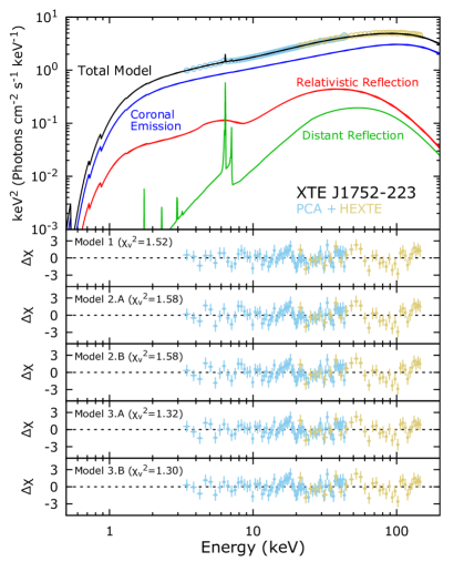
The results from these five fits are summarized in Table 2, and the the model components obtained for Model 1 (which are very similar in the other fits), together with the residuals of the five models are shown in Figure 4. The fit statistics are acceptable in all the fits, in particular if one considers the remarkably large number of source counts in these observations (about 100 million overall), and the very low systematics (0.1%). Model 1 appears to be slightly better than Model 2 based on the statistics, however, the improvement over the lamppost version is only marginal ($\Delta\chi^{2}=5-6$, with respect to Models 2.B–2.A, respectively). The inclusion of the extra Comptonization of the reflected component in Models 3 results in a much more significant improvement, with a decrease of $\Delta\chi^{2}=26$ with respect to Models 2, with the addition of only one extra free parameter. The differences, although statistically significant, are difficult to discern by eye from the residuals shown in the lower panels of Figure 4. This is once again a consequence of the very high signal-to-noise ratio of this dataset.

Figure 5.— Probability contours derived from the MCMC analysis of the fits using free emissivity index (Model 1, left panels), and with the lamppost geometry with free inner-radius (Model 2.A, right panels). A selection of important parameters is shown: inner radius, inclination, emissivity index, and coronal height. The strongest degeneracies are seeing among parameters in Model 1.

Given the complexity of the reflection models adopted here, the statistical analysis of all the fits, including the uncertainties of the parameters quoted in Table 2, was achieved by implementing a Markov Chain Monte-Carlo (MCMC) algorithm. Specifically, we used the emcee-hammer Python package (Foreman-Mackey et al., 2013), which allows efficient exploration of complex parameter spaces in determining posterior probability distributions. Each MCMC run consisted of 100–128 walkers (distinct chains), which was run until convergence was reached. Convergence was assessed by requiring that for each parameter at least 12 autocorrelation lengths were traversed by the average walker. The first third of the run was then discarded as burn-in phase.

Figure 6.— Probability contours derived from the MCMC analysis of the fits using free emissivity index (Model 1, left panels), and with the lamppost geometry with free inner-radius (Model 2.A, right panels). A selection of important parameters is shown: photon index, coronal height, emissivity index, reflection fraction, Fe abundance, and the normalization of the relativistic reflection component. Most of these contours are consistent with each other, and no strong degeneracies are observed.

4. Discussion

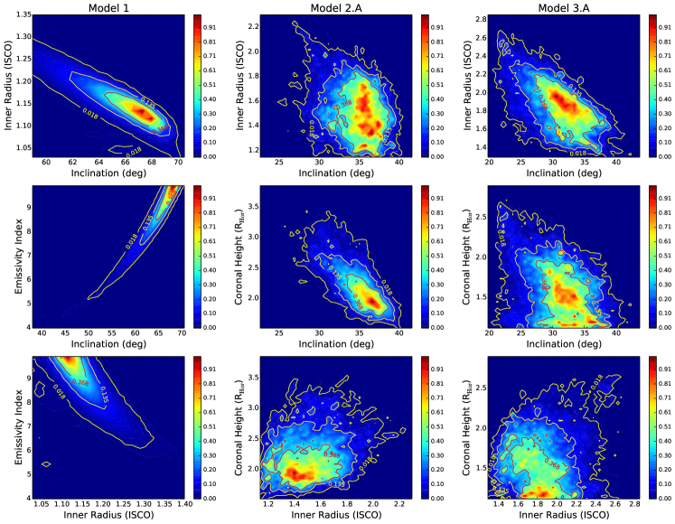
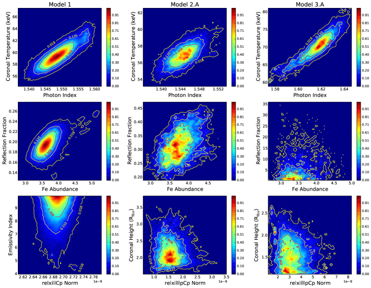
In Figures 5 and 6 we show the contour maps derived via MCMC analysis for a set of the most relevant physical parameters. For each map we also show the 1-, 2-, and 3-$\sigma$ confidence contours. These maps illustrate how well these parameters are constrained in each fit, and the level of degeneracy between parameters. In particular, we can see clear correlations between the inner radius, inclination, and the emissivity index (in the case of Model 1), or the height of the corona (in the case of Model 2.A). These correlations appear to be much stronger for Model 1 than for Model 2.A and Model 3.A (Figure 5). We also observe the expected correlation between the coronal temperature and the photon index in both fits, while other important parameters such as reflection fraction and Fe abundance, or the emissivity/coronal height and the normalization, show little dependence on each other (Figure 6).

Despite the fact that Model 1 yields a slightly better fit than Model 2.A, it does not necessarily provide the best physical interpretation of the data. In Model 1, the relativistic reflection component is assumed to follow an emissivity profile in the form of a power law in the radial coordinate. In other words, the net reflected emission $F_{\mathrm{ref}}$ follows $F_{\mathrm{ref}}\propto r^{-q}$. As noted in the progression of models of Section 3.1, the fit with Model 1 requires the emissivity index to be very large, essentially pegging the parameter at its maximum value of 10. At 90% confidence, a lower limit is found at $>7.2$.

The very steep emissivity found with Model 1 suggests an extreme relativistic scenario where the illumination is compact and concentrated at the central regions. This motivated the application of lamppost geometry in Models 2 and 3, where the relxillCp component is replaced by relxilllpCp.

In Models 2.A & 3.A the spin is also fixed at the Thorne limit, while $R_{\mathrm{in}}$ is let free to vary. Thus, these fits can be directly compared to the results from Model 1. Between Model 2.A and Model 1, all parameters are consistent within their uncertainties, with two exceptions: The reflection fraction in Model 2.A is roughly 1.5 times the value found with Model 1. The differences are more pronounced when comparing to Model 3.A. In the Model 3 variants, the inclusion of coronal Comptonization results in a reflection fraction an order of magnitude larger than in Model 2 or Model 1. (In fact, $R_{f}$ is distributed approximately log-normal, with a 99% lower limit of $>0.3$ for Model 3.A.) Because Comptonization hardens the reflection output, the intrinsic emission is found to be significantly softer $\Delta\Gamma\approx 0.07$ and the electron temperature is likewise higher ($\Delta kT_{e}\approx 12$ keV).

Most importantly, Models 2 and 3 strongly disagree with Model 1 on the inclination of the system: the best-fit value for Model 1 is $67^{+2}_{-8}$ deg, while for Model 2.A and  3.A the values are $35^{+3}_{-5}$ deg and $31\pm 6$ deg, respectively. Meanwhile, Miller-Jones et al. (2011) found an upper limit of the inclination of $i<49$ deg based on radio observations of the jet when the source was transitioning from the hard to the soft state. This upper limit thus formally excludes the large inclination value from Model 1. It is possible that the extreme relativistic effects are forcing the fit in Model 1 to increase the emissivity index to unphysical values. A very large value of the emissivity index will produce two effects. Firstly, it increases the blurring of the reflection spectrum, broadening the Fe K line. Secondly, it shifts photons to lower energies. Broadening of the Fe K line is likely to be required, but the extreme value of $q$ redshifts the line outside of the observed range. The model then compensates by increasing the inclination, which shifts the line back to higher energies. We notice that a similar effect of the lamppost model bringing the inclination to more reasonable levels was previously reported by Tomsick et al. (2014) in their analysis of Cyg X-1 data. The large inclination of Model 1 is interpreted as the result of this tension between the model parameters. We therefore disregard Model 1 and focus only on the application of the lamppost model, which we then use to derive all the physical parameters for the black hole system XTE J1752–223.

The results of the fits with all models (Table 2) indicate that the primary source of X-ray photons is located very close to the black hole, specifically at $h\lesssim 2~{}R_{\mathrm{Hor}}$, where $R_{\mathrm{Hor}}=1.063$ $R_{g}$ is the event horizon radius for a black hole rotating at the Thorne limit. This again supports the idea of extreme illumination of the inner regions of the accretion disk, causing a relativistically broadened reflection spectrum. For these parameters, we estimate that $\gtrsim 27\%$ of the photons emitted by the primary source will fall into the black hole without reaching the accretion disk. Furthermore, the lamppost model has the capability of predicting a reflection fraction by assuming the point-source lamppost emits isotropically in its rest frame. The corresponding reflection fraction for its height is $R_{\mathrm{f}}\gtrsim 5$, whereas the best fits with Models 2.A and 2.B find $0.30^{+0.10}_{-0.07}$ and $0.20^{+0.07}_{-0.11}$, respectively. This large difference is reconciled with the inclusion of Comptonization with Model 3. Similar results were found between these classes of models in the case of GX 339–4 (García et al., 2015b; Steiner et al., 2017). This difference is because the coronal scattering dilutes reflection’s apparent strength (e.g.; Steiner et al., 2016), so that larger $R_{\mathrm{f}}$ is required to fit the data.

Figures 5 and 6 show that the correlations between coronal height, inner disk radius and inclination in Model 3.A are mostly consistent with those of Model 2.A, aside from the differences described above for $\Gamma$ and $kT_{e}$. For Models 3, assuming a uniform-density corona, its optical depth is given by $f_{\mathrm{sc}}=1-\exp(-\tau)$, and we correspondingly find $\tau=1.8^{+0.1}_{-0.5}$ and $\tau=1.7^{+0.2}_{-0.4}$ for Models 3.A and 3.B, respectively. Comparison with Titarchuk (1994) shows that this temperature and optical depth are well-matched to the fitted $\Gamma$ under the assumption of a compact spherical geometry for the corona. Models 3.A and 3.B give statistically indistinguishable values of the inner disk radius and spin respectively compared to Models 2.A and 2.B, but a significant improvement in the fit quality ($\Delta\chi^{2}/\Delta\nu\approx 26/1$).

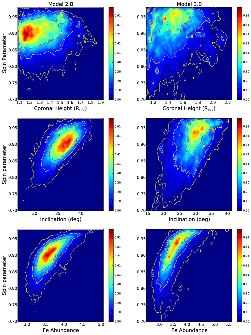
In all model variants we find that the inner-disk must be very close to the ISCO, leaving vanishing room for the possibility of disk truncation. Accordingly, the black hole spin must be quite high. The fits (Model 2.B: $a_{*}=$$0.92^{+0.05}_{-0.07}$, Model 3.B: $a_{*}=$ $0.95^{+0.04}_{-0.13}$) are actually lower limits, as the presence of any truncation effect would result in a higher spin. Figure 7 shows the contour maps for the spin in Models 2.B and 3.B versus three other important parameters: the coronal height, the inclination, and the iron abundance. While some correlations can be seen among these parameters, it is clear that under the assumption that the disk reaches the ISCO, spin is very well constrained. Perhaps the most obvious degeneracy is observed between the spin and the Fe abundance, which is a correlation expected and previously reported in fitting reflection models (e.g.; Reynolds et al., 2012; García et al., 2015b).

Figure 7.— Contour plots for the spin parameter as a function of the coronal height, the inclination, and the Fe abundance, as obtained from the MCMC analysis with Model 2.B and Model 3.B.

The high spin value obtained with Model 2.B and Model 3.B disagrees with that from Reis et al. (2011), who have previously reported an intermediate spin of $a_{*}=0.52\pm 0.11$, the only other determination obtained through reflection spectroscopy. We now discuss some of the possible reasons for this discrepancy. The two observations analyzed by Reis et al. (2011) were taken during the decay of the outburst, one in the intermediate state (with Suzaku) and another in the low hard state (with XMM-Newton). The data were modeled with the reflection model REFBHB (Ross & Fabian, 2007). Although this model self-consistently includes the thermal disk emission, it also assumes a single-temperature accretion disk and implements outdated atomic data. More importantly, the iron abundance is fixed at the solar value. As described Section 6.3 of García et al. (2015b) (as well as in Wang-Ji et al., 2018), the Fe K emission profile from a truncated disk with Solar abundances looks very similar to that from a disk that extends down to the ISCO but for which the Fe abundance is enhanced. These two situations can only be clearly differentiated in the $\sim$10–20 keV range (see Figure 12 in García et al., 2015b), which is coincidentally the region not covered by the data analyzed in Reis et al. (2011).

Another important aspect of the analysis presented by Reis et al. (2011) is that due to the high count rate of the source, the XMM-Newton observation was taken in the timing mode. We have found, through the analysis of XTE J1752–223 and other sources, serious discrepancies between the XMM-Newton data taken in this mode and simultaneous data taken by other instruments such as the PCA in RXTE. These discrepancies are likely due to calibration uncertainties in the XMM-Newton timing mode This discrepancy has also been noticed in the observations of the bright hard state of GX 339–4 (Basak & Zdziarski, 2015). Despite the fact that Reis et al. (2011) also included one Suzaku observation in their work, it is likely that the XMM-Newton data is dominating the results of their fits, since the count rate of the XMM-Newton spectrum is between 1 and 2 orders of magnitude larger in the Fe K band (e.g.; see their Figure 6).

In general, the results from our fits to XTE J1752–223 resemble those found previously for GX 339–4 in its bright hard state (García et al., 2015b; Steiner et al., 2017; Wang-Ji et al., 2018). We find an accretion disk approaching very close to the ISCO, with a large Fe abundance with respect to the Solar value, a rapidly rotating black hole, and strong supporting evidence for the importance of accounting for Comptonization of the reflection emission.

5. Summary and Conclusions

We have presented an analysis of the bright hard state of the black hole binary system XTE J1752–223 during its 2009 outburst observed by RXTE. During the rise of the outburst this source was observed in a particularly stable hard state lasting roughly one month. By combining observations taken during this period of time, we have been able to obtain an spectrum with remarkable statistical weight: a total of $\sim 100$ million source counts between PCU-2 and HEXTE bands. We find the relxill models are very successful in describing these data through a combination of a thermal Comptonization continuum, unblurred distant reflection, and relativistically blurred reflection components. Despite the extreme statistical quality of this dataset, and the low systematics included—0.1% per the use of our pcacorr tool—the fit statistics are satisfactory ($\chi_{\nu}^{2}\sim 1.3-1.6$). This is, to our knowledge, the highest signal-to-noise X-ray reflection spectrum published to date.

We found that the data can be almost equally well described with either an extended coronal model or a lamppost geometry. In the former, the required emissivity index is extreme, which suggests a compact emitting region for the primary source of photons. When the lamppost geometry is implemented, all parameters are consistent with the coronal model with the exception of the inclination and reflection fraction. Inclination changes most dramatically, from $\sim 67$ deg for the coronal model to $\sim 30-35$ deg for the lamppost models. The lamppost results agrees with the upper limit of $i<49$ deg reported by Miller-Jones et al. (2011) from radio jet observations, and it is thus preferred.

The modeling of the reflection spectrum of XTE J1752–223 shares several similarities with the parameters found previously for the bright hard-state in GX 339–4: a rapidly rotating black hole with an accretion disk extending very close-in with super-solar iron abundance. Likewise, without accounting for Comptonization of the reflection emission, the reflection fraction is found to be much lower than that predicted self-consistently by the lamppost geometry. While the high spin result contradicts the intermediate spin values derived by Reis et al. (2011), we argue that this discrepancy is likely due to calibration uncertainties in their data, or possibly due to the lack of coverage in the 10–30 keV region, a spectral band that is crucial to disentangle high from low spin models, particularly if Solar Fe abundance is assumed.

Just as in the case of GX 339–4, we found that the reflection spectrum of XTE J1752–223 is largely affected by relativistic smearing, which requires the inner accretion disk to be located very close to the black hole. This result would then suggest that at the bright-end of the hard state, the accretion disk in these systems approaches close to, or reaches the ISCO, before their transition to the soft state. The fact that XTE J1752–223 spent an entire month in the bright hard state, without showing any significant changes in luminosity or spectral hardness, suggests that the system must have been in a very stable configuration, which is plausible if the disk has reached the ISCO. If this interpretation is correct, it could possibly mean that the transition to the soft state is then triggered not by a change in the disk’s geometry, but rather by a different physical process. A sudden change in the accretion rate could presumably induce such a change, increasing the temperature of the accretion disk and pushing the system into the soft state. The present discussion is merely speculative at this point, which is why intense monitoring campaigns of this and similar sources are highly motivated to better understand their physical nature.

References

- Arnaud (1996) Arnaud, K. A. 1996, in Astronomical Society of the Pacific Conference Series, Vol. 101, Astronomical Data Analysis Software and Systems V, ed. G. H. Jacoby & J. Barnes, 17
- Basak & Zdziarski (2015) Basak, R., & Zdziarski, A. A. 2015, ArXiv e-prints
- Brocksopp et al. (2013) Brocksopp, C., Corbel, S., Tzioumis, A., Broderick, J. W., Rodriguez, J., Yang, J., Fender, R. P., & Paragi, Z. 2013, MNRAS, 432, 931
- Brocksopp et al. (2010) Brocksopp, C., Corbel, S., Tzioumis, T., Fender, R., & Coriat, M. 2010, The Astronomer’s Telegram, 2400
- Dauser et al. (2014) Dauser, T., García, J., Parker, M. L., Fabian, A. C., & Wilms, J. 2014, MNRAS, 444, L100
- Dauser et al. (2013) Dauser, T., Garcia, J., Wilms, J., Böck, M., Brenneman, L. W., Falanga, M., Fukumura, K., & Reynolds, C. S. 2013, MNRAS, 430, 1694
- Dauser et al. (2010) Dauser, T., Wilms, J., Reynolds, C. S., & Brenneman, L. W. 2010, MNRAS, 409, 1534
- Done et al. (2007) Done, C., Gierliński, M., & Kubota, A. 2007, A&A Rev., 15, 1
- Dove et al. (1997) Dove, J. B., Wilms, J., Maisack, M., & Begelman, M. C. 1997, ApJ, 487, 759
- Fabian (2012) Fabian, A. C. 2012, ARA&A, 50, 455
- Fabian et al. (2017) Fabian, A. C., Lohfink, A., Belmont, R., Malzac, J., & Coppi, P. 2017, MNRAS, 467, 2566
- Fabian et al. (2015) Fabian, A. C., Lohfink, A., Kara, E., Parker, M. L., Vasudevan, R., & Reynolds, C. S. 2015, MNRAS, 451, 4375
- Foreman-Mackey et al. (2013) Foreman-Mackey, D., Hogg, D. W., Lang, D., & Goodman, J. 2013, PASP, 125, 306
- García et al. (2013) García, J., Dauser, T., Reynolds, C. S., Kallman, T. R., McClintock, J. E., Wilms, J., & Eikmann, W. 2013, ApJ, 768, 146
- García & Kallman (2010) García, J., & Kallman, T. R. 2010, ApJ, 718, 695
- García et al. (2011) García, J., Kallman, T. R., & Mushotzky, R. F. 2011, ApJ, 731, 131
- García et al. (2014a) García, J., et al. 2014a, ApJ, 782, 76
- García & Dauser (2018) García, J. A., & Dauser, T. 2018, In Preparation
- García et al. (2015a) García, J. A., Dauser, T., Steiner, J. F., McClintock, J. E., Keck, M. L., & Wilms, J. 2015a, ApJ, 808, L37
- García et al. (2016) García, J. A., Grinberg, V., Steiner, J. F., McClintock, J. E., Pottschmidt, K., & Rothschild, R. E. 2016, ApJ, 819, 76
- García et al. (2014b) García, J. A., McClintock, J. E., Steiner, J. F., Remillard, R. A., & Grinberg, V. 2014b, ApJ, 794, 73
- García et al. (2015b) García, J. A., Steiner, J. F., McClintock, J. E., Remillard, R. A., Grinberg, V., & Dauser, T. 2015b, ApJ, 813, 84
- Grinberg et al. (2013) Grinberg, V., et al. 2013, A&A, 554, A88
- Haardt (1993) Haardt, F. 1993, ApJ, 413, 680
- Homan & Belloni (2005) Homan, J., & Belloni, T. 2005, Ap&SS, 300, 107
- Jahoda et al. (2006) Jahoda, K., Markwardt, C. B., Radeva, Y., Rots, A. H., Stark, M. J., Swank, J. H., Strohmayer, T. E., & Zhang, W. 2006, ApJS, 163, 401
- Madau & Fragos (2017) Madau, P., & Fragos, T. 2017, ApJ, 840, 39
- Markoff et al. (2005) Markoff, S., Nowak, M. A., & Wilms, J. 2005, ApJ, 635, 1203
- Markwardt et al. (2009a) Markwardt, C. B., Barthelmy, S. D., Evans, P. A., & Swank, J. H. 2009a, The Astronomer’s Telegram, 2261
- Markwardt et al. (2009b) Markwardt, C. B., et al. 2009b, The Astronomer’s Telegram, 2258
- Matt et al. (1992) Matt, G., Perola, G. C., Piro, L., & Stella, L. 1992, A&A, 257, 63
- McClintock & Remillard (2006) McClintock, J. E., & Remillard, R. A. 2006, Black hole binaries (Cambridge University Press, London), 157–213
- Miller-Jones et al. (2011) Miller-Jones, J. C. A., Jonker, P. G., Ratti, E. M., Torres, M. A. P., Brocksopp, C., Yang, J., & Morrell, N. I. 2011, MNRAS, 415, 306
- Mirabel & Rodríguez (1999) Mirabel, I. F., & Rodríguez, L. F. 1999, ARA&A, 37, 409
- Nakahira et al. (2009) Nakahira, S., et al. 2009, The Astronomer’s Telegram, 2259
- Peris et al. (2016) Peris, C. S., Remillard, R. A., Steiner, J. F., Vrtilek, S. D., Varnière, P., Rodriguez, J., & Pooley, G. 2016, ApJ, 822, 60
- Reis et al. (2011) Reis, R. C., et al. 2011, MNRAS, 410, 2497
- Remillard & ASM Team at MIT (2009) Remillard, R. A., & ASM Team at MIT. 2009, The Astronomer’s Telegram, 2265
- Remillard & McClintock (2006) Remillard, R. A., & McClintock, J. E. 2006, ARA&A, 44, 49
- Reynolds et al. (2012) Reynolds, C. S., Brenneman, L. W., Lohfink, A. M., Trippe, M. L., Miller, J. M., Fabian, A. C., & Nowak, M. A. 2012, ApJ, 755, 88
- Ross & Fabian (2007) Ross, R. R., & Fabian, A. C. 2007, MNRAS, 381, 1697
- Rothschild et al. (1998) Rothschild, R. E., et al. 1998, ApJ, 496, 538
- Shaposhnikov (2010) Shaposhnikov, N. 2010, The Astronomer’s Telegram, 2391
- Shaposhnikov et al. (2010) Shaposhnikov, N., Markwardt, C., Swank, J., & Krimm, H. 2010, ApJ, 723, 1817
- Shaposhnikov et al. (2009) Shaposhnikov, N., Markwardt, C. B., & Swank, J. H. 2009, The Astronomer’s Telegram, 2269
- Steiner et al. (2017) Steiner, J. F., García, J. A., Eikmann, W., McClintock, J. E., Brenneman, L. W., Dauser, T., & Fabian, A. C. 2017, ApJ, 836, 119
- Steiner et al. (2010) Steiner, J. F., McClintock, J. E., Remillard, R. A., Gou, L., Yamada, S., & Narayan, R. 2010, ApJ, 718, L117
- Steiner et al. (2016) Steiner, J. F., Remillard, R. A., García, J. A., & McClintock, J. E. 2016, ApJ, 829, L22
- Thorne (1974) Thorne, K. S. 1974, ApJ, 191, 507
- Titarchuk (1994) Titarchuk, L. 1994, ApJ, 434, 570
- Tomsick et al. (2014) Tomsick, J. A., et al. 2014, ApJ, 780, 78
- Toor & Seward (1974) Toor, A., & Seward, F. D. 1974, AJ, 79, 995
- Verner et al. (1996) Verner, D. A., Ferland, G. J., Korista, K. T., & Yakovlev, D. G. 1996, ApJ, 465, 487
- Wang-Ji et al. (2018) Wang-Ji, J., et al. 2018, ApJ, 855, 61
- Wilms et al. (2000) Wilms, J., Allen, A., & McCray, R. 2000, ApJ, 542, 914
- Wilson-Hodge et al. (2011) Wilson-Hodge, C. A., et al. 2011, ApJ, 727, L40
- Yang et al. (2010) Yang, J., Brocksopp, C., Corbel, S., Paragi, Z., Tzioumis, T., & Fender, R. P. 2010, MNRAS, 409, L64
- Yang et al. (2011) Yang, J., Paragi, Z., Corbel, S., Gurvits, L. I., Campbell, R. M., & Brocksopp, C. 2011, MNRAS, 418, L25
- Zdziarski et al. (1996) Zdziarski, A. A., Johnson, W. N., & Magdziarz, P. 1996, MNRAS, 283, 193
- Zdziarski et al. (2003) Zdziarski, A. A., Lubiński, P., Gilfanov, M., & Revnivtsev, M. 2003, MNRAS, 342, 355
- Życki et al. (1999) Życki, P. T., Done, C., & Smith, D. A. 1999, MNRAS, 309, 561