Bosonic Gaussian states from conformal field theory

Abstract

We study nonchiral wave functions for systems with continuous spins obtained from the conformal field theory (CFT) of a free, massless boson. In contrast to the case of discrete spins, these can be treated as bosonic Gaussian states, which allows us to efficiently compute correlations and entanglement properties both in one (1D) and in two spatial dimensions (2D). In 1D, the computed entanglement entropy and spectra are in agreement with the underlying CFT. Furthermore, we construct a 1D parent Hamiltonian with a low-energy spectrum corresponding to that of a free, massless boson. In 2D, we find edge excitations in the entanglement spectrum, although the states do not have intrinsic topological order, as revealed by a determination of the topological entanglement entropy.

I Introduction

The main challenge in the theoretical study of many-body systems is given by the exponential scaling of the Hilbert space with the system size. Since exact diagonalization techniques are limited to small systems, studying simple models is essential for understanding intricate many-body phenomena. One way to build such models is to define them through Hamiltonians. A different approach is based on wave functions representing model states in a variational sense. The most prominent example is given by Laughlin’s wave function Laughlin (1983) and its generalizations Haldane (1983); Halperin (1984); Moore and Read (1991). These provide good variational descriptions of electrons in a fractional quantum Hall Tsui et al. (1982) (FQH) phase and thus represent paradigmatic models of systems exhibiting topological order Wen (1990a, 2016). Laughlin’s wave function is the two-dimensional (2D) analog of the ground state belonging to the one-dimensional (1D) Calogero-Sutherland model Calogero (1969, 1971); Sutherland (1971a, b).

In the past years, there has been an increased interest in lattice models exhibiting topological properties and in implementing these with systems consisting of ultracold atoms, see for example Refs. Sørensen et al., 2005; Hafezi et al., 2007; Cooper and Dalibard, 2013; Yao et al., 2013; Goldman et al., 2016. An advantage of this approach is that the interaction strength can be tuned experimentally Bloch et al. (2008). Thus, strongly interacting regimes can be achieved where extraordinary many-body effects are expected to be more pronounced and occur at higher temperatures. Recent experimental achievements in this field include the implementation of the Hofstadter model Aidelsburger et al. (2013); Miyake et al. (2013) and the simulation of a four-dimensional FQH effect Lohse et al. (2018); Zilberberg et al. (2018). Important theoretical models on lattices are given by the chiral spin liquid Kalmeyer and Laughlin (1987, 1989), which is the lattice version of Laughlin’s wave function, its nonabelian generalization Greiter and Thomale (2009), and also the Haldane-Shastry model Haldane (1988); Shastry (1988), which is the lattice analog of the Calogero-Sutherland model. Recently, an exact parent Hamiltonian of the chiral spin liquid was found Thomale et al. (2009); Nielsen et al. (2012), which led to a proposal for an implementation with ultracold atoms Nielsen et al. (2013).

In a seminal paper, Moore and Read Moore and Read (1991) showed that Laughlin’s and other FQH wave functions can be constructed systematically using conformal field theory (CFT) in 1(+1) dimension. In this approach, a FQH wave function is defined as a chiral CFT correlator. Since CFT is associated with the gapless boundary excitations Halperin (1982); Wen (1990b, c, 1991, 1992) of a quantum Hall system, this is an example of a bulk-edge correspondence Dubail et al. (2012). The description of a FQH state in terms of CFT thus establishes a connection between the topological order of the state and its edge theory Witten (1989); Dubail et al. (2012). The idea of building model states from CFT was later also applied to lattice systems with discrete spin or fermionic degrees of freedom Cirac and Sierra (2010). In 1D, ground states of Haldane-Shastry spin chains were obtained in this way Cirac and Sierra (2010); Nielsen et al. (2011), while these states describe quantum Hall lattice systems in 2D. A wave function of free fermions occurs as a special case having a vanishing topological entanglement entropy Nielsen et al. (2012). It is an example of a chiral state with non-intrinsic topological order and represents a lattice version of the integer quantum Hall Klitzing et al. (1980) effect. Other 2D lattice states obtained from CFT were shown to exhibit intrinsic topological order and describe FQH phases Nielsen et al. (2012); Tu et al. (2014); Glasser et al. (2016).

Given the construction of model states in terms of CFT, it is natural to ask how their physical properties are related to the CFT they are constructed from. For states in 1D, it was shown that correlations and entanglement entropies are in accordance with the CFT expectation Tu et al. (2014). In 2D, CFT is associated with the gapless edge of FQH systems. As shown in Ref. Dubail et al., 2012 for the case FQH states with continuous spatial degrees of freedom, the assumption of exponentially decaying bulk correlations implies that the edge correlations are determined by CFT. Except in special cases like that of free fermions Nielsen et al. (2012), the determination of correlations and entanglement entropies of states defined through CFT requires the use of Monte Carlo for large systems, where exact methods fail. Recently Herwerth et al. (2017), we made an approximation for correlations in a class of abelian FQH lattice states and the corresponding 1D wave functions. This approximation corresponds to replacing the discrete spin-$\frac{1}{2}$ degrees of freedom by continuous spins, which makes it possible to obtain exact results for large systems. We found good quantitative agreement between the actual correlations and the approximation in a certain parameter range. In 2D, the approximation has polynomially decaying edge correlations and exponentially decaying bulk correlations.

In this paper, we adopt Moore and Read’s approach and define a class of spin states on lattices from the CFT of a massless, free boson. Opposed to earlier studies on lattices, we consider the case of continuous spins $s\in\mathbb{R}$. On the one hand, this implies that these states have the correlations that we used earlier Herwerth et al. (2017) to approximate the spin-$\frac{1}{2}$ case. On the other hand, they represent another example of model states constructed from CFT, and the aim of this paper is to investigate and characterize them. The main motivation for studying the case of continuous spins is that the resulting wave functions are Gaussian. Opposed to the discrete case, their properties can thus be computed efficiently using the framework of bosonic Gaussian states. Following a new development of the past years Vidal et al. (2003); Calabrese and Cardy (2004); Kitaev and Preskill (2006); Levin and Wen (2006); Li and Haldane (2008), we use entanglement properties as the central tool to characterize the states and investigate their topological properties.

In 1D, the states are closely related to the CFT they are constructed from: We show that their entanglement entropies and low-lying momentum-space entanglement energies agree with those of a massless, free boson. We also construct a parent Hamiltonian in 1D with low-lying energies corresponding to that of the CFT. In 2D, we confirm that the states do not have intrinsic topological order since their topological entanglement entropy Levin and Wen (2006); Kitaev and Preskill (2006) vanishes as expected for Gaussian states. On the other hand, we observe low-lying states in the entanglement spectrum that are exponentially localized at the edge. The wave functions studied in this paper are constructed from the complete (chiral + antichiral) CFT and are thus real and nonchiral. This absence of chirality is similar to the quantum spin Hall effect Kane and Mele (2005a, b); Bernevig and Zhang (2006). We also comment on the corresponding chiral wave function, which is equivalent to the real case in 1D. For general lattices, however, the chiral state depends on the ordering of the lattice positions, which is in contrast to the real wave function. This could indicate that the chiral case does not fall under the framework of bosonic Gaussian states, and we leave this case open for future investigations.

This paper is structured as follows: Sec. II defines the states with continuous spins studied in this paper, shows how they can be represented as bosonic Gaussian states, and explains how we compute entanglement properties for them. We discuss results for a 1D system with periodic boundary conditions in Sec. III and for 2D systems on the cylinder in Sec. IV. Sec. V concludes this paper.

II Spin states from conformal field theory

This section defines states with a continuous spin as correlators of the free-boson CFT, represents them as bosonic Gaussian states, and explains how we compute entanglement properties.

II.1 Definition of states

We consider the CFT of a massless, free bosonic field $\varphi(z,\bar{z})$ for $z\in\mathbb{C}$. This theory has a series of conformal primary fields $:e^{is\varphi(z,\bar{z})}:$ for $s\in\mathbb{R}$, where the colons denote normal ordering. We define spin wave functions as the correlator of primary fields:

$$\psi_{\beta}(\bm{s})$$ (1)

$$\quad=e^{-\frac{1}{4}\left(\beta+\beta_{0}\right)\bm{s}^{2}}\langle:e^{\frac{i}{\sqrt{2}}s_{1}\varphi(z_{1},\bar{z}_{1})}:\dots:e^{\frac{i}{\sqrt{2}}s_{N}\varphi(z_{N},\bar{z}_{N})}:\rangle$$

$$\quad=e^{-\frac{1}{4}\left(\beta+\beta_{0}\right)\bm{s}^{2}}\delta\left(s_{1}+\dots+s_{N}\right)\prod_{m<n}\left|z_{m}-z_{n}\right|^{s_{m}s_{n}},$$

where $z_{j}$ for $j\in\{1,\dots,N\}$ defines a lattice of positions in the complex plane, $\bm{s}\in\mathbb{R}^{N}$ is a vector of $N$ continuous spin variables, $\delta$ is the Dirac delta function originating from the charge neutrality condition, and $\beta>0$ is a real parameter. We define the real number $\beta_{0}$ through a normalizability criterion and introduce $\beta_{0}$ separately from $\beta$ for convenience so that $\beta$ is always positive, cf. Sec. II.3 below. The parametric dependence of $\psi_{\beta}(\bm{s})$ on the lattice positions $z_{j}$ is suppressed for simplicity of notation.

The prefactor $e^{-\frac{1}{4}\left(\beta+\beta_{0}\right)\bm{s}^{2}}$ in Eq. (1) corresponds to a rescaling $(z_{j},\bar{z}_{j})\to(\lambda z_{j},\lambda\bar{z}_{j})$ with $\lambda>0$, under which the correlation function of primary fields $:e^{\frac{i}{\sqrt{2}}s_{j}\varphi(z_{j},\bar{z}_{j})}:$ changes by a factor $\lambda^{-\frac{1}{2}\bm{s}^{2}}$. Comparing to the form of the wave function of Eq. (1), we have $\beta+\beta_{0}=2\ln\lambda$ in terms of the scale parameter $\lambda$ of the lattice. In the definition of $\psi_{\beta}(\bm{s})$, we do not include an additional parameter in the exponent of the vertex operators as in the case of discrete spins Cirac and Sierra (2010). The reason is that such a parameter can be removed by a rescaling of the continuous spins $s_{j}\in\mathbb{R}$.

In a previous study Herwerth et al. (2017), we considered continuous-spin approximations for correlations of spin-$\frac{1}{2}$ states obtained from CFT. The wave functions $\psi_{\beta}(\bm{s})$ have the same correlations as the approximation that was made in Ref. Herwerth et al., 2017, cf. Appendix D for details.

In this work, we focus on the case of a real wave function $\psi_{\beta}(\bm{s})$ defined through operators $:e^{\frac{i}{\sqrt{2}}s_{j}\varphi(z_{j},\bar{z}_{j})}:$ with chiral and antichiral components. We comment on the corresponding chiral wave function in Appendix E, where we also show that $\psi_{\beta}(\bm{s})$ is equivalent to the chiral case for a uniform 1D lattice with periodic boundary conditions.

II.2 Representation as a Gaussian state

We now represent $\psi_{\beta}(\bm{s})$ as a bosonic Gaussian state, which implies that its properties can be computed efficiently for large systems. To this end, we replace the delta function $\delta(s_{1}+\dots+s_{N})$ in $\psi_{\beta}(\bm{s})$ by a Gaussian of width proportional to $\sqrt{\epsilon}$ for $\epsilon>0$. This leads to the wave function

$$\psi_{\beta,\epsilon}(\bm{s}) =e^{-\frac{1}{2}\bm{s}^{t}(\frac{1}{2\epsilon}\bm{e}\bm{e}^{t}+X_{\beta})\bm{s}},$$ (2)

where

$$\left(X_{\beta}\right)_{mn} =\frac{1}{2}\left(\beta+\beta_{0}\right)\delta_{mn}+X_{mn},$$ (3)

$$X_{mn} =-\ln\left(|z_{m}-z_{n}|+\delta_{mn}\right),$$ (4)

and $\bm{e}=(1,\dots,1)^{t}$ is the vector with all entries being equal to one. Then,

$$\psi_{\beta}(\bm{s}) =\lim_{\epsilon\to 0}\frac{1}{2\sqrt{\pi\epsilon}}\psi_{\beta,\epsilon}(\bm{s}).$$ (5)

Defining

$$X_{\beta,\epsilon} =\frac{1}{2\epsilon}\bm{e}\bm{e}^{t}+X_{\beta}\equiv\frac{1}{2\epsilon}\bm{e}\bm{e}^{t}+\frac{1}{2}\left(\beta+\beta_{0}\right)\mathbb{I}+X,$$ (6)

where $\mathbb{I}$ is the $N\times N$ identity matrix, $\psi_{\beta,\epsilon}(\bm{s})$ assumes the standard form of a pure, bosonic Gaussian state (cf. Appendix A):

$$\psi_{\beta,\epsilon}(\bm{s}) =e^{-\frac{1}{2}\bm{s}^{t}X_{\beta,\epsilon}\bm{s}}.$$ (7)

II.3 Definition of $\beta_{0}$

We define $\beta_{0}$ by requiring that $\psi_{\beta,\epsilon}(\bm{s})$ is normalizable for all $\beta>0$. According to Eq. (3), we have

$$\beta_{0}=-2\min\{\lambda_{\epsilon}^{(1)},\dots,\lambda_{\epsilon}^{(N)}\},$$ (8)

where $\{\lambda_{\epsilon}^{(1)},\dots,\lambda_{\epsilon}^{(N)}\}$ are the eigenvalues of $\frac{1}{2\epsilon}\bm{e}\bm{e}^{t}+X$.

In the limit $\epsilon\to 0$, the matrix $\frac{1}{2\epsilon}\bm{e}\bm{e}^{t}+X$ becomes divergent, and we determine $\{\lambda_{\epsilon}^{(1)},\dots,\lambda_{\epsilon}^{(N)}\}$ as the inverse eigenvalues of

$$\left[\frac{1}{2\epsilon}\bm{e}\bm{e}^{t}+X\right]^{-1} =X^{-1}-\frac{X^{-1}\bm{e}\bm{e}^{t}X^{-1}}{2\epsilon+\bm{e}^{t}X^{-1}\bm{e}},$$ (9)

where we used a general formula for the inverse of a matrix that is changed by a term of rank one Bartlett (1951).

II.4 Entanglement properties

The representation of $\psi_{\beta}(\bm{s})$ as a Gaussian state allows us to efficiently compute its entanglement properties under partition of the system into parts $A$ and $B$, cf. Appendix B for details.

In summary, we find that the Rényi entanglement entropies $S_{a}(A)$ of order $a$ are given by

$$S_{a}(A) =-\frac{1}{2}\ln\epsilon+S_{a}^{\prime}(A)+\mathcal{O}(\epsilon),$$ (10)

where $S_{a}^{\prime}(A)$ is independent of $\epsilon$. The divergence in $S_{a}(A)$ for $\epsilon\to 0$ is a consequence of the delta function $\delta(s_{1}+\dots+s_{N})$ in $\psi_{\beta}(\bm{s})$. By subtracting it, we obtain the finite entropies $S_{a}^{\prime}(A)$. The entanglement Hamiltonian can be brought into the diagonal form $\sum_{j=1}^{|A|}\tilde{\omega}_{j}b^{\dagger}_{j}b_{j}$ in a suitable basis of annihilation and creation operators $b_{j}$ and $b_{j}^{\dagger}$. The single-particle energies $\tilde{\omega}_{j}$ determine the entanglement spectrum.

II.5 States on the cylinder

For the rest of this paper, we study a system on a cylinder with a square lattice of $N_{x}$ sites in the open and $N_{y}$ sites in the periodic direction:

$$w_{m} \equiv w_{m_{x}m_{y}}=\frac{2\pi}{N_{y}}\left(m_{x}+im_{y}\right),$$ (11)

where $m_{x}$ is the $x$ and $m_{y}$ the $y$ component of the index $m$ [$m=(m_{x}-1)N_{y}+m_{y}$], and we identify $w_{m_{x}m_{y}}$ with $w_{m_{x},m_{y}+N_{y}}$. This includes a uniform lattice in 1D with periodic boundary conditions as the special case $N_{x}=1$.

The wave function $\psi_{\beta}(\bm{s})$ was defined for positions $z_{j}$ in the complex plane in Eq. (1). For positions $w_{j}$ on the cylinder, we use the map $z_{j}=e^{w_{j}}$ from the cylinder to the plane and define the wave function by evaluating the CFT correlator on the cylinder:

$$\psi_{\beta}(\bm{s})$$ (12)

$$\quad=e^{-\frac{1}{4}\left(\beta+\beta_{0}\right)\bm{s}^{2}}\langle:e^{\frac{i}{\sqrt{2}}s_{1}\varphi(w_{1},\bar{w}_{1})}:\dots:e^{\frac{i}{\sqrt{2}}s_{N}\varphi(w_{N},\bar{w}_{N})}:\rangle$$

$$\quad=e^{-\frac{1}{4}\left(\beta+\beta_{0}\right)\bm{s}^{2}}\delta\left(s_{1}+\dots+s_{N}\right)$$

$$\quad\quad\times\prod_{m<n}\left|2\sinh\left(\frac{1}{2}(w_{m}-w_{n})\right)\right|^{s_{m}s_{n}},$$

where we used Eq. (1) and the transformation rule for primary fields Di Francesco et al. (1997) under $z_{j}=e^{w_{j}}$. The definition of $\psi_{\beta,\epsilon}(\bm{s})$ introduced in Sec. II.2 changes accordingly on the cylinder.

III Properties of states in 1D

In this section, we study properties of $\psi_{\beta}(\bm{s})$ for a 1D system with periodic boundary conditions. We show that the correlations, entanglement properties, and a parent Hamiltonian exhibit signatures of the underlying CFT of a free, massless boson.

III.1 Correlations

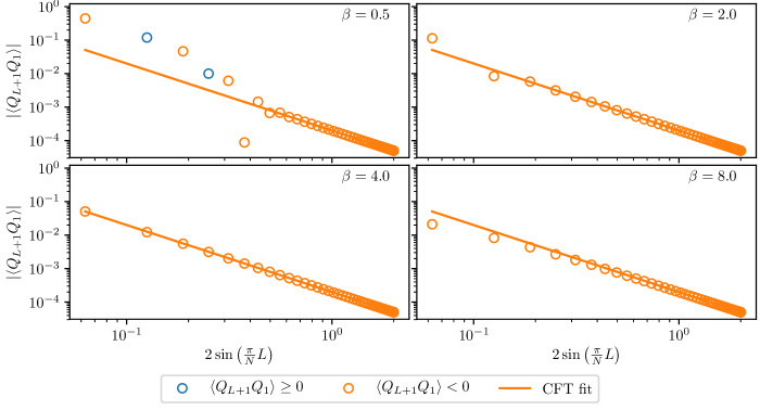
Figure 1: (Color online) Spin-Spin correlations $\langle Q_{L+1}Q_{1}\rangle$ in $\psi_{\beta}(\bm{s})$ in 1D with periodic boundary conditions for $N=100$ sites. The operator $Q_{m}$ is defined as $(Q_{m}\psi_{\beta})(\bm{s})=s_{m}\psi_{\beta}(\bm{s})$. The long-range decay is consistent with the CFT expectation of an algebraic decay with a power of $-2$. The fit was done for the 10 data points with the largest value of $L$.

A plot of spin-spin correlations in $\psi_{\beta}(\bm{s})$ and a fit to the CFT expectation are shown in Fig. 1 for $\beta\in\{0.5,2,4,8\}$. We observe a long-range power-law decay that is consistent with a power of $-2$ independent of $\beta$ and find that the correlator is negative at large distances. This agrees with the term in the bosonization result for the $XXZ$ model Luther and Peschel (1975) that originates from the current-current correlator. The correlations in $\psi_{\beta}(\bm{s})$ do, however, not have the staggered contribution observed for the $XXZ$ model. We interpret this as a smoothing effect due to the transition from discrete to continuous spins. A similar behavior was found in Ref. Herwerth et al., 2017 in the context of approximating correlations for spin-$\frac{1}{2}$ lattice states.

III.2 Entanglement entropies

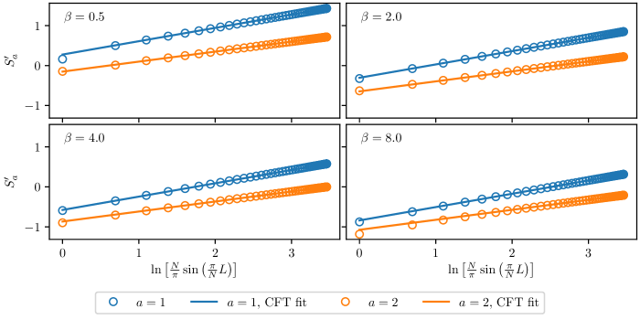
Figure 2: (Color online) Entanglement entropies in $\psi_{\beta}(\bm{s})$ in 1D with periodic boundary conditions and $N=100$ sites. The long-range behavior is consistent with the CFT expectation of Eq. (13). The quantities $S_{a}^{\prime}$ can become negative since they differ from the Rényi entropies $S_{a}$ by a divergent term, cf. Eq. (10). For the fit to the CFT formula, we chose $c=1$ and used the $10$ data points with the largest value of $L$.

For a partition of the system into two connected regions of length $L$ and $N-L$, respectively, the CFT entanglement entropy is given by Holzhey et al. (1994); Calabrese and Cardy (2004, 2009)

$$S^{\mathrm{CFT}}_{a}(L) =\frac{c}{6}\left(1+\frac{1}{a}\right)\ln\left[\frac{N}{\pi}\sin\left(\frac{\pi}{N}L\right)\right]+c_{a}^{\prime},$$ (13)

where $c$ is the central charge, $a$ the order of the Rényi entropy, and $c_{a}^{\prime}$ a non-universal constant. As shown in Fig. 2, we find good agreement between the entropy of $\psi_{\beta}(\bm{s})$ and $S^{\mathrm{CFT}}_{a}(L)$ for larger values of $L$.

For a system that has a low-energy description in terms of a Luttinger liquid, one expects Calabrese et al. (2010) subleading, oscillatory corrections to the CFT behavior of Eq. (13). For the $XXZ$ model, for example, these oscillations were found Calabrese et al. (2010) in Rényi entropies $S_{a}$ for $a\neq 1$. From Fig. 2, we conclude that such oscillations around the CFT expectation are absent for the state $\psi_{\beta}(\bm{s})$. This is in agreement with our findings about the correlations, and we interpret it as a result of the transition from discrete to continuous spins, which has a smoothing effect and thus removes the oscillatory components. We analyzed the deviation of the entanglement entropy in $\psi_{\beta}(\bm{s})$ from $S^{\mathrm{CFT}}_{a}(L)$. For large distances $L$, we find a correction to the CFT proportionality constant $\frac{c}{6}(1+\frac{1}{a})$. This deviation becomes smaller for larger systems and can thus be considered to be a finite size effect.

III.3 Entanglement spectrum

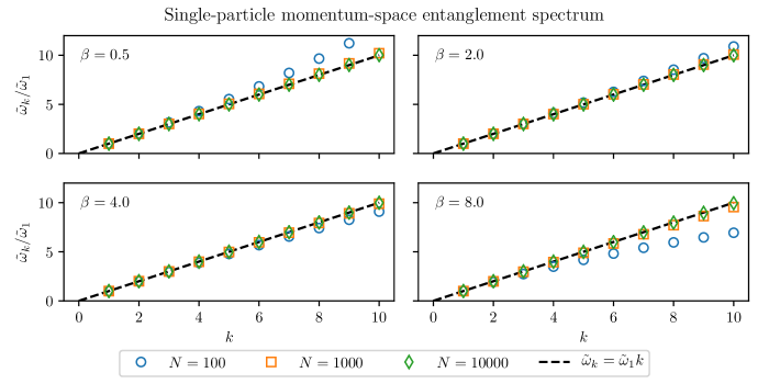
Figure 3: (Color online) Single-particle entanglement spectrum in 1D with periodic boundary conditions for a partition in momentum space. The low-lying part of the spectrum is shown for various system sizes and values of $\beta$.

To further substantiate the close connection between $\psi_{\beta}(\bm{s})$ and the free-boson CFT, we computed the entanglement spectrum for a partition in momentum space. This choice makes it possible to trace out the negative momenta, thus retaining only the chiral components Thomale et al. (2010); Lundgren et al. (2014). The details of the computation can be found in Appendix B.3. In summary, we find an entanglement Hamiltonian $\sum_{k=1}^{\lfloor\frac{N-1}{2}\rfloor}\tilde{\omega}_{k}b^{\dagger}_{k}b_{k}$, where $b_{k}$ and $b_{k}^{\dagger}$ are bosonic annihilation and creation operators, $k$ is the momentum, and $\tilde{\omega}_{k}$ are single-particle entanglement energies. We plot the low-lying part of the spectrum in Fig. 3. For large systems, we observe a linear behavior $\tilde{\omega}_{k}=k\tilde{\omega}_{1}$, where $\tilde{\omega}_{1}$ is the energy at momentum $k=1$. The entanglement spectrum is thus consistent with a chiral, massless, free boson.

III.4 Parent Hamiltonian

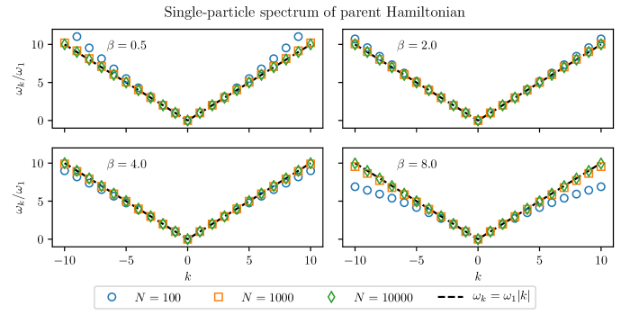
Figure 4: (Color online) Low-lying energies of the single-particle spectrum for the parent Hamiltonian of $\psi_{\beta}(\bm{s})$ in 1D with periodic boundary conditions.

We now show that $\psi_{\beta}(\bm{s})$ in 1D has a parent Hamiltonian whose low-lying energies are in agreement with the underlying CFT. The precise form of this Hamiltonian is derived in Appendix C, where we also show that it can be brought into the diagonal form $\sum_{k=1}^{N}\omega_{k}b^{\dagger}_{k}b_{k}$ in a suitable basis of annihilation and creation operators $b_{k}$ and $b_{k}^{\dagger}$. Due to translational invariance, $k$ in the single-particle energies $\omega_{k}$ has the meaning of a momentum variable in 1D.

The low-lying part of the single-particle spectrum is shown in Fig. 4. The observed linear behavior $\omega_{k}=\omega_{1}|k|$ is consistent with CFT and our findings about the momentum-space entanglement spectra. In the latter case, however, the spectrum has only chiral components since the negative momenta were traced out.

IV Properties of states in 2D

In this section, we consider a cylinder of size $N_{x}\times N_{y}$ as defined in Sec. II.5. Through a determination of the topological entanglement entropy and entanglement spectra, we provide evidence that $\psi_{\beta}(\bm{s})$ exhibits edge modes.

IV.1 Correlations

Since the spin-spin correlations do not depend on the phase of the wave function, the correlators in $\psi_{\beta}(\bm{s})$ agree with those of the approximation made in Ref. Herwerth et al., 2017, cf. Appendix D. In agreement with Ref. Herwerth et al., 2017, we find an exponential decay of spin-spin correlations in the bulk of a 2D system. The long-range edge correlations decay with a power of $-2$ independent of $\beta$, which agrees with the decay of a current-current correlator of the underlying CFT.

IV.2 Absence of intrinsic topological order

The topological order of a state can be characterized by the topological entanglement entropy Kitaev and Preskill (2006); Levin and Wen (2006) $\gamma_{\mathrm{top}}$, which occurs in the dependence of the entanglement entropy $S_{a}(A)$ on the region $A$:

$$S_{a}(A) =-\gamma_{\mathrm{top}}+b\;\partial A+\dots,$$ (14)

where $\partial A$ is the perimeter of $A$, $b$ is a non-universal constant, and the dots stand for terms that vanish for $\partial A\to\infty$. A nonzero value of $\gamma_{\mathrm{top}}$ indicates that a state exhibits intrinsic topological order.

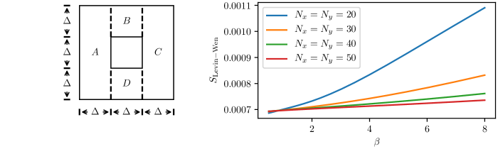
Figure 5: (Color online) Left panel: Definition of regions for the computation of the topological entanglement entropy according to Ref. Levin and Wen, 2006. The regions $A$ and $C$ are of size $\Delta\times 3\Delta$ and the regions $B$ and $D$ of size $\Delta\times\Delta$. We place the region $ABCD$ into the center of a cylinder of size $N_{x}\times N_{y}$. Right panel: Linear combination $S_{\mathrm{Levin-Wen}}$ of Eq. (15) for different system sizes and values of $\beta$. The size of $\Delta$ was chosen as $\Delta=N_{x}/5$.

The topological entanglement entropy can be computed as a linear combination of entropies for geometries that are chosen so that the terms dependent on $\partial A$ in Eq. (14) drop out Levin and Wen (2006); Kitaev and Preskill (2006). Here, we consider the construction of Levin and Wen Levin and Wen (2006) with regions as defined in the left panel of Fig. 5. For geometries that are large compared to the correlation length, $\gamma_{\mathrm{top}}$ is equal to

$$S_{\mathrm{Levin-Wen}} =\frac{1}{2}\big{[}\left(S_{1}(ABC)-S_{1}(AC)\right)$$ (15)

$$\phantom{\frac{1}{2}\big{[}}-\left(S_{1}(ABCD)-S_{1}(ADC)\right)\big{]},$$

where the Rényi index $a=1$ was chosen.

We plot $S_{\mathrm{Levin-Wen}}$ for $\psi_{\beta}(\bm{s})$ in the right panel of Fig. 5. For all considered system sizes and values of $\beta$, we observe that $S_{\mathrm{Levin-Wen}}$ is below $0.002$. Furthermore, $S_{\mathrm{Levin-Wen}}$ tends to decrease for larger systems. This indicates that the state has a vanishing topological entanglement entropy, $\gamma_{\mathrm{top}}=0$, and thus no intrinsic topological order. A similar observation of a vanishing topological entanglement entropy was made for BCS states with a $p_{x}+ip_{y}$ symmetry in Refs. Montes et al., 2017; Bray-Ali et al., 2009.

IV.3 Entanglement spectrum and edge states

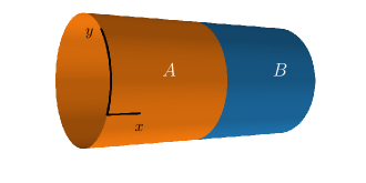
Figure 6: (Color online) Cut of the cylinder into two pieces $A$ and $B$ for the computation of the entanglement spectrum.

In the previous subsection, we provided evidence that $\psi_{\beta}(\bm{s})$ does not have intrinsic topological order. We now study the entanglement spectrum and show that it contains indications of edge states.

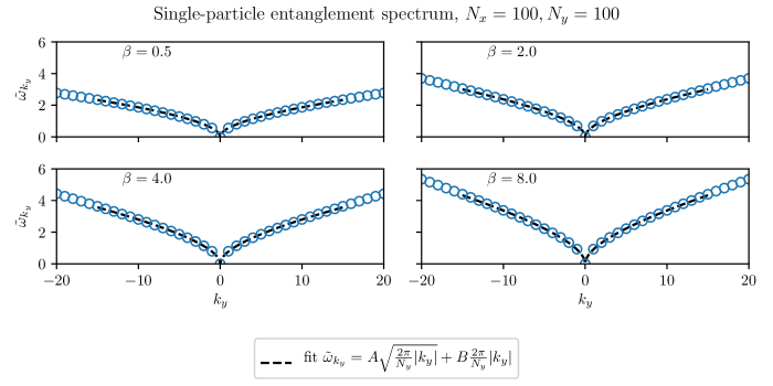
Figure 7: (Color online) Low-lying part of the single-particle entanglement spectrum in 2D for a cut of the cylinder into two pieces as shown in Fig. 6.

We consider a partition of the cylinder into two pieces of equal size, where we choose the cut perpendicular to the open direction as illustrated in Fig. 6. The low-lying part of the single-particle entanglement spectrum is shown in Fig. 7. Since the cut preserves translational symmetry, the spectrum can be ordered according to the momentum $k_{y}$ in the periodic direction. The dependence of the low-lying single-particle energies $\tilde{\omega}_{k_{y}}$ is consistent with

$$\tilde{\omega}_{k_{y}} =A\sqrt{\frac{2\pi}{N_{y}}|k_{y}|}+B\frac{2\pi}{N_{y}}|k_{y}|,$$ (16)

where $A$ and $B$ are fit constants. For large systems, we find that $A$ and $B$ are independent of the system size within variations that are due to the chosen fit range. Thus, $\omega_{k_{y}}\propto\sqrt{|k_{y}|}$ for the smallest momenta. A similar dispersion relation was recently found in the entanglement spectra of coupled Luttinger liquids Lundgren et al. (2013).

Next, we investigate whether the low-lying excited states in the entanglement spectrum are localized at the boundary created by the cut and thus represent edge excitations. To this end, we compute the basis change that makes the entanglement Hamiltonian diagonal. To exploit translational symmetry, we use Fourier transformed annihilation and creation operators $\tilde{a}_{i_{x}k_{y}}$ and $\tilde{a}_{i_{x}k_{y}}^{\dagger}$. As shown in Appendix B.4, the entanglement Hamiltonian is diagonal in annihilation and creation operators $b_{i_{x}l_{y}\sigma}$ and $b_{i_{x}l_{y}\sigma}^{\dagger}$, where $l_{y}$ is an index of non-negative momenta and $\sigma$ a sign index ($\sigma\in\{+,-\}$ for $l_{y}\notin\{0,\frac{N_{y}}{2}\}$ and $\sigma=+$ for $l_{y}\in\{0,\frac{N_{y}}{2}\}$). For $l_{y}\notin\{0,\frac{N_{y}}{2}\}$, the transformation to the diagonal basis assumes the form

$$\left(\begin{matrix}\bm{b}_{l_{y},\sigma=+}\\ \bm{b}^{\dagger}_{l_{y},\sigma=+}\end{matrix}\right) =R_{l_{y}}\frac{1}{\sqrt{2}}\left(\begin{matrix}\tilde{\bm{a}}_{l_{y}}+\tilde{\bm{a}}_{-l_{y}}\\ \tilde{\bm{a}}_{l_{y}}^{\dagger}+\tilde{\bm{a}}_{-l_{y}}^{\dagger}\\ \end{matrix}\right),$$ (17)

$$\left(\begin{matrix}\bm{b}_{l_{y},\sigma=-}\\ \bm{b}^{\dagger}_{l_{y},\sigma=-}\end{matrix}\right) =R_{l_{y}}\frac{1}{\sqrt{2}}\left(\begin{matrix}-i\tilde{\bm{a}}_{l_{y}}+i\tilde{\bm{a}}_{-l_{y}}\\ i\tilde{\bm{a}}_{l_{y}}^{\dagger}-i\tilde{\bm{a}}_{-l_{y}}^{\dagger}\\ \end{matrix}\right),$$ (18)

where $\bm{b}_{l_{y}\sigma}=(b_{i_{x}=1,l_{y},\sigma},\dots,b_{i_{x}=\frac{N_{x}}{2},l_{y},\sigma})^{t}$ and analogously for the other annihilation and creation operators. The $N_{x}\times N_{x}$ matrix $R_{l_{y}}$ is a symplectic basis transformation in the complex representation,

$$R_{l_{y}} =\left(\begin{matrix}R^{(1)}_{l_{y}}&R^{(2)}_{l_{y}}\\ \left(R^{(2)}_{l_{y}}\right)^{*}&\left(R^{(1)}_{l_{y}}\right)^{*}\end{matrix}\right).$$ (19)

We order the spectrum so that $(R^{(r)}_{l_{y}})_{i_{x}j_{x}}$ with $i_{x}=1$ and $r\in\{1,2\}$ corresponds to the lowest energy state in the sector of momentum $l_{y}$. According to Eq. (17), $\bm{b}_{l_{y}\sigma}$ are linear combinations of modes with momenta $l_{y}$ and $-l_{y}$. The two choices $\sigma\in\{+,-\}$ have the same energy and correspond to the degeneracies in Fig. 7.

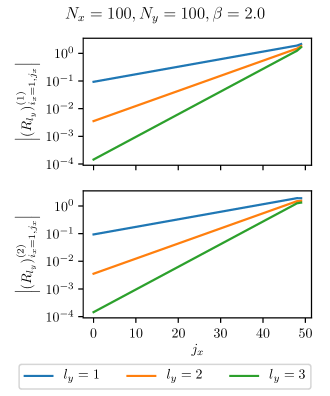
Figure 8: (Color online) Amplitude of the basis transformation for the first excited states in the entanglement spectrum of Fig. 7. The shown data is for $\beta=2.0$. (The corresponding amplitudes for $\beta\in\{0.5,4,8\}$ have the same qualitative behavior.) The lowest energy in the sector of momentum $l_{y}$ corresponds to $i_{x}=1$, cf. the explanation below Eq. (17). The value $j_{x}=50$ is the position of the cut.

Fig. 8 shows $(R^{(r)}_{l_{y}})_{i_{x}j_{x}}$ for $i_{x}=1$ and $l_{y}\in\{1,2,3\}$. We observe that $(R^{(r)}_{l_{y}})_{i_{x}j_{x}}$ falls off exponentially in $j_{x}$ for large distances to the position of the cut ($j_{x}=50$). Thus, the corresponding states are exponentially localized at the edge created by the cut. This observation provides evidence that $\psi_{\beta}(\bm{s})$ indeed supports gapless edge states.

We also did analogous computations for the local parent Hamiltonian of Appendix C to test whether its low-lying excited states are localized at the physical edges. Compared to the entanglement spectrum, we observed the following differences. First, the low-lying single-particle spectrum of the parent Hamiltonian does not consist of a single branch as the entanglement spectrum of Fig. 7. Second, we find eigenstates of the Hamiltonian with low energies that are not localized at the edge. This raises the question whether there is another parent Hamiltonian with the same low-energy behavior as observed in the entanglement spectrum.

V Conclusion

This paper considers continuous-spin wave functions $\psi_{\beta}(\bm{s})$ on lattices that are constructed as correlators of the massless, free boson CFT. In contrast to the case of discrete spins or continuous positional degrees of freedom, the wave functions $\psi_{\beta}(\bm{s})$ are Gaussian and their properties can be computed efficiently using the formalism of bosonic Gaussian states.

Through an analysis of entanglement entropies and spectra, we found that $\psi_{\beta}(\bm{s})$ is closely related to the underlying CFT in 1D. More precisely, we observed a good agreement between the entanglement entropy of $\psi_{\beta}(\bm{s})$ and the CFT expectation. In contrast to some lattice systems like the $XXZ$ model Calabrese et al. (2010), we do not find subleading oscillatory corrections to the CFT behavior. At small energies, we recovered the underlying CFT of a free, massless boson, in the momentum space entanglement spectrum and also in the spectrum of a parent Hamiltonian.

In 2D, we probed possible topological properties of $\psi_{\beta}(\bm{s})$ through an analysis of entanglement entropies and spectra. Although our results are consistent with a vanishing topological entanglement entropy, we found evidence for edge states in the entanglement spectrum. The absence of intrinsic topological order is distinct from the chiral case with discrete spins.

The wave function $\psi_{\beta}(\bm{s})$ is real since it is constructed from the full bosonic field $\varphi(z,\bar{z})$. As a consequence, the entanglement Hamiltonian in 2D has eigenstates that are linear combinations of left- and right-moving modes. Together with our observation of states localized at the edge in the low-lying entanglement spectrum, this is an indication that $\psi_{\beta}(\bm{s})$ could describe a state that is similar to a quantum spin Hall effect.

We found a local parent Hamiltonian whose low-lying energy levels in 1D are consistent with the corresponding entanglement spectrum. In 2D, however, this parent Hamiltonian has low-lying excited states that are not localized at the edge, which is in contrast to the entanglement spectrum. It would be interesting to investigate if there is another local parent Hamiltonian with the same low-energy properties as observed in the entanglement spectrum.

In 1D, the real wave function $\psi_{\beta}(\bm{s})$ is equivalent to the analogously defined chiral wave function, which is constructed from the chiral part of the free-boson field. For general lattice configurations, however, $\psi_{\beta}(\bm{s})$ differs from its chiral counterpart. In contrast to the real case, we found that the chiral state depends on the ordering of the lattice positions. It could, therefore, be that another framework than that of bosonic Gaussian states is necessary to consistently treat the chiral state, and it would be interesting to investigate this question in a future study.

Appendix A The formalism of Gaussian states

In this section, we review the formalism of bosonic Gaussian states as needed throughout this paper. In particular, we describe how to compute bipartite entanglement properties of a generic, pure Gaussian state.

We consider Gaussian wave functions

$$\psi(\bm{s}) =e^{-\frac{1}{2}\bm{s}^{t}(X+iY)\bm{s}},$$ (20)

where $\bm{s}=(s_{1},\dots,s_{N})^{t}\in\mathbb{R}^{N}$ and $X$ and $Y$ are real $N\times N$ matrices. Normalizability of the wave function $\psi(\bm{s})$ requires that $X>0$. We think of $\bm{s}$ as the vector of $N$ continuous, effective spin variables.

The wave function $\psi(\bm{s})$ has the same form as that of $N$ continuous, positional degrees on freedom on the real line. Therefore, we introduce the operators $\bm{Q}=(Q_{1},\dots,Q_{N})^{t}$ and $\bm{P}=(P_{1},\dots,P_{N})^{t}$ through

$$(Q_{m}\psi)(\bm{s}) =s_{m}\psi(\bm{s}), \text{and }(P_{m}\psi)(\bm{s}) =-i\frac{\partial\psi}{\partial s_{m}}(\bm{s}).$$ (21)

The canonical commutation relations $\left[Q_{m},P_{n}\right]=i\delta_{mn}$ can be written as

$$\left[R_{m},R_{n}\right] =i\Omega_{mn},$$ (22)

where $\bm{R}=(Q_{1},\dots,Q_{N},P_{1},\dots,P_{N})^{t}$, and $\Omega$ is the $2N\times 2N$ matrix

$$\Omega =\left(\begin{matrix}0&\mathbb{I}\\ -\mathbb{I}&0\end{matrix}\right)$$ (23)

with $\mathbb{I}$ being the $N\times N$ identity matrix. The bosonic creation and annihilation operators are defined as

$$\left(\begin{matrix}\bm{a}\\ \bm{a}^{\dagger}\end{matrix}\right) =\mathcal{U}\left(\begin{matrix}\bm{Q}\\ \bm{P}\end{matrix}\right),$$ (24)

where

$$\mathcal{U} =\frac{1}{\sqrt{2}}\left(\begin{matrix}\mathbb{I}&i\mathbb{I}\\ \mathbb{I}&-i\mathbb{I}\end{matrix}\right),$$ (25)

$\bm{a}=\left(a_{1},\dots,a_{N}\right)^{t}$, and $\bm{a}^{\dagger}=\left(a_{1}^{\dagger},\dots,a_{N}^{\dagger}\right)^{t}$. These operators satisfy the canonical commutation relations

$$\left[\left(\begin{matrix}\bm{a}\\ \bm{a}^{\dagger}\end{matrix}\right)_{m},\left(\begin{matrix}\bm{a}\\ \bm{a}^{\dagger}\end{matrix}\right)_{n}\right] =\Omega_{mn}.$$ (26)

Symplectic matrices $S$ are defined as $2N\times 2N$ real matrices satisfying $S\Omega S^{t}=\Omega$. They preserve the commutation relations of Eq. (22): Given a symplectic matrix $S$, the vector $\bm{R}^{\prime}=S\bm{R}$ satisfies $\left[R^{\prime}_{m},R_{n}^{\prime}\right]=\left[R_{m},R_{n}\right]=i\Omega_{mn}$.

A Gaussian state $\psi(\bm{s})$ is completely characterized by its covariance matrix

$$\gamma_{mn} =\frac{\langle\psi|\left\{R_{m},R_{n}\right\}|\psi\rangle}{\langle\psi|\psi\rangle},$$ (27)

where $\left\{\bullet,\bullet\right\}$ is the anticommutator.

Using the wave function of Eq. (20), one finds the covariance matrix Wolf et al. (2004); de Gosson (2006)

$$\gamma =\left(\begin{matrix}X^{-1}&-X^{-1}Y\\ -YX^{-1}&X+YX^{-1}Y\end{matrix}\right).$$ (28)

In this paper, we study entanglement properties under a partition of the system into two parts. Given a bipartition $A=\{i_{1},\dots,i_{L}\}$, $B=\{j_{1},\dots,j_{N-L}\}$ with $A\cup B=\{1,\dots,N\}$, these are encoded in the reduced density matrix $\rho_{A}$ obtained from the pure-state density matrix

$$\frac{|\psi\rangle\langle\psi|}{\langle\psi|\psi\rangle}$$ (29)

by tracing out the degrees of freedom of subsystem $B$:

$$\rho_{A} =\mathrm{tr}_{B}\frac{|\psi\rangle\langle\psi|}{\langle\psi|\psi\rangle}.$$ (30)

In terms of the covariance matrix, this operation assumes a particularly simple form. Namely, the covariance matrix $\gamma_{A}$ in the state $\rho_{A}$ obtained by tracing out the degrees of freedom in $B$ is given by removing the rows and columns corresponding to $B$ from $\gamma$. Navarrete-Benlloch (2015)

The Rényi entanglement entropy of order $a$ is defined as

$$S_{a}(A) =\frac{1}{1-a}\ln\mathrm{tr}\left[\left(\rho_{A}\right)^{a}\right],$$ (31)

where the limit $a\to 1$ corresponds to the von Neumann entropy. In terms of the covariance matrix $\gamma_{A}$ of the reduced state, the entropies $S_{a}$ can be computed as Adesso et al. (2004)

$$S_{a}(A) =\sum_{j=1}^{L}g_{a}(\nu_{j}),$$ (32)

where

$$g_{a}(y) =\frac{1}{a-1}\ln\left[\left(\frac{y+1}{2}\right)^{a}-\left(\frac{y-1}{2}\right)^{a}\right].$$ (33)

Here, $\nu_{k}$ are the symplectic eigenvalues of the matrix $\gamma_{A}$, which are the positive eigenvalues of $i\gamma_{A}\Omega$. The von Neumann entropy is given by the limit $a\to 1$:

$$\lim_{a\to 1}g_{a}(y)=\frac{y+1}{2}\ln\left(\frac{y+1}{2}\right)-\frac{y-1}{2}\ln\left(\frac{y-1}{2}\right).$$ (34)

The entanglement Hamiltonian $H_{A}$ is defined as the Hamiltonian whose thermal state is given by the reduced density matrix, $\rho_{A}=e^{-H_{A}}$. The factorization of a covariance matrix in terms of a symplectic basis transformation and a diagonal matrix consisting of symplectic eigenvalues corresponds to a decomposition into a product state of thermal oscillators Peschel and Eisler (2009); Weedbrook et al. (2012). Thus, the symplectic spectrum of the reduced state’s covariance matrix is directly related to single-particle energies of an entanglement Hamiltonian. Each symplectic eigenvalue $\nu_{j}$ corresponds to an energy

$$\tilde{\omega}_{j} =\ln\frac{\nu_{j}+1}{\nu_{j}-1}.$$ (35)

Appendix B Details on entanglement properties

This section explains how we compute entanglement properties for the Gaussian wave function $\psi_{\beta}(\bm{s})$ defined in Sec. II of the main text. With respect to the case of generic Gaussian states discussed in Appendix A, we now have to take into account the delta function in $\psi_{\beta}(\bm{s})$, which leads to divergences. The regularization explained in Sec. II.2 leads to the wave function $\psi_{\beta,\epsilon}(\bm{s})$ with covariance matrix [cf. Eq. (28)]

$$\gamma_{\beta,\epsilon} =\frac{1}{2\epsilon}\left(\begin{matrix}0&0\\ 0&\bm{e}\bm{e}^{t}\end{matrix}\right)+\gamma^{\prime}_{\beta,\epsilon},$$ (36)

where

$$\gamma^{\prime}_{\beta,\epsilon} =\left(\begin{matrix}X_{\beta,\epsilon}^{-1}&0\\ 0&X_{\beta}\end{matrix}\right).$$ (37)

Using Bartlett (1951)

$$X^{-1}_{\beta,\epsilon} =X^{-1}_{\beta}-\frac{1}{2\epsilon+\bm{e}^{t}X^{-1}_{\beta}\bm{e}}X^{-1}_{\beta}\bm{e}\bm{e}^{t}X^{-1}_{\beta},$$ (38)

we find that $\gamma_{\beta,\epsilon}^{\prime}$ is finite in the limit $\epsilon\to 0$. In particular, the $QQ$, $QP$, and $PQ$ blocks of the covariance matrix $\gamma_{\beta,\epsilon}$ are finite, while the $PP$ block has a divergent term.

B.1 Symplectic eigenvalues of the reduced state’s covariance matrix

Let us write the covariance matrix of Eq. (36) as

$$\gamma_{\beta,\epsilon} =\frac{1}{2\epsilon}vv^{t}+\gamma^{\prime}_{\beta,\epsilon}, \text{where }v =\left(\begin{matrix}0\\ \bm{e}\end{matrix}\right).$$ (39)

In the following, we consider a bipartition into disjoint subsystems $A=\{i_{1},\dots,i_{L}\}$ and $B=\{j_{1},\dots,j_{N-L}\}$, where $A\cup B=\{1,\dots,N\}$ and $L\in\{1,\dots,N-1\}$. The covariance matrix after tracing out the subsystem $B$ is given by $\mathcal{D}_{A}\gamma_{\beta,\epsilon}\mathcal{D}_{A}^{t}$, where

$$\mathcal{D}_{A} =\left(\begin{matrix}D_{A}&0\\ 0&D_{A}\end{matrix}\right)$$ (40)

with the $$L\times N$$ matrix

$$D_{A} =\left(\begin{matrix}\text{---}\bm{e}_{i_{1}}^{t}\text{---}\\ \vdots\\ \text{---}\bm{e}_{i_{L}}^{t}\text{---}\end{matrix}\right)$$ (41)

and $\bm{e}_{i}$ being the $i$th unit vector. The matrix $\mathcal{D}_{A}$ removes the rows and columns corresponding to $B$ from $\gamma_{\beta,\epsilon}$.

The entanglement entropies and spectra follow directly from the symplectic eigenvalues of $\mathcal{D}_{A}\gamma_{\beta,\epsilon}\mathcal{D}_{A}^{t}$, which are the positive eigenvalues of $i\Omega\mathcal{D}_{A}\gamma_{\beta,\epsilon}\mathcal{D}_{A}^{t}$. However, the covariance matrix $\gamma_{\beta,\epsilon}$ is divergent in the limit $\epsilon\to 0$, which leads to an infinity in the symplectic eigenvalues and thus in the entropies. To handle this divergence, we compute the inverse $\left[\mathcal{D}_{A}\gamma_{\beta,\epsilon}\mathcal{D}_{A}^{t}\right]^{-1}$ since it is finite for $\epsilon\to 0$:

$$\left[\mathcal{D}_{A}\gamma_{\beta,\epsilon}\mathcal{D}_{A}^{t}\right]^{-1} =\left[\mathcal{D}_{A}\gamma_{\beta,\epsilon}^{\prime}\mathcal{D}^{t}_{A}\right]^{-1}-\frac{\left[\mathcal{D}_{A}\gamma_{\beta,\epsilon}^{\prime}\mathcal{D}_{A}^{t}\right]^{-1}\mathcal{D}_{A}vv^{t}\mathcal{D}_{A}^{t}\left[\mathcal{D}_{A}\gamma_{\beta,\epsilon}^{\prime}\mathcal{D}_{A}^{t}\right]^{-1}}{2\epsilon+v^{t}\mathcal{D}_{A}^{t}\left[\mathcal{D}_{A}\gamma_{\beta,\epsilon}^{\prime}\mathcal{D}^{t}\right]^{-1}\mathcal{D}_{A}v},$$ (42)

where we used the formula of Ref. Bartlett, 1951 to compute the inverse of a matrix that is changed by a term of rank one. With $\mu^{(1)}_{\beta,\epsilon}\leq\mu^{(2)}_{\beta,\epsilon}\dots\leq\mu^{(L)}_{\beta,\epsilon}$ being the ordered positive eigenvalues of $-i\left[\mathcal{D}_{A}\gamma_{\beta,\epsilon}\mathcal{D}_{A}^{t}\right]^{-1}\Omega$, the symplectic spectrum of $\mathcal{D}_{A}\gamma_{\beta,\epsilon}\mathcal{D}_{A}^{t}$ is then given by $\{\nu^{(j)}_{\beta,\epsilon}=1/\mu^{(j)}_{\beta,\epsilon}\}_{1\leq j\leq{L}}$. For $\epsilon\to 0$, we have $\mu^{(1)}_{\beta,\epsilon}\to 0$ so that $\nu^{(1)}_{\beta,\epsilon}\to\infty$.

Let us now compute how $\nu^{(1)}_{\beta,\epsilon}$ scales with $\epsilon$ for $\epsilon\to 0$. This will be needed to subtract the divergence from the resulting entanglement entropy. With $\det\Omega=1$, we have

$$\ln\det\mathcal{D}_{A}\gamma_{\beta,\epsilon}\mathcal{D}_{A}^{t} =\ln\det\Omega\mathcal{D}_{A}\gamma_{\beta,\epsilon}\mathcal{D}_{A}^{t}=\sum_{j=1}^{L}\ln\left[\left(\nu^{(j)}_{\beta,\epsilon}\right)^{2}\right]$$ (43)

and therefore

$$\ln\nu^{(1)}_{\beta,\epsilon} =\frac{1}{2}\ln\det\mathcal{D}_{A}\gamma_{\beta,\epsilon}\mathcal{D}_{A}^{t}-\sum_{j=2}^{L}\ln\left[\nu^{(j)}_{\beta,\epsilon}\right].$$ (44)

The matrix determinant lemma allows to express the determinant of $\mathcal{D}_{A}\gamma_{\beta,\epsilon}\mathcal{D}_{A}^{t}$ in terms of $\mathcal{D}_{A}\gamma_{\beta,\epsilon}^{\prime}\mathcal{D}_{A}^{t}$, which differs from $\mathcal{D}_{A}\gamma_{\beta,\epsilon}\mathcal{D}_{A}^{t}$ only by a term of rank one. Thus, we obtain

$$\ln\nu^{(1)}_{\beta,\epsilon} =\frac{1}{2}\ln\left[\left(1+\frac{1}{2\epsilon}v^{t}\mathcal{D}_{A}^{t}\left(\mathcal{D}_{A}\gamma_{\beta,\epsilon}^{\prime}\mathcal{D}_{A}^{t}\right)^{-1}\mathcal{D}_{A}v\right)\det\left(\mathcal{D}_{A}\gamma_{\beta,\epsilon}^{\prime}\mathcal{D}_{A}^{t}\right)\right]-\sum_{j=2}^{L}\ln\nu^{(j)}_{\beta,\epsilon}$$ (45)

$$=-\frac{1}{2}\ln\epsilon+\ln\tilde{\nu}_{\beta}+\mathcal{O}(\epsilon),$$ (46)

where

$$\ln\tilde{\nu}_{\beta} =\frac{1}{2}\ln\left[\frac{\det\left(\mathcal{D}_{A}\gamma_{\beta,\epsilon=0}^{\prime}\mathcal{D}_{A}^{t}\right)}{2}v^{t}\mathcal{D}_{A}^{t}\left(\mathcal{D}_{A}\gamma_{\beta,\epsilon=0}^{\prime}\mathcal{D}_{A}^{t}\right)^{-1}\mathcal{D}_{A}v\right]-\sum_{j=2}^{L}\ln\nu^{(j)}_{\beta,\epsilon=0}.$$ (47)

B.2 Entanglement entropies and spectra

Having computed the symplectic spectrum $\{\nu^{(1)}_{\beta,\epsilon},\dots,\nu^{(L)}_{\beta,\epsilon}\}$ of the reduced state’s covariance matrix, we can now determine the entanglement properties in $\psi_{\beta}(\bm{s})$.

The divergent symplectic eigenvalue assumes the form $\ln\nu_{\beta,\epsilon}^{(1)}=-\frac{1}{2}\ln\epsilon+\ln\tilde{\nu}_{\beta}+\mathcal{O}(\epsilon)$ [cf. Eq. (46)], and thus we find

$$g_{a}(\nu^{(1)}_{\beta,\epsilon}) =-\frac{1}{2}\ln(\epsilon)+\frac{1}{a-1}\ln(a)-\ln(2)+\ln\tilde{\nu}_{\beta}$$ (48)

$$\quad+\mathcal{O}(\epsilon),$$

where $g_{a}(y)$ was defined in Eq. (33). From Eq. (32), the entanglement entropies then follow as

$$S_{a}(A) =-\frac{1}{2}\ln\epsilon+S_{a}^{\prime}(A)+\mathcal{O}(\epsilon),$$ (49)

where

$$S_{a}^{\prime}(A) =\frac{1}{a-1}\ln(a)-\ln(2)+\ln\tilde{\nu}_{\beta}+\sum_{j=2}^{L}g_{a}\left(\nu^{(j)}_{\beta,\epsilon=0}\right).$$ (50)

The entropy $S_{a}^{\prime}(A)$ differs from $S_{a}(A)$ by the subtraction of the divergent term $-\frac{1}{2}\ln\epsilon$.

Given the symplectic eigenvalues $\nu^{(j)}_{\beta,\epsilon}$, one can also compute the entanglement spectrum. According to Eq. (35), we find the single-particle entanglement energies

$$\tilde{\omega}_{j} =\begin{cases}0&\text{if }j=1,\\ \ln\frac{\nu^{(j)}_{\beta,\epsilon=0}+1}{\nu^{(j)}_{\beta,\epsilon=0}-1}&\text{if }j\neq 1\end{cases}$$ (51)

in the limit $\epsilon\to 0$. Since $\nu^{(1)}_{\beta,\epsilon}\to\infty$ for $\epsilon\to 0$, the energy $\tilde{\omega}_{1}$ vanishes. The entanglement Hamiltonian thus assumes the form $\sum_{j=1}^{L}\tilde{\omega}_{j}b^{\dagger}_{j}b_{j}$, where $b_{j}$ and $b^{\dagger}_{j}$ are annihilation and creation operators in a suitable basis. The precise relation between the original operators $(a_{j},a_{j}^{\dagger})$ and $(b_{j},b_{j}^{\dagger})$ can be determined by computing Williamson’s normal form Williamson (1936); de Gosson (2006) of the covariance matrix corresponding to the state’s reduced density matrix.

B.3 Momentum-space entanglement spectrum in 1D with periodic boundary conditions

We now consider the state $\psi_{\beta}(\bm{s})$ in 1D with periodic boundary conditions. For this choice, the matrix $\left(X_{\beta,\epsilon}\right)_{i,j}$ only depends on the difference $i-j$ modulo $N$, and thus we write $\left(X_{\beta,\epsilon}\right)_{i,j}=\left(X_{\beta,\epsilon}\right)_{i-j}$.

We consider the discrete Fourier transform

$$F_{kj} =\frac{1}{\sqrt{N}}e^{-2\pi i\frac{kj}{N}},$$ (52)

where the normalization was chosen so that $F$ is unitary.

Writing $F=F_{x}+iF_{y}$ with $F_{x}$ and $F_{y}$ real, we define the symplectic transformation

$$\mathcal{F} =\left(\begin{matrix}F_{x}&-F_{y}\\ F_{y}&F_{x}\end{matrix}\right),$$ (53)

which corresponds to a unitary rotation of creation and annihilation operators of the form

$$\left(\begin{matrix}\bm{a}\\ \bm{a}^{\dagger}\end{matrix}\right) \to\left(\begin{matrix}F&0\\ 0&F^{*}\end{matrix}\right)\left(\begin{matrix}\bm{a}\\ \bm{a}^{\dagger}\end{matrix}\right).$$ (54)

Therefore, $\mathcal{F}$ is the symplectic matrix that transforms to momentum space.

The covariance matrix of Eq. (36) transformed to momentum space then becomes

$$\mathcal{F}\gamma_{\beta,\epsilon}\mathcal{F}^{t} =\left(\begin{matrix}\gamma_{\beta,\epsilon}^{(1)}&0\\ 0&\gamma_{\beta,\epsilon}^{(2)}\end{matrix}\right),$$ (55)

where

$$\left(\gamma_{\beta,\epsilon}^{(1)}\right)_{k,l} =\frac{1}{2}\left[\tilde{\delta}_{k-l}\left(\left(\hat{X}_{\beta,\epsilon}\right)_{k}+\frac{1}{\left(\hat{X}_{\beta,\epsilon}\right)_{k}}\right)-\tilde{\delta}_{k+l}\left(\left(\hat{X}_{\beta,\epsilon}\right)_{k}-\frac{1}{\left(\hat{X}_{\beta,\epsilon}\right)_{k}}\right)\right],$$ (56)

$$\left(\gamma_{\beta,\epsilon}^{(2)}\right)_{k,l} =\frac{1}{2}\left[\tilde{\delta}_{k-l}\left(\left(\hat{X}_{\beta,\epsilon}\right)_{k}+\frac{1}{\left(\hat{X}_{\beta,\epsilon}\right)_{k}}\right)+\tilde{\delta}_{k+l}\left(\left(\hat{X}_{\beta,\epsilon}\right)_{k}-\frac{1}{\left(\hat{X}_{\beta,\epsilon}\right)_{k}}\right)\right],$$ (57)

$$\left(\hat{X}_{\beta,\epsilon}\right)_{k} =\sum_{j=0}^{N-1}e^{-2\pi i\frac{kj}{N}}\left(X_{\beta,\epsilon}\right)_{j},$$ (58)

and

$$\tilde{\delta}_{k} =\begin{cases}1&\text{if }k\text{ mod }N=0,\\ 0&\text{otherwise}.\end{cases}$$ (59)

Next, we trace out the momenta $k\notin A$ where $A=\{1,\dots,\lfloor\frac{N-1}{2}\rfloor\}$, i.e., we remove the negative momenta and the momenta $k\in\{0,\frac{N}{2}\}$. The resulting covariance matrix is diagonal:

$$\mathcal{D}_{A}\mathcal{F}\gamma_{\beta,\epsilon}\mathcal{F}^{t}\mathcal{D}_{A}^{t} =\bigoplus_{k=1}^{\lfloor\frac{N-1}{2}\rfloor}\frac{1}{2}\left[\left(\hat{X}_{\beta}\right)_{k}+\frac{1}{\left(\hat{X}_{\beta}\right)_{k}}\right]\oplus\bigoplus_{k=1}^{\lfloor\frac{N-1}{2}\rfloor}\frac{1}{2}\left[\left(\hat{X}_{\beta}\right)_{k}+\frac{1}{\left(\hat{X}_{\beta}\right)_{k}}\right],$$ (60)

where we replaced $\left(\hat{X}_{\beta,\epsilon}\right)_{k}$ by

$$\left(\hat{X}_{\beta}\right)_{k} =\sum_{j=0}^{N-1}e^{-2\pi i\frac{kj}{N}}\left(X_{\beta}\right)_{j}$$ (61)

since $\left(\hat{X}_{\beta}\right)_{k}=\left(\hat{X}_{\beta,\epsilon}\right)_{k}$ for $k\neq 0$. In Eq. (60), we can directly read off the symplectic eigenvalues of the reduced state’s covariance matrix as

$$\nu_{k}=\frac{1}{2}\left[\left(\hat{X}_{\beta}\right)_{k}+\frac{1}{\left(\hat{X}_{\beta}\right)_{k}}\right].$$ (62)

In a suitable basis, the entanglement Hamiltonian is thus given by $\sum_{k=1}^{\lfloor\frac{N-1}{2}\rfloor}\tilde{\omega}_{k}b^{\dagger}_{k}b_{k}$, where $b_{k}$ and $b_{k}^{\dagger}$ are bosonic annihilation and creation operators, and the entanglement energies are given by

$$\tilde{\omega}_{k} =\ln\left(\frac{\nu_{k}+1}{\nu_{k}-1}\right)=2\ln\left|\frac{\left(\hat{X}_{\beta}\right)_{k}+1}{\left(\hat{X}_{\beta}\right)_{k}-1}\right|.$$ (63)

Since we traced out the mode $k=0$, all entanglement energies are independent of $\epsilon$.

B.4 Entanglement spectrum on the cylinder

The entanglement cut of the cylinder made in Sec. IV.3 preserves translational symmetry. Therefore, it is convenient to express the eigenbasis of the entanglement Hamiltonian in terms of Fourier modes as explained in the following. The entanglement Hamiltonian is diagonal in the basis that transforms the reduced state’s covariance matrix into Williamson’s normal form.

For a cylinder of size $N_{x}\times N_{y}$ with $N_{x}$ even and coordinates defined in Eq. (11), we consider the bipartition $A=\{1,\dots,\frac{N}{2}\}$, $B=\{\frac{N}{2}+1,\dots,N\}$ corresponding to Fig. 6. The Fourier transform of the reduced state’s covariance matrix is given by

$$\mathcal{F}_{y}\gamma^{(A)}_{\beta,\epsilon}\mathcal{F}_{y}^{\dagger} =\bigoplus_{k_{y}=0}^{N_{y}-1}\gamma^{(A)}_{k_{y},\beta,\epsilon},$$ (64)

where $\gamma^{(A)}_{\beta,\epsilon}=\mathcal{D}_{A}\gamma_{\beta,\epsilon}\mathcal{D}_{A}^{t}$, and

$$\mathcal{F}_{y} =\left(\begin{matrix}F_{y}&0\\ 0&F_{y}^{*}\end{matrix}\right)$$ (65)

with

$$\left(F_{y}\right)_{i_{x}k_{y},j_{x}j_{y}} =\frac{\delta_{i_{x}j_{x}}}{\sqrt{N_{y}}}e^{-\frac{2\pi i}{N_{y}}k_{y}j_{y}}.$$ (66)

The $N_{x}\times N_{x}$ matrices $\gamma^{(A)}_{k_{y},\beta,\epsilon}$ are the blocks of the reduced state’s covariance matrix in momentum space. We note that $\gamma^{(A)}_{k_{y},\beta,\epsilon}$ is real and $\gamma^{(A)}_{k_{y},\beta,\epsilon}=\gamma^{(A)}_{-k_{y},\beta,\epsilon}$. This is a consequence of $X_{\beta,\epsilon}$ being symmetric under $i_{y}-j_{y}\to N_{y}-(i_{y}-j_{y})$ for $y$ indices $i_{y},j_{y}\in\{1,\dots,N_{y}\}$.

The matrix $\mathcal{F}_{y}$ is complex and does therefore not define a real symplectic transformation. However, we can construct a real matrix from it by combining the Fourier modes of momentum $k_{y}$ and $-k_{y}$. After this transformation, we have a description in terms of positive momenta $l_{y}\in\{0,\dots,\lfloor\frac{N_{y}}{2}\rfloor\}$ and an additional index $\sigma\in\{+,-\}$ for $l_{y}\notin\{0,\frac{N_{y}}{2}\}$ and $\sigma=+$ for $l_{y}\in\{0,\frac{N_{y}}{2}\}$. More precisely, we define the unitary matrix $T_{y}$ through its action on a vector $c_{i_{x}k_{y}}$ in Fourier space as

$$\left(T_{y}c\right)_{i_{x}l_{y}\sigma} =\begin{cases}c_{i_{x}l_{y}}&\text{if }l_{y}\in\{0,\frac{N_{y}}{2}\},\\ \frac{1}{\sqrt{2}}\left(c_{i_{x}l_{y}}+c_{i_{x},-l_{y}}\right)&\text{if }l_{y}\notin\{0,\frac{N_{y}}{2}\}\\ &\text{and }\sigma=+,\\ \frac{1}{\sqrt{2}}\left(-ic_{i_{x}l_{y}}+ic_{i_{x},-l_{y}}\right)&\text{if }l_{y}\notin\{0,\frac{N_{y}}{2}\}\\ &\text{and }\sigma=-.\end{cases}$$ (67)

Introducing

$$\mathcal{T}_{y} =\left(\begin{matrix}T_{y}&0\\ 0&T_{y}^{*}\end{matrix}\right),$$ (68)

it follows that $\mathcal{T}_{y}\mathcal{F}_{y}$ is real and symplectic. Furthermore,

$$\mathcal{T}_{y}\mathcal{F}_{y}\gamma^{(A)}_{\beta,\epsilon}\left(\mathcal{T}_{y}\mathcal{F}_{y}\right)^{t} =\bigoplus_{l_{y}=0}^{\lfloor\frac{N_{y}}{2}\rfloor}\bigoplus_{\sigma}\gamma^{(A)}_{l_{y},\beta,\epsilon},$$ (69)

which follows from $\gamma^{(A)}_{l_{y},\beta,\epsilon}=\gamma^{(A)}_{-l_{y},\beta,\epsilon}$. Using Williamson’s decomposition Williamson (1936); de Gosson (2006); Pirandola et al. (2009), we next construct symplectic matrices $R_{l_{y},\beta,\epsilon}^{\prime}$ to that

$$R_{l_{y},\beta,\epsilon}^{\prime}\gamma^{(A)}_{l_{y},\beta,\epsilon}R_{l_{y},\beta,\epsilon}^{\prime t}$$ (70)

$$\quad=\mathrm{diag}\left(\nu^{(1)}_{l_{y},\beta,\epsilon},\dots,\nu^{(\frac{N_{x}}{2})}_{l_{y},\beta,\epsilon},\nu^{(1)}_{l_{y},\beta,\epsilon},\dots,\nu^{(\frac{N_{x}}{2})}_{l_{y},\beta,\epsilon}\right).$$

The reduced state’s covariance matrix $\gamma^{(A)}_{l_{y},\beta,\epsilon}$ is thus brought into Williamson’s normal form through the transformation

$$\left(\begin{matrix}\bm{Q}^{\prime}\\ \bm{P}^{\prime}\end{matrix}\right) =R_{\beta,\epsilon}^{\prime}\mathcal{T}_{y}\mathcal{F}_{y}\left(\begin{matrix}\bm{Q}\\ \bm{P}\end{matrix}\right),$$ (71)

where

$$R_{\beta,\epsilon}^{\prime} =\bigoplus_{l_{y}=0}^{\lfloor\frac{N_{y}}{2}\rfloor}\bigoplus_{\sigma}R_{l_{y},\beta,\epsilon}^{\prime}.$$ (72)

In terms of creation and annihilation operators, this transformation is given by

$$\left(\begin{matrix}\bm{b}\\ \bm{b}^{\dagger}\end{matrix}\right) =R_{\beta,\epsilon}\mathcal{T}_{y}\mathcal{F}_{y}\left(\begin{matrix}\bm{a}\\ \bm{a}^{\dagger}\end{matrix}\right),$$ (73)

where $R_{\beta,\epsilon}=\mathcal{U}R_{\beta,\epsilon}^{\prime}\mathcal{U}^{\dagger}$, the matrix $\mathcal{U}$ is defined as in Eq. (25), and we used $\mathcal{U}\mathcal{T}_{y}\mathcal{F}_{y}\mathcal{U}^{\dagger}=\mathcal{T}_{y}\mathcal{F}_{y}$.

For the blocks with momenta $l_{y}\notin\{0,\frac{N_{y}}{2}\}$, the transformation of Eq. (73) is given by

$$\left(\begin{matrix}\bm{b}_{l_{y},\sigma=+}\\ \bm{b}^{\dagger}_{l_{y},\sigma=+}\end{matrix}\right) =R_{l_{y},\beta,\epsilon}\frac{1}{\sqrt{2}}\left(\begin{matrix}\tilde{\bm{a}}_{l_{y}}+\tilde{\bm{a}}_{-l_{y}}\\ \tilde{\bm{a}}_{l_{y}}^{\dagger}+\tilde{\bm{a}}_{-l_{y}}^{\dagger}\\ \end{matrix}\right),$$ (74)

$$\left(\begin{matrix}\bm{b}_{l_{y},\sigma=-}\\ \bm{b}^{\dagger}_{l_{y},\sigma=-}\end{matrix}\right) =R_{l_{y},\beta,\epsilon}\frac{1}{\sqrt{2}}\left(\begin{matrix}-i\tilde{\bm{a}}_{l_{y}}+i\tilde{\bm{a}}_{-l_{y}}\\ i\tilde{\bm{a}}_{l_{y}}^{\dagger}-i\tilde{\bm{a}}_{-l_{y}}^{\dagger}\\ \end{matrix}\right),$$ (75)

where $\bm{b}_{l_{y},\sigma}$ and $\tilde{\bm{a}}_{l_{y}}$ are vectors of length $\frac{N_{x}}{2}$ corresponding to $i_{x}\in\{1,\dots,\frac{N_{x}}{2}\}$, $R_{l_{y},\beta,\epsilon}$ are the blocks of $R_{\beta,\epsilon}$ defined analogously to Eq. (72), and

$$\tilde{a}_{i_{x}k_{y}} =\frac{1}{\sqrt{N_{y}}}\sum_{j_{y}=1}^{N_{y}}e^{-\frac{2\pi i}{N_{y}}j_{y}k_{y}}a_{i_{x}j_{y}}$$ (76)

are the Fourier transformed annihilation operators.

For $k_{y}\neq 0$, the blocks $\gamma^{(A)}_{\beta,\epsilon}$ and thus $R_{l_{y},\beta,\epsilon}$ do not depend on $\epsilon$, which follows from the definition of $X_{\beta,\epsilon}$ in Eq. (6). Thus, Eq. (74) leads to to Eq. (17) in the main text, where we suppressed the dependence of $R_{l_{y},\beta,\epsilon}$ on $\beta$ for better readability.

Appendix C Parent Hamiltonian

The covariance matrix in $\psi_{\beta,\epsilon}(\bm{s})$ is given by

$$\left(\begin{matrix}X^{-1}_{\beta,\epsilon}&0\\ 0&X_{\beta,\epsilon}\end{matrix}\right),$$ (77)

cf. Eq. (28). The following Hamiltonians have a ground state with the same covariance matrix and are thus parent Hamiltonians of $\psi_{\beta,\epsilon}(\bm{s})$:

$$\mathcal{H}_{\eta} =\frac{1}{2}\sum_{i,j=1}^{2N}\left(\begin{matrix}\bm{Q}\\ \bm{P}\end{matrix}\right)_{i}\left(H_{\eta}\right)_{ij}\left(\begin{matrix}\bm{Q}\\ \bm{P}\end{matrix}\right)_{j},$$ (78)

where

$$H_{\eta} =\left(\begin{matrix}X^{1+\eta}_{\beta,\epsilon}&0\\ 0&X^{-1+\eta}_{\beta,\epsilon}\end{matrix}\right),$$ (79)

$\eta$ is a real parameter, and we used a general result Schuch et al. (2006) about the relationship between a block-diagonal Hamiltonian and the corresponding ground-state covariance matrix.

To diagonalize $\mathcal{H}_{\eta}$, we choose an orthonormal eigenbasis $V_{\epsilon}$ of $X_{\beta,\epsilon}$:

$$V_{\epsilon}^{t}X_{\beta,\epsilon}V_{\epsilon} =\chi_{\beta,\epsilon},$$ (80)

where

$$\chi_{\beta,\epsilon} =\mathrm{diag}\left(c^{(1)}_{\beta,\epsilon},\dots,c^{(N)}_{\beta,\epsilon}\right).$$ (81)

[The eigenbasis $V_{\epsilon}$ is independent of $\beta$ since $X_{\beta,\epsilon}$ depends on $\beta$ through a term proportional to the identity, cf. Eq. (6).] The symplectic matrix

$$S_{\beta,\epsilon} =\left(\begin{matrix}X^{-\frac{1}{2}}_{\beta,\epsilon}V_{\epsilon}&0\\ 0&X^{\frac{1}{2}}_{\beta,\epsilon}V_{\epsilon}\end{matrix}\right)$$ (82)

transforms $H_{\eta}$ into

$$S_{\beta,\epsilon}^{t}H_{\eta}S_{\beta,\epsilon}$$ (83)

$$\quad=\mathrm{diag}\left[\left(c^{(1)}_{\beta,\epsilon}\right)^{\eta},\dots,\left(c^{(N)}_{\beta,\epsilon}\right)^{\eta},\left(c^{(1)}_{\beta,\epsilon}\right)^{\eta},\dots,\left(c^{(N)}_{\beta,\epsilon}\right)^{\eta}\right].$$

Thus, the symplectic eigenvalues of $H_{\eta}$ are given by $\left(c^{(k)}_{\beta,\epsilon}\right)^{\eta}$. Defining single-particle energies as

$$\omega_{k}=\left(c^{(k)}_{\beta,\epsilon}\right)^{\eta},$$ (84)

we thus find a parent Hamiltonian $\sum_{k=1}^{N}\omega_{k}b^{\dagger}_{k}b_{k}$ of $\psi_{\beta,\epsilon}(\bm{s})$, where the new creation and annihilation operators $\bm{b}$ and $\bm{b}^{\dagger}$ are related to the original ones ($\bm{a}$ and $\bm{a}^{\dagger}$) through

$$\left(\begin{matrix}\bm{b}\\ \bm{b}^{\dagger}\end{matrix}\right) =\frac{1}{2}\left(\begin{matrix}\chi_{\beta,\epsilon}^{\frac{1}{2}}+\chi_{\beta,\epsilon}^{-\frac{1}{2}}&\chi_{\beta,\epsilon}^{\frac{1}{2}}-\chi_{\beta,\epsilon}^{-\frac{1}{2}}\\ \chi_{\beta,\epsilon}^{\frac{1}{2}}-\chi_{\beta,\epsilon}^{-\frac{1}{2}}&\chi_{\beta,\epsilon}^{\frac{1}{2}}+\chi_{\beta,\epsilon}^{-\frac{1}{2}}\end{matrix}\right)\left(\begin{matrix}V_{\epsilon}^{t}&0\\ 0&V_{\epsilon}^{t}\end{matrix}\right)\left(\begin{matrix}\bm{a}\\ \bm{a}^{\dagger}\end{matrix}\right).$$ (85)

With $-i\frac{\partial\psi}{\partial s_{k}}(\bm{s})=i(XQ)_{k}\psi(\bm{s})$, it follows that the excited states with a single mode assume the form

$$b^{\dagger}_{k}|\psi_{\beta}\rangle =\sqrt{2}\left(\chi_{\beta,\epsilon}^{\frac{1}{2}}V_{\epsilon}^{t}\bm{Q}\right)_{k}|\psi_{\beta}\rangle.$$ (86)

The main text discusses the case $\eta=-1$, where the parent Hamiltonian becomes

$$\mathcal{H}_{\eta=-1} =\frac{1}{2}\left(\sum_{m=1}^{N}Q_{m}^{2}+\sum_{m,n=1}^{N}C_{mn}P_{m}P_{n}\right)$$ (87)

with

$$C =X_{\beta,\epsilon}^{-2}\big{|}_{\epsilon=0}=\left[X_{\beta}^{-1}-\frac{X^{-1}_{\beta}\bm{e}\bm{e}^{t}X^{-1}_{\beta}}{\bm{e}^{t}X^{-1}_{\beta}\bm{e}}\right]^{2}.$$ (88)

We did numerical computations for a uniform lattice on the circle and a square lattice on the cylinder and found that the matrix $C_{mn}$ decays with the distance between the sites $m$ and $n$. At large distances, the decay is consistent with a power law on the circle and on the edge of the cylinder and with an exponential in the bulk of the cylinder.

Appendix D Relation to lattice states obtained from conformal field theory

We now relate the wave functions $\psi_{\beta}(\bm{s})$ with $s_{j}$ continuous to a class of lattice states $\psi_{\alpha}$ with discrete spin-$\frac{1}{2}$ degrees of freedom constructed from CFT. The latter are defined as

$$|\psi_{\alpha}\rangle =\sum_{s_{1},\dots,s_{N}}\psi_{\alpha}(s_{1},\dots,s_{N})|s_{1},\dots,s_{N}\rangle,$$ (89)

$$\psi_{\alpha}(s_{1},\dots,s_{N}) =\langle:e^{i\sqrt{\alpha}s_{1}\varphi(z_{1})}:\dots:e^{i\sqrt{\alpha}s_{N}\varphi(z_{N})}:\rangle$$ (90)

$$=\delta_{\bm{s}}\prod_{m<n}(z_{m}-z_{n})^{\alpha s_{m}s_{n}}$$ (91)

where $\delta_{\bm{s}}=1$ if $s_{1}+\dots+s_{N}=0$ and $\delta_{\bm{s}}=0$ otherwise, $\alpha>0$ is a real parameter, $s_{i}\in\{-1,1\}$, and $|s_{1},\dots,s_{N}\rangle$ is the product of eigenstates $|s_{j}\rangle$ of the spin-$z$ operator at lattice site $j$ ($t^{z}_{j}|s_{j}\rangle=\frac{1}{2}s_{j}|s_{j}\rangle$).

In a previous study Herwerth et al. (2017), we considered $zz$ correlations $C_{ij}$ in $\psi_{\alpha}$,

$$C_{ij}\equiv 4\frac{\langle\psi_{\alpha}|t^{z}_{i}t^{z}_{j}|\psi_{\alpha}\rangle}{\langle\psi_{\alpha}|\psi_{\alpha}\rangle} =\frac{\sum_{s_{1},\dots,s_{N}}s_{i}s_{j}\delta_{\bm{s}}\prod_{m<n}|z_{m}-z_{n}|^{2\alpha s_{m}s_{n}}}{\sum_{s_{1},\dots,s_{N}}\delta_{\bm{s}}\prod_{m<n}|z_{m}-z_{n}|^{2\alpha s_{m}s_{n}}},$$ (92)

and approximated them for $i\neq j$ by a continuous integral of the form

$$C_{ij}^{(\mathrm{approx})}=\frac{\int d^{N}\bm{s}s_{i}s_{j}\delta\left(s_{1}+\dots+s_{N}\right)e^{-\frac{1}{2}\bm{s}^{2}}\prod_{m<n}\left|\lambda\left(z_{m}-z_{n}\right)\right|^{2\alpha s_{m}s_{n}}}{\int d^{N}\bm{s}\delta\left(s_{1}+\dots+s_{N}\right)e^{-\frac{1}{2}\bm{s}^{2}}\prod_{m<n}\left|\lambda(z_{m}-z_{n})\right|^{2\alpha s_{m}s_{n}}},$$ (93)

where $\lambda>0$ is a scale parameter that we fixed by requiring that the subleading term of the approximation is minimal.

Rescaling $s_{j}\to s_{j}/\sqrt{\alpha}$ in $C^{(\mathrm{approx})}_{ij}$ and using $\prod_{m<n}\lambda^{s_{m}s_{n}}=e^{-\frac{1}{2}\bm{s}^{2}\ln\lambda}$ for $s_{1}+\dots+s_{N}=0$, we find

$$C^{(\mathrm{approx})}_{ij} =\frac{1}{\alpha}\frac{\int d^{N}\bm{s}s_{i}s_{j}\delta\left(s_{1}+\dots+s_{N}\right)e^{-\frac{1}{2}\bm{s}^{2}\left(\frac{1}{\alpha}+2\ln\lambda\right)}\prod_{m<n}\left|z_{m}-z_{n}\right|^{2s_{m}s_{n}}}{\int d^{N}\bm{s}\delta\left(s_{1}+\dots+s_{N}\right)e^{-\frac{1}{2}\bm{s}^{2}\left(\frac{1}{\alpha}+2\ln\lambda\right)}\prod_{m<n}\left|z_{m}-z_{n}\right|^{2s_{m}s_{n}}}$$ (94)

$$=\frac{1}{\alpha}\frac{\int d^{N}\bm{s}s_{i}s_{j}|\psi_{\beta}(\bm{s})|^{2}}{\int d^{N}\bm{s}|\psi_{\beta}(\bm{s})|^{2}},$$ (95)

where we identified $\beta+\beta_{0}=\frac{1}{\alpha}+2\ln\lambda$. Thus, the approximation $C^{(\mathrm{approx})}_{ij}$ made in Ref. Herwerth et al., 2017 corresponds to the spin-spin correlations of the wave function $\psi_{\beta}(\bm{s})$ up to a total factor of $\frac{1}{\alpha}$. The same is true for the chiral state $\tilde{\psi}_{\beta}(\bm{s})$ of Sec. E since $\psi_{\beta}(\bm{s})$ and $\tilde{\psi}_{\beta}(\bm{s})$ only differ by a phase and thus have the same spin-spin correlations.

Appendix E Chiral state

The chiral analog of $\psi_{\beta}(\bm{s})$ has the form

$$\tilde{\psi}_{\beta}(\bm{s}) =e^{-\frac{1}{4}\left(\beta+\beta_{0}\right)\bm{s}^{2}}\langle:e^{is_{1}\varphi(z_{1})}:\dots:e^{is_{N}\varphi(z_{N})}:\rangle$$ (96)

$$=e^{-\frac{1}{4}\left(\beta+\beta_{0}\right)\bm{s}^{2}}\delta\left(s_{1}+\dots+s_{N}\right)$$

$$\quad\times\prod_{m<n}\left(z_{m}-z_{n}\right)^{s_{m}s_{n}},$$

where $\varphi(z)$ is the chiral part of the free boson according to the decomposition $\varphi(z,\bar{z})=\varphi(z)+\bar{\varphi}(\bar{z})$.

On the cylinder introduced in Sec. II.5, the chiral wave function assumes the form

$$\tilde{\psi}_{\beta}(\bm{s}) =e^{-\frac{1}{4}\left(\beta+\beta_{0}\right)\bm{s}^{2}}\langle:e^{is_{1}\varphi(w_{1})}:\dots:e^{is_{N}\varphi(w_{N})}:\rangle$$ (97)

$$=e^{-\frac{1}{4}\left(\beta+\beta_{0}\right)\bm{s}^{2}}\delta\left(s_{1}+\dots+s_{N}\right)$$

$$\quad\times\prod_{m<n}\left[2\sinh\left(\frac{1}{2}(w_{m}-w_{n})\right)\right]^{s_{m}s_{n}}.$$

We now show that $\psi_{\beta}(\bm{s})$ is equivalent to $\tilde{\psi}_{\beta}(\bm{s})$ for a uniform lattice in 1D with periodic boundary conditions. Setting $N_{x}=1$ in Eqs. (11) and (97), we have

$$\tilde{\psi}_{\beta}(\bm{s}) =\delta\left(s_{1}+\dots+s_{N}\right)e^{-\frac{1}{4}(\beta+\beta_{0})\bm{s}^{2}}$$ (98)

$$\quad\quad\times\prod_{m<n}^{N}\left[2i\sin\left(\frac{\pi}{N}(m-n)\right)\right]^{s_{m}s_{n}}$$

$$=e^{i\frac{\pi}{4}\bm{s}^{2}}\delta\left(s_{1}+\dots+s_{N}\right)e^{-\frac{1}{4}(\beta+\beta_{0})\bm{s}^{2}}$$

$$\quad\quad\times\prod_{m<n}^{N}\left[2\sin\left(\frac{\pi}{N}(n-m)\right)\right]^{s_{m}s_{n}}$$

$$=e^{i\frac{\pi}{4}\bm{s}^{2}}\psi_{\beta}(\bm{s}),$$

where we used that $s_{1}+\dots+s_{N}=0$. Up to the phase factor $e^{i\frac{\pi}{4}\bm{s}^{2}}$, the wave function $\tilde{\psi}_{\beta}(\bm{s})$ thus coincides with $\psi_{\beta}(\bm{s})$. Since $e^{i\frac{\pi}{4}\bm{s}^{2}}$ is a product of local phase factors, it does not influence the spin-spin correlations and entanglement entropies. Furthermore, it can be transformed away through the symplectic transformation

$$\left(\begin{matrix}\bm{Q}\\ \bm{P}\end{matrix}\right) \to\left(\begin{matrix}\mathbb{I}&0\\ -\frac{\pi}{2}\mathbb{I}&\mathbb{I}\end{matrix}\right)\left(\begin{matrix}\bm{Q}\\ \bm{P}\end{matrix}\right).$$ (99)

For generic lattice configurations, however, an important difference between the real wave function $\psi_{\beta}(\bm{s})$ and the chiral $\tilde{\psi}_{\beta}(\bm{s})$ is that the former is independent of the lattice ordering while the latter is not. More precisely, $\psi_{\beta}(\bm{s})$ is symmetric under a simultaneous permutation $\sigma$ of both the spins $s_{j}$ and the positions $z_{j}$:

$$\psi_{\beta}^{(z_{\sigma(1)},\dots,z_{\sigma(N)})}(s_{\sigma(1)},\dots,s_{\sigma(N)}) =\psi_{\beta}^{(z_{1},\dots,z_{N})}(s_{1},\dots,s_{N}),$$ (100)

where we explicitly wrote the parametric dependence of $\psi_{\beta}(\bm{s})$ on the lattice positions. This symmetry does, however, not hold in the chiral case. The permutation $\sigma(j)=N-j+1$, for example, changes the wave function according to

$$\tilde{\psi}_{\beta}^{(z_{\sigma(1)},\dots,z_{\sigma(N)})}(s_{\sigma(1)},\dots,s_{\sigma(N)})$$ (101)

$$\quad=\prod_{m<n}e^{\pi is_{m}s_{n}\Phi_{nm}}\tilde{\psi}_{\beta}^{(z_{1},\dots,z_{N})}(s_{1},\dots,s_{N}),$$

where $\Phi_{mn}=\frac{1}{\pi}\left[\mathrm{arg}(z_{m}-z_{n})-\mathrm{arg}(z_{n}-z_{m})\right]$, and we explicitly wrote the parametric dependence on $z_{j}$. The phase $\prod_{m<n}e^{\pi is_{m}s_{n}\Phi_{nm}}$ does not change the spin-spin correlations in $\tilde{\psi}_{\beta}(\bm{s})$, but it influences entanglement properties since it is in general not a product of single-particle phase factors.

References

- Laughlin (1983) R. B. Laughlin, “Anomalous Quantum Hall Effect: An Incompressible Quantum Fluid with Fractionally Charged Excitations,” Phys. Rev. Lett. 50, 1395 (1983).
- Haldane (1983) F. D. M. Haldane, “Fractional Quantization of the Hall Effect: A Hierarchy of Incompressible Quantum Fluid States,” Phys. Rev. Lett. 51, 605 (1983).
- Halperin (1984) B. I. Halperin, “Statistics of Quasiparticles and the Hierarchy of Fractional Quantized Hall States,” Phys. Rev. Lett. 52, 2390 (1984).
- Moore and Read (1991) G. Moore and N. Read, “Nonabelions in the fractional quantum Hall effect,” Nucl. Phys. B 360, 362 (1991).
- Tsui et al. (1982) D. C. Tsui, H. L. Stormer, and A. C. Gossard, “Two-Dimensional Magnetotransport in the Extreme Quantum Limit,” Phys. Rev. Lett. 48, 1559 (1982).
- Wen (1990a) X. G. Wen, “Topological Orders in Rigid States,” Int. J. Mod. Phys. B 4, 239 (1990a).
- Wen (2016) X.-G. Wen, “A theory of 2+1D bosonic topological orders,” Natl. Sci. Rev. 3, 68 (2016).
- Calogero (1969) F. Calogero, “Ground State of a One-Dimensional -Body System,” J. Math. Phys. 10, 2197 (1969).
- Calogero (1971) F. Calogero, “Solution of the One-Dimensional -Body Problems with Quadratic and/or Inversely Quadratic Pair Potentials,” J. Math. Phys. 12, 419 (1971).
- Sutherland (1971a) B. Sutherland, “Quantum Many-Body Problem in One Dimension: Ground State,” J. Math. Phys. 12, 246 (1971a).
- Sutherland (1971b) B. Sutherland, “Exact Results for a Quantum Many-Body Problem in One Dimension,” Phys. Rev. A 4, 2019 (1971b).
- Sørensen et al. (2005) A. S. Sørensen, E. Demler, and M. D. Lukin, “Fractional Quantum Hall States of Atoms in Optical Lattices,” Phys. Rev. Lett. 94, 086803 (2005).
- Hafezi et al. (2007) M. Hafezi, A. S. Sørensen, E. Demler, and M. D. Lukin, “Fractional quantum Hall effect in optical lattices,” Phys. Rev. A 76, 023613 (2007).
- Cooper and Dalibard (2013) N. R. Cooper and J. Dalibard, “Reaching Fractional Quantum Hall States with Optical Flux Lattices,” Phys. Rev. Lett. 110, 185301 (2013).
- Yao et al. (2013) N. Y. Yao, A. V. Gorshkov, C. R. Laumann, A. M. Läuchli, J. Ye, and M. D. Lukin, “Realizing Fractional Chern Insulators in Dipolar Spin Systems,” Phys. Rev. Lett. 110, 185302 (2013).
- Goldman et al. (2016) N Goldman, J. C. Budich, and P. Zoller, “Topological quantum matter with ultracold gases in optical lattices,” Nat. Phys. 12, 639 (2016).
- Bloch et al. (2008) I. Bloch, J. Dalibard, and W. Zwerger, “Many-body physics with ultracold gases,” Rev. Mod. Phys. 80, 885 (2008).
- Aidelsburger et al. (2013) M. Aidelsburger, M. Atala, M. Lohse, J. T. Barreiro, B. Paredes, and I. Bloch, “Realization of the Hofstadter Hamiltonian with Ultracold Atoms in Optical Lattices,” Phys. Rev. Lett. 111, 185301 (2013).
- Miyake et al. (2013) H. Miyake, G. A. Siviloglou, C. J. Kennedy, W. C. Burton, and W. Ketterle, “Realizing the Harper Hamiltonian with Laser-Assisted Tunneling in Optical Lattices,” Phys. Rev. Lett. 111, 185302 (2013).
- Lohse et al. (2018) M. Lohse, C. Schweizer, H. M. Price, O. Zilberberg, and I. Bloch, “Exploring 4D quantum Hall physics with a 2D topological charge pump,” Nature 553, 55 (2018).
- Zilberberg et al. (2018) O. Zilberberg, S. Huang, J. Guglielmon, M. Wang, K. P. Chen, Y. E. Kraus, and M. C. Rechtsman, “Photonic topological boundary pumping as a probe of 4D quantum Hall physics,” Nature 553, 59 (2018).
- Kalmeyer and Laughlin (1987) V. Kalmeyer and R. B. Laughlin, “Equivalence of the resonating-valence-bond and fractional quantum Hall states,” Phys. Rev. Lett. 59, 2095 (1987).
- Kalmeyer and Laughlin (1989) V. Kalmeyer and R. B. Laughlin, “Theory of the spin liquid state of the Heisenberg antiferromagnet,” Phys. Rev. B 39, 11879 (1989).
- Greiter and Thomale (2009) M. Greiter and R. Thomale, “Non-Abelian Statistics in a Quantum Antiferromagnet,” Phys. Rev. Lett. 102, 207203 (2009).
- Haldane (1988) F. D. M. Haldane, “Exact Jastrow-Gutzwiller resonating-valence-bond ground state of the spin-1/2 antiferromagnetic Heisenberg chain with exchange,” Phys. Rev. Lett. 60, 635 (1988).
- Shastry (1988) B. S. Shastry, “Exact solution of an Heisenberg antiferromagnetic chain with long-ranged interactions,” Phys. Rev. Lett. 60, 639 (1988).
- Thomale et al. (2009) R. Thomale, E. Kapit, D. F. Schroeter, and M. Greiter, “Parent Hamiltonian for the chiral spin liquid,” Phys. Rev. B 80, 104406 (2009).
- Nielsen et al. (2012) A. E. B. Nielsen, J. I. Cirac, and G. Sierra, “Laughlin Spin-Liquid States on Lattices Obtained from Conformal Field Theory,” Phys. Rev. Lett. 108, 257206 (2012).
- Nielsen et al. (2013) A. E. B. Nielsen, G. Sierra, and J. I. Cirac, “Local models of fractional quantum Hall states in lattices and physical implementation,” Nat. Commun. 4, 2864 (2013).
- Halperin (1982) B. I. Halperin, “Quantized Hall conductance, current-carrying edge states, and the existence of extended states in a two-dimensional disordered potential,” Phys. Rev. B 25, 2185 (1982).
- Wen (1990b) X. G. Wen, “Chiral Luttinger liquid and the edge excitations in the fractional quantum Hall states,” Phys. Rev. B 41, 12838 (1990b).
- Wen (1990c) X. G. Wen, “Electrodynamical properties of gapless edge excitations in the fractional quantum Hall states,” Phys. Rev. Lett. 64, 2206 (1990c).
- Wen (1991) X. G. Wen, “Gapless boundary excitations in the quantum Hall states and in the chiral spin states,” Phys. Rev. B 43, 11025 (1991).
- Wen (1992) X.-G. Wen, “Theory of the edge states in fractional quantum Hall effects,” Int. J. Mod. Phys. B 6, 1711 (1992).
- Dubail et al. (2012) J. Dubail, N. Read, and E. H. Rezayi, “Edge-state inner products and real-space entanglement spectrum of trial quantum Hall states,” Phys. Rev. B 86, 245310 (2012).
- Witten (1989) E. Witten, “Quantum field theory and the Jones polynomial,” Commun. Math. Phys. 121, 351 (1989).
- Cirac and Sierra (2010) J. I. Cirac and G. Sierra, “Infinite matrix product states, conformal field theory, and the Haldane-Shastry model,” Phys. Rev. B 81, 104431 (2010).
- Nielsen et al. (2011) A. E. B. Nielsen, J. I. Cirac, and G. Sierra, “Quantum spin Hamiltonians for the SU(2)k WZW model,” J. Stat. Mech. 2011, P11014 (2011).
- Klitzing et al. (1980) K. v. Klitzing, G. Dorda, and M. Pepper, “New Method for High-Accuracy Determination of the Fine-Structure Constant Based on Quantized Hall Resistance,” Phys. Rev. Lett. 45, 494 (1980).
- Tu et al. (2014) H.-H. Tu, A. E. B. Nielsen, J. I. Cirac, and G. Sierra, “Lattice Laughlin states of bosons and fermions at filling fractions ,” New J. Phys. 16, 033025 (2014).
- Glasser et al. (2016) I. Glasser, J. I. Cirac, G. Sierra, and A. E. B. Nielsen, “Lattice effects on Laughlin wave functions and parent Hamiltonians,” Phys. Rev. B 94, 245104 (2016).
- Herwerth et al. (2017) B. Herwerth, G. Sierra, J. I. Cirac, and A. E. B. Nielsen, “Effective description of correlations for states obtained from conformal field theory,” Phys. Rev. B 96, 115139 (2017).
- Vidal et al. (2003) G. Vidal, J. I. Latorre, E. Rico, and A. Kitaev, “Entanglement in Quantum Critical Phenomena,” Phys. Rev. Lett. 90, 227902 (2003).
- Calabrese and Cardy (2004) P. Calabrese and J. Cardy, “Entanglement entropy and quantum field theory,” J. Stat. Mech. 2004, P06002 (2004).
- Kitaev and Preskill (2006) A. Kitaev and J. Preskill, “Topological Entanglement Entropy,” Phys. Rev. Lett. 96, 110404 (2006).
- Levin and Wen (2006) M. Levin and X.-G. Wen, “Detecting Topological Order in a Ground State Wave Function,” Phys. Rev. Lett. 96, 110405 (2006).
- Li and Haldane (2008) H. Li and F. D. M. Haldane, “Entanglement Spectrum as a Generalization of Entanglement Entropy: Identification of Topological Order in Non-Abelian Fractional Quantum Hall Effect States,” Phys. Rev. Lett. 101, 010504 (2008).
- Kane and Mele (2005a) C. L. Kane and E. J. Mele, “Quantum Spin Hall Effect in Graphene,” Phys. Rev. Lett. 95, 226801 (2005a).
- Kane and Mele (2005b) C. L. Kane and E. J. Mele, “ Topological Order and the Quantum Spin Hall Effect,” Phys. Rev. Lett. 95, 146802 (2005b).
- Bernevig and Zhang (2006) B. A. Bernevig and S.-C. Zhang, “Quantum Spin Hall Effect,” Phys. Rev. Lett. 96, 106802 (2006).
- Bartlett (1951) M. S. Bartlett, “An Inverse Matrix Adjustment Arising in Discriminant Analysis,” Ann. Math. Statist. 22, 107 (1951).
- Di Francesco et al. (1997) P. Di Francesco, P. Mathieu, and D. Sénéchal, Conformal Field Theory, Graduate Texts in Contemporary Physics (Springer, New York, 1997).
- Luther and Peschel (1975) A. Luther and I. Peschel, “Calculation of critical exponents in two dimensions from quantum field theory in one dimension,” Phys. Rev. B 12, 3908 (1975).
- Holzhey et al. (1994) C. Holzhey, F. Larsen, and F. Wilczek, “Geometric and renormalized entropy in conformal field theory,” Nucl. Phys. B 424, 443 (1994).
- Calabrese and Cardy (2009) P. Calabrese and J. Cardy, “Entanglement entropy and conformal field theory,” J. Phys. A: Math. Theor. 42, 504005 (2009).
- Calabrese et al. (2010) P. Calabrese, M. Campostrini, F. Essler, and B. Nienhuis, “Parity Effects in the Scaling of Block Entanglement in Gapless Spin Chains,” Phys. Rev. Lett. 104, 095701 (2010).
- Thomale et al. (2010) R. Thomale, D. P. Arovas, and B. A. Bernevig, “Nonlocal Order in Gapless Systems: Entanglement Spectrum in Spin Chains,” Phys. Rev. Lett. 105, 116805 (2010).
- Lundgren et al. (2014) R. Lundgren, J. Blair, M. Greiter, A. Läuchli, G. A. Fiete, and R. Thomale, “Momentum-Space Entanglement Spectrum of Bosons and Fermions with Interactions,” Phys. Rev. Lett. 113, 256404 (2014).
- Montes et al. (2017) S. Montes, J. Rodríguez-Laguna, and G. Sierra, “BCS wave function, matrix product states, and the Ising conformal field theory,” Phys. Rev. B 96, 195152 (2017).
- Bray-Ali et al. (2009) N. Bray-Ali, L. Ding, and S. Haas, “Topological order in paired states of fermions in two dimensions with breaking of parity and time-reversal symmetries,” Phys. Rev. B 80, 180504 (2009).
- Lundgren et al. (2013) R. Lundgren, Y. Fuji, S. Furukawa, and M. Oshikawa, “Entanglement spectra between coupled Tomonaga-Luttinger liquids: Applications to ladder systems and topological phases,” Phys. Rev. B 88, 245137 (2013).
- Wolf et al. (2004) M. M. Wolf, G. Giedke, O. Krüger, R. F. Werner, and J. I. Cirac, “Gaussian entanglement of formation,” Phys. Rev. A 69, 052320 (2004).
- de Gosson (2006) M. de Gosson, Symplectic Geometry and Quantum Mechanics, Operator Theory: Advances and Applications (Birkhäuser, Basel, 2006).
- Navarrete-Benlloch (2015) C. Navarrete-Benlloch, An Introduction to the Formalism of Quantum Information with Continuous Variables (Morgan & Claypool Publishers, San Rafael, 2015).
- Adesso et al. (2004) G. Adesso, A. Serafini, and F. Illuminati, “Extremal entanglement and mixedness in continuous variable systems,” Phys. Rev. A 70, 022318 (2004).
- Peschel and Eisler (2009) I. Peschel and V. Eisler, “Reduced density matrices and entanglement entropy in free lattice models,” J. Phys. A: Math. Theor. 42, 504003 (2009).
- Weedbrook et al. (2012) C. Weedbrook, S. Pirandola, R. García-Patrón, N. J. Cerf, T. C. Ralph, J. H. Shapiro, and S. Lloyd, “Gaussian quantum information,” Rev. Mod. Phys. 84, 621 (2012).
- Williamson (1936) J. Williamson, “On the Algebraic Problem Concerning the Normal Forms of Linear Dynamical Systems,” Am. J. Math. 58, 141 (1936).
- Pirandola et al. (2009) S. Pirandola, A. Serafini, and S. Lloyd, “Correlation matrices of two-mode bosonic systems,” Phys. Rev. A 79, 052327 (2009).
- Schuch et al. (2006) N. Schuch, J. I. Cirac, and M. M. Wolf, “Quantum States on Harmonic Lattices,” Commun. Math. Phys. 267, 65 (2006).