Directed Continuous-Time Random Walk with memory

Abstract

We propose a new Directed Continuous-Time Random Walk (CTRW) model with memory. As CTRW trajectory consists of spatial jumps preceded by waiting times, in Directed CTRW, we consider the case with only positive spatial jumps. Moreover, we consider the memory in the model as each spatial jump depends on the previous one. Our model is motivated by the financial application of the CTRW presented in [Phys. Rev. E 82:046119][Eur. Phys. J. B 90:50]. As CTRW can successfully describe the short term negative autocorrelation of returns in high-frequency financial data (caused by the bid-ask bounce phenomena), we asked ourselves to what extent the observed long-term autocorrelation of absolute values of returns can be explained by the same phenomena. It turned out that the bid-ask bounce can be responsible only for the small fraction of the memory observed in the high-frequency financial data.

1 Introduction

In 1956 two physicists Montroll and Weiss, in the context of dispersive transport diffusion, introduced a new stochastic process they named Continuous-Time Random Walk (CTRW) montroll1965 . As dynamics of many complex systems can be described by discrete spatiotemporal events, i.e., the spatial jump of stochastic process preceded by waiting time, the formalism of CTRW seems a natural description. On the other hand, CTRW can be considered as a way to introduce finite, continuous and fluctuating interevent times into a random walk.

Since its introduction, the elegant and flexible concept of CTRW found many applications and inspired at least three generations of scientists. It is worth to mention that recently The European Physical Journal B published a special issue titled ”Continuous Time Random Walk fifty years on”. The extended introduction to this topical issue by Kutner and Masoliver lists all applications and extensions of CTRW created up to 2017 Kutner2017 .

CTRW was initially introduced to describe a photocurrent relaxation in amorphous films SM ; pfister1978 ; shlesinger1984 ; weiss1994 ; bouchaud1990 . A broad spectrum of other applications and arrangements contains: diffusion in probabilistic fractal structures (percolations clusters ben2000 and fractal diffusion HILFER200335 ), aging of glasses EB ; MB , nearly constant dielectric loss in disordered ionic conductors dieterich2009 , cardiological rhythms iyengar1996 , electron transfer nelson1999 , search models lomholt2008 , transport in porous media margolin2000 , diffusion of epicenters of earthquakes aftershocks HS , subsurface tracer diffusion scher2002 , hydrogen diffusion in nanostructure compounds hempelmann1999 or even human travel hufnagel2006 . In this work we are particularly interested in CTRW models used in the description of financial markets, mainly financial time series, where the dependencies and distributions of times between transactions and price changes are considered f1 ; f2 ; f3 ; f4 ; f5 ; f6 ; f7 ; f8 ; f9 ; f10 ; kutner2002 ; scalas2006 ; perello2008 ; Gubiec2017 ; TG_1 ; kasprzak2010 .

In the majority of cases, the analyzed CTRW models focus on the spatial distribution with zero mean or even symmetric distribution. In other words, the drift term is usually neglected. The case of drift was studied in metzler2000 (and references therein). The case of canonical CTRW, where both spatial and temporal distributions are i.i.d. and they do not depend on each other, turns out to be a compelling model, able to describe many cases of normal or anomalous diffusion. Different types of CTRW are obtained if mean waiting time is finite or diverging (but assuming finite variance of the spatial distribution). In the first case, we observe a normal diffusion, in the latter subdiffusion occurs scher1991 . If the variance of the spatial distribution diverges and waiting time distribution has a finite mean, we obtain the description of Lévy flights.

The other promising branch of CTRW models is the one considering memory, i.e., the dependence between successive jumps. Different types of dependencies were already studied: the backward or forward correlations between spatial jump directions haus1987 in the case of concentrated lattice gas for the study of the tracer coefficient kehr1981 , even taking into account the dependencies over several subsequent jumps kutner1985 . Also, models driven by the negative feedback in consecutive jumps were built, considering one-step memory TG_0 ; TG_1 and later two-step or even infinity-step memory Gubiec2017 . Their potential applications cover the Le Chatelier-Braun principle of contrariness. Memory in waiting times also appeared in some CTRW models montero2007 ; montero2011 ; metzler2010 ; zebrowski2012 ; sokolov2009 ; metzler2013 . Examples of used dependencies are correlations which solely depends on the sign of consecutive jumps montero2007 , random walk of waiting times zebrowski2012 ; metzler2010 , exponential and slowly decaying persistent power-law correlationssokolov2009 .

Our work is directly motivated by the application of CTRW in the description of high-frequency financial data. The universal properties of all financial price time series are sometimes referred to as stylized facts Tsay ; RCont2001 . There are two well known stylized facts about autocorrelation of price time series. The first one states that the time-dependent autocorrelation of price increments (or logarithmic returns) is negative and quickly decays to zero montero2007 . A CTRW model with memory TG_1 successfully reproduced this fact. The second stylized fact states that autocorrelation of the absolute value of price increments (or absolute values of log returns) is a positive slowly decaying function. Also, the amplitude in the second case is usually an order of magnitude higher than in the first case. It is the reminiscence of the so-called volatility clustering phenomenon RCont2005 . It seems natural to ask if the CTRW model with memory introduced in TG_1 adapted to describe absolute values of price changes can successfully reproduce the second mentioned stylized fact. We are answering this question below.

The paper is organized as follows: in Section 2 we present the motivation of our work and define and solve the proper stochastic process. In Section 3 we obtain Velocity Autocorrelation Function (VAF) and in Section 4 the comparison with empirical data is made. The intraday-seasonality is taken into account in Section 5. Finally in Section 6 we conclude with some additional remarks the results presented in this paper.

2 Model

We construct a directed continuous-time random walk (CTRW) process with assumptions analogical to ones used in TG_1 but focused on the absolute values of spatial jumps. This process models stock prices, the value of the process at time $t$ represents the stock price at the corresponding time. A change of its value, called jump, is the price change (which happens immediately when transaction occurs). Waiting time can be interpreted as the time between transactions. We consider one-step memory for consecutive jumps and no dependence between waiting times or between waiting times and jumps. To consider modules of jumps, we create a new process based on the original one. We insert jump length modules in the place of jumps. We obtain directed process, where one-step memory for consecutive jumps is given by

$$H(R_{n}|R_{n-1})=(1-\epsilon)H(R_{n})+\epsilon\delta(R_{n}-R_{n-1}),$$ (1)

where $H(R_{n})$ and $H(R_{n}|R_{n-1})$ are respectively distribution of jump modules and conditional distribution of jump modules. Parameter $\epsilon$ describes the strength of the memory, for $\epsilon=0$ we obtain the model without memory. Considering directed CTRW of absolute values of price changes, Dirac delta describes the same consecutive jumps, not the opposite ones, as it was the case in TG_1 . To sum up, our model can be described by the probability density functions of $n$th jump $R_{n}$ after waiting time $t_{n}$ conditioned on all previous $R_{i}$ and $t_{i}$:

$$\rho(R_{n},t_{n}|R_{n-1},t_{n-1};\dots;R_{1},t_{1})=H(R_{n}|R_{n-1})\psi(t),$$ (2)

where $\psi(t)$ represents the waiting time distribution (WTD). Results will be presented for any WTD and in two specific cases.

We cannot use the same waiting time distribution for the first jump as for other jumps JT ; JKT . This is because the previous (preinitial) jump might have occured at any time before t = 0. Therefore, we should define

$$\psi_{1}(t)=\frac{\int_{0}^{\infty}dt^{\prime}\psi(t+t^{\prime})}{\int_{0}^{\infty}dt^{\prime\prime}\int_{0}^{\infty}dt^{\prime}\psi(t^{\prime}+t^{\prime\prime})},$$ (3)

as the waiting time distribution before the first jump. Moreover, for simplicity of notation it is useful to introduce sojourn probability $\Psi(t)=\int_{t}^{\infty}\psi(t^{\prime})dt^{\prime}$. Above probabilities can be easily expressed in the Laplace domain:

$$\begin{split}\tilde{\psi}(s)&=\mathcal{L}[\psi(t)],\\ \tilde{\Psi}(s)&=\frac{1-\tilde{\psi}(s)}{s},\\ \tilde{\psi}_{1}(s)&=\frac{1-\tilde{\psi}(s)}{\braket{t}s},\\ \tilde{\Psi}_{1}(s)&=\frac{1-\tilde{\psi}_{1}(s)}{s},\end{split}$$ (4)

where $\mathcal{L}[\cdot]$ denotes Laplace transform and $\braket{t}=\int_{0}^{\infty}t\psi(t)dt<\infty$ is expected (mean) waiting time. The intermediate dynamic quantity describing the stochastic process is the stochastic, sharp, $n$-step propagator $Q_{n}(X,R_{n};t|\xi),\;n=1,2,\ldots$ This propagator is defined as the conditional probability density that the price, which was initially (at $t=0$) in the origin value ($X=0$) reached by preinitial jump $\xi$, makes its $n$th jump by $R_{n}$ from $X-R_{n}$ to $X$ exactly at time $t$. $\tilde{Q}_{n}(K,R_{n};s|\xi)$ is sharp propagator in the Fourier-Laplace domain. The recursion relation between two successive sharp stochastic propagators can be written for any form of $H(R_{n}|R_{n-1})$ and $n>1$, as follows:

$$\tilde{Q}_{n}(K,R_{n};s|\xi)=\tilde{\psi}(s)e^{iKR_{n}}\int\limits_{-\infty}^{\infty}dR_{n-1}H(R_{n}|R_{n-1})\tilde{Q}_{n-1}(K,R_{n-1};s|\xi).$$ (5)

The first sharp propagator $Q_{1}(X,R_{1};t|\xi)$ can be calculated directly from definition

$$Q_{1}(X,R_{1};t|\xi)=Q_{1}(X;t|\xi)\delta(X-R_{1})=\psi_{1}(t)H(X|\xi)\delta(X-R_{1}).$$ (6)

The following sharp propagators can be calculated using Eq. (5). After integrating over $R_{n}$ we obtain the recursion relation

$$\frac{\tilde{Q}_{n}(K;s|\xi)}{\tilde{\psi}(s)}=(1-\epsilon)\tilde{H}(K)\tilde{Q}_{n-1}(K;s|\xi)+\epsilon\int\limits_{0}^{\infty}dR_{n-1}e^{iKR_{n-1}}\tilde{Q}_{n-1}(K,R_{n-1};s|\xi).$$ (7)

Finally, we can write the relation between the soft propagator $P(x,t)$, defined as the probability density that process will be in $x$ at the time $t$ starting from $x=0$ at the time $t=0$, and the sharp propagator $Q(x,t)$ (in the Fourier-Laplace domain)

$$\tilde{P}(K;s) =\tilde{\Psi}_{1}(s)+\tilde{\Psi}(s)\tilde{Q}(K;s),$$ (8)

$$\tilde{Q}(K;s) =\sum\limits_{n=1}^{\infty}\tilde{Q}_{n}(K;s).$$ (9)

To obtain explicit formula for the right hand side of Eq. (9), in case of one-step memoru defined by Eq. (1), we use the Z-transform in variable $n$ and recurrence relation (7). The result can be simplit substituted into Eq. (8) and hence we obtain the soft propagator in the following form

$$\tilde{P}(K;s)=\frac{1}{s}-\frac{1-\tilde{\psi}(s)}{\braket{t}s^{2}}+\frac{[1-\tilde{\psi}(s)]^{2}}{\braket{t}s^{2}}\frac{S(K;s)}{1-(1-\epsilon)\tilde{\psi}(s)S(K;s)}.$$ (10)

where

$$S(K;s)=\sum_{n=1}^{\infty}(\tilde{\psi}(s)\epsilon)^{n-1}\tilde{H}(nK).$$ (11)

As a result, the soft propagator in the Fourier-Laplace domain takes a reasonably simple form, however it still contains the function $S$ which is given as an infinite sum. Fortunately, to compute moments of process and autocorrelation of velocity we need to know the corresponding derivatives of the soft propagator at point $K=0$, which can be determined explicitly.

The first and the second moment of the process in the Fourier-Laplace domain are

$$\tilde{m}_{1}(s) =-i\frac{\partial\tilde{P}(K;s)}{\partial K}\biggr{\rvert}_{K=0}=\frac{M_{1}}{\braket{t}s^{2}},$$ (12)

$$\tilde{m}_{2}(s) =-\frac{\partial^{2}\tilde{P}(K;s)}{\partial K^{2}}\biggr{\rvert}_{K=0}=\frac{M_{2}+(1-\epsilon)(2M_{1}^{2}-M_{2})\tilde{\psi}(s)-\epsilon M_{2}\tilde{\psi}^{2}(s)}{\braket{t}s^{2}(1-\tilde{\psi}(s))(1-\epsilon\tilde{\psi}(s))}=$$

$$=\frac{M_{2}(1+\epsilon\tilde{\psi}(s))}{\braket{t}s^{2}(1-\epsilon\tilde{\psi}(s))}+\frac{2(1-\epsilon)\tilde{\psi}(s)M_{1}^{2}}{\braket{t}s^{2}(1-\tilde{\psi}(s))(1-\epsilon\tilde{\psi}(s))},$$ (13)

where $M_{i}$ is the $i$-th moment of jump modules distribution $H(R)$. The first moment of the directed process in the time space rises linearly in time $m_{1}(t)=\frac{M_{1}}{\braket{t}}t$, exactly like for the process without memory. It is worth to notice that it does not depend on $\epsilon$.

3 Velocity Autocorrelation Function

In the general case, the velocity autocorrelation function (VAF) in the time domain is given by

$$C(t)=\frac{1}{2}\ddot{m}_{2}(t)-\dot{m}_{1}^{2}(t).$$ (14)

In the case of the directed CTRW process considered in this manuscript, it takes the form

$$C(t) =\left(\frac{M_{2}-M_{1}^{2}}{2\braket{t}}\right)\mathcal{L}^{-1}\left[\frac{1+\epsilon\tilde{\psi}(s)}{1-\epsilon\tilde{\psi}(s)}\right]+\frac{M_{1}^{2}}{2\braket{t}}\mathcal{L}^{-1}\left[\frac{1+\tilde{\psi}(s)}{1-\tilde{\psi}(s)}-\frac{2}{\braket{t}s}\right],$$ (15)

where $\mathcal{L}^{-1}[\cdot]$ is the inverse Laplace transform. To investigate the behavior of VAF in the limits $t\to 0$ and $t\to\infty$, we have to check the behavior in limits $s\to\infty$ and $s\to 0$ of the expressions inside inverse Laplace transforms. It is known that for $s\to\infty$, $\tilde{\psi}(s)$ goes to $0$, while for $s\to 0$ the approximation $\tilde{\psi}(s)\approx 1-\braket{t}s$ should be used. Therefore, in the limit of long times VAF vanishes and for short times we obtain the variance of the process $C(t)\approx\frac{M_{2}}{2\braket{t}}\delta(t)$. Normalized VAF $C^{n}(t)$ has Dirac delta at $t=0$ so $C^{n}(t)=\frac{2\braket{t}}{M_{2}}C(t)$.

To compare our model with empirical data we use two specific WTDs: exponential and double-exponential, with explicit results for both. First one is a simple distribution and its characteristics match stylized facts of financial time series. Second one can be fitted to empirical data with high accuracy TG_1 and still allow to obtain analitical VAF from the model. Exponential WTD with the mean waiting time equal to $\braket{t}$ is given as

$$\psi(t)=\frac{1}{\braket{t}}\exp{\left(-\frac{t}{\braket{t}}\right)},$$ (16)

and double-exponential WTD with partial mean waiting times equal to $\tau_{1}$ and $\tau_{2}$ and weighting parameter $w$ is given as

$$\psi(t)=\frac{w}{\tau_{1}}\exp{\left(-\frac{t}{\tau_{1}}\right)}+\frac{1-w}{\tau_{2}}\exp{\left(-\frac{t}{\tau_{2}}\right)}.$$ (17)

Mean waiting time of double-exponential WTD is $\braket{t}=w\tau_{1}+(1-w)\tau_{2}$.

For the exponential WTD, VAF is easily expressed as

$$C^{n}(t)=\delta(t)+\frac{2\epsilon(1-M)}{\braket{t}}\exp{\left(-\frac{(1-\epsilon)t}{\braket{t}}\right)},$$ (18)

where

$$M=\frac{M_{1}^{2}}{M_{2}}\in(0;1).$$ (19)

Although exponential WTD does not describe properly the empirical WTD, one can easily interprete meaning of the parameters. Firstly, for $t>0$ VAF is positive (unlike VAF in TG_1 ) and decreases exponentially. Relaxation time increases and the amplitude reduces with longer mean waiting time. Increasing parameter $\epsilon$ results in higher relaxation time and amplitude, especially for $\epsilon=0$ VAF is non-zero only for $t=0$. It is also noticable, that normalized VAF depends only on a ratio between the first moment squared and the second moment of jumps modules. The amplitude of VAF decreases with increase of $M$.

For the double-exponential WTD, which satisfactorily fits empirical data, normalized VAF is

$$C^{n}(t) =\delta(t)+A_{0}e^{-v_{0}t}+A_{1}e^{-v_{1}t}+A_{2}e^{-v_{2}t},$$ (20)

$$w_{i} =\tau_{i}^{-1},$$

$$v =ww_{1}+(1-w)w_{2},$$

$$v_{0} =(1-w)w_{1}+ww_{2},$$

$$v_{i} =\frac{1}{2}\left[w_{1}+w_{2}-\epsilon v-(-1)^{i}\sqrt{(w_{1}+w_{2}-\epsilon v)^{2}-4w_{1}w_{2}(1-\epsilon)}\right],$$

$$A_{0} =2\frac{M}{v_{0}}w(1-w)(w_{1}-w_{2})^{2},$$

$$A_{i} =(-1)^{i}\frac{2\epsilon(1-M)}{v_{1}-v_{2}}[w_{1}w_{2}-vv_{i}],$$

$$i \in\{1,2\}.$$

There are three exponents in this formula, except Dirac delta, all with positive amplitudes. The first one is worth mentioning, it does not depend on $\epsilon$. It implicates, that for directed processes VAF can be non-zero even in the case without memory ($\epsilon=0$). That effect does not occur while considering VAF of the original process. In the limit when two-exponent WTD goes to exponential WTD ($w\to 0$ or $1$) this element vanishes. Two other exponents depend on $\epsilon$ and describe decaying with different rates. Similarly like for exponential WTD, increasing $\epsilon$ results in higher VAF. In the case of spatial changes with zero variance ($M\to 1$), these terms are equal to zero.

4 Empirical results

To compare our model with empirical data, we use tick-by-tick transaction data from Polish stock market (Warsaw Stock Exchange) from years 2011-2012. Presented results are calculated for KGHM - one of the most liquid stocks. We extract waiting times (periods between transactions) and jumps (price changes) from this data. Comparing the model with empirical data requires estimating parameters. We obtain $\tau_{1}$, $\tau_{2}$, $w$ from fitting two-exponential WTD to empirical histogram using least squares method. We calculate two first moments of price changes absolute values $M_{1}$ and $M_{2}$ explicitly from the empirical distribution. Parameter $\epsilon$ is calculated as one-step autocorrelation of price changes absolute values. Empirical VAF was calculated using the method described in TG_1 . We want to remind that VAF obtained from the model proposed in TG_1 (and its modifications in Gubiec2017 ; MWilinski ) built using these parameters fits satisfactorily with empirical data. As shown in Fig. 1 theoretical approach does not explain observed VAF for the modules of price changes. VAF of the directed process decays much slower than VAF of the original one (see TG_1 ). There can be many reasons explaining obtained disagreement: daily seasonality, long-term jump modules dependencies and long-term waiting times dependencies (see Fig. 2). In the next section, we check if taking into account of the first one (daily seasonality) can significantly improve the quality of the description of data. Taking into account the two later cases reacquire a new CTRW models with memory and goes beyond the scope of this article.

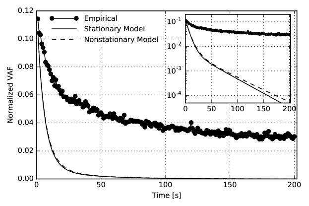
Figure 1: Empirical and theoretical VAF of KGHM (one of the most liquid stock at Warsaw Stock Exchange) in years 2011-2012 in the linear and semilogarithmic coordinates. Points are empirical result, solid line represents stationary model and dashed line nonstationary model (see section 5). Both approaches do not fit empirical data. Fitted values of the parameters are: $M=0.269,$ $\epsilon=0.258,$ $\tau_{1}=3.63,$ $\tau_{2}=32.57,$ $w=0.586,$ $p=14986,$ $q=2.25\cdot 10^{8}.$

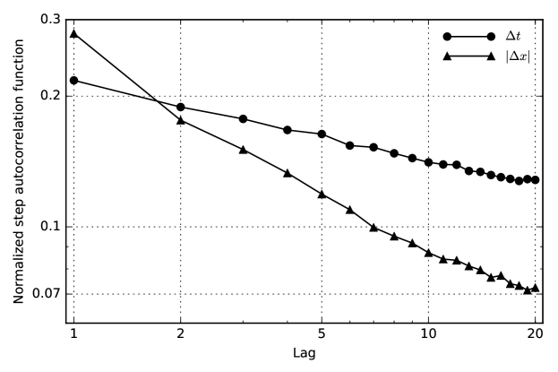
Figure 2: Normalized step autocorrelation function of waiting times and the modules of price changes for KGHM in years 2011-2012 in the logarithmic coordinates.

5 Nonstationarity

Varying mean inter-trade time during trading session is a stylized fact observed on stock prices on every market RCont2001 ; Hasbrouck2007 ; DacorognaGencayMullerOlsenPictet2001 . This intra-day pattern, often called the ”lunch effect”, is characterized by low volatility and long inter-trade times in the middle of the day. On the contrary, activity on the stock market is higher at the beginning and the end of a trading session. This effect influences the VAF of the process, as described in MWilinski , where the general formula for the impact of this phenomenon is given. Following MWilinski we describe the daily pattern with the rational function

$$\theta(t)=\frac{1}{a[(t-p)^{2}+q]},$$ (21)

where $\theta(t)$ can be interpreted as varying mean of the waiting times distribution during a trading session. Now, we can obtain an explicit expression for normalized VAF taking the seasonality into account:

$$\begin{split}C^{n}(t)&=\sum_{j=0}^{2}A_{j}Jv_{j}^{-\frac{1}{2}}e^{-v_{j}\tau_{min}}\left[\text{erf}\left(\sqrt{v_{j}J_{0}}\right)+\text{erf}\left(\sqrt{v_{j}J_{k}}\right)\right],\\ J&=\frac{1}{2(T-t)}\sqrt{\frac{\pi X}{t}},\\ J_{0}&=\frac{t}{X}\left(\frac{t}{2}-p\right)^{2},\\ J_{k}&=\frac{t}{X}\left(\frac{t}{2}-(p-T)\right)^{2},\\ \tau_{min}&=\dfrac{\frac{t^{2}}{12}+q}{X}t,\\ X&=\frac{T^{2}}{3}-pT+p^{2}+q,\end{split}$$ (22)

where $T$ is the length of a day, parameters $p$ and $q$ are fitted to data and come from the rational form of day seasonality and erf is the error function. As shown in Fig. 1, taking nonstationarity into account slightly improves the results. However, considering the day seasonality is not enough to explain empirical VAF for jump modules.

6 Conclusions

We proposed and solved Directed CTRW model with one-step memory in jumps and obtained the analytical equation for propagator, first two moments and velocity autocorrelation function (20). Obtained VAF shows interesting properties: it is positive; it decays exponentially but slower than the VAF for the non-directed process; VAF can be nonzero even without any memory ($\epsilon=0$) for non-exponential WTD. Next, we considered nonstationarity in the form of rational function (21) and obtained analytical VAF (22).

Presented simple model, despite being analytically solvable, turned out to be unable to describe empirical data. This result suggests that simple bid-ask bounce phenomenon is not sufficient to explain long memory in financial time series and volatility clustering. We suggest that taking into account at least one of the existing long memories in jumps modules or waiting times (see Fig. 2) would improve the results.

References

- [1] E. W. Montroll and G. H. Weiss. Random walks on lattices. II. Journal of Mathematical Physics, 6(2):167–181, 1965.
- [2] Ryszard Kutner and Jaume Masoliver. The continuous time random walk, still trendy: fifty-year history, state of art and outlook. The European Physical Journal B, 90(3):50, Mar 2017.
- [3] H. Scher and E. W. Montroll. Anomalous transit-time dispersion in amorphous solids. Physical Review B, 12(6):2455–2477, Sep 1975.
- [4] G. Pfister and H. Scher. Dispersive (non-gaussian) transient transport in disordered solids. Advances in Physics, 27(5):747–798, 1978.
- [5] E. W. Montroll and M. F. Schlesinger. On the wonderful world of random walks. In J. Lebowitz and E.M. Montroll, editors, Nonequilibrium Phenomena II. From Stochastics to Hydrodynamics, pages 1–121. North-Holland, Amsterdam, 1984.
- [6] G.H. Weiss. A primer of random walkology. In Fractals in Science, pages 119–162. Springer, 1994.
- [7] J.-P. Bouchaud and A. Georges. Anomalous diffusion in disordered media: statistical mechanisms, models and physical applications. Physics Reports, 195(4):127–293, 1990.
- [8] D. Ben-Avraham and S. Havlin. Diffusion and reactions in fractals and disordered systems. Cambridge University Press, 2000.
- [9] R. Hilfer. On fractional diffusion and continuous time random walks. Physica A: Statistical Mechanics and its Applications, 329(1):35 – 40, 2003.
- [10] E. Barkai and Y.-Ch. Cheng. Aging continuous time random walks. The Journal of Chemical Physics, 118(14):6167–6178, 2003.
- [11] C. Monthus and J.-P. Bouchaud. Models of traps and glass phenomenology. Journal of Physics A: Mathematical and General, 29(14):3847, 1996.
- [12] W. Dieterich and P. Maass. Constant dielectric loss in disordered ionic conductors: Theoretical aspects. Solid State Ionics, 180(6):446–450, 2009.
- [13] N. Iyengar, C.K. Peng, R. Morin, A.L. Goldberger, and L.A. Lipsitz. Age-related alterations in the fractal scaling of cardiac interbeat interval dynamics. American Journal of Physiology-Regulatory, Integrative and Comparative Physiology, 271(4):R1078–R1084, 1996.
- [14] J. Nelson. Continuous-time random-walk model of electron transport in nanocrystalline TiO2 electrodes. Physical Review B, 59(23):15374, 1999.
- [15] M.A. Lomholt, K. Tal, R. Metzler, and J. Klafter. Lévy strategies in intermittent search processes are advantageous. Proceedings of the National Academy of Sciences, 105(32):11055–11059, 2008.
- [16] G. Margolin and B. Berkowitz. Application of continuous time random walks to transport in porous media. The Journal of Physical Chemistry B, 104(16):3942–3947, 2000.
- [17] A. Helmstetter and D. Sornette. Diffusion of epicenters of earthquake aftershocks, Omori’s law, and generalized continuous-time random walk models. Physical Review E, 66(6):061104, 2002.
- [18] H. Scher, G. Margolin, R. Metzler, J. Klafter, and B. Berkowitz. The dynamical foundation of fractal stream chemistry: The origin of extremely long retention times. Geophysical Research Letters, 29(5):5–1, 2002.
- [19] R. Hempelmann. Hydrogen diffusion in proton conducting oxides and in nanocrystalline metals. In R. Kutner, A. Pȩkalski, and K. Sznajd-Weron, editors, Anomalous Diffusion From Basics to Applications, pages 247–252. Springer, 1999.
- [20] L. Hufnagel, D. Brockmann, and T. Geisel. The scaling laws of human travel. Nature, 439:462–465, 2006.
- [21] E. Scalas, R. Gorenflo, and F. Mainardi. Fractional calculus and continuous-time finance. Physica A: Statistical Mechanics and its Applications, 284(1-4):376 – 384, 2000.
- [22] F. Mainardi, M. Raberto, R. Gorenflo, and E. Scalas. Fractional calculus and continuous-time finance ii: the waiting-time distribution. Physica A: Statistical Mechanics and its Applications, 287(3-4):468 – 481, 2000.
- [23] M. Raberto, E. Scalas, and F. Mainardi. Waiting-times and returns in high-frequency financial data: an empirical study. Physica A: Statistical Mechanics and its Applications, 314(1-4):749 – 755, 2002.
- [24] E. Scalas, R. Gorenflo, and F. Mainardi. Uncoupled continuous-time random walks: Solution and limiting behavior of the master equation. Physical Review E, 69(1):011107, 2004.
- [25] E. Scalas. The application of continuous-time random walks in finance and economics. Physica A: Statistical Mechanics and its Applications, 362(2):225 – 239, 2006.
- [26] R. Kutner and F. Świtała. Stochastic simulations of time series within Weierstrass - Mandelbrot walks. Quantitative Finance, 3(3):201–211, 2003.
- [27] J. Masoliver, M. Montero, and G. H. Weiss. Continuous-time random-walk model for financial distributions. Physical Review E, 67(2):021112, 2003.
- [28] P. Repetowicz and P. Richmond. Modeling share price evolution as a continuous time random walk (ctrw) with non-independent price changes and waiting times. Physica A: Statistical Mechanics and its Applications, 344(1-2):108 – 111, 2004. Applications of Physics in Financial Analysis 4 (APFA4).
- [29] J. Masoliver, M. Montero, J. Perelló, and G. H. Weiss. The continuous time random walk formalism in financial markets. Journal of Economic Behavior Organization, 61(4):577–598, 2006.
- [30] J. Masoliver, M. Montero, J. Perello, and G. H. Weiss. The CTRW in finance: Direct and inverse problems with some generalizations and extensions. Physica A: Statistical Mechanics and its Applications, 379(1):151 – 167, 2007.
- [31] R. Kutner. Stock market context of the lévy walks with varying velocity. Physica A: Statistical Mechanics and its Applications, 314(1):786–795, 2002.
- [32] E. Scalas. Five years of continuous-time random walks in econophysics. In The Complex Networks of Economic Interactions, pages 3–16. Springer, 2006.
- [33] J. Perelló, J. Masoliver, A. Kasprzak, and R. Kutner. Model for interevent times with long tails and multifractality in human communications: An application to financial trading. Physical Review E, 78(3):036108, 2008.
- [34] Tomasz Gubiec and Ryszard Kutner. Continuous-time random walk with multi-step memory: an application to market dynamics. The European Physical Journal B, 90(11):228, Nov 2017.
- [35] Tomasz Gubiec and Ryszard Kutner. Backward jump continuous-time random walk: An application to market trading. Phys. Rev. E, 82:046119, Oct 2010.
- [36] A. Kasprzak, R. Kutner, J. Perelló, and J. Masoliver. Higher-order phase transitions on financial markets. The European Physical Journal B, 76(4):513–527, 2010.
- [37] R. Metzler and J. Klafter. The random walk’s guide to anomalous diffusion: a fractional dynamics approach. Physics Reports, 339(1):1–77, 2000.
- [38] H. Scher, M. F. Shlesinger, and J. T. Bendler. Time-scale invariance in transport and relaxation. Physics Today, 44:26–34, January 1991.
- [39] J. W. Haus and K. W. Kehr. Diffusion in regular and disordered lattices. Physics Reports, 150(5-6):263 – 406, 1987.
- [40] K.W. Kehr, R. Kutner, and K. Binder. Diffusion in concentrated lattice gases. self-diffusion of noninteracting particles in three-dimensional lattices. Physical Review B, 23(10):4931–4945, 1981.
- [41] R. Kutner. Correlated hopping in honeycomb lattice: tracer diffusion coefficient at arbitrary lattice gas concentration. Journal of Physics C: Solid State Physics, 18(34):6323, 1985.
- [42] T. Gubiec and R. Kutner. Share price evolution as stationary, dependent continuous-time random walk. Acta Physica Polonica, A, 117(4):669 – 672, 2010.
- [43] M. Montero and J. Masoliver. Nonindependent continuous-time random walks. Physical Review E, 76(6):061115, 2007.
- [44] M. Montero Torralbo. Parrondo-like behavior in continuous-time random walks with memory. Physical Review E, 84:051139, 2011.
- [45] Vincent Tejedor and Ralf Metzler. Anomalous diffusion in correlated continuous time random walks. Journal of Physics A: Mathematical and Theoretical, 43(8):082002, 2010.
- [46] Marcin Magdziarz, Ralf Metzler, Wladyslaw Szczotka, and Piotr Zebrowski. Correlated continuous-time random walks in external force fields. Phys. Rev. E, 85:051103, May 2012.
- [47] Aleksei V. Chechkin, Michael Hofmann, and Igor M. Sokolov. Continuous-time random walk with correlated waiting times. Phys. Rev. E, 80:031112, Sep 2009.
- [48] Jae-Hyung Jeon, Natascha Leijnse, Lene B Oddershede, and Ralf Metzler. Anomalous diffusion and power-law relaxation of the time averaged mean squared displacement in worm-like micellar solutions. New Journal of Physics, 15(4):045011, 2013.
- [49] Ruey S. Tsay. Analysis of financial time series. Wiley series in probability and statistics. Wiley-Interscience, Hoboken, NJ, 2. ed. edition, 2005.
- [50] R. Cont. Empirical properties of asset returns: stylized facts and statistical issues. Quantitative Finance, 1(2):223–236, 2001.
- [51] Rama Cont. Long range dependence in financial markets. In Jacques Lévy-Véhel and Evelyne Lutton, editors, Fractals in Engineering, pages 159–179, London, 2005. Springer London.
- [52] J. K. E. Tunaley. Theory of ac conductivity based on random walks. Physical Review Letters, 33(17):1037–1039, 1974.
- [53] J. K. E. Tunaley. Asymptotic solutions of the continuous-time random walk model of diffusion. Journal of Statistical Physics, 11:397–408, 1974.
- [54] T. Gubiec and M. Wiliďż˝ski. Intra-day variability of the stock market activity versus stationarity of the financial time series. Physica A: Statistical Mechanics and its Applications, 432:216 – 221, 2015.
- [55] Joel Hasbrouck. Empirical Market Microstructure: The Institutions, Economics, and Econometrics of Securities Trading. Oxford University Press, 2007.
- [56] M. M. Dacorogna, R. Gencay, U. Muller, R. B. Olsen, and O. V. Pictet. An introduction to high frequency finance. Academic Press, New York, 2001.