A multiscale neural network based on hierarchical matrices

Abstract

In this work we introduce a new multiscale artificial neural network based on the structure of $\mathcal{H}$-matrices. This network generalizes the latter to the nonlinear case by introducing a local deep neural network at each spatial scale. Numerical results indicate that the network is able to efficiently approximate discrete nonlinear maps obtained from discretized nonlinear partial differential equations, such as those arising from nonlinear Schrödinger equations and the Kohn-Sham density functional theory.

Keywords: $\mathcal{H}$-matrix; multiscale neural network; locally connected neural network; convolutional neural network

1 Introduction

In the past decades, there has been a great combined effort in developing efficient algorithms to solve linear problems issued from discretization of integral equations (IEs), and partial differential equations (PDEs). In particular, multiscale methods such as multi-grid methods [10], the fast multipole method [21], wavelets [46], and hierarchical matrices [9, 23], have been strikingly successful in reducing the complexity for solving such systems. In several cases, for operators of pseudo-differential type, these algorithms can achieve linear or quasi-linear complexity. In a nutshell, these methods aim to use the inherent multiscale structure of the underlying physical problem to build efficient representations at each scale, thus compressing the information contained in the system. The gains in complexity stem mainly from processing information at each scale, and merging it in a hierarchical fashion.

Even though these techniques have been extensively applied to linear problems with outstanding success, their application to nonlinear problems has been, to the best of our knowledge, very limited. This is due to the high complexity of the solution maps. In particular, building a global approximation of such maps would normally require an extremely large amount of parameters, which in return, is often translated to algorithms with a prohibitive computational cost. The development of algorithms and heuristics to reduce the cost is an area of active research [6, 18, 17, 22, 45]. However, in general, each method is application-dependent, and requires a deep understanding of the underlying physics.

On the other hand, the surge of interest in machine learning methods, in particular, deep neural networks, has dramatically improved speech recognition [30], visual object recognition [37], object detection, etc. This has fueled breakthroughs in many domains such as drug discovery [44], genomics [39], and automatic translation [57], among many others [38, 55]. Deep neural networks have empirically shown that it is possible to obtain efficient representations of very high-dimensional functions. Even though the universality theorem holds for neural networks [15, 32, 34, 48], i.e., they can approximate arbitrarily well any function with mild regularity conditions, how to efficiently build such approximations remains an open question. In particular, the degree of approximation depends dramatically on the architecture of the neural network, i.e. how the different layers are connected. In addition, there is a fine balance between the number of parameters, the architecture, and the degree of approximation [27, 28, 48].

This paper aims to combine the tools developed in deep neural networks with ideas from multiscale methods. In particular, we extend hierarchical matrices ($\mathcal{H}$-matrices) to nonlinear problems within the framework of neural networks. Let

$$u=\mathcal{M}(v),\quad u,v\in\Omega\subset\mathbb{R}^{n},$$ (1.1)

be a nonlinear generalization of pseudo-differential operators, issued from an underlying physical problem, described by either an integral equation or a partial differential equation, where $v$ can be considered as a parameter in the equation, $u$ is either the solution of the equation or a function of it, and $n$ is the number of variables.

We build a neural network with a novel multiscale structure inspired by hierarchical matrices. We interpret the application of an $\mathcal{H}$-matrix to a vector using a neural network structure as follows. We first reduce the dimensionality of the vector, or restrict it, by multiplying it by a short and wide structured matrix. Then we process the encoded vector by multiplying it by a structured square matrix. Then we return the vector to its original size, or interpolate it, by multiplying it by a structured tall and skinny matrix. Such operations are performed separately at different spatial scales. The final approximation to the matrix-vector multiplication is obtained by adding the contributions from all spatial scales, including the near-field contribution, which is represented by a near-diagonal matrix. Since every step is linear, the overall operation is also a linear mapping. This interpretation allows us to directly generalize the $\mathcal{H}$-matrix to nonlinear problems by replacing the structured square matrix in the processing stage by a structured nonlinear network with several layers. The resulting artificial neural network, which we call multiscale neural network, only requires a relatively modest amount of parameters even for large problems.

We demonstrate the performance of the multiscale neural network by approximating the solution to the nonlinear Schrödinger equation [2, 51], as well as the Kohn-Sham map [31, 36]. These mappings are highly nonlinear, and are still well approximated by the proposed neural network, with a relative accuracy on the order of $10^{-4}\sim 10^{-3}$. Furthermore, we do not observe overfitting even in the presence of a relatively small set of training samples.

1.1 Related work

Although machine learning and deep learning literature is vast, the application of deep learning to numerical analysis problems is relatively new, though that is rapidly changing. Research using deep neural networks with multiscale architectures has primarily focused on image [4, 11, 13, 42, 53, 60] and video [47] processing.

Deep neural networks have been recently used to solve PDEs [7, 8, 12, 16, 26, 40, 43, 54, 56] and classical inverse problems [3, 49]. For general applications of machine learning to nonlinear numerical analysis problems, the work of Raissi and Karnidiakis used machine learning, in particular, Gaussian processes, to find parameters in nonlinear equations [52]; Chan, and Elsheikh predicted the basis function on the coarse grid in multiscale finite volume method by neural network; Khoo, Lu and Ying used neural network in the context of uncertainty quantification [33]; Zhang et al used neural network in the context of generating high-quality interatomic potentials for molecular dynamics [64, 65]. Wang et al. applied non-local multi-continuum neural network on time-dependent nonlinear problems [61]. Khrulkov et al. and Cohen et al. developed deep neural network architectures based on tensor-train decomposition [15, 34]. In addition, we note that deep neural networks with related multi-scale structures [53, 50] have been proposed mainly for applications such as image processing, however, we are not aware of any applications of such architectures to solving nonlinear differential or integral equations.

1.2 Organization

The reminder of the paper is organized as follows. Section 2 reviews the $\mathcal{H}$-matrices and interprets the $\mathcal{H}$-matrices using the framework of neural networks. Section 3 extends the neural network representation of $\mathcal{H}$-matrices to the nonlinear case. Section 4 discusses the implementation details and demonstrates the accuracy of the architecture in representing nonlinear maps, followed by the conclusion and future directions in Section 5.

2 Neural network architecture for $\mathcal{H}$-matrices

In this section, we aim to represent the matrix-vector multiplication of $\mathcal{H}$-matrices within the framework of neural networks. For the sake of clarity, we succinctly review the structure of $\mathcal{H}$-matrices for the one dimensional case in Section 2.1. We interpret $\mathcal{H}$-matrices using the framework of neural networks in Section 2.2, and then extend it to the multi-dimensional case in Section 2.3.

2.1 $\mathcal{H}$-matrices

Hierarchical matrices ($\mathcal{H}$-matrices) were first introduced by Hackbusch et al. in a series of papers [23, 25, 24] as an algebraic framework for representing matrices with a hierarchically off-diagonal low-rank structure. This framework provides efficient numerical methods for solving linear systems arising from integral equations (IE) and partial differential equations (PDE) [9]. In the sequel, we follow the notation in [41] to provide a brief introduction to the framework of $\mathcal{H}$-matrices in a simple uniform and Cartesian setting. The interested readers are referred to [23, 9, 41] for further details.

Consider the integral equation

$$u(x)=\int_{\Omega}g(x,y)v(y)\,\mathrm{d}y,\quad\Omega=[0,1),$$ (2.1)

where $u$ and $v$ are periodic in $\Omega$ and $g(x,y)$ is smooth and numerically low-rank away from the diagonal. A discretization with an uniform grid with $N=2^{L}m$ discretization points yields the linear system given by

$$u=Av,$$ (2.2)

where $A\in\mathbb{R}^{N\times N}$, and $u,v\in\mathbb{R}^{N}$ are the discrete analogues of $u(x)$ and $v(x)$ respectively.

We introduce a hierarchical dyadic decomposition of the grid in $L+1$ levels as follows. We start by the $0$-th level of the decomposition, which corresponds to the set of all grid points defined as

$$\mathcal{I}^{(0)}=\{k/N:k=0,\dots,N-1\}.$$ (2.3)

At each level $\ell$ ($0\leq\ell\leq L$), we decompose the grid in $2^{\ell}$ disjoint segments.

Each segment is defined by $\mathcal{I}^{(\ell)}_{i}=\mathcal{I}^{(0)}\cap[(i-1)/2^{\ell},i/2^{\ell})$ for $i=1,\dots,2^{\ell}$. Throughout this manuscript, $\mathcal{I}^{(\ell)}$(or $\mathcal{J}^{(\ell)}$) denote a generic segment of a given level $\ell$, and the superscript $\ell$ will be omitted when the level is clear from the context. Moreover, following the usual terminology in $\mathcal{H}$-matrices, we say that a segment $\mathcal{J}^{(l)}$ ($\ell\geq 1$) is the parent of a segment $\mathcal{I}^{(l-1)}$ if $\mathcal{I}^{(l-1)}\subset\mathcal{J}^{(l)}$. Symmetrically, $\mathcal{I}^{(l-1)}$ is called a child of $\mathcal{J}^{(l)}$. Clearly, each segment, except those on level $L$, have two child segments.

Figure 1: Illustration of the computational domain at level $\ell=2,3,4$. The left and right figures represent an interior segment and a boundary segment and their adjacent and interaction list at different levels.

In addition, for a segment $\mathcal{I}$ on level $\ell\geq 2$, we define the following lists:

• neighbor list of $\mathcal{I}$. List of the segments on level $\ell$ that are adjacent to $\mathcal{I}$ including $\mathcal{I}$ itself;

• interaction list of $\mathcal{I}$. If $\ell=2$, $\mathsf{IL}(\mathcal{I})$ contains all the segments on level $2$ minus $\mathsf{NL}(\mathcal{I})$. If $\ell>2$, $\mathsf{IL}(\mathcal{I})$ contains all the segments on level $\ell$ that are children of segments in $\mathsf{NL}(\mathcal{P})$ with $\mathcal{P}$ being $\mathcal{I}$’s parent minus $\mathsf{NL}(\mathcal{I})$.

Fig. 1 illustrates the dyadic partition of the computational domain and the lists on levels $\ell=2,3,4$. Clearly, $\mathcal{J}\in\mathsf{NL}(\mathcal{I})$ if and only if $\mathcal{I}\in\mathsf{NL}(\mathcal{J})$, and $\mathcal{J}\in\mathsf{IL}(\mathcal{I})$ if and only if $\mathcal{I}\in\mathsf{IL}(\mathcal{J})$.

Figure 2: Partition of the matrix $A$ for $L=4$ and nonzero blocks of $A^{(\ell)}$, $\ell=2,3,4$ (colored blue) and $A^{(\mathrm{ad})}$ (colored orange). Nonzero blocks of $A^{(\ell)}$ are approximated by low rank approximation and nonzero blocks of $A^{(\mathrm{ad})}$ are retained.

For a vector $v\in\mathbb{R}^{N}$, $v_{\mathcal{I}}$ denotes the elements of $v$ indexed by $\mathcal{I}$ and for a matrix $A\in\mathbb{R}^{N\times N}$, $A_{\mathcal{I},\mathcal{J}}$ represents the submatrix given by the elements of $A$ indexed by $\mathcal{I}\times\mathcal{J}$. The dyadic partition of the grid and the interaction lists induce a multilevel decomposition of $A$ as follows

$$A=\sum_{\ell=2}^{L}A^{(\ell)}+A^{(\mathrm{ad})},\qquad\begin{aligned} A^{(\ell)}_{\mathcal{I},\mathcal{J}}&=\begin{cases}A_{\mathcal{I},\mathcal{J}},&\mathcal{I}\in\mathsf{IL}(\mathcal{J});\\ 0,&\text{otherwise},\end{cases}\mathcal{I},\mathcal{J}\text{ at level }\ell,2\leq\ell\leq L,\\ A^{(\mathrm{ad})}_{\mathcal{I},\mathcal{J}}&=\begin{cases}A_{\mathcal{I},\mathcal{J}},&\mathcal{I}\in\mathsf{NL}(\mathcal{J});\\ 0,&\text{otherwise},\end{cases}\mathcal{I},\mathcal{J}\text{ at level }L.\end{aligned}$$ (2.4)

In a nutshell, $A^{(\ell)}$ considers the interaction at level $\ell$ between a segment and its interaction list, and $A^{(\mathrm{ad})}$ considers all the interactions between adjacent segments at level $L$.

Fig. 2 illustrates the block partition of $A$ induced by the dyadic partition, and the decomposition induced by the different interaction lists at each level that follows (2.4).

\begin{overpic}[height=75.8804pt]{Avl2.pdf} \put(-1.0,42.0){$u^{(\ell)}$} \put(15.0,42.0){$U^{(\ell)}$} \put(40.0,42.0){$M^{(\ell)}$} \put(70.0,42.0){$(V^{(\ell)})^{T}$} \put(98.0,42.0){$v$} \end{overpic}

(a) $u^{(\ell)}=A^{(\ell)}v\approx U^{(\ell)}M^{(\ell)}(V^{(\ell)})^{T}v$

\begin{overpic}[height=75.8804pt]{Avad.pdf} \put(-1.0,78.0){$u^{(\mathrm{ad})}$} \put(50.0,78.0){$A^{(\mathrm{ad})}$} \put(95.0,78.0){$v$} \end{overpic}

(b) $u^{(\mathrm{ad})}=A^{(\mathrm{ad})}v$

Figure 3: Diagram of matrix-vector multiplication (2.7) of the low-rank part and adjacent part of $\mathcal{H}$-matrices. The blocks of $M^{(\ell)}$ colored by pale orange are zero blocks, and if we treat these blocks as non-zero blocks, the matrices $M^{(\ell)}$ are block cyclic band matrices.

 

The key idea behind $\mathcal{H}$-matrices is to approximate the nonzero blocks $A^{(\ell)}$ by a low rank approximation (see [35] for a thorough review). This idea is depicted in Fig. 2, in which each non-zero block is approximated by a tall and skinny matrix, a small squared one and a short and wide one, respectively. In this work, we focus on the uniform $\mathcal{H}$-matrices [20], and, for simplicity, we suppose that each block has a fixed rank at most $r$, i.e.

$$A^{(\ell)}_{\mathcal{I},\mathcal{J}}\approx U^{(\ell)}_{\mathcal{I}}M^{(\ell)}_{\mathcal{I},\mathcal{J}}(V^{(\ell)}_{\mathcal{J}})^{T},\quad U^{(\ell)}_{\mathcal{I}},V^{(\ell)}_{\mathcal{J}}\in\mathbb{R}^{N/2^{\ell}\times r},\quad M^{(\ell)}_{\mathcal{I},\mathcal{J}}\in\mathbb{R}^{r\times r}.$$ (2.5)

where $\mathcal{I},$ and $\mathcal{J}$ are any interacting segments at level $\ell$.

The main observation is that it is possible to factorize each $A^{(\ell)}$ as $A^{(\ell)}\approx U^{(\ell)}M^{(\ell)}(V^{(\ell)})^{T}$ depicted in Fig. 3a. $U^{(\ell)}$ is a block diagonal matrix with diagonal blocks $U^{(\ell)}_{\mathcal{I}}$ for $\mathcal{I}$ at level $\ell$, $V^{(\ell)}$ is a block diagonal matrix with diagonal blocks $V^{(\ell)}_{\mathcal{J}}$ for $\mathcal{J}$ at level $\ell$, and finally $M^{(\ell)}$ aggregates all the blocks $M^{(\ell)}_{\mathcal{I},\mathcal{J}}$ for all interacting segments $\mathcal{I},\mathcal{J}$ at level $\ell$. This factorization induces a decomposition of $A$ given by

$$A=\sum_{\ell=2}^{L}A^{(\ell)}+A^{(\mathrm{ad})}\approx\sum_{\ell=2}^{L}U^{(\ell)}M^{(\ell)}(V^{(\ell)})^{T}+A^{(\mathrm{ad})}.$$ (2.6)

Thus the matrix-vector multiplication (2.2) can be expressed as

$$u \approx\sum_{\ell=2}^{L}u^{(\ell)}+u^{(\mathrm{ad})}=\sum_{\ell=2}^{L}U^{(\ell)}M^{(\ell)}(V^{(\ell)})^{T}v+A^{(\mathrm{ad})}v,$$ (2.7)

as illustrated in Fig. 3a, which constitutes the basis for writing $\mathcal{H}$-matrices as a neural network.

In addition, the matrices $\{U^{(\ell)},V^{(\ell)},M^{(\ell)}\}_{\ell=2}^{L}$ and $A^{(\mathrm{ad})}$ have the following properties.

Property 1.

The matrices

1. $U^{(\ell)}$ and $V^{(\ell)}$, $\ell=2,\cdots,L$ are block diagonal matrices with block size $N/2^{\ell}\times r$;

2. $A^{(\mathrm{ad})}$ is a block cyclic tridiagonal matrix with block size $m\times m$;

3. $M^{(\ell)}$, $\ell=2,\cdots,L$ are block cyclic band matrices with block size $r\times r$ and band size $n_{b}^{(\ell)}$, which is $2$ for $\ell=2$ and $3$ for $\ell\geq 3$, if we treat all the pale orange colored blocks of $M^{(\ell)}$ in Fig. 3a as nonzero blocks.

We point out that the band sizes $n_{b}^{(\ell)}$ and $n^{(\mathrm{ad})}_{b}$ depend on the definitions of $\mathsf{NL}$ and $\mathsf{IL}$. In this case, the list were defined using the strong admissible condition in $\mathcal{H}$-matrices. Other conditions can be certainly used, such as the weak admissibility condition, leading to similar structures.

2.2 Matrix-vector multiplication as a neural network

An artificial neural network, in particular, a feed-forward network, can be thought of the composition of several simple functions, usually called propagation functions, in which the intermediate one-dimensional variables are called neurons, which in return, are organized in vector, or tensor, variables called layers. For example, an artificial feed-forward neural network

$$u=\mathcal{F}(v),\qquad u,v\in\mathbb{R}^{n}$$ (2.8)

with $K+1$ layer can be written using the following recursive formula

$$\begin{split}\xi^{(0)}&=v,\\ \xi^{(k)}&=\phi(W^{(k)}\xi^{(k-1)}+b^{(k)}),\\ u&=\xi^{(K)},\end{split}$$ (2.9)

where for each $k=1,...,K$ we have that $\xi^{(k)},b^{(k)}\in\mathbb{R}^{n_{k}},W^{(k)}\in\mathbb{R}^{n_{k}\times n_{k-1}}$. Following the terminology of machine learning, $\phi$ is called the activation function that is applied entry-wise, $W^{(k)}$ are the weights, $b^{(k)}$ are the biases, and $\xi^{(k)}$ is the $k$-th layer containing $n_{k}$ number of neurons. Typical choices for the activation function are linear function, the rectified-linear unit (ReLU), or sigmoid function. In addition, (2.9) can easily be rewritten using tensors by replacing the matrix-vector multiplication by the more general tensor contraction. We point out that representing layers with tensors or vectors is equivalent up to reordering and reshaping. The main advantage of using the former is that layers, and its propagating functions, can be represented in a more compact fashion. Therefore, in what follows we predominantly use a tensor representation.

Within this context, training a network refers to finding the weights and biases, whose entries are collectively called parameters, in order to approximate a given map. This is usually done by minimizing a loss function using a stochastic optimization algorithm.

2.2.1 Locally connected networks

We interpret the structure of $\mathcal{H}$-matrices (2.6) using the framework of neural networks. The different factors in (2.7) possess a distinctive structure, which we aim to exploit by using locally connected (LC) network. LC networks are propagating functions whose weights have a block-banded constraint. For the one-dimensional example, we also treat $\xi$ as a 2-tensor of dimensions $\alpha\times N_{x}$, where $\alpha$ is the channel dimension and $N_{x}$ is the spatial dimension, and $\zeta$ be a 2-tensor of dimensions $\alpha^{\prime}\times N_{x}^{\prime}$. We say that $\xi$ is connected to $\zeta$ by a LC networks if

$$\zeta_{c^{\prime},i}=\phi\left(\sum_{j=(i-1)s+1}^{(i-1)s+w}\sum_{c=1}^{\alpha}W_{c^{\prime},c;i,j}\xi_{c,j}+b_{c^{\prime},i}\right),\quad i=1,\dots,N_{x}^{\prime},~{}c^{\prime}=1,\dots,\alpha^{\prime},$$ (2.10)

where $w$ and $s\in\mathbb{N}$ are the kernel window size and stride, respectively. In addition, we say that $\zeta$ is a locally connected (LC) layer if it satisfies (2.10).

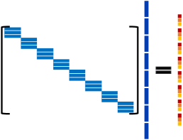
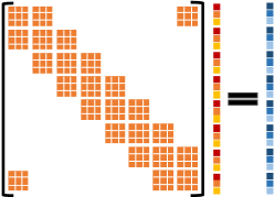
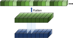
$s=w=\frac{N_{x}}{N_{x}^{\prime}}$, $\alpha=1$	$s=1$, $N_{x}^{\prime}=N_{x}$	$s=1$, $w=1$, $N_{x}^{\prime}=N_{x}$
(a) $\mathsf{LCR}[\phi;N_{x},N_{x}^{\prime},\alpha^{\prime}]$ with $N_{x}=32$, $N_{x}^{\prime}=8$ and $\alpha^{\prime}=3$	(b) $\mathsf{LCK}[\phi;N_{x},\alpha,\alpha^{\prime},w]$ with $N_{x}=8$, $\alpha=\alpha^{\prime}=3$ and $w=3$	(c) $\mathsf{LCI}[\phi;N_{x},\alpha,\alpha^{\prime}]$ with $N_{x}=8$, $\alpha=3$ and $\alpha^{\prime}=4$

Figure 4: Three instances of locally connected networks used the represent the matrix-vector multiplication in (2.7). The upper portions of each column depicts the patterns of the matrices and the lower portions are their respective analogues using locally connect networks.

Each LC network requires $6$ parameters, $N_{x}$, $\alpha$, $N_{x}^{\prime}$, $\alpha^{\prime}$, $w$ and $s$ to be characterized. Next, we define three types of LC network by specifying some of their parameters,

• Restriction network: we set $s=w=\frac{N_{x}}{N_{x}^{\prime}}$ and $\alpha=1$ in LC. This network represents the multiplication of a block diagonal matrix with block sizes $\alpha^{\prime}\times s$ and a vector with size $N_{x}\alpha$, as illustrated by Fig. 4 (a). We denote this network using $\mathsf{LCR}[\phi;N_{x},N_{x}^{\prime},\alpha^{\prime}]$. The application of $\mathsf{LCR}[\mathsf{linear};32,8,3]$ is depicted in Fig. 4 (a).

• Kernel network: we set $s=1$ and $N_{x}^{\prime}=N_{x}$. This network represents the multiplication of a cyclic block band matrix of block size $\alpha^{\prime}\times\alpha$ and band size $\frac{w-1}{2}$ times a vector of size $N_{x}\alpha$, as illustrated by the upper portion of Fig. 4 (b). To account for the periodicity we pad the input layer $\xi_{c,j}$ on the spatial dimension to the size $(N_{x}+w-1)\times\alpha$. We denote this network by $\mathsf{LCK}[\phi;N_{x},\alpha,\alpha^{\prime},w]$. This network has two steps: the periodic padding of $\xi_{c,j}$ on the spatial dimension, and the application of (2.10). The application of $\mathsf{LCK}[\mathsf{linear};8,3,3,3]$ is depicted in Fig. 4 (b).

• Interpolation network: we set $s=w=1$ and $N_{x}^{\prime}=N_{x}$ in LC. This network represents the multiplication of a block diagonal matrix with block size $\alpha^{\prime}\times\alpha$, times a vector of size $N_{x}\alpha$, as illustrated by the upper figure in Fig. 4 (c). We denote the network $\mathsf{LCI}[\phi;N_{x},\alpha,\alpha^{\prime}]$, which has two steps: the application of (2.10), and the reshaping of the output to a vector by column major indexing. The application of $\mathsf{LCI}[\mathsf{linear};8,3,4]$ is depicted in Fig. 4 (c).

2.2.2 Neural network representation

Following (2.7), in order to construct the neural network (NN) architecture for (2.7), we need to represent the following four operations:

$$\xi^{(\ell)} =(V^{(\ell)})^{T}v,$$ (2.11a)

$$\zeta^{(\ell)} =M^{(\ell)}\xi^{(\ell)},$$ (2.11b)

$$u^{(\ell)} =U^{(\ell)}\zeta^{(\ell)},$$ (2.11c)

$$u^{(\mathrm{ad})} =A^{(\mathrm{ad})}v.$$ (2.11d)

From 1.1 and the definition of $\mathsf{LCR}$ and $\mathsf{LCI}$, the operations (2.11a) and (2.11c) are equivalent to

$$\xi^{(\ell)}=\mathsf{LCR}[\mathsf{linear};N,2^{\ell},r](v),\quad u^{(\ell)}=\mathsf{LCI}[\mathsf{linear};2^{\ell},r,\frac{N}{2^{\ell}}](\zeta^{(\ell)}),$$ (2.12)

respectively. Analogously, 1.3 indicates that (2.11b) is equivalent to

$$\zeta^{(\ell)}=\mathsf{LCK}[\mathsf{linear};2^{\ell},r,r,2n_{b}^{(\ell)}+1](\xi^{(\ell)}).$$ (2.13)

We point out that $\xi^{(\ell)}$ is a vector in (2.11c) but a $2$-tensor in (2.12) and (2.13). In principle, we need to flatten $\xi^{(\ell)}$ in (2.12) to a vector and reshape it back to a 2-tensor before (2.13). These operations do not alter the algorithmic pipeline, so they are omitted.

Given that $v,u^{(\mathrm{ad})}$ are vectors, but $\mathsf{LCK}$ is defined for 2-tensors, we explicitly write the reshape and flatten operations. Denote as $\mathsf{Reshape}[n_{1},n_{2}]$ the map that reshapes a vector of size $n_{1}n_{2}$ into a 2-tensor of size $n_{1}\times n_{2}$ by column major indexing, and $\mathsf{Flatten}$ is defined as the inverse of $\mathsf{Reshape}$. Using 1.2, we can write (2.11d) as

$$\tilde{v}=\mathsf{Reshape}[m,2^{L}](v),~{}\tilde{u}^{(\mathrm{ad})}=\mathsf{LCK}\left[\mathsf{linear};2^{L},m,m,2n^{(\mathrm{ad})}_{b}+1\right](\tilde{v}),~{}u^{(\mathrm{ad})}=\mathsf{Flatten}(\tilde{u}^{(\mathrm{ad})}).$$ (2.14)

\begin{overpic}[width=390.25534pt]{hnnlinear.pdf} \put(17.3,13.7){\tiny$\mathsf{LCR}$-$\mathsf{linear}$} \put(17.3,19.7){\tiny$\mathsf{LCK}$-$\mathsf{linear}$} \put(17.3,25.7){\tiny$\mathsf{LCI}$-$\mathsf{linear}$} \put(57.3,13.7){\tiny$\mathsf{LCR}$-$\mathsf{linear}$} \put(57.3,19.7){\tiny$\mathsf{LCK}$-$\mathsf{linear}$} \put(57.3,25.7){\tiny$\mathsf{LCI}$-$\mathsf{linear}$} \put(89.3,22.7){\tiny$\mathsf{LCK}$-$\mathsf{linear}$} \put(84.8,30.7){\tiny$\mathsf{Flatten}$} \put(84.8,14.4){\tiny$\mathsf{Reshape}$} \put(52.5,32.3){\tiny$\mathsf{Flatten}$} \put(16.5,32.5){\tiny$\mathsf{Flatten}$} \put(53.2,44.8){\small$\mathsf{sum}$} \end{overpic}

Figure 5: Neural network architecture for $\mathcal{H}$-matrices.

Combining (2.12), (2.13) and (2.14), we obtain Algorithm 1, whose architecture is illustrated in Fig. 5. In particular, Fig. 5 is the translation to the neural network framework of (2.7) (see Fig. 3a) using the building blocks depicted in Fig. 4.

1:  u = 0;

2:  for $\ell=2$ to $L$ do

3:     $\xi=\mathsf{LCR}[\mathsf{linear};N,2^{\ell},r](v)$;

4:     $\zeta=\mathsf{LCK}[\mathsf{linear};2^{\ell},r,r,2n_{b}^{(\ell)}+1](\xi)$;

5:     $u=u+\mathsf{LCI}[\mathsf{linear};2^{\ell},r,\frac{N}{2^{\ell}}](\zeta)$;

6:  end for

7:  $\tilde{v}=\mathsf{Reshape}[m,2^{L}](v)$;

8:  $\tilde{u}^{(\mathrm{ad})}=\mathsf{LCK}\left[\mathsf{linear};2^{L},m,m,2n^{(\mathrm{ad})}_{b}+1\right](\tilde{v})$;

9:  $u^{(\mathrm{ad})}=\mathsf{Flatten}(\tilde{u}^{(\mathrm{ad})})$;

10:  $u=u+u^{(\mathrm{ad})}$;

Algorithm 1 Application of the NN representation of an $\mathcal{H}$-matrix to a vector $v\in\mathbb{R}^{N}$.

Moreover, the memory footprints of the neural network architecture and $\mathcal{H}$-matrices are asymptotically the same with respect the spatial dimension of $u$ and $v$. This can be readily shown by computing the total number of parameters. For the sake of simplicity, we only count the parameters in the weights, ignoring those in the biases. A direct calculation yields the number of parameters in $\mathsf{LCR}$, $\mathsf{LCK}$ and $\mathsf{LCI}$:

$$N_{p}^{\mathsf{LCR}}=N_{x}\alpha^{\prime},\quad N_{p}^{\mathsf{LCK}}=N_{x}\alpha\alpha^{\prime}w,\quad N_{p}^{\mathsf{LCI}}=N_{x}\alpha\alpha^{\prime},$$ (2.15)

respectively. Hence, the number of parameters in Algorithm 1 is

$$N_{p}^{\mathcal{H}} =\sum_{\ell=2}^{L}\left(Nr+2^{\ell}r^{2}(2n_{b}^{(\ell)}+1)+2^{\ell}r\frac{N}{2^{\ell}}\right)+2^{L}m^{2}(2n^{(\mathrm{ad})}_{b}+1)$$ (2.16)

$$\leq 2LNr+2^{L+1}r^{2}(2\max_{\ell=2}^{L}n_{b}^{(\ell)}+1)+Nm(2n^{(\mathrm{ad})}_{b}+1)$$

$$\leq 2N\log(N)r+3Nm(2n_{b}+1)\sim O(N\log(N)),$$

where $n_{b}=\max(n^{(\mathrm{ad})}_{b},n_{b}^{(\ell)},\ell=2,\cdots,L)$, and $r\leq m$ is used.

2.3 Multi-dimensional case

Following the previous section, the extension of Algorithm 1 to the $d$-dimensional case can be easily deduced using the tensor product of one-dimensional cases. Consider $d=2$ below for instance, and the generalization to higher dimensional case will be straight-forward. Suppose that we have an IE in 2D given by

$$u(x)=\int_{\Omega}g(x,y)v(y)\,\mathrm{d}y,\quad\Omega=[0,1)\times[0,1),$$ (2.17)

we discretize the domain $\Omega$ with a uniform grid with $n=N^{2}$ ($N=2^{L}m$) discretization points, and let $A$ be the resulting matrix obtained from discretizing (2.17). We denote the set of all grid points as

$$\mathcal{I}^{(d,0)}=\{(k_{1}/N,k_{2}/N):k_{1},k_{2}=0,\dots,N-1\}.$$ (2.18)

Clearly $\mathcal{I}^{(d,0)}=\mathcal{I}^{(0)}\otimes\mathcal{I}^{(0)}$, where $\mathcal{I}^{(0)}$ is defined in (2.3), and $\otimes$ is tensor product. At each level $\ell$ ($0\leq\ell\leq L$), we decompose the grid in $4^{l}$ disjoint boxes as $\mathcal{I}_{i}^{(d,\ell)}=\mathcal{I}_{i_{1}}^{(\ell)}\otimes\mathcal{I}_{i_{2}}^{(\ell)}$ for $i_{1},i_{2}=1,\dots,2^{l}$. The definition of the lists $\mathsf{NL}$ and $\mathsf{IL}$ can be easily extended. For each box $\mathcal{I}$, $\mathsf{NL}(\mathcal{I})$ contains $3$ boxes for 1D case, $3^{2}$ boxes for 2D case. Similarly, the decomposition (2.4) on the matrix $A$ can easily to extended for this case. Following the structure of $\mathcal{H}$-matrices, the off-diagonal blocks of $A^{(\ell)}$ can be approximated as

$$A^{(\ell)}_{\mathcal{I},\mathcal{J}}\approx U^{(\ell)}_{\mathcal{I}}M^{(\ell)}_{\mathcal{I},\mathcal{J}}(V^{(\ell)}_{\mathcal{J}})^{T},\quad\mathcal{I},\mathcal{J}\in\mathcal{I}^{(\ell)},\quad U^{(\ell)}_{\mathcal{I}},V^{(\ell)}_{\mathcal{J}}\in\mathbb{R}^{(N/2^{\ell})^{2}\times r},M^{(\ell)}_{\mathcal{I},\mathcal{J}}\in\mathbb{R}^{r\times r}.$$ (2.19)

As mentioned before, we can describe the network using tensor or vectors. In what follows we will switch between representations in order to illustrate the concepts in a compact fashion. We denote an entry of a tensor $T$ by $T_{i,j}$, where $i$ is $2$-dimensional index $i=(i_{1},i_{2})$. Using the tensor notations, $U^{(\ell)}$, $V^{(\ell)}$ in (2.7), can be treated as 4-tensors of dimension $N\times N\times 2^{\ell}r\times 2^{\ell}$. We generalize the notion of band matrix to band tensors. A band tensor $T$ satisfies that

$$T_{i,j}=0,\quad\text{if }|i_{1}-j_{1}|>n_{b,1}~{}\text{ or }~{}|i_{2}-j_{2}|>n_{b,2},$$ (2.20)

where $n_{b}=(n_{b,1},n_{b,2})$ is called the band size for tensor. Thus 1 can be generalized to tensors yielding the following properties.

Property 2.

The 4-tensors

1. $U^{(\ell)}$ and $V^{(\ell)}$, $\ell=2,\cdots,L$ are block diagonal tensors with block size $N/2^{\ell}\times N/2^{\ell}\times r\times 1$;

2. $A^{(\mathrm{ad})}$ is a block band cyclic tensor with block size $m\times m\times m\times m$ and band size $n^{(\mathrm{ad})}_{b}=(1,1)$;

3. $M^{(\ell)}$, $\ell=2,\cdots,L$ are block band cyclic tensor with block size $r\times 1\times r\times 1$ and band size $n_{b}^{(\ell)}$, which is $(2,2)$ for $\ell=2$ and $(3,3)$ for $\ell\geq 3$.

Next, we characterize LC networks for the 2D case. An NN layer for 2D can be represented by a 3-tensor of size $\alpha\times N_{x,1}\times N_{x,2}$, in which $\alpha$ is the channel dimension and $N_{x,1}$, $N_{x,2}$ are the spatial dimensions. If a layer $\xi$ with size $\alpha\times N_{x,1}\times N_{x,2}$ is connected to a locally connected layer $\zeta$ with size $\alpha^{\prime}\times N_{x,1}^{\prime}\times N_{x,2}^{\prime}$, then

$$\zeta_{c^{\prime},i}=\phi\left(\sum_{j=(i-1)s+1}^{(i-1)s+w}\sum_{c=1}^{\alpha}W_{c^{\prime},c;i,j}\xi_{c,j}+b_{c^{\prime},i}\right),\quad i_{1}=1,\dots,N_{x,1}^{\prime},i_{2}=1,\dots,N_{x,2}^{\prime},~{}c^{\prime}=1,\dots,\alpha^{\prime},$$ (2.21)

where $(i-1)s=((i_{1}-1)s_{1},(i_{2}-1)s_{2})$. As in the 1D case, the channel dimension corresponds to the rank $r$, and the spatial dimensions correspond to the grid points of the discretized domain. Analogously to the 1D case, we define the LC networks $\mathsf{LCR}$, $\mathsf{LCK}$ and $\mathsf{LCI}$ and use them to express the four operations in (2.11) which constitute the building blocks of the neural network. The extension is trivial, the parameters $N_{x}$, $s$ and $w$ in the one-dimensional LC networks are replaced by their 2-dimensional counterpart $N_{x}=(N_{x,1},N_{x,2})$, $s=(s_{1},s_{2})$ and $w=(w_{1},w_{2})$, respectively. We point out that $s=w=\frac{N_{x}}{N_{x}^{\prime}}$ for the 1D case is replaced by $s_{j}=w_{j}=\frac{N_{x,j}}{N_{x,j}^{\prime}}$, $j=1,2$ for the 2D case in the definition of LC.

Figure 6: Diagram of $\mathsf{Reshape}[2^{2},3,3]$ in Algorithm 2.

Using the notations above we extend Algorithm 1 to the 2D case in Algorithm 2. We crucially remark that the $\mathsf{Reshape}[r^{2},n_{1},n_{2}]$ function in Algorithm 2 is not the usual major column based reshaping. It reshapes a 2-tensor $T$ with size $rn_{1}\times rn_{2}$ to a 3-tensor $S$ with size $r^{2}\times n_{1}\times n_{2}$, by treating the former as a block tensor with block size $r\times r$, and reshaping each block as a vector following the formula $S(k,i,j)=T((i-1)r+k_{1},(j-1)r+k_{2})$ with $k=(k_{1}-1)r+k_{2}$, for $k_{1},k_{2}=1,\dots,r$, $i=1,\dots,n_{1}$ and $j=1,\dots,n_{2}$. Fig. 6 provides an example for the case $\mathsf{Reshape}[2^{2},3,3]$. The $\mathsf{Flatten}$ is its inverse.

1:  u = 0;

2:  for $\ell=2$ to $L$ do

3:     $\xi=\mathsf{LCR}[\mathsf{linear};(N,N),(2^{\ell},2^{\ell}),r](v)$;

4:     $\zeta=\mathsf{LCK}[\mathsf{linear};(2^{\ell},2^{\ell}),r,r,(2n_{b,1}^{(\ell)}+1,2n_{b,2}^{(\ell)}+1)](\xi)$;

5:     $u=u+\mathsf{LCI}[\mathsf{linear};(2^{\ell},2^{\ell}),r,\left(\frac{N}{2^{\ell}}\right)^{2}](\zeta)$;

6:  end for

7:  $\tilde{v}=\mathsf{Reshape}[m^{2},2^{L},2^{L}](v)$;

8:  $\tilde{u}^{(\mathrm{ad})}=\mathsf{LCK}\left[\mathsf{linear};(2^{L},2^{L}),m^{2},m^{2},(2n^{(\mathrm{ad})}_{b,1}+1,2n^{(\mathrm{ad})}_{b,2}+1)\right](\tilde{v})$;

9:  $u^{(\mathrm{ad})}=\mathsf{Flatten}(\tilde{u}^{(\mathrm{ad})})$;

10:  $u=u+u^{(\mathrm{ad})}$;

Algorithm 2 Application of NN architecture for $\mathcal{H}$-matrices on a vector $v\in\mathbb{R}^{N^{2}}$.

3 Multiscale neural network

In this section, we extend the aforementioned NN architecture to represent a nonlinear generalization of pseudo-differential operators of the form

$$u=\mathcal{M}(v),\quad u,v\in\mathbb{R}^{N^{d}}.$$ (3.1)

Due to its multiscale structure, we refer to the resulting NN architecture as the multiscale neural network (MNN). We consider the one-dimensional case below for simplicity, and the generalization to higher dimensions follows directly as in Section 2.3.

3.1 Algorithm and architecture

1:  u = 0;

2:  for $\ell=2$ to $L$ do

3:     $\xi_{0}=\mathsf{LCR}[\mathsf{linear};N,2^{\ell},r](v)$;

4:     for $k=1$ to $K$ do

5:        $\xi_{k}=\mathsf{LCK}[\phi;2^{\ell},r,r,2n_{b}^{(\ell)}+1](\xi_{k-1})$;

6:     end for

7:     $u=u+\mathsf{LCI}[\mathsf{linear};2^{\ell},r,\frac{N}{2^{\ell}}](\xi_{K})$;

8:  end for

9:  $\xi_{0}=\mathsf{Reshape}[m,2^{L}](v)$;

10:  for $k=1$ to $K-1$ do

11:     $\xi_{k}=\mathsf{LCK}[\phi;2^{L},m,m,2n^{(\mathrm{ad})}_{b}+1](\xi_{k-1})$;

12:  end for

13:  $\xi_{K}=\mathsf{LCK}[\mathsf{linear};2^{L},m,m,2n^{(\mathrm{ad})}_{b}+1](\xi_{K-1})$;

14:  $u^{(\mathrm{ad})}=\mathsf{Flatten}(\xi_{K})$;

15:  $u=u+u^{(\mathrm{ad})}$;

Algorithm 3 Application of multiscale neural network to a vector $v\in\mathbb{R}^{N}$.

\begin{overpic}[width=346.89731pt]{hnnnonlinear.pdf} \put(17.3,13.9){\tiny$\mathsf{LCR}$-$\mathsf{linear}$} \put(17.3,20.2){\tiny$\mathsf{LCK}$-$\phi$} \put(17.3,26.2){\tiny$\mathsf{LCK}$-$\phi$} \put(17.3,32.2){\tiny$\mathsf{LCK}$-$\phi$} \put(17.3,38.2){\tiny$\mathsf{LCI}$-$\mathsf{linear}$} \put(16.5,45.0){\tiny$\mathsf{Flatten}$} \put(57.3,13.9){\tiny$\mathsf{LCR}$-$\mathsf{linear}$} \put(57.3,20.2){\tiny$\mathsf{LCK}$-$\phi$} \put(57.3,26.2){\tiny$\mathsf{LCK}$-$\phi$} \put(57.3,32.2){\tiny$\mathsf{LCK}$-$\phi$} \put(57.3,38.2){\tiny$\mathsf{LCI}$-$\mathsf{linear}$} \put(56.5,45.0){\tiny$\mathsf{Flatten}$} \put(89.3,22.5){\tiny$\mathsf{LCK}$-$\phi$} \put(89.3,29.0){\tiny$\mathsf{LCK}$-$\phi$} \put(89.3,35.5){\tiny$\mathsf{LCK}$-$\mathsf{linear}$} \put(84.8,14.4){\tiny$\mathsf{Reshape}$} \put(84.8,43.3){\tiny$\mathsf{Flatten}$} \put(53.2,57.4){\small$\mathsf{sum}$} \end{overpic}

Figure 7: Multiscale neural network architecture for nonlinear mappings, which is an extension of the neural network architecture for $\mathcal{H}$-matrices Fig. 5. $\phi$ is an activation function.

NN can represent nonlinearities by choosing the activation function, $\phi$, to be nonlinear, such as ReLU or sigmoid. The range of the activation function also imposes constraints on the output of the NN. For example, the range of “ReLU” in $[0,\infty)$ and the range of the sigmoid function is $[0,1]$. Thus, the last layer is often chosen to be a linear layer to relax such constraint. Algorithm 1 is then revised to Algorithm 3, and the architecture is illustrated in Fig. 7. We remark that the nonlinear activation function is only used in the $\mathsf{LCK}$ network. The $\mathsf{LCR}$ and $\mathsf{LCI}$ networks in Algorithm 1 are still treated as restriction and interpolation operations between coarse grid and fine grid, respectively, so we use the linear activation functions in these layers. Particularly, we also use the linear activation function for the last layer of the adjacent part, which is marked in line 13 in Algorithm 3.

As in the linear case, we calculate the number of parameters of MNN and obtain (neglecting the number of parameters in $b$ in (2.10))

$$N_{p}^{\mathrm{MNN}} =\sum_{\ell=2}^{L}\left(Nr+K2^{\ell}r^{2}(2n_{b}^{(\ell)}+1)+2^{\ell}r\frac{N}{2^{\ell}}\right)+K2^{L}m^{2}(2n^{(\mathrm{ad})}_{b}+1)$$ (3.2)

$$\leq 2LNr+K2^{L+1}r^{2}(2\max_{\ell=2}^{L}n_{b}^{(\ell)}+1)+NKm(2n^{(\mathrm{ad})}_{b}+1)$$

$$\leq 2N\log(N)r+3NKm(2n_{b}+1).$$

3.2 Translation-invariant case

For the linear case (2.1), if the kernel is translation invariant, i.e. $g(x,y)=g(x-y)$, then the matrix $A$ is a Toeplitz matrix. Then the matrices $M^{(\ell)}$ and $A^{(\mathrm{ad})}$ are Toeplitz matrices and all matrix blocks of $U^{(\ell)}$ (resp. $V^{(\ell)}$) can be represented by the same matrix. This leads to the convolutional neural network (CNN) as

$$\zeta_{c^{\prime},i}=\phi\left(\sum_{j=(i-1)s+1}^{(i-1)s+w}\sum_{c=1}^{\alpha}W_{c^{\prime},c;j}\xi_{c,j}+b_{c^{\prime}}\right),\quad i=1,\dots,N_{x}^{\prime},~{}c^{\prime}=1,\dots,\alpha^{\prime}.$$ (3.3)

Compared to the LC network, the only difference is that the parameters $W$ and $b$ are independent of $i$. Hence, inheriting the definition of $\mathsf{LCR}$, $\mathsf{LCK}$ and $\mathsf{LCI}$, we define the layers $\mathsf{CR}$, $\mathsf{CK}$ and $\mathsf{CI}$, respectively. By replacing the LC layers in Algorithm 1 by the corresponding CNN layers, we obtain the neural network architecture for the translation invariant kernel.

For the nonlinear case, the translation invariant kernel for the linear case can be extended to kernels that are equivariant to translation, i.e. for any translation $\mathcal{T}$,

$$\mathcal{T}\mathcal{M}(v)=\mathcal{M}(\mathcal{T}v).$$ (3.4)

For this case, all the LC layers in Algorithm 3 can be replaced by its corresponding CNN layers. The number of parameters of $\mathsf{CR}$, $\mathsf{CK}$ and $\mathsf{CI}$ are

$$N_{p}^{\mathsf{CR}}=\frac{N_{x}}{N_{x}^{\prime}}\alpha^{\prime},\quad N_{p}^{\mathsf{CK}}=\alpha\alpha^{\prime}w,\quad N_{p}^{\mathsf{CI}}=\alpha\alpha^{\prime}.$$ (3.5)

Thus, the number of parameters in Algorithm 3 using CNN is

$$N_{p,CNN}^{\mathrm{MNN}} =\sum_{\ell=2}^{L}\left(r\frac{N}{2^{\ell}}+Kr^{2}(2n_{b}^{(\ell)}+1)+r\frac{N}{2^{\ell}}\right)+Km^{2}(2n^{(\mathrm{ad})}_{b}+1)$$ (3.6)

$$\leq rN+(r^{2}\log(N)+m^{2})(2n_{b}+1)K.$$

4 Numerical results

In this section we discuss the implementation details of MNN. We demonstrate the accuracy of the MNN architecture using two nonlinear problems: the nonlinear Schrödinger equation (NLSE), and the Kohn-Sham map (KS map) in the Kohn-Sham density functional theory (KSDFT).

4.1 Implementation

Our implementation of MNN uses Keras [14], a high-level application programming interface (API) running, in this case, on top of TensorFlow [1] (a library of tools for training neural networks). The loss function is chosen as the mean squared relative error, in which the relative error is defined with respect to $\ell^{2}$ norm as

$$\epsilon=\frac{||u-u_{NN}||_{\ell^{2}}}{||u||_{\ell^{2}}},$$ (4.1)

where $u$ is the target solution generated by a numerical discretization of the PDEs and $u_{NN}$ is the predicted solution by MNN. The optimization is performed using the NAdam optimizer [58]. The weights and biases in MNN are initialized randomly from the normal distribution and the batch size is always set between $1/100$th and $1/50$th of the number of train samples.

In all the tests, the band size is chosen as $n_{b,\mathrm{ad}}=1$ and $n_{b}^{(l)}$ is $2$ for $l=2$ and $3$ otherwise. The nonlinear activation function is chosen as ReLU. All the test are run on GPU with data type float32. All the numerical results are the best results by repeating the training a few times, using different random seeds. The selection of parameters $r$ (number of channels), $L$ ($N=2^{L}m$) and $K$ (number of layers in Algorithm 3) is problem dependent.

4.2 NLSE with inhomogeneous background potential

The nonlinear Schrödinger equation (NLSE) is widely used in quantum physics to describe the single particle properties of the Bose-Einstein condensation phenomenon [51, 2]. Here we study the NLSE with inhomogeneous background potential $V(x)$:

$$-\Delta u(x)+V(x)u(x)+\beta u(x)^{3}=Eu(x),\quad x\in[0,1)^{d},$$ (4.2)

$$\text{ s.t.}\int_{[0,1]^{d}}u(x)^{2}\,\mathrm{d}x=1,\text{ and }\int_{[0,1]^{d}}u(x)\,\mathrm{d}x>0,$$

with period boundary condition. We aim to find its ground state denoted by $u_{G}(x)$. We take a strongly nonlinear case $\beta=10$ in this work and thus consider a defocusing cubic Schrödinger equation. Due to the cubic term, an iterative method is required to solve (4.2) numerically. We employ the method in [5] for the numerical solution, which solves a time-dependent NLSE by a normalized gradient flow. The MNN is used to learn the map from the background potential to the ground state

$$V(x)\rightarrow u_{G}(x).$$ (4.3)

This map is equivariant to translation, and thus MNN is implemented using the CNN layers. The constraints in (4.2) can be guaranteed by adding a post-correction in the network as

$$u=\mathrm{const}\times\frac{\hat{u}}{\|\hat{u}\|_{2}},$$ (4.4)

where $\hat{u}$ is the prediction of the neural network. In the following, we study the performance of MNN on 1D and 2D cases.

4.2.1 One-dimensional case

For the one-dimensional case, the number of discretization points is $N=320$, and we set $L=6$ and $m=\frac{N}{2^{L}}=5$. The potential $V$ is chosen as

$$V=-20\exp(I_{F}(v)),$$ (4.5)

where $v\in\mathcal{N}(0,1)^{40}$ and $I_{F}:\mathbb{R}^{40}\to\mathbb{R}^{320}$ is the Fourier interpolation operator. In all the tests, the number of test samples is the same as that the number of train samples if not properly specified. We perform numerical experiments to study the behavior of MNN for different number of channels $r$, different number of $\mathsf{CK}$ layers $K$, and different number of training samples $N^{\mathrm{train}}_{\mathrm{samples}}$. All the networks are trained using 5000 epochs.

\begin{overpic}[trim=0.0pt 0.0pt 0.0pt 0.0pt,clip,width=195.12767pt]{NLSE1dsampleRandIpt.eps} \put(48.0,-1.0){$x$} \put(0.0,41.0){$V$} \end{overpic}

(a) $V$

\begin{overpic}[trim=0.0pt 0.0pt 0.0pt 0.0pt,clip,width=212.47617pt]{NLSE1dsampleRand.eps} \put(48.0,-1.0){$x$} \put(0.0,30.0){$u$} \put(94.0,30.0){$\mathrm{err}$} \end{overpic}

(b) $u_{NN}$

Figure 8: A sample of the potential $V$ (4.5) in the test set and its corresponding solution $u_{G}$, predicted solution $u_{NN}$ and its error with respect to the $u_{G}$ by MNN with $r=8$ and $K=7$ for 1D NLSE.

$N^{\mathrm{train}}_{\mathrm{samples}}$	$N^{\mathrm{test}}_{\mathrm{samples}}$	Training error	Validation error
500	5000	8.9e-3	1.7e-3
1000	5000	9.4e-4	1.2e-3
5000	5000	8.1e-4	8.4e-4
20000	20000	8.0e-4	8.1e-4

Table 1: Relative error in approximating the ground state of NLSE for different number of samples $N^{\mathrm{train}}_{\mathrm{samples}}$for 1D case with $r=8$ and $K=7$.

$r$	$N_{\mathrm{params}}$	Training error	Validation error
2	2339	2.6e-3	2.6e-3
4	5811	1.2e-3	1.2e-3
6	11131	9.9e-4	1.0e-3
8	18299	8.1e-4	8.4e-4

Table 2: Relative error in approximating the ground state of NLSE for different number of channels $r$ for 1D case with $K=7$ and $N^{\mathrm{train}}_{\mathrm{samples}}$$=5000$.

$K$	$N_{\mathrm{params}}$	Training error	Validation error
1	4907	8.2e-3	8.2e-3
3	9371	1.6e-3	1.7e-3
5	13835	1.1e-3	1.1e-3
7	18299	8.1e-4	8.4e-4

Table 3: Relative error in approximating the ground state of NLSE for different number of $\mathsf{CK}$ layers $K$ for 1D case with $r=8$ and $N^{\mathrm{train}}_{\mathrm{samples}}$$=5000$.

$\alpha$	$K$	$N_{\mathrm{params}}$	Training error	Validation error
8	13	18097	4.6e-3	4.6e-3
10	13	28121	3.9e-3	3.9e-3
12	13	40345	3.5e-3	3.5e-3
14	13	54769	3.8e-3	3.8e-3
12	15	47569	4.0e-3	4.0e-3

Table 4: Relative error in approximating the ground state of NLSE for the CNN with different number of channel $\alpha$ and different number of layers $K$ with windows size to be $25$ for 1D case with $N^{\mathrm{train}}_{\mathrm{samples}}$$=5000$.

Usually, the number of samples should be greater than that of parameters to avoid overfitting. However, in neural networks it has been consistently found that the number of samples can be less than that of parameters [62, 63] We present the numerical results for different $N^{\mathrm{train}}_{\mathrm{samples}}$with $K=7$ and $r=8$ in Table 1. In this case, the number of parameters is $N_{\mathrm{params}}$$=18299$. The validation error is slightly larger than the training error even for the case $N^{\mathrm{train}}_{\mathrm{samples}}$$=500$ and is approaching to the training error as the $N^{\mathrm{train}}_{\mathrm{samples}}$increases. For the case $N^{\mathrm{train}}_{\mathrm{samples}}$$=5000$, the validation error is close to the training error, thus there is no overfitting, and the errors are only slightly larger than that when $N^{\mathrm{train}}_{\mathrm{samples}}$$=20000$. This allows us to train MNN with $N^{\mathrm{train}}_{\mathrm{samples}}$$<$ $N_{\mathrm{params}}$. This feature is particularly useful for high-dimensional cases, given that in such cases $N_{\mathrm{params}}$is usually very large and generating large amount of samples can be prohibitively expensive.

Table 2 presents the numerical results for different number of channels, $r$, (i.e. the rank of the $\mathcal{H}$-matrix) with $K=7$ and $N^{\mathrm{train}}_{\mathrm{samples}}$$=5000$. As $r$ increases, we find that the error first consistently decreases and then stagnates. We use $r=8$ for the 1D NLSE below to balance between efficiency and accuracy.

Similarly, Table 3 presents the numerical results for different number of $\mathsf{CK}$ layers, $K$, with $r=8$ and $N^{\mathrm{train}}_{\mathrm{samples}}$$=5000$. The error consistently decreases with respect to the increase of $K$, as NN can represent increasingly more complex functions with respect to the depth of the network. However, after a certain threshold, adding more layers provides very marginal gains in accuracy. In practice, $K=7$ is a good choice for the NLSE for 1D case.

We also compare the MNN with an instance of the classical convolutional neural networks (CNN). The CNN architecture used in [19] is adopted as the reference architecture. Table 4 presents the setup of the networks and the training and validation errors for CNN. Clearly, by comparing the results of MNN in Tables 2 and 3 with the results of CNN in Table 4, one can observe that the MNN not only reduces the number of parameters, but also improve the accuracy.

throughout the results shown in Tables 2 and 3, the validation errors are very close to the corresponding training errors, thus no overfitting is observed. Fig. 8 presents a sample for the potential $V$ and its corresponding solution and prediction solution by MNN. We can observe that the prediction solution agrees with the target solution very well.

4.2.2 Two-dimensional case

For the two-dimensional case, the number of discretization points is $n=80\times 80$, and we set $L=4$ and $m=5$. The potential $V$ is chosen as

$$V=-20\exp(I_{F}(v)),$$ (4.6)

where $v\in\mathcal{N}(0,1)^{10\times 10}$ and $I_{F}:\mathbb{R}^{10\times 10}\to\mathbb{R}^{80\times 80}$ is the two-dimensional Fourier interpolation operator.In all the tests the number of test data is the same as that of the train date. We perform several simulations to study the behavior of MNN for different number of channels, $r$, and different number of $\mathsf{CK}$ layers ,$K$. As discussed in 1D case, MNN allows $N^{\mathrm{train}}_{\mathrm{samples}}$$<$ $N_{\mathrm{params}}$. In all the tests, the number of samples is always $20000$ and the networks are trained using $5000$ epochs. Numerical test shows no overfitting for all the test.

(a) $V$

(b) $u_{G}$

(c) $u_{NN}$

(d) $u_{NN}-u_{G}$

Figure 9: A sample of the potential $V$ (4.6) in the test set and its corresponding solution $u_{G}$, predicted solution $u_{NN}$ by MNN $K=5$ and $r=6$ and its error with respect to $u_{G}$ for 2D NLSE.

$r$	$N_{\mathrm{params}}$	Training error	Validation error
2	45667	6.1e-3	6.1e-3
6	77515	2.4e-3	2.4e-3
10	136915	2.9e-3	2.9e-3

Table 5: Relative error in approximating the ground state of NLSE for different number of channels $r$ for 2D case with $K=7$ and $N^{\mathrm{train}}_{\mathrm{samples}}$$=20000$.

$K$	$N_{\mathrm{params}}$	Training error	Validation error
3	37131	5.6e-3	5.6e-3
5	57323	3.8e-3	3.8e-3
7	77515	2.4e-3	2.4e-3

Table 6: Relative error in approximating the ground state of NLSE for different number of $\mathsf{CK}$ layers $K$ for 2D case with $r=6$ and $N^{\mathrm{train}}_{\mathrm{samples}}$$=20000$.

Tables 5 and 6 present the numerical results for different number of channels, $r$, and different number of $\mathsf{CK}$ layers ,$K$, respectively. Similarly to the 1D case, the choice of parameters $r=6$ and $K=7$ also yield accurate results in the 2D case. Fig. 9 presents a sample of the potential $V$ in the test set and its corresponding solution, prediction solution and its error with respect to the reference solution.

4.3 Kohn-Sham map

Kohn-Sham density functional theory [31, 36] is the most widely used electronic structure theory. It requires the solution of the following set of nonlinear eigenvalue equations (real arithmetic assumed for all quantities):

$$\begin{split}&\left(-\frac{1}{2}\Delta+V[\rho](x)\right)\psi_{i}(x)=\varepsilon_{i}\psi_{i}(x),\,\,x\in\Omega=[-1,1)^{d}\\ &\int_{\Omega}\psi_{i}(x)\psi_{j}(x)\,\text{d}x=\delta_{ij},\quad\rho(x)=\sum_{i=1}^{n_{e}}|\psi_{i}(x)|^{2}.\end{split}$$ (4.7)

Here $n_{e}$ is the number of electrons (spin degeneracy omitted), $d$ is the spatial dimension, and $\delta_{ij}$ stands for the Kronecker delta. In addition, all eigenvalues $\{\varepsilon_{i}\}$ are real and ordered non-decreasingly, and $\rho(x)$ is the electron density, which satisfies the constraint

$$\rho(x)\geq 0,\quad\int_{\Omega}\rho(x)\,\mathrm{d}x=n_{e}.$$ (4.8)

The Kohn-Sham equations (4.7) need to be solved self-consistently, which can also viewed as solving the following fixed point map

$$\rho=\mathcal{F}_{\text{KS}}[V[\rho]].$$ (4.9)

Here the mapping $\mathcal{F}_{\text{KS}}[\cdot]$ from $V$ to $\rho$ is called the Kohn-Sham map, which for a fixed potential is reduced to a linear eigenvalue problem, and it constitues the most computationally intensive step for solving (4.7). We seek to approximate the Kohn-Sham map using a multiscale neural network, whose output was regularized so it satisfies (4.8).

In the following numerical experiments the potential, $V$, is given by

$$V(x)=-\sum_{i=1}^{n_{g}}\sum_{j\in\mathbb{Z}^{d}}c_{i}\exp\left(-\frac{(x-r_{i}-2j)^{2}}{2\sigma^{2}}\right),\qquad x\in[-1,1)^{d},$$ (4.10)

where $d$ is the dimension and $r_{i}\in[-1,1)^{d}$. We set $\sigma=0.05$ or $\sigma=0.15$ for 1D and $\sigma=0.2$ for 2D. The coefficients $c_{i}$ are randomly chosen following the uniform distribution $\mathcal{U}([0.8,1.2])$, and the centers of the Gaussian wells $r_{i}$, are chosen randomly under the constraint that $|r_{i}-r_{i^{\prime}}|>4\sigma$, unless explicitely specified. The Kohn-Sham map is discretized using a pseudo-spectral method [59], and solved by a standard eigensolver.

4.3.1 One-dimensional case

We set $\sigma=0.05$ and we generated $4$ data sets using different number of wells, $n_{g}$, which in this case is also equal to the number of electrons $n_{e}$, ranging from $2$ to $8$.

The number of discretization points is $N=320$. We trained the architecture defined in Section 3 for each $n_{g}$, setting the number of levels $L=6$, using different values for $r$ and $K$.

Table 7 shows that there is no overfitting, even at this level of accuracy and number of parameters. This behavior is found in all the numerical examples, thus we only report the test error in what follows.

$r$	$N_{\mathrm{params}}$	Training error	Validation error
2	2117	6.7e-4	6.7e-4
4	5183	3.3e-4	3.4e-4
6	9833	2.8e-4	2.8e-4
8	16067	3.3e-4	3.3e-4
10	33013	1.8e-4	1.9e-4

Table 7: Relative error on the approximation of the Kohn-Sham map for different $r$, with $K=6$, $N^{\mathrm{train}}_{\mathrm{samples}}$=$16000$, and $N^{\mathrm{test}}_{\mathrm{samples}}$=$4000$.

From Table 8 we can observe that as we increase $r$ the error decreases sharply. Fig. 10 depict this behavior. In Fig. 10 we have that if $r=2$, then the network output $\rho_{NN}$, fails to approximate $\rho$ accurately; however, by modestly increasing $r$, the network is able to accurately approximate $\rho$.

However, the accuracy of the network stagnates rapidly. In fact, increasing $r$ beyond $10$ does not provide any considerable gains. In addition, Table 8 shows that the accuracy of the network is agnostic to the number of Gaussian wells present in the system.

$n_{g}\backslash r$	$2$	$4$	$6$	$8$	$10$
2	6.7e-4	3.3e-4	2.8e-4	3.3e-4	1.8e-4
4	8.5e-4	4.1e-4	2.9e-4	3.8e-4	2.4e-4
6	6.3e-4	4.8e-4	3.8e-4	4.0e-4	4.2e-4
8	1.2e-3	5.1e-4	3.7e-4	4.5e-4	3.7e-4

Table 8: Relative test error on the approximation of the Kohn-Sham map for different ranks $r$, with fixed $K=6$ and $N^{\mathrm{train}}_{\mathrm{samples}}$=$16000$.

Figure 10: Estimation using two different multiscale networks with $r=2$, and $r=6$; with $K=6$, and $L=5$ fixed.

In addition, we studied the relation between the quality of the approximation and $K$. We fixed $r=6$, and we trained several networks using different values of $K$, ranging from $2$, i.e., a very shallow network, to $10$. The results are summarized in Table 9. We can observe that the error decreases sharply as the depth of the network increases, but it rapidly stagnates as $K$ becomes large.

$n_{g}\backslash K$	$2$	$4$	$6$	$8$	$10$
2	1.4e-3	3.1e-4	2.8e-4	3.5e-4	2.3e-4
4	1.9e-3	5.8e-4	2.8e-4	6.0e-4	7.1e-4
6	2.1e-3	7.3e-4	3.8e-4	6.7e-4	6.7e-4
8	2.0e-3	8.8e-4	3.7e-4	6.7e-4	6.8e-4

Table 9: Relative test error on the approximation of the Kohn-Sham map for different $K$ and fixed rank $r=6$, and $N^{\mathrm{train}}_{\mathrm{samples}}$= $16000$.

The Kohn-Sham map is a very non-linear mapping, and we demonstrate below that the non-linear activation functions in the network play a crucial role. Consider a linear network, in which we have completely eliminated the non-linear activation functions. This linear network can be easily implemented by setting $K=1$, and $\phi(x)=x$. We then train the resulting linear network using the same data as before and following the same optimization procedure. Table 10 shows that the approximation error can be very large, even for relatively small $n_{g}$.

$n_{g}$	$N_{\mathrm{params}}$	Training error	Validation error
$2$	8827	9.5e-2	9.5e-2
$4$	8827	9.7e-2	9.5e-2
$6$	8827	9.7e-2	9.7e-2
$8$	8827	8.7e-2	8.6e-2

Table 10: Relative error in approximating the Kohn-Sham map for different number of Gaussians $n_{g}$ for 1D using a linear MNN network with $K=1$, $r=10$ and $N^{\mathrm{train}}_{\mathrm{samples}}$$=16000$.

In addition, we note that the favorable behavior of MNN with respect to $n_{g}$ shown in the prequel is rooted in the fact that the band gap (here the band gap is equal to $\epsilon_{n_{g}+1}-\epsilon_{n_{g}}$) remains approximately the same as we increase $n_{g}$. According to the density functional perturbation theory (DFPT), the Kohn-Sham map is relatively insensitive to the change of the external potential. This setup mimics an insulating system. On the other hand, we may choose $\sigma$ in (4.10) to be $0.15$, and relax the constraint between Gaussian centers to $|r_{i}-r_{i^{\prime}}|>2\sigma$. The rest of the coefficients are randomly chosen using the same distributions as before. In this case, we generate a new data set, in which the average gap for the generated data sets are $0.2$, $0.08$, $0.05$ and $0.03$ for $n_{g}$ equal to $2$, $4$, $6$, and $8$, respectively. The decrease of the band gap with respect to the increase of $n_{g}$ resembles the behavior of a metallic system, in which the the Kohn-Sham map becomes more sensitive to small perturbations of the potential. After generating the samples, we trained two different networks: the MNN with $K=6$, $r=10$ and a regular CNN with $15$ layers, $10$ channels, window size $13$. The results are shown in Tables 11 and 12. From Tables 11 and 12 we can observe that MNN outperforms CNN and that as the band gap decreases, the performance gap between MNN and CNN widens. We point out that it is possible to partially alleviate this adverse dependence on the band gap in the MNN by introducing a nested hierarchical structure to the interpolation and restriction operators as shown in [19].

$n_{g}$	$N_{\mathrm{params}}$	Training error	Validation error
2	20890	1.5e-3	1.9e-03
4	20890	7.1e-3	8.8e-03
6	20890	1.6e-2	2.3e-02
8	20890	2.9e-2	2.9e-02

Table 11: Relative error in approximating the Kohn-Sham map for different number of Gaussians $n_{g}$ for 1D using an MNN network with $K=6$, $r=10$ and $N^{\mathrm{train}}_{\mathrm{samples}}$$=16000$.

$n_{g}$	$N_{\mathrm{params}}$	Training error	Validation error
2	19921	1.6e-3	1.9e-3
4	19921	1.7e-2	1.8e-2
6	19921	6.2e-2	6.5e-2
8	19921	9.0e-2	9.3e-2

Table 12: Relative error in approximating the Kohn-Sham map for different number of Gaussians, $n_{g}$, for 1D using a periodic Convolutional Neural Network with $15$ layers, $10$ channels, windows size $13$ and $N^{\mathrm{train}}_{\mathrm{samples}}$$=16000$.

4.3.2 Two-dimensional case

The discretization is the standard extension to 2D using tensor products, using a $64\times 64$ grid. In this case we only used $n_{g}=2$ and we followed the same number of training and test samples as that in the $1$D case. We fixed $K=6$, $L=4$, and we trained the network for different number of channels, $r$. The results are displayed in Table 13, which shows the same behavior as for the 1D case, in which the error decays sharply and then stagnates, and there is no over fitting. In particular, the network is able to effectively approximate the Kohn-Sham map as shown in Fig. 11. Fig. 11a shows the output of neural network for a test sample and Fig. 11b shows the approximation error with respect to the reference.

$r$	Training error	Validation error
4	5.2e-3	5.2e-3
6	1.6e-3	1.7e-3
8	1.2e-3	1.1e-3
10	9.1e-4	9.3e-4

Table 13: Relative errors on the approximation of the Kohn-Sham map for 2D case for different $r$ and $K=6$, $N^{\mathrm{train}}_{\mathrm{samples}}$=$16000$ and $N^{\mathrm{test}}_{\mathrm{samples}}$=$4000$.

(a) $\rho_{NN}$

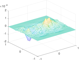
(b) $|\rho_{NN}-\rho|$

Figure 11: (a) Output of the trained network on a test sample for $K=6$, and $\alpha=10$; (b) error with respect to the reference solution.

5 Conclusion

We have developed a multiscale neural network (MNN) architecture for approximating nonlinear mappings, such as those arising from the solution of integral equations (IEs) or partial differential equations (PDEs). In order to control the number of parameters, we first rewrite the widely used hierarchical matrix into the form of a neural network, which mainly consists of three sub-networks: restriction network, kernel network, and interpolation network. The three sub-networks are all linear, and correspond to the components of a singular value decomposition. We demonstrate that such structure can be directly generalized to nonlinear problems, simply by replacing the linear kernel network by a multilayer kernel network with nonlinear activation functions. Such “nonlinear singular value decomposition operation” is performed at different spatial scales, which can be efficiently implemented by a number of locally connected (LC) networks, or convolutional neural networks (CNN) when the mapping is equivariant to translation. Using the parameterized nonlinear Schrödinger equation and the Kohn-Sham map as examples, we find that MNN can yield accurate approximation to such nonlinear mappings. When the mapping has $N$ degrees of freedom, the complexity of MNN is only $O(N\log N)$. Thus the resulting MNN can be further used to accelerate the evaluation of the mapping, especially when a large number of evaluations are needed within a certain range of parameters.

In this work, we only provide one natural architecture of multiscale neural network based on hierarchical matrices. The architecture can be altered depending on the target application. Some of the possible modifications and extensions are listed below. 1) In this work, the neural network is inspired by a hierarchical matrix with a special case of strong admissible condition. One can directly construct architectures for $\mathcal{H}$-matrices with the weak admissible condition, as well as other structures such as the fast multiple methods, $\mathcal{H}^{2}$-matrices and wavelets. 2) The input, $u$, and output, $v$, in this work are periodic. The network can be directly extended to the non-periodic case, by replacing the periodic padding in $\mathsf{LCK}$ by some other padding functions. One may also explore the mixed usage of LC networks and CNNs in different components of the architecture. 3) The matrices $A^{(\mathrm{ad})}$ and $M^{(\ell)}$ can be block-partitioned in different ways, which would result in different setups of parameters in the $\mathsf{LCK}$ layers. 4) The $\mathsf{LCR}$ and $\mathsf{LCI}$ networks in Algorithm 3 can involve nonlinear activation functions as well and can be extended to networks with more than one layer. 5) The $\mathsf{LCK}$ network in Algorithm 3 can be replaced by other architectures. In principle, for each scale, these $\mathsf{LCK}$ layers can be altered to any network, for example the sum of two parallel subnetworks, or the ResNet structure[29]. 6) It is known that $\mathcal{H}$-matrices can well approximate smooth kernels but become less efficient for highly oscillatory kernels, such as those arising from the Helmholtz operator in the high frequency regime. The range of applicability of the MNN remains to be studied both theoretically and numerically.

References

- [1] M. Abadi, P. Barham, J. Chen, Z. Chen, A. Davis, J. Dean, M. Devin, S. Ghemawat, G. Irving, M. Isard, et al. Tensorflow: A system for large-scale machine learning. In OSDI, volume 16, pages 265–283, 2016.
- [2] J. R. Anglin and W. Ketterle. Bose–Einstein condensation of atomic gases. Nature, 416(6877):211, 2002.
- [3] M. Araya-Polo, J. Jennings, A. Adler, and T. Dahlke. Deep-learning tomography. The Leading Edge, 37(1):58–66, 2018.
- [4] V. Badrinarayanan, A. Kendall, and R. Cipolla. SegNet: A deep convolutional encoder-decoder architecture for image segmentation. IEEE Transactions on Pattern Analysis and Machine Intelligence, 2017.
- [5] W. Bao and Q. Du. Computing the ground state solution of Bose–Einstein condensates by a normalized gradient flow. SIAM Journal on Scientific Computing, 25(5):1674–1697, 2004.
- [6] M. Barrault, Y. Maday, N. C. Nguyen, and A. T. Patera. An “empirical interpolation” method: application to efficient reduced-basis discretization of partial differential equations. Comptes Rendus Mathematique, 339(9):667 – 672, 2004.
- [7] C. Beck, W. E, and A. Jentzen. Machine learning approximation algorithms for high-dimensional fully nonlinear partial differential equations and second-order backward stochastic differential equations. Journal of Nonlinear Science, pages 1–57, 2017.
- [8] J. Berg and K. Nyström. A unified deep artificial neural network approach to partial differential equations in complex geometries. Neurocomputing, 317:28–41, 2018.
- [9] S. Börm, L. Grasedyck, and W. Hackbusch. Introduction to hierarchical matrices with applications. Engineering analysis with boundary elements, 27(5):405–422, 2003.
- [10] A. Brandt. Multi-level adaptive solutions to boundary-value problems. Mathematics of Computation, 31(138):333–390, 1977.
- [11] J. Bruna and S. Mallat. Invariant scattering convolution networks. IEEE Transactions on Pattern Analysis and Machine Intelligence, 35(8):1872–1886, 2013.
- [12] P. Chaudhari, A. Oberman, S. Osher, S. Soatto, and G. Carlier. Partial differential equations for training deep neural networks. In 2017 51st Asilomar Conference on Signals, Systems, and Computers, pages 1627–1631, 2017.
- [13] L. C. Chen, G. Papandreou, I. Kokkinos, K. Murphy, and A. L. Yuille. DeepLab: Semantic image segmentation with deep convolutional nets, atrous convolution, and fully connected CRFs. IEEE Transactions on Pattern Analysis and Machine Intelligence, 40(4):834–848, 2018.
- [14] F. Chollet et al. Keras. https://keras.io, 2015.
- [15] N. Cohen, O. Sharir, and A. Shashua. On the expressive power of deep learning: A tensor analysis. In Conference on Learning Theory, pages 698–728, 2016.
- [16] W. E, J. Han, and A. Jentzen. Deep learning-based numerical methods for high-dimensional parabolic partial differential equations and backward stochastic differential equations. Communications in Mathematics and Statistics, 5(4):349–380, 2017.
- [17] Y. Efendiev, J. Galvis, G. Li, and M. Presho. Generalized multiscale finite element methods. nonlinear elliptic equations. Communications in Computational Physics, 15(3):733–755, 2014.
- [18] Y. Efendiev and T. Hou. Multiscale finite element methods for porous media flows and their applications. Applied Numerical Mathematics, 57(5):577 – 596, 2007. Special Issue for the International Conference on Scientific Computing.
- [19] Y. Fan, J. Feliu-Fabà, L. Lin, L. Ying, and L. Zepeda-Núñez. A multiscale neural network based on hierarchical nested bases. Research in the Mathematical Sciences, 6(2):21, 2019.
- [20] M. Fenn and G. Steidl. FMM and -matrices: a short introduction to the basic idea. Technical Report TR-2002-008, Department for Mathematics and Computer Science, University of Mannheim, 2002.
- [21] L. Greengard and V. Rokhlin. A fast algorithm for particle simulations. Journal of computational physics, 73(2):325–348, 1987.
- [22] M. A. Grepl, Y. Maday, N. C. Nguyen, and A. T. Patera. Efficient reduced-basis treatment of nonaffine and nonlinear partial differential equations. ESAIM: Mathematical Modelling and Numerical Analysis, 41(3):575–605, 2007.
- [23] W. Hackbusch. A sparse matrix arithmetic based on -matrices. part I: Introduction to -matrices. Computing, 62(2):89–108, 1999.
- [24] W. Hackbusch, L. Grasedyck, and S. Börm. An introduction to hierarchical matrices. Math. Bohem., 127(229-241), 2002.
- [25] W. Hackbusch and B. N. Khoromskij. A sparse -matrix arithmetic: general complexity estimates. Journal of Computational and Applied Mathematics, 125(1-2):479–501, 2000.
- [26] J. Han, A. Jentzen, and W. E. Solving high-dimensional partial differential equations using deep learning. Proceedings of the National Academy of Sciences, 115(34):8505–8510, 2018.
- [27] K. He and J. Sun. Convolutional neural networks at constrained time cost. 2015 IEEE Conference on Computer Vision and Pattern Recognition (CVPR), pages 5353–5360, 2015.
- [28] K. He, X. Zhang, S. Ren, and J. Sun. Deep residual learning for image recognition. 2016 IEEE Conference on Computer Vision and Pattern Recognition (CVPR), pages 770–778, 2016.
- [29] K. He, X. Zhang, S. Ren, and J. Sun. Deep residual learning for image recognition. In Proceedings of the IEEE conference on computer vision and pattern recognition, pages 770–778, 2016.
- [30] G. Hinton, L. Deng, D. Yu, G. E. Dahl, A. r. Mohamed, N. Jaitly, A. Senior, V. Vanhoucke, P. Nguyen, T. N. Sainath, and B. Kingsbury. Deep neural networks for acoustic modeling in speech recognition: The shared views of four research groups. IEEE Signal Processing Magazine, 29(6):82–97, 2012.
- [31] P. Hohenberg and W. Kohn. Inhomogeneous electron gas. Physical review, 136(3B):B864, 1964.
- [32] K. Hornik. Approximation capabilities of multilayer feedforward networks. Neural Networks, 4(2):251–257, 1991.
- [33] Y. Khoo, J. Lu, and L. Ying. Solving parametric PDE problems with artificial neural networks. arXiv preprint arXiv:1707.03351, 2017.
- [34] V. Khrulkov, A. Novikov, and I. Oseledets. Expressive power of recurrent neural networks. arXiv:1711.00811, 2017.
- [35] N. Kishore Kumar and J. Schneider. Literature survey on low rank approximation of matrices. Linear and Multilinear Algebra, 65(11):2212–2244, 2017.
- [36] W. Kohn and L. J. Sham. Self-consistent equations including exchange and correlation effects. Physical review, 140(4A):A1133, 1965.
- [37] A. Krizhevsky, I. Sutskever, and G. E. Hinton. ImageNet classification with deep convolutional neural networks. In Proceedings of the 25th International Conference on Neural Information Processing Systems - Volume 1, NIPS’12, pages 1097–1105, USA, 2012. Curran Associates Inc.
- [38] Y. LeCun, Y. Bengio, and G. Hinton. Deep learning. Nature, 521(436), 2015.
- [39] M. K. K. Leung, H. Y. Xiong, L. J. Lee, and B. J. Frey. Deep learning of the tissue-regulated splicing code. Bioinformatics, 30(12):i121–i129, 2014.
- [40] Y. Li, X. Cheng, and J. Lu. Butterfly-Net: Optimal function representation based on convolutional neural networks. arXiv preprint arXiv:1805.07451, 2018.
- [41] L. Lin, J. Lu, and L. Ying. Fast construction of hierarchical matrix representation from matrix–vector multiplication. Journal of Computational Physics, 230(10):4071–4087, 2011.
- [42] G. Litjens, T. Kooi, B. E. Bejnordi, A. A. A. Setio, F. Ciompi, M. Ghafoorian, J. A. W. M. van der Laak, B. van Ginneken, and C. I. Sánchez. A survey on deep learning in medical image analysis. Medical Image Analysis, 42:60–88, 2017.
- [43] R. M. Forward-backward stochastic neural networks: Deep learning of high-dimensional partial differential equations. arXiv:1804.07010, 2018.
- [44] J. Ma, R. P. Sheridan, A. Liaw, G. E. Dahl, and V. Svetnik. Deep neural nets as a method for quantitative structure-activity relationships. Journal of Chemical Information and Modeling, 55(2):263–274, 2015.
- [45] Y. Maday, O. Mula, and G. Turinici. Convergence analysis of the generalized empirical interpolation method. SIAM Journal on Numerical Analysis, 54(3):1713–1731, 2016.
- [46] S. Mallat. A wavelet tour of signal processing: the sparse way. Academic press, Boston, third edition, 2008.
- [47] M. Mathieu, C. Couprie, and Y. LeCun. Deep multi-scale video prediction beyond mean square error. arXiv:1511.05440, abs/1712.04741, 2016.
- [48] H. Mhaskar, Q. Liao, and T. Poggio. Learning functions: When is deep better than shallow. arXiv preprint arXiv:1603.00988, 2016.
- [49] P. Paschalis, N. D. Giokaris, A. Karabarbounis, G. Loudos, D. Maintas, C. Papanicolas, V. Spanoudaki, C. Tsoumpas, and E. Stiliaris. Tomographic image reconstruction using artificial neural networks. Nuclear Instruments and Methods in Physics Research Section A: Accelerators, Spectrometers, Detectors and Associated Equipment, 527(1):211 – 215, 2004. Proceedings of the 2nd International Conference on Imaging Technologies in Biomedical Sciences.
- [50] D. M. Pelt and J. A. Sethian. A mixed-scale dense convolutional neural network for image analysis. Proceedings of the National Academy of Sciences, 115(2):254–259, 2018.
- [51] L. Pitaevskii. Vortex lines in an imperfect Bose gas. Sov. Phys. JETP, 13(2):451–454, 1961.
- [52] M. Raissi and G. E. Karniadakis. Hidden physics models: Machine learning of nonlinear partial differential equations. Journal of Computational Physics, 357:125 – 141, 2018.
- [53] O. Ronneberger, P. Fischer, and T. Brox. U-Net: Convolutional networks for biomedical image segmentation. In N. Navab, J. Hornegger, W. M. Wells, and A. F. Frangi, editors, Medical Image Computing and Computer-Assisted Intervention – MICCAI 2015, pages 234–241, Cham, 2015. Springer International Publishing.
- [54] K. Rudd, G. D. Muro, and S. Ferrari. A constrained backpropagation approach for the adaptive solution of partial differential equations. IEEE Transactions on Neural Networks and Learning Systems, 25(3):571–584, 2014.
- [55] J. Schmidhuber. Deep learning in neural networks: An overview. Neural Networks, 61:85–117, 2015.
- [56] J. Sirignano and K. Spiliopoulos. DGM: A deep learning algorithm for solving partial differential equations. Journal of Computational Physics, 375:1339–1364, 2018.
- [57] I. Sutskever, O. Vinyals, and Q. V. Le. Sequence to sequence learning with neural networks. In Z. Ghahramani, M. Welling, C. Cortes, N. D. Lawrence, and K. Q. Weinberger, editors, Advances in Neural Information Processing Systems 27, pages 3104–3112. Curran Associates, Inc., 2014.
- [58] D. Timothy. Incorporating Nesterov momentum into Adam. International Conference on Learning Representations, 2015.
- [59] L. Trefethen. Spectral Methods in MATLAB. Society for Industrial and Applied Mathematics, 2000.
- [60] D. Ulyanov, A. Vedaldi, and V. Lempitsky. Deep image prior. In Proceedings of the IEEE Conference on Computer Vision and Pattern Recognition, pages 9446–9454, 2018.
- [61] Y. Wang, C. W. Siu, E. T. Chung, Y. Efendiev, and M. Wang. Deep multiscale model learning. arXiv preprint arXiv:1806.04830, 2018.
- [62] C. Zhang, S. Bengio, M. Hardt, B. Recht, and O. Vinyals. Understanding deep learning requires rethinking generalization. arXiv:1611.03530, 2016.
- [63] K. Zhang, W. Zuo, Y. Chen, D. Meng, and L. Zhang. Beyond a Gaussian denoiser: Residual learning of deep CNN for image denoising. IEEE Transactions on Image Processing, 26(7):3142–3155, 2017.
- [64] L. Zhang, J. Han, H. Wang, R. Car, and W. E. DeePCG: constructing coarse-grained models via deep neural networks. arXiv preprint arXiv:1802.08549, 2018.
- [65] L. Zhang, H. Wang, and W. E. Adaptive coupling of a deep neural network potential to a classical force field. arXiv preprint arXiv:1806.01020, 2018.