Renewal-scaled solutions of the Kolmogorov forward equation for residual times
Abstract
Let be a renewal process for independent holding times ,where are identically distributed with density . If the associated residual time has a density , its Kolmogorov forward equation is given by
with an initial holding time density . We derive a measure-valued solution formula for the density of residuals times after an expected number of renewals occur. Solutions under this time scale are then shown to evolve continuously in the space of measures with the weak topology under mild conditions.
MSC classification: 60K05
Keywords: Kolmogorov forward equation, residual time, renewal theory
1 Introduction
Let be a sequence of iid random variables in called holding times, each having a density . Also define a random initial holding time , independent from , but possibly distinct in law. The renewal process associated with counts the number of renewals up to time , and is given by
| (1.1) |
Related to the renewal process is the residual time (also known as the forward recurrence time), defined as
| (1.2) |
At time , is the time remaining until the next renewal. Residual times are fundamental in renewal theory and queueing theory (see Ch. 9 of Cox [2] for a detailed introduction), and may be viewed as an extension of homogeneous Poisson processes, in which holding times, and consequently residual times, are exponentially distributed [9].
If has a differentiable density in time and space , then the Kolmogorov forward equation for residual times is given by
| (1.3) |
This equation has the explicit solution (see Pg. 63 of [1]) of
| (1.4) |
Here, is the renewal density
| (1.5) |
where denotes -fold self-convolution (with the convention and ). An important fact (see Sect. 9.12 in [10]) is that
| (1.6) |
In Section 2.1 we derive (1.3) through asymptotic expansions, and in Section 2.2, we derive (1.4) through Laplace transforms, a method similar to [4].
The main novelty of this paper is a change of variables for (1.3) based on expected renewals, presented in Section 3. Specifically, we introduce the new time scale Using the time scale is a natural option for several scenarios in queuing theory. For an example, consider a factory lit by a large collection of light bulbs, running simultaneously. When a bulb breaks, it is immediately replaced by a new light bulb with a random run length distributed with respect to . If the initial distribution of run lengths at time zero for the bulbs is approximately , then estimates remaining run lengths at time . What, then, is the distribution of remaining run lengths after light bulbs have been replaced? The answer to this question is provided through the renewal-scaled solution formula (3.6). Given the expansive history of renewal theory, the author expected to find (3.6) in the literature, but was unable to do so after a thorough search.
Both the change of time scale and method for renewal-scaled solutions are motivated by the work of Menon, Niethammer, and Pego in [8], who investigated a wide range of clustering events generalizing the 1D Allen-Cahn equation in mathematical physics. The measure-valued space of clusters was shown to be continuous in time in the space of probability measures through using an intrinsic time scale based on the number of clusters in the system. In our case, we define measure-valued solutions of (1.3) in the time scale which evolve continuously in under a wide range of holding times. We conclude with an example in Section 3.3, which illustrates with how renewal-scaled solutions continuously evolve under initial holding times with point masses.
2 Strong solutions
2.1 Derivation of forward equation
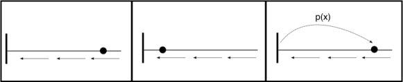
In this section will use an equivalent reformulation for from the perspective of a random dynamical system. This is done by considering a particle at time randomly placed on , with its initial position given by the first holding time . The particle drifts toward the origin at unit speed until it reaches the origin at time . At this time, it is immediately reassigned to , distributed with respect to . The particle proceeds as before, moving toward the origin and being reassigned upon its arrival, with and iid (see Figure 2.1). It is clear that the position of the particle at time corresponds with the residual time under holding times
To derive (1.3), we will compute asymptotics for probabilities that a particle is in a small interval. Assume for now that is continuous, and is differentiable in both and . Then an asymptotic expansion for the probability that a particle is in at time is
| (2.1) |
Next, we consider the probability that the particle at initial time is contained in at time . This can occur in two ways. The simplest case is when the particle is initially in . Denote this event , whose probability has the expansion
| (2.2) |
The second case is when a particle begins in , reaches the origin, and is reassigned before drifting into at time . Denote this event . We may partition this event according to the particle’s initial position , and how many times the particle jumps. Then
| (2.3) |
Since , we compare terms in (2.1), (2.2), and (2.3) to arrive at (1.3).
2.2 Classical solutions
In this section, we will derive the solution formula (1.4) for initial conditions in the space
| (2.4) |
Definition 1.
Let . A function with which solves is a strong solution.
Our first step in finding an explicit strong solution formula is integrating (1.3) along characteristics , which gives us the integral form of (1.3)
| (2.5) |
By comparing (1.4) and (2.5), we see that finding an explicit solution formula is equivalent to showing . This in fact follows immediately by simply setting in (2.5), from which we obtain the well-known renewal equation whose solution is . However, we derive here the explicit formula for , as some of the intermediate formulas produced will be of use in later sections.
Toward this end, we apply the Laplace transform
| (2.6) |
to both sides of (1.3) to yield
| (2.7) |
This may easily be solved for , with
| (2.8) |
This solution is similar to (1.4), but now we can use Laplace inversion to extract a formula for . Since we are taking the Laplace transform of a probability density, for . Thus as . We then can obtain, from the limit of (2.8),
| (2.9) |
We now have a formula for based on the initial data. Notice that the left hand side is a Laplace transform in the spatial variable, whereas the right hand side is a Laplace transform of in the time variable.
To perform Laplace inversion on (2.9), observe that is a probability density, so that for . Thus, we can express the left hand side of (2.9) as the geometric series
| (2.10) |
From the convolution formula, our renewal density has an explicit expression
| (2.11) |
which is equivalent to . Since is locally integrable (Th. 3.18 of [6]), (1.4) is well-defined, is differentiable in both spatial and time variables, and for fixed , as . Finally, we may show that is a probability density for each integrating (1.3) with respect to the variable. We summarize our findings in
3 Rescaling by expected renewals
In preparation for defining measure-valued solutions in the next section, we’ll first reformulate (1.3) in terms of probability measures . In one dimension a probability measure may may be identified with its cumulative distribution function . In the future, when no confusion arises, we will often write The Laplace transform of a measure is then defined as
| (3.1) |
If a measure admits a density , then .
For , (2.7) may be rewritten in terms of measures as
| (3.2) |
where and . Since and are strictly positive and continuous, so is , and thus is strictly increasing and differentiable, with . We may now transform (3.2) as
From the chain rule, we now convert to the time scale, with
| (3.3) |
where we now define . This in turn gives us the solution formula
| (3.4) |
Since as , the limit of (3.4) is then
| (3.5) |
and consequently takes the simple form
| (3.6) |
3.1 Extension to measure valued solutions
The solution formula (3.6) has only been defined for the strict class of functions , but its form suggests that we may directly extend solutions for measures . To do so, however, we require a proper extension for , since the trace assumes solutions have a density. Nonetheless, we can use formula (2.11) to define
| (3.7) |
where convolution of the two measures and is defined as
| (3.8) |
For a sequence of measures , and converging weakly in , then by Prokhorov’s theorem, and are tight, and weakly. We may use this to show that is nondecreasing for arbitrary measures by regularization.
Even with a proper notion of , still more is required to make (3.6) well-defined for measures. This is because may be constant on an interval, or have jumps, both of which prohibit an inverse with a domain defined on all of . To address this, we use a generalized notion of inverse for nondecreasing functions. For a nondecreasing function , define the generalized inverse by
| (3.9) |
When is strictly increasing and continuous, the usual inverse and generalized inverse coincide. For a generic distribution , we define
| (3.10) |
3.2 Properties of renewal-scaled solutions
Here we will demonstrate that the extension of the solution for strong solutions to include measure-valued initial data and holding times is natural in the sense that measure-valued renewal-scaled solutions are weak limits of strong solutions in the time scale. We also show that our rescaling has the effect of smoothing point masses approaching the origin, as weak solutions evolve continuously so long as is strictly increasing.
Theorem 4.
Let be nondefective (meaning ). The following hold:
(1) Let be a sequence of strong solutions with initial conditions and holding time densities , and let be the corresponding renewal-scaled solutions. Suppose is renewal-scaled solution for initial data and holding time measure . Then if and weakly, then weakly at all points of continuity of .
(2) For any , is a probability measure for all .
(3) If is strictly increasing, then for , the map is continuous in under the weak topology.
Remark 5.
Since is dense in , for any we can always find with and weakly. Thus, for points of continuity of , we can define renewal-scaled solutions through weak limits of strong solutions.
Remark 6.
The possible nonconvergence at jump points of is essentially due to the multiple ways that one can define a generalized inverse for increasing functions. In our definition, inverses of cadlag functions remain cadlag, whereas using the traditional definition of a quantile from statistics, for instance, would instead give caglad functions.
Remark 7.
We note that for statement (3), there are a variety of sufficient and which produce strictly increasing for . One such sufficient condition, for instance, is if is strictly increasing on an interval about the origin. The point here is that jumps in the solution only occur when is constant in an interval. As we will see in Section 3.3, point masses arriving at the origin (corresponding to jumps in ) are continuously redistributed in the time scale.
Proof.
(1) Renewal-scaled solutions for satisfy
| (3.11) |
To show weak convergence, it is enough to show . We first wish to show that weakly. This follows from the continuity theorem [3, XIII.1], which states that weak convergence of locally finite measures is equivalent to pointwise convergence of their Laplace transforms. From (2.9),
| (3.12) |
Weak equivalence of measures implies that cumulative functions converge to at all continuity points of . Now, for all points of continuity of , [8, Lemma 3.1]. As the generalized inverse is a nondecreasing function, its discontinuity set is countable, and thus almost everywhere.
What remains is to show convergence of the integrals
| (3.13) |
Here, we will use the dominated convergence theorem. This requires bounding the integrand , which we obtain from several steps:
(i) Observe that there exist and a positive integer such that is a point of continuity for , and for . Define truncated holding times which are restricted to , with cumulative functions
| (3.14) |
Denote and as random variables distributed with respect to and , respectively. Then clearly weakly, and since , it follows that
(ii) Since is supported on a finite interval, it has a finite first and second moment. Thus allows us to apply Lorden’s estimate [7] to obtain
| (3.15) |
Note that we have added 1 to Lorden’s original estimate to account for a possibly distinct initial holding time.
(iii) Since are all supported in , it follows that weak convergence to implies the convergence of moments. From this and (3.15) it is straightforward to show that there exist such that for all positive ,
| (3.16) |
| (3.17) |
Thus, integrands in the left hand side of (3.13) are dominated by an exponentially decaying function, which proves (3.13) and thus part (1).
Part (2) follows immediately from the weak convergence shown in part (1), since are all probability measures.
For part (3), note that if is strictly increasing, then is continuous. From (3.6), it is clear that is continuous in , which in turn implies that evolves continuously under the weak topology in the space of measures. ∎
3.3 An example of renewal-scaled solutions with point mass initial conditions
To illustrate how renewal-scaled solutions behave under jumps in initial data, we conclude with an example with monodisperse initial conditions. Specifically, let the initial measure data satisfy and . Then , and using (2.9),
| (3.18) |
For , Laplace inversion then gives
| (3.19) |
which has a generalized inverse of
| (3.20) |
Substitution of these variables into (3.6), for , yields
Taking inverse Laplace transforms then gives us the solution for . By a similar calculation, we can show that for .
In the time scale, initial conditions with a support not containing the origin will immediately jump through translation. For our example, the point mass jumps to the origin, and is then continuously reassigned to according to at a constant rate of one. After the reassignment of the entire point mass, the solution, now a density, is stationary, since is a solution to (1.3) with (one can see, in fact, that this is a manifestation of the memoryless property of exponential distributions).
4 Acknowledgements
The author is indebted to Robert Pego and Govind Menon for multiple conversions regarding the preparation of his thesis [5], a chapter of which is the basis of this paper.
5 Conflicts of Interest
The author declares no conflict of interest.
References
- [1] D. R. Cox, Renewal theory, vol. 1, Methuen London, 1967.
- [2] , The theory of stochastic processes, Routledge, 2017.
- [3] W. Feller, An introduction to probability theory and its applications, vol. 2, John Wiley & Sons, 2008.
- [4] J. W. Kim and G. C. Shim, A Markovian approach to the forward recurrence time in the renewal process, JKSS (Journal of the Korean Statistical Society), 33 (2004), pp. 299–302.
- [5] J. Klobusicky, Kinetic limits of piecewise deterministic Markov processes and grain boundary coarsening, PhD thesis, Brown University, Providence, RI, 2014.
- [6] M. Liao, Applied stochastic processes, CRC Press, 2013.
- [7] G. Lorden, On excess over the boundary, The Annals of Mathematical Statistics, (1970), pp. 520–527.
- [8] G. Menon, B. Niethammer, and R. Pego, Dynamics and self-similarity in min-driven clustering, Transactions of the American Mathematical Society, 362 (2010), pp. 6591–6618.
- [9] S. I. Resnick, Adventures in stochastic processes, Springer Science & Business Media, 2013.
- [10] W. J. Stewart, Probability, Markov chains, queues, and simulation: the mathematical basis of performance modeling, Princeton University Press, 2009.