Software paper for submission to the Journal of Open Research Software

To complete this template, please replace the blue text with your own. The paper has three main sections: (1) Overview; (2) Availability; (3) Reuse potential.

Please submit the completed paper to: editor.jors@ubiquitypress.com

 

(1) Overview

Title

FluidFFT: common API (C++ and Python) for Fast Fourier Transform HPC libraries

Paper Authors

1. MOHANAN Ashwin Vishnu^a
2. BONAMY Cyrille^b
3. AUGIER Pierre^b

^a Linné Flow Centre, Department of Mechanics, KTH, 10044 Stockholm, Sweden. ^b Univ. Grenoble Alpes, CNRS, Grenoble INP, LEGI, 38000 Grenoble, France.

Paper Author Roles and Affiliations

1. Ph.D. student, Linné Flow Centre, KTH Royal Institute of Technology, Sweden;
2. Research Engineer, LEGI, Université Grenoble Alpes, CNRS, France;
3. Researcher, LEGI, Université Grenoble Alpes, CNRS, France

Abstract

The Python package fft provides a common Python API for performing Fast Fourier Transforms (FFT) in sequential, in parallel and on GPU with different FFT libraries (FFTW, P3DFFT, PFFT, cuFFT). fft is a comprehensive FFT framework which allows Python users to easily and efficiently perform FFT and the associated tasks, such as as computing linear operators and energy spectra. We describe the architecture of the package composed of C++ and Cython FFT classes, Python “operator” classes and Pythran functions. The package supplies utilities to easily test itself and benchmark the different FFT solutions for a particular case and on a particular machine. We present a performance scaling analysis on three different computing clusters and a microbenchmark showing that fft is an interesting solution to write efficient Python applications using FFT.

Keywords

Free and open-source library; Python; Fast Fourier Transform; Distributed; MPI; GPU; High performance computing

Introduction

Fast Fourier Transform (FFT) is a class of algorithms used to calculate the discrete Fourier transform, which traces back its origin to the groundbreaking work by Cooley & Tukey (1965). Ever since then, FFT as a computational tool has been applied in multiple facets of science and technology, including digital signal processing, image compression, spectroscopy, numerical simulations and scientific computing in general. There are many good libraries to perform FFT, in particular the de-facto standard FFTW (Frigo & Johnson, 2005). A challenge is to efficiently scale FFT on clusters with the memory distributed over a large number of cores using Message Passing Interface (MPI). This is imperative to solve big problems faster and when the arrays do not fit in the memory of single computational node. A problem is that for one-dimensional FFT, all the data have to be located in the memory of the process that perform the FFT, so a lot of communications between processes are needed for 2D and 3D FFT.

There are two strategies to distribute an array in the memory, the 1D (or slab) decomposition and the 2D (or pencil) decomposition. The 1D decomposition is more efficient when only few processes are used but suffers from an important limitation in terms of number of MPI processes that can be used. Utilizing 2D decomposition overcomes this limitation.

Some of the well-known libraries are written in C, C++ and Fortran. The classical FFTW library supports MPI using 1D decomposition and hybrid parallelism using MPI and OpenMP. Other libraries, now implement the 2D decomposition: PFFT (Pippig, 2013), P3DFFT (Pekurovsky, 2012), 2decomp&FFT and so on. These libraries rely on MPI for the communications between processes, are optimized for supercomputers and scales well to hundreds of thousands of cores. However, since there is no common API, it is not simple to write applications that are able to use these libraries and to compare their performances. As a result, developers are met with a hard decision, which is to choose a library before the code is implemented.

Apart from CPU-based parallelism, General Purpose computing on Graphical Processing Units (GPGPU) is also gaining traction in scientific computing. Scalable libraries written for GPGPU such as OpenCL and CUDA have emerged, with their own FFT implementations, namely clFFT and cuFFT respectively.

Python can easily link these libraries through compiled extensions. For a Python developer, the following packages leverage this approach to perform FFT:

sequential FFT, using: numpy.fft and scipy.fftpack which are essentially C and Fortran extensions for FFTPACK library. pyFFTW which wraps FFTW library and provides interfaces similar to the numpy.fft and scipy.fftpack implementations. mkl_fft, which wraps Intel’s MKL library and exposes python interfaces to act as drop-in replacements for numpy.fft and scipy.fftpack. FFT with MPI, using: mpiFFT4py and mpi4py-fft built on top of pyFFTW and numpy.fft. pfft-python which provides extensions for PFFT library. FFT with GPGPU, using: Reikna, a pure python package which depends on PyCUDA and PyOpenCL pytorch-fft: provides C extensions for cuFFT, meant to work with PyTorch, a tensor library similar to NumPy.

Although these Python packages are under active development, they suffer from certain drawbacks:

• No effort so far to consolidate all possible FFT libraries, both sequential, MPI and GPGPU based under a single package with similar syntax.

• Quite complicated even for the simplest use case scenarios. To understand how to use them, a novice user has to, at least, read the FFTW documentation.

• No benchmarks between libraries and between the Python solutions and solutions based only on a compiled language (as C, C++ or Fortran).

• Provides just the FFT and inverse FFT functions, no associated mathematical operators.

The Python package fft fills this gap by providing C++ classes and their Python wrapper classes for performing simple and common tasks with different FFT libraries. It has been written to make things easy while being as efficient as possible. It provides:

• tests,

• documentation and tutorials,

• benchmarks,

• operators for simple tasks (for example, compute the energy or the gradient of a field).

In the present article, we shall start by describing the implementation of fft including its design aspects and the code organization. Thereafter, we shall compare the performance of different classes in fft in three computing clusters, and also describe, using microbenchmarks, how a Python function can be optimized to be as fast as a Fortran implementation. Finally, we show how we test and maintain the quality of the code base through continuous integration and mention some possible applications of fft.

Implementation and architecture

The two major design goals of fft are:

• to support multiple FFT libraries under the same umbrella and expose the interface for both C++ and Python code development.

• to keep the design of the interfaces as human-centric and easy to use as possible, without sacrificing performance.

Both C++ and Python APIs provided by fft currently support linking with FFTW (with and without MPI and OpenMP support enabled), MKL, PFFT, P3DFFT, cuFFT libraries. The classes in fft offers API for performing double-precision computation with real-to-complex FFT, complex-to-real inverse FFT, and additional helper functions.

C++ API

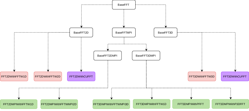
Figure 1: Class hierarchy demonstrating object-oriented approach. The sequential classes are shown in red, the CUDA-based classes in magenta and the MPI-based classes in green. The arrows represent inheritance from parent to child class.

The C++ API is implemented as a hierarchy of classes as shown in Fig. 1. The naming convention used for the classes (¡Type of FFT¿With¡Name of Library¿) is a cue for how these are functioning internally. By utilizing inheritance, the classes share the same function names and syntax defined in the base classes, shown in white boxes in Fig. 1. Some examples of such functions are:

• alloc_array_X: Allocates array to store a physical array with real datatype for the current process.

• alloc_array_K: Allocates array to store a spectral array with complex datatype for the current process.

• init_array_X_random: Allocates and initializes a physical array with random values.

• test: Run tests for a class by comparing mean and mean energy values in an array before and after a set of fft and ifft calls.

• bench: Benchmark the fft and ifft methods for certain number of iterations.

Remaining methods which are specific to a library are defined in the corresponding child classes, depicted in coloured boxes in Fig. 1, for example:

• are_parameters_bad: Verifies whether the global array shape can be decomposed with the number of MPI processes available or not. If the parameters are compatible, the method returns false. This method is called prior to initializing the class.

• fft and ifft: Forward and inverse FFT methods.

Let us illustrate with a trivial example, wherein we initialize the FFT with a random physical array, and perform a set of fft and ifft operations.

⬇

#include <iostream>

using namespace std;

\par#include <fft3dmpi_with_fftwmpi3d.h>

// #include <fft3dmpi_with_p3dfft.h>

\parint main(int argc, char **argv) {

int N0 = N1 = N2 = 32;

// MPI-related

int nb_procs = 4;

MPI_Init(&argc, &argv);

MPI_Comm_size(MPI_COMM_WORLD, &(nb_procs));

\parmyreal* array_X;

mycomplex* array_K;

\parFFT3DMPIWithFFTWMPI3D o(N0, N1, N2);

// FFT3DMPIWithP3DFFT o(N0, N1, N2);

\paro.init_array_X_random(array_X);

o.alloc_array_K(array_K);

o.fft(array_X, array_K);

o.ifft(array_K, array_X);

MPI_Finalize();

return 0;

}

As suggested through comments above, in order to switch the FFT library, the user only needs to change the header file and the class name. An added advantage is that, the user does not need to bother about the domain decomposition while declaring and allocating the arrays. A few more helper functions are available with the FFT classes, such as functions to compute the mean value and energies in the array. These are demonstrated with examples in the documentation. Detailed information regarding the C++ classes and its member functions are also included in the online documentation.

Python API

Similar to other packages in the FluidDyn project, fft also uses an object-oriented approach, providing FFT classes. This is in contrast with the approach adopted by numpy.fft and scipy.fftpack which provides functions instead, with which the user has to figure out the procedure to design the input values and to use the return values, from the documentation. In fft, the Python API wraps all the functionalities of its C++ counterpart and offers a more richer experience through an accompanying operator class.

As a short example, let us try to calculate the gradient of a plane sine-wave using spectral methods, mathematically described as follows:

$$u(x,y) =\sin(x+y) \forall x,y\in\left[0,L\right]$$

$$\hat{u}(k_{x},k_{y}) =\frac{1}{L^{2}}\int_{0}^{L}\int_{0}^{L}u(x,y)\exp(ik_{x}x+ik_{y}y)dxdy$$

$$\nabla u(x,y) =\sum_{k_{x}}\sum_{k_{y}}i\mathbf{k}\hat{u}(k_{x},k_{y})\exp(-ik_{x}x-ik_{y}y)$$

where $k_{x}$, $k_{y}$ represent the wavenumber corresponding to x- and y-directions, and $\mathbf{k}$ is the wavenumber vector.

The equivalent pseudo-spectral implementation in fft is as follows:

⬇

from fluidfft.fft2d.operators import OperatorsPseudoSpectral2D, pi

from numpy import sin

\parnx = ny = 100

lx = ly = 2 * pi

\paroper = OperatorsPseudoSpectral2D(nx, ny, lx, ly, fft=”fft2d.with_fftw2d”)

\paru = sin(oper.XX + oper.YY)

u_fft = oper.fft(u)

px_u_fft, py_u_fft = oper.gradfft_from_fft(u_fft)

px_u = oper.ifft(px_u_fft)

py_u = oper.ifft(py_u_fft)

grad_u = (px_u, py_u)

A parallelized version of the code above will work out of the box, simply by replacing the FFT class with an MPI-based FFT class, for instance fft2d.with_fftwmpi2d. One can also let fft automatically choose an appropriate FFT class by instantiating the operator class with fft=None or fft=”default”. Even if one finds the methods in the operator class to be lacking, one can inherit the class and easily create a new method, for instance using the wavenumber arrays, oper.KX and oper.KY. Arguably, a similar implementation with other available packages would require the know-how on how FFT arrays are allocated in the memory, normalized, decomposed in parallel and so on. Moreover, the FFT and the operator classes contain objects describing the shapes of the real and complex arrays and how the data is shared between processes. A more detailed introduction on how to use fft and available functions can be found in the tutorials.

Thus, we have demonstrated how, by using fft, a developer can easily switch between FFT libraries. Let us now turn our attention to how the code is organized. We shall also describe how the source code is built, and linked with the supported libraries.

Code organization

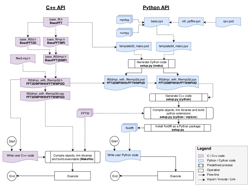
Figure 2: Flowchart illustrating how the C++ and Python API are built and used for one particular class, viz. FFT2DMPIWithFFTWMPI2D. The dotted arrows in C++ part stand for include statements, demonstrating the class hierarchy and in the Python part indicate how different codes are imported. On the bottom, a smaller flowchart demonstrates how to use the API by writing user code.

The internal architecture of fft can be visualized as layers. Through Fig. 2, we can see how these layers are linked together forming the API for C++ and Python development. For simplicity, only one FFT class is depicted in the figure, namely FFT2DMPIWithFFTWMPI2D, which wraps FFTW’s parallelized 2D FFT implementation. The C++ API is accessed by importing the appropriate header file and building the user code with a Makefile, an example of which is available in the documentation.

The Python API is built automatically when fft is installed. It first generates the Cython source code as a pair of .pyx and .pxd files containing a class wrapping its C++ counterpart. The Cython files are produced from template files (specialized for the 2D and 3D cases) using the template library . Thereafter, Cython (Behnel et al., 2011) generates C++ code with necessary Python bindings, which are then built in the form of extensions or dynamic libraries importable in Python code. All the built extensions are then installed as a Python package fft.

A helper function fluidfft.import_fft_class is provided with the package to simply import the FFT class. However, it is more convenient and recommended to use an operator class, as described in the example for Python API. Although the operator classes can function as pure Python code, some of its critical methods can be compiled, if Pythran (Guelton, 2018) is available during installation of fft. We will show towards the end of this section that by using Pythran, we reach the performance of the equivalent Fortran code.

To summarize, fft consists of the following layers:

• One C++ class per method derived from a hierarchy of C++ classes as shown in Fig. 1.

• Cython wrappers of the C++ classes with their unit test cases.

• Python operators classes (2D and 3D) to write code independently of the library used for the computation of the FFT and with some mathematical helper methods. These classes are accompanied by unit test cases.

• Pythran functions to speedup critical methods in the Python operators classes.

Command-line utilities (fluidfft-bench and fluidfft-bench-analysis) are also provided with the fft installation to run benchmarks and plot the results. In the next subsection, we shall look at some results by making use of these utilities on three computing clusters.

Performance

Scalability tests using fluidfft-bench

Scalability of fft is measured in the form of strong scaling speedup, defined in the present context as:

$$S_{\alpha}(n_{p})=\frac{[\mathrm{Time\ elapsed\ for\ }N\mathrm{\ iterations\ with\ }n_{p,\min}\mathrm{\ processes}]_{\mathrm{fastest}}\times n_{p,\min}}{[\mathrm{Time\ elapsed\ for\ }N\mathrm{\ iterations\ with\ }n_{p}\mathrm{\ processes}]_{\alpha}}$$

where $n_{p,\min}$ is the minimum number of processes employed for a specific array size and hardware. The subscripts, $\alpha$ denotes the FFT class used and “fastest” corresponds to the fastest result among various FFT classes.

To compute strong scaling the utility fluidfft-bench is launched as scheduled jobs on HPC clusters, ensuring no interference from background processes. No hyperthreading was used. We have used $N=20$ iterations for each run, with which we obtain sufficiently repeatable results. For a particular choice of array size, every FFT class available are benchmarked for the two tasks, forward and inverse FFT. Three different function variants are compared (see the legend in subsequent figures):

• fft_cpp, ifft_cpp (continuous lines): benchmark of the C++ function from the C++ code. An array is passed as an argument to store the result. No memory allocation is performed inside these functions.

• fft_as_arg, ifft_as_arg (dashed lines): benchmark of a Python method from Python. Similar to the C++ code, the second argument of this method is an array to contain the result of the transform, so no memory allocation is needed.

• fft_return, ifft_return (dotted lines): benchmark of a Python method from Python. No array is provided to the function to contain the result, and therefore a numpy array is created and then returned by the function.

On big HPC clusters, we have only focussed on 3D array transforms as benchmark problems, since these are notoriously expensive to compute and require massive parallelization. The physical arrays used in all four 3D MPI based FFT classes are identical in structure. However, there are subtle differences, in terms of how the domain decomposition and the allocation of the transformed array in the memory are handled.

Hereafter, for the sake of brevity, the FFT classes will be named in terms of the associated library (For example, the class FFT3DMPIWithFFTW1D is named fftw1d). Let us go through the results plotted using fluidfft-bench-analysis.

Benchmarks on Occigen

Occigen is a GENCI-CINES HPC cluster which uses Intel Xeon CPU E5–2690 v3 (2.6 GHz) processors with 24 cores per node. The installation was performed using Intel C++ 17.2 compiler, Python 3.6.5, and OpenMPI 2.0.2.

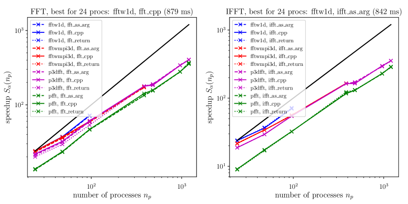
Figure 3: Speedup computed from the median of the elapsed times for 3D fft (384$\times$1152$\times$1152, left: fft and right: ifft) on Occigen.

Fig. 3 demonstrates the strong scaling performance of a cuboid array sized $384\times 1152\times 1152$. This case is particularly interesting since for FFT classes implementing 1D domain decomposition (fftw1d and fftwmpi3d), the processes are spread on the first index for the physical input array. This restriction is as a result of some FFTW library internals and design choices adopted in fft. This limits fftw1d to 192 cores and fftwmpi3d to 384 cores. The latter can utilize more cores since it is capable of working with empty arrays, while sharing some of the computational load. The fastest methods for relatively low and high number of processes are fftw1d and p3dfft respectively for the present case.

The benchmark is not sufficiently accurate to measure the cost of calling the functions from Python (difference between continuous and dashed lines, i.e. between pure C++ and the as_arg Python method) and even the creation of the numpy array (difference between the dashed and the dotted line, i.e. between the as_arg and the return Python methods).

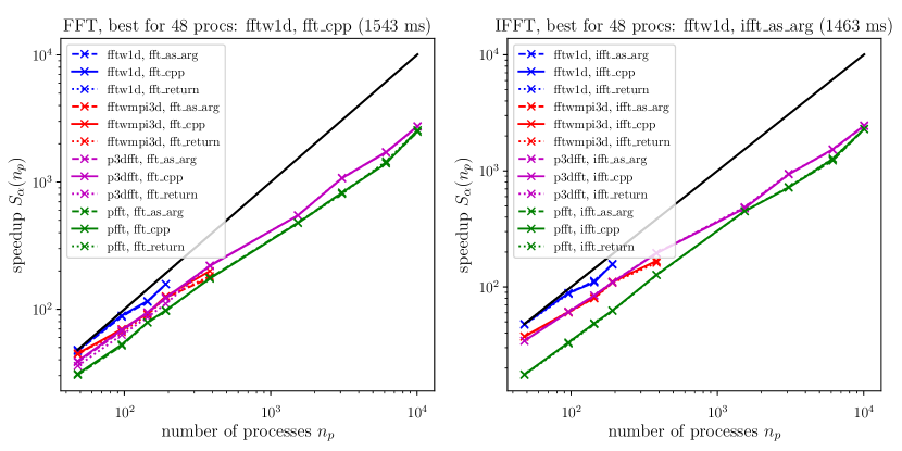
Figure 4: Speedup computed from the median of the elapsed times for 3D fft (1152$\times$1152$\times$1152, left: fft and right: ifft) on Occigen.

Fig. 4 demonstrates the strong scaling performance of a cubical array sized $1152\times 1152\times 1152$. For this resolution as well, fftw1d is the fastest method when using only few cores and it can not be used for more that 192 cores. The faster library when using more cores is also p3dfft. This also shows that fft can effectively scale for over 10,000 cores with a significant increase in speedup.

Benchmarks on Beskow

Beskow is a Cray machine maintained by SNIC at PDC, Stockholm. It runs on Intel(R) Xeon(R) CPU E5-2695 v4 (2.1 GHz) processors with 36 cores per node. The installation was done using Intel C++ 18 compiler, Python 3.6.5 and CRAY-MPICH 7.0.4.

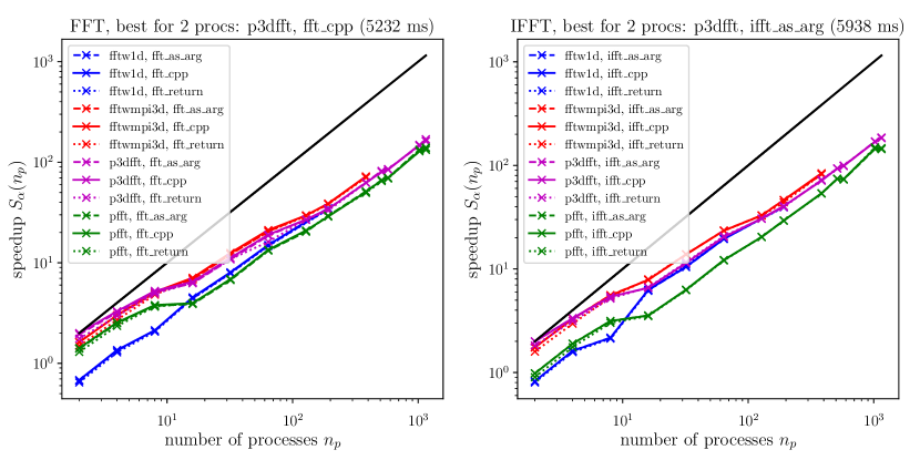
Figure 5: Speedup computed from the median of the elapsed times for 3D fft (384$\times$1152$\times$1152, left: fft and right: ifft) on Beskow.

In Fig. 5, the strong scaling results of the cuboid array can be observed. In this set of results we have also included intra-node scaling, wherein there is no latency introduced due to typically slower node-to-node communication. The fastest library for very low (below 16) and very high (above 384) number of processes in this configuration is p3dfft. For moderately high number of processes (16 and above) the fastest library is fftwmpi3d. Here too, we notice that fftw1d is limited to 192 cores and fftwmpi3d to 384 cores, for reasons mentioned earlier.

A striking difference when compared with Fig. 3 is that fftw1d is not the fastest of the four classes in this machine. One can only speculate that this could be a consequence of the differences in MPI library and hardware which has been employed. This also emphasises the need to perform benchmarks when using an entirely new configuration.

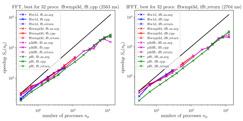
Figure 6: Speedup computed from the median of the elapsed times for 3D fft (1152$\times$1152$\times$1152, left: fft and right: ifft) on Beskow.

The strong scaling results of the cubical array on Beskow are displayed on Fig. 6, wherein we restrict to inter-node computation. We observe that the fastest method for low number of processes is again, fftwmpi3d. When high number of processes (above 1000) are utilized, initially p3dfft is the faster methods as before, but with 3000 and above processes, pfft is comparable in speed and sometimes faster.

Benchmarks on a LEGI cluster

Let us also analyse how fft scales on a computing cluster maintained at an institutional level, named Cluster8 at LEGI, Grenoble. This cluster functions using Intel Xeon CPU E5-2650 v3 (2.3 GHz) with 20 cores per node and fft was installed using a toolchain which comprises of gcc 4.9.2, Python 3.6.4 and OpenMPI 1.6.5 as key software components.

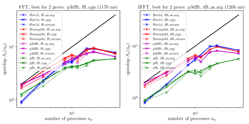
Figure 7: Speedup computed from the median of the elapsed times for 3D fft (320$\times$640$\times$640) at LEGI on cluster8.

In Fig. 7 we observe that the strong scaling for an array shape of $320\times 640\times 640$ is not far from the ideal linear trend. The fastest library is fftwmpi3d for this case. As expected from FFT algorithms, there is a slight drop in speedup when the array size is not exactly divisible by the number of processes, i.e. with 12 processes. The speedup declines rapidly when more than one node is employed (above 20 processes). This effect can be attributed to the latency introduced by inter-node communications, a hardware limitation of this cluster (10 Gb/s).

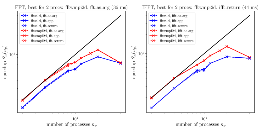
Figure 8: Speedup computed from the median of the elapsed times for 2D fft (2160$\times$2160) at LEGI on cluster8.

We have also analysed the performance of 2D MPI enabled FFT classes on the same machine using an array shaped $2160\times 2160$ in Fig. 8. The fastest library is fftwmpi2d. Both libraries display near-linear scaling, except when more than one node is used and the performance tapers off.

As a conclusive remark on scalability, a general rule of thumb should be to use 1D domain decomposition when only very few processors are employed. For massive parallelization, 2D decomposition is required to achieve good speedup without being limited by the number of processors at disposal. We have thus shown that overall performance of the libraries implemented in fft are quite good, and there is no noticeable drop in speedup when the Python API is used. This benchmark analysis also shows that the fastest FFT implementation depends on the size of the arrays and on the hardware. Therefore, an application build upon fft can be efficient for different sizes and machines.

Microbenchmark of critical “operator” functions

As already mentioned, we use Pythran (Guelton, 2018) to compile some critical “operator” functions. In this subsection, we present a microbenchmark for one simple task used in pseudo-spectral codes: projecting a velocity field on a non-divergent velocity field. It is performed in spectral space, where it can simply be written as

⬇

# pythran export proj_outplace(

# complex128[][][], complex128[][][], complex128[][][],

# float64[][][], float64[][][], float64[][][], float64[][][])

\pardef proj_outplace(vx, vy, vz, kx, ky, kz, inv_k_square_nozero):

tmp = (kx * vx + ky * vy + kz * vz) * inv_k_square_nozero

return vx - kx * tmp, vy - ky * tmp, vz - kz * tmp

Note that, this implementation is “outplace”, meaning that the result is returned by the function and that the input velocity field (vx, vy, vz) is unmodified. The comment above the function definition is a Pythran annotation, which serves as a type-hint for the variables used within the functions — all arguments being Numpy arrays in this case. Pythran needs such annotation to be able to compile this code into efficient machine instructions via a C++ code. Without Pythran the annotation has no effect, and of course, the function defaults to using Python with Numpy to execute.

The array notation is well adapted and less verbose to express this simple vector calculus. Since explicit loops with indexing is not required, the computation with Python and Numpy is not extremely slow. Despite this being quite a favourable case for Numpy, the computation with Numpy is not optimized because, internally, it involves many loops (one per arithmetic operator) and creation of temporary arrays.

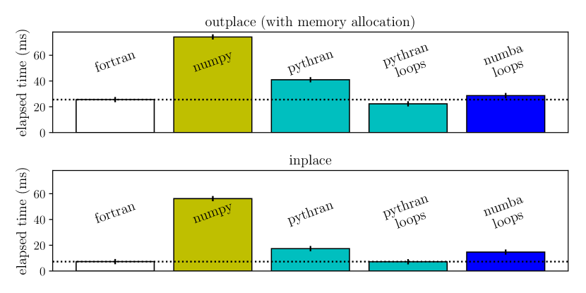
Figure 9: Elapsed time (smaller is better) for the projection function for different implementations and tools. The shape of the arrays is $(128,\ 128,\ 65)$. The dotted lines indicate the times for Fortran for better comparison.

In the top axis of Fig. 9, we compare the elapsed times for different implementations of this function. For this outplace version, we used three different codes:

1. a Fortran code (not shown) written with three nested explicit loops (one per dimension). Note that as in the Python version we also allocate the memory where the result is stored.

2. the simplest Python version shown above.

3. a Python version with three nested explicit loops:

   ⬇

   # pythran export proj_outplace_loop(

   # complex128[][][], complex128[][][], complex128[][][],

   # float64[][][], float64[][][], float64[][][], float64[][][])

   \pardef proj_outplace_loop(vx, vy, vz, kx, ky, kz, inv_k_square_nozero):

   \parrx = np.empty_like(vx)

   ry = np.empty_like(vx)

   rz = np.empty_like(vx)

   \parn0, n1, n2 = kx.shape

   \parfor i0 in range(n0):

   for i1 in range(n1):

   for i2 in range(n2):

   tmp = (kx[i0, i1, i2] * vx[i0, i1, i2]

   + ky[i0, i1, i2] * vy[i0, i1, i2]

   + kz[i0, i1, i2] * vz[i0, i1, i2]

   ) * inv_k_square_nozero[i0, i1, i2]

   \parrx[i0, i1, i2] = vx[i0, i1, i2] - kx[i0, i1, i2] * tmp

   ry[i0, i1, i2] = vz[i0, i1, i2] - kx[i0, i1, i2] * tmp

   rz[i0, i1, i2] = vy[i0, i1, i2] - kx[i0, i1, i2] * tmp

   \parreturn rx, ry, rz

For the version without explicit loops, we present the elapsed time for two cases: (i) simply using Python (yellow bar) and (ii) using the Pythranized function (first cyan bar). For the Python version with explicit loops, we only present the results for (i) the Pythranized function (second cyan bar) and (ii) the result of Numba (blue bar). We do not show the result for Numba for the code without explicit loops because it is slower than Numpy. We have also omitted the result for Numpy for the code with explicit loops because it is very inefficient. The timing is performed upon tuning the computer using the package perf.

We see that Numpy is approximately three time slower than the Fortran implementation (which as already mentioned contains the memory allocation). Just using Pythran without changing the code (first cyan bar), we save nearly 50% of the execution time but we are still significantly slower than the Fortran implementation. We reach the Fortran performance (even slightly faster) only by using Pythran with the code with explicit loops. With this code, Numba is nearly as fast (but still slower) without requiring any type annotation.

Note that the exact performance differences depend on the hardware, the software versions, the compilers and the compilation options. We use gfortran -O3 -march=native for Fortran and clang++ -O3 -march=native for Pythran.

Since allocating memory is expensive and we do not need the non-projected velocity field after the call of the function, an evident optimization is to put the output in the input arrays. Such an “in-place” version can be written with Numpy as:

⬇

# pythran export proj_inplace(

# complex128[][][], complex128[][][], complex128[][][],

# float64[][][], float64[][][], float64[][][], float64[][][])

\pardef proj_inplace(vx, vy, vz, kx, ky, kz, inv_k_square_nozero):

tmp = (kx * vx + ky * vy + kz * vz) * inv_k_square_nozero

vx -= kx * tmp

vy -= ky * tmp

vz -= kz * tmp

As in the first version, we have included the Pythran annotation. We also consider an “in-place” version with explicit loops:

⬇

# pythran export proj_inplace_loop(

# complex128[][][], complex128[][][], complex128[][][],

# float64[][][], float64[][][], float64[][][], float64[][][])

\pardef proj_inplace_loop(vx, vy, vz, kx, ky, kz, inv_k_square_nozero):

\parn0, n1, n2 = kx.shape

\parfor i0 in range(n0):

for i1 in range(n1):

for i2 in range(n2):

tmp = (kx[i0, i1, i2] * vx[i0, i1, i2]

+ ky[i0, i1, i2] * vy[i0, i1, i2]

+ kz[i0, i1, i2] * vz[i0, i1, i2]

) * inv_k_square_nozero[i0, i1, i2]

\parvx[i0, i1, i2] -= kx[i0, i1, i2] * tmp

vy[i0, i1, i2] -= ky[i0, i1, i2] * tmp

vz[i0, i1, i2] -= kz[i0, i1, i2] * tmp

\par

Note that this code is much longer and clearly less readable than the version without explicit loops. This is however the version which is used in fluidfft since it leads to faster execution.

The elapsed time for these inplace versions and for an equivalent Fortran implementation are displayed in the bottom axis of Fig. 9. The ranking is the same as for the outplace versions and Pythran is also the faster solution. However, Numpy is even more slower (7.8 times slower than Pythran with the explicit loops) than for the outplace versions.

From this short and simple microbenchmark, we can infer four main points:

• Memory allocation takes time! In Python, memory management is automatic and we tend to forget it. An important rule to write efficient code is to reuse the buffers already allocated as much as possible.

• Even for this very simple case quite favorable for Numpy (no indexing or slicing), Numpy is three to eight time slower than the Fortran implementations. As long as the execution time is small or that the function represents a small part of the total execution time, this is not an issue. However, in other cases, Python-Numpy users need to consider other solutions.

• Pythran is able to speedup the Numpy code without explicit loops and is as fast as Fortran (even slightly faster in our case) for the codes with explicit loops.

• Numba is unable to speedup the Numpy code. It gives very interesting performance for the version with explicit loops without any type annotation but the result is significantly slower than with Pythran and Fortran.

Quality control

The package fft currently supplies unit tests covering 93% of its code. These unit tests are run regularly through continuous integration on Travis CI with the most recent releases of fft’s dependencies and on Bitbucket Pipelines inside a static Docker container. The tests are run using standard Python interpreter with all supported versions.

For fft, the code coverage results are displayed at Codecov. Using third-party packages coverage and tox, it is straightforward to bootstrap the installation with dependencies, test with multiple Python versions and combine the code coverage report, ready for upload. It is also possible to run similar isolated tests using tox or coverage analysis using coverage in a local machine. Up-to-date build status and coverage status are displayed on the landing page of the Bitbucket repository. Instructions on how to run unit tests, coverage and lint tests are included in the documentation.

We also try to follow a consistent code style as recommended by PEP (Python enhancement proposals) 8 and 257. This is also inspected using lint checkers such as flake8 and pylint among the developers. The Python code is regularly cleaned up using the code formatter black.

(2) Availability

Operating system

Windows and any POSIX based OS, such as GNU/Linux and macOS.

Programming language

Python 2.7, 3.5 or above. Note that while Cython and Pythran both use the C API of CPython, fft has been successfully tested on PyPy 6.0. A C++11 supporting compiler, while not mandatory for the C++ API or Cython extensions of fft, is recommended to able to use Pythran extensions.

Dependencies

• Minimum: dyn, Numpy, Cython, and mako or Jinja2; FFTW library.

• Optional: mpi4py and Pythran; P3DFFT, PFFT and cuFFT libraries.

List of contributors

• Pierre Augier (LEGI): creator of the FluidDyn project and of fft.

• Cyrille Bonamy (LEGI): C++ code and some methods in the operator classes.

• Ashwin Vishnu Mohanan (KTH): command lines utilities, benchmarks, unit tests, continuous integration, and bug fixes.

Software location:

Name:

PyPI

Persistent identifier:

https://pypi.org/project/fluidfft

Licence:

CeCILL, a free software license adapted to both international and French legal matters, in the spirit of and retaining compatibility with the GNU General Public License (GPL).

Publisher:

Pierre Augier

Version published:

0.2.4

Date published:

02/07/2018

Code repository

Name:

Bitbucket

Persistent identifier:

https://bitbucket.org/fluiddyn/fluidfft

Licence:

CeCILL

Date published:

2017

Emulation environment

Name:

Docker

Persistent identifier:

https://hub.docker.com/r/fluiddyn/python3-stable

Licence:

CeCILL-B, a BSD compatible French licence.

Date published:

02/10/2017

Language

English

(3) Reuse potential

fft is used by the Computational Fluid Mechanics framework sim (Mohanan et al., 2018). It could be used by any C++ or Python project where real-to-complex 2D or 3D FFTs are performed.

There is no formal support mechanism. However, bug reports can be submitted at the Issues page on Bitbucket. Discussions and questions can be aired on instant messaging channels in Riot (or equivalent with Matrix protocol) or via IRC protocol on Freenode at #fluiddyn-users. Discussions can also be exchanged via the official mailing list.

Funding statement

This project has indirectly benefited from funding from the foundation Simone et Cino Del Duca de l’Institut de France, the European Research Council (ERC) under the European Union’s Horizon 2020 research and innovation program (grant agreement No 647018-WATU and Euhit consortium) and the Swedish Research Council (Vetenskapsrådet): 2013–5191. We have also been able to use supercomputers of CIMENT/GRICAD, CINES/GENCI (Grant 2018-A0040107567) and the Swedish National Infrastructure for Computing (SNIC).

Competing interests

The authors declare that they have no competing interests.

 

Copyright Notice
Authors who publish with this journal agree to the following terms:

Authors retain copyright and grant the journal right of first publication with the work simultaneously licensed under a Creative Commons Attribution License that allows others to share the work with an acknowledgement of the work’s authorship and initial publication in this journal.

Authors are able to enter into separate, additional contractual arrangements for the non-exclusive distribution of the journal’s published version of the work (e.g., post it to an institutional repository or publish it in a book), with an acknowledgement of its initial publication in this journal.

By submitting this paper you agree to the terms of this Copyright Notice, which will apply to this submission if and when it is published by this journal.

References

- (1)
- Behnel et al. (2011) Behnel, S., Bradshaw, R., Citro, C., Dalcin, L., Seljebotn, D. S. & Smith, K. (2011), ‘Cython: The Best of Both Worlds’, Computing in Science & Engineering 13(2), 31–39. doi: https://doi.org/10.1109/MCSE.2010.118.
- Cooley & Tukey (1965) Cooley, J. W. & Tukey, J. W. (1965), ‘An Algorithm for the Machine Calculation of Complex Fourier Series’, Mathematics of Computation 19(90), 297–301.
- Frigo & Johnson (2005) Frigo, M. & Johnson, S. G. (2005), ‘The design and implementation of FFTW3’, Proceedings of the IEEE 93(2), 216–231.
- Guelton (2018) Guelton, S. (2018), ‘Pythran: Crossing the Python Frontier’, Computing in Science & Engineering 20(2), 83–89.
- Mohanan et al. (2018) Mohanan, A. V., Bonamy, C. & Augier, P. (2018), ‘FluidSim: modular, object-oriented python package for high-performance CFD simulations’, J. Open Research Software (to be submitted).
- Pekurovsky (2012) Pekurovsky, D. (2012), ‘P3DFFT: A framework for parallel computations of fourier transforms in three dimensions’, SIAM Journal on Scientific Computing 34(4), C192–C209.
- Pippig (2013) Pippig, M. (2013), ‘PFFT: An extension of FFTW to massively parallel architectures’, SIAM Journal on Scientific Computing 35(3), C213–C236.