Software paper for submission to the Journal of Open Research Software

 

(1) Overview

Title

FluidSim: modular, object-oriented Python package for high-performance CFD simulations

Paper Authors

1. MOHANAN, Ashwin Vishnu^a
2. BONAMY, Cyrille^b
3. CALPE LINARES, Miguel^b
4. AUGIER, Pierre^b

^a Linné Flow Centre, Department of Mechanics, KTH, 10044 Stockholm, Sweden.
^b Univ. Grenoble Alpes, CNRS, Grenoble INP, LEGI, 38000 Grenoble, France.

Paper Author Roles and Affiliations

1. Ph.D. student, Linné Flow Centre, KTH Royal Institute of Technology, Sweden;
2. Research Engineer, LEGI, Université Grenoble Alpes, CNRS, France;
3. Ph.D. student, LEGI, Université Grenoble Alpes, CNRS, France 4. Researcher, LEGI, Université Grenoble Alpes, CNRS, France

Abstract

The Python package sim is introduced in this article as an extensible framework for Computational Fluid Mechanics (CFD) solvers. It is developed as a part of FluidDyn project (Augier et al., 2018), an effort to promote open-source and open-science collaboration within fluid mechanics community and intended for both educational as well as research purposes. Solvers in sim are scalable, High-Performance Computing (HPC) codes which are powered under the hood by the rich, scientific Python ecosystem and the Application Programming Interfaces (API) provided by dyn and fft packages (Mohanan et al., 2018). The present article describes the design aspects of sim, viz. use of Python as the main language; focus on the ease of use, reuse and maintenance of the code without compromising performance. The implementation details including optimization methods, modular organization of features and object-oriented approach of using classes to implement solvers are also briefly explained. Currently, sim includes solvers for a variety of physical problems using different numerical methods (including finite-difference methods). However, this metapaper shall dwell only on the implementation and performance of its pseudo-spectral solvers, in particular the two- and three-dimensional Navier-Stokes solvers. We investigate the performance and scalability of sim in a state of the art HPC cluster. Three similar pseudo-spectral CFD codes based on Python (Dedalus, SpectralDNS) and Fortran (NS3D) are presented and qualitatively and quantitatively compared to sim. The source code is hosted at Bitbucket as a Mercurial repository bitbucket.org/fluiddyn/fluidsim and the documentation generated using Sphinx can be read online at fluidsim.readthedocs.io.

Keywords

Python; CFD; HPC; MPI; modular; object-oriented; tested; documented; open-source

Introduction

Designed as a specialized package of the FluidDyn project for computational fluid mechanics (CFD), sim is a comprehensive solution to address the needs of a fluid mechanics student and researcher alike — by providing scalable high performance solvers, on-the-fly postprocessing, and plotting functionalities under one umbrella. In the open-science paradigm, scientists will be both users and developers of the tools at the same time. An advantage of sim is that, most of the users just have to read and write Python code. sim ensures that all critical modules, classes and functions are well documented — both as inline comments and as standalone documentation, complete with examples and tutorials. For these reasons sim can become a true collaborative code and has the potential to replace some in-house pseudo-spectral codes written in more conventional languages.

Balance between runtime efficiency and cost of development

In today’s world where clusters are moving from petascale to exascale performance, computing power is aplenty. In such a scenario, it becomes apparent that man-hours are more expensive than computing time. In other words, the cost of development outweighs the cost of computing time. Therefore, developers should be willing to make small sacrifices in efficiency, to improve development time, code maintainability and clarity in general.

For the above reasons, majority of sim’s code-base, in terms of line of code, is written using pure Python syntax. However, this is done without compromising performance, by making use of libraries such as , and optimized compilers such as Cython and Pythran.

functions and data types are sufficient for applications such as initialization and postprocessing operations, since these functions are used sparingly. Computationally intensive tasks such as time-stepping and linear algebra operators which are used in every single iteration must be offloaded to compiled extensions. This optimization strategy can be considered as the computational equivalent of the Pareto principle, also known as the 80/20 rule. The goal is to optimize such that “80 percent of the runtime is spent in 20 percent of the source code” Meyers (2012). Here, Cython (Behnel et al., 2011a) and Pythran (Guelton, 2018) compilers comes in handy. An example on how we use Pythran to reach similar performance than with Fortran by writing only Python code is described in the companion paper on fft (Mohanan et al., 2018).

The result of using such an approach is studied in the forthcoming sections by measuring the performance of sim. We will demonstrate that a very large percentage of the elapsed time is spent in the execution of optimized compiled functions and thus that the “Python cost” is negligible.

Target audiences

sim is designed to cater to the needs of three kinds of audience.

• Users, who run simulations with already available solvers. To do this, one needs to have very basic skills in Python scripting.

• Advanced users, who may extend sim by developing customized solvers for new problems by taking advantage of built-in operators and time-stepping classes. In practice, one can easily implement such solvers by changing a few methods in base solver classes. To do this, one needs to have fairly good skills in Python and in particular object-oriented programming.

• Developers, who develop the base classes, in particular, the operators and time stepping classes. One may also sometime need to write compiled extensions to improve runtime performance. To do this, desirable traits include good knowledge in Python, , Cython and Pythran.

This metapaper is intended as a short introduction to sim and its implementation, written mainly from a user-perspective. Nevertheless, we also discuss how sim can be customized and extended with minimal effort to promote code reuse. A more comprehensive and hands-on look at how to use sim can be found in the tutorials, both from a user’s and a developer’s perspective. In the latter half of the paper, we shall also inspect the performance of sim in large computing clusters and compare sim with three different pseudo-spectral CFD codes.

Implementation and architecture

New features were added over the years to the package whenever demanded by research interests, thus making the code very user-centric and function-oriented. This aspect of code development is termed as YAGNI, one of the principles of agile programming software development method, which emphasizes not to spent a lot of time developing a functionality, because most likely you aren’t gonna need it.

Almost all functionalities in sim are implemented as classes and its methods are designed to be modular and generic. This means that the user is free to use inheritance to modify certain parts to suit one’s needs, and avoiding the risk of breaking a functioning code.

Package organization

sim is meant to serve as a framework for numerical solvers using different methods. For the present version of sim there is support for finite difference and pseudo-spectral methods. An example of a finite difference solver is fluidsim.solvers.ad1d which solves the 1D advection equation. There are also solvers which do not rely on most of the base classes, such as fluidsim.base.basilisk which implements a 2D adaptive meshing solver based on the CFD code Basilisk. The collection of solvers using pseudo-spectral methods are more feature-rich in comparison.

The code is organized into the following sub-packages:

• fluidsim.base: contains all base classes and a solver for the trivial equation $\partial_{t}\mathbf{\hat{u}}=0$.

• fluidsim.operators: specialized linear algebra and numerical method operators (e.g., divergence, curl, variable transformations, dealiasing).

• fluidsim.solvers: solvers and postprocessing modules for problems such as 1D advection, 2D and 3D Navier-Stokes equations (incompressible and under the Boussinesq approximation, with and without density stratification and system rotation), one-layer shallow water and Föppl-von Kármán equations.

• fluidsim.util: utilities to load and modify an existing simulation, to test, and to benchmark a solver.

Subpackages base and operators form the backbone of this package, and are not meant to be used by the user explicitly. In practice, one can make an entirely new solver for a new problem using this framework by simply writing one or two importable files containing three classes:

• an InfoSolver class, containing the information on which classes will be used for the different tasks in the solver (time stepping, state, operators, output, etc.).

• a Simulation class describing the equations to be solved.

• a State class defining all physical variables and their spectral counterparts being solved (for example: $u_{x}$ and $u_{y}$) and methods to compute one variable from another.

We now turn our attention to the simulation object which illustrates how to access the code from the user’s perspective.

The simulation object

The simulation object is instantiated with necessary parameters just before starting the time stepping. A simple 2D Navier-Stokes simulation can be launched using the following Python script:

⬇

from fluidsim.solvers.ns2d.solver import Simul

\parparams = Simul.create_default_params()

# Modify parameters as needed

sim = Simul(params)

sim.time_stepping.start()

The script first invokes the create_default_params classmethod which returns a Parameters object, typically named params containing all default parameters. Any modifications to simulation parameters is made after this step, to meet the user’s needs. The simulation object is then instantiated by passing params as the only argument, typically named sim, ready to start the iterations.

As demonstrated above, parameters are stored in an object of the class Parameters, which uses the ParamsContainer API of dyn package Augier et al. (2018). Parameters for all possible modifications to initialization, preprocessing, forcing, time-stepping, and output of the solvers is incorporated into the object params in a hierarchial manner. Once initialized, the “public” (not hidden) API does not allow to add new parameters to this object and only modifications are permitted.

This approach is different from conventional solvers reliant on text-based input files to specify parameters, which is less robust and can cause the simulation to crash due to human errors during runtime. A similar, but less readable approach to ParamsContainer is adopted by OpenFOAM which relies on dictionaries to customize parameters. The params object can be printed on the Python or IPython console and explored interactively using tab-completion, and can be loaded from and saved into XML and HDF5 files, thus being very versatile.

Note that the same simulation object is used for the plotting and post-processing tasks. During or after the execution of a simulation, a simulation object can be created with the following code (to restart a simulation, one would rather use the function fluidsim.load_state_phys_file.):

⬇

from fluidsim import load_sim_for_plot

\par# in the directory of the simulation

sim = load_sim_for_plot()

# or with the path of the simulation

# sim = load_sim_for_plot(”~/Sim_data/NS2D.strat_240x240_S8x8_2018-04-20_13-45-54”)

\par# to retrieve the value of a parameter

print(f”viscosity = {sim.params.nu_2}”)

\par# to plot the space averaged quantities versus time

sim.output.spatial_means.plot()

# to load the corresponding data

data = sim.output.spatial_means.load()

\par# for a 2d plot of the variable ”b”

sim.output.phys_fields.plot(”b”, time=2)

# to save a 2d animation

sim.output.phys_fields.animate(”b”, tmin=1, tmax=5, save_file=True)

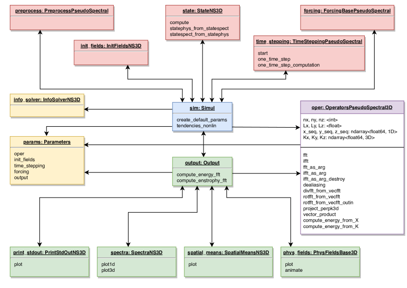
Figure 1: UML diagram of the simulation object (sim) for the solver fluidsim.solvers.ns3d. Each block represents an object or instance of a class, and the object name and the class name are written as headings. The solid arrows show how objects are associated with each other. Methods and variables of significance to the user are displayed in the body of each object block.

Fig. 1 demonstrates how an user can access different objects and its associated methods through the simulation object for the solver fluidsim.solvers.ns3d. Do note that the object and method names are similar, if not same, for other solvers. The purpose of the objects are listed below in the order of instantiation:

sim.params: A copy of the params object supplied by the user, which holds all information critical to run the simulation and generating the output. sim.info_solver: Contains all the subclass information, including the module the class belongs to. sim.info: A union of the sim.info_solver and the sim.params objects. sim.oper: Responsible for generating the grid, and for pseudo-spectral numerical methods such as FFT, IFFT, dealiasing, divergence, curl, random arrays, etc. sim.output: Takes care of all on-the-fly post-processing outputs and functions to load and plot saved output files. Different objects are assigned with tasks of loading, plotting and sometimes computing: sim.output.print_stdout: the mean energies, time elapsed and time-step of the simulation printed as console output. sim.output.phys_fields: the state variables in the physical plane. It relies on sim.state to load or compute the variables into arrays. sim.output.spatial_means: mean quantities such as energy, enstrophy, forcing power, dissipation. sim.output.spectra: energy spectra as line plots (i.e. as functions of the module or a component of the wavenumber). sim.output.spect_energy_budg: spectral energy budget by calculating the transfer term. sim.output.increments: structure functions from physical velocity fields. sim.state: Defines the names of the physical variables being solved for and their spectral equivalents, along with all required variable transformations. Also includes high-level objects, aptly named sim.state.state_phys and sim.state.state_spect to hold the arrays. sim.time_stepping: Generic numeric time-integration object which dynamically determines the time-step using the CFL criterion for specific solver and advances the state variables using Runge-Kutta method of order 2 or 4. sim.init_fields: Used only once to initialize all state variables from a previously generated output file or with simple kinds of flow structures, for example a dipole vortex, base flow with constant value for all gridpoints, grid of vortices, narrow-band noise, etc. sim.forcing: Initialized only when params.forcing.enable is set as True and it computes the forcing variables, which is added on to right-hand-side of the equations being solved. sim.preprocess: Adjusts solver parameters such as the magnitude of initialized fields, viscosity value and forcing rates after all other subclasses are initialized, and just before the time-integration starts.

Such a modular organization of the solver’s features has several advantages. The most obvious one, will be the ease of maintaining the code base. As opposed to a monolithic solver, modular codes are well separated and leads to less conflicts while merging changes from other developers. Secondly, with this implementation, it is possible to extend or replace a particular set of features by inheriting or defining a new class.

Modular codes can be difficult to navigate and understand the connection between objects and the classes in static languages. It is much less a problem with Python where one can easily decipher this information from object attributes or using IPython’s dynamic object information feature. Now, sim goes one step further and one can effortlessly print the sim.info_solver object in the Python / IPython console, to get this information. A truncated example of the output is shown below.

⬇

>>> sim.info_solver

<fluidsim.solvers.ns3d.solver.InfoSolverNS3D object at 0x7fb6278263c8>

\par<solver class_name=”Simul” module_name=”fluidsim.solvers.ns3d.solver”

short_name=”ns3d”>

<classes>

<Operators class_name=”OperatorsPseudoSpectral3D”

module_name=”fluidsim.operators.operators3d”/>

\par<State class_name=”StateNS3D” keys_computable=”[’rotz’]”

keys_linear_eigenmodes=”[’rot_fft’]” keys_phys_needed=”[’vx’, ’vy’,

’vz’]” keys_state_phys=”[’vx’, ’vy’, ’vz’]”

keys_state_spect=”[’vx_fft’, ’vy_fft’, ’vz_fft’]”

module_name=”fluidsim.solvers.ns3d.state”/>

\par<TimeStepping class_name=”TimeSteppingPseudoSpectralNS3D”

module_name=”fluidsim.solvers.ns3d.time_stepping”/>

\par<InitFields class_name=”InitFieldsNS3D”

module_name=”fluidsim.solvers.ns3d.init_fields”>

<classes>

<from_file class_name=”InitFieldsFromFile”

module_name=”fluidsim.base.init_fields”/>

\par<from_simul class_name=”InitFieldsFromSimul”

module_name=”fluidsim.base.init_fields”/>

\par<in_script class_name=”InitFieldsInScript”

module_name=”fluidsim.base.init_fields”/>

\par<constant class_name=”InitFieldsConstant”

module_name=”fluidsim.base.init_fields”/>

\par<!–truncated output–>

\par</classes>

\par</solver>

Note that while the 3D Navier-Stokes solver relies on some generic base classes, such as OperatorsPseudoSpectral3D and TimeSteppingPseudoSpectral, shared with other solvers; for other purposes there are solver specific classes. The latter is often inherited from the base classes in fluidsim.base or classes available in other solvers — this made possible by the use of an object-oriented approach. This is particularly advantageous while extending existing features or creating new solvers to use class inheritance.

Performance

Performance of a code can be carefully measured by three different program analysis methods: profiling, micro-benchmarking and scalability analysis. Profiling traces various function calls and records the cumulative time consumed and the number of calls for each function. Through profiling, we shed light on what part of the code consumes the lion’s share of the computational time and observe the impact as number of processes and MPI communications increase. Micro-benchmarking is the process of timing a specific portion of the code and comparing different implementations. The aspect is addressed in greater detail in the companion paper on fft (Mohanan et al., 2018). On the other hand, a scalability study measures how the speed of the code improves when it is deployed with multiple CPUs operating in parallel. To do this, the walltime required by the whole code is measured to complete a certain number of iterations, given a problem size. Finally, performance can also be studied by comparing different codes on representative problems. Since such comparisons should not focus only on performance, we present a comparison study in a separate section.

Cluster	Beskow (Cray XC40 system with Aries interconnect)
CPU	Intel Xeon CPU E5–2695v4, 2.1GHz
Operating System	SUSE Linux Enterprise Server 11, Linux Kernel 3.0.101
No. of cores per nodes used	32
Maximum no. of nodes used	32 (2D cases), 256 (3D cases)
Compilers	CPython 3.6.5, Intel C++ Compiler (icpc) 18.0.0
Python packages	dyn 0.2.3, fft 0.2.3, sim 0.2.1, numpy (OpenBLAS) 1.14.2, Cython 0.28.1, mpi4py 3.0.0, pythran 0.8.5

Table 1: Specifications of the supercomputing cluster and software used for profiling and benchmarking.

The profiling and scaling tests were conducted in a supercomputing cluster of the Swedish National Infrastructure for Computing (SNIC) namely Beskow (PDC, Stockholm). Relevant details regarding software and hardware which affect performance are summarised in Table 1. Note that no hyperthreading was used while carrying out the studies. The code comparisons were made on a smaller machine. Results from the three analyses are systematically studied in the following sections.

Profiling

It is straightforward to perform profiling with the help of the cProfile module, available in the Python standard library. For sim, this module has been conveniently packaged into a command line utility, fluidsim-profile. Here, we have analyzed both 2D and 3D Navier-Stokes solvers in Beskow, and plotted the results in Fig. 2 and Fig. 3 respectively. Functions which consume less than $2\%$ of the total time are displayed within a single category, other.

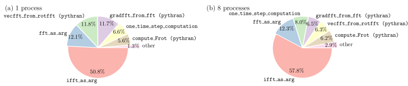
Figure 2: Profiling analysis of the 2D Navier-Stokes (fluidsim.solvers.ns2d) solver using a grid sized $1024\times 1024$ (a) in sequential with fft2d.with_fftw1d operator and (b) with 8 processes with fft2d.mpi_with_fftwmpi2d operator.

In Fig. 2 both sequential and parallel profiles of the 2D Navier-Stokes solver shows that majority of time is spent in inverse and forward FFT calls (ifft_as_arg and fft_as_arg). For the sequential case, approximately 0.14% of the time is spent in pure Python functions, i.e. functions not built using Cython and Pythran. Cython extensions are responsible for interfacing with FFT operators and also for the time-step algorithm. Pythran extensions are used to translate most of the linear algebra operations into optimized, statically compiled extensions. We also see that only 1.3% of the time is not spent in the main six functions (category other in the figure). With 8 processes deployed in parallel, time spent in pure Python function increases to 1.1% of the total time. These results show that during the optimization process, we have to focus on a very small number of functions.

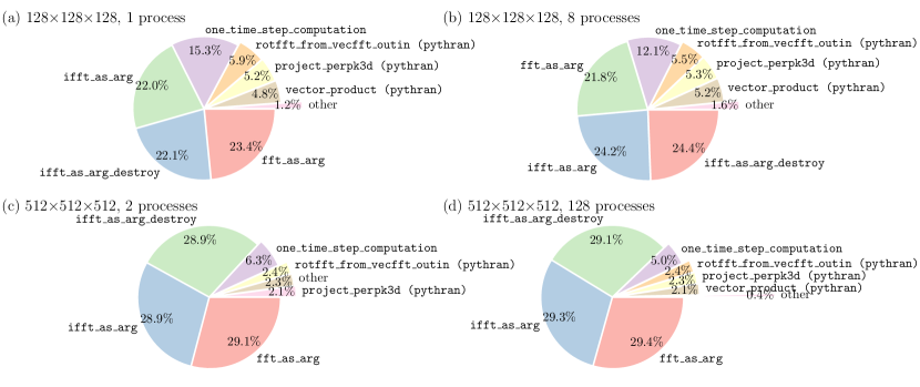
Figure 3: Profiling analysis of the 3D Navier-Stokes (fluidsim.solvers.ns3d) solver. Top row: grid sized $128\times 128\times 128$ solved (a) sequentially using fft3d.with_fftw3d operator and (b) with 8 processes using fft3d.mpi_with_fftwmpi3d operator. Bottom row: grid sized $512\times 512\times 512$ using fft3d.mpi_with_fftwmpi3d operator (c) with 2 processes and (d) with 128 processes.

From Fig. 3 it can be shown that, for the 3D Navier-Stokes solver for all cases majority of time is attributed to FFT calls. The overall time spent in pure Python function range from 0.001% for $512^{3}$ grid points and 2 processes to 0.46% for $128^{3}$ grid points and 8 processes. This percentage tends to increase with the number of processes used since the real calculation done in compiled extensions take less time. This percentage is also higher for the coarser resolution for the same reason. However, the time in pure Python remains for all cases largely negligible compared to the time spent in compiled extensions.

Scalability

Scalability can be quantified by speedup $S$ which is a measure of the time taken to complete $N$ iterations for different number of processes, $n_{p}$. We shall refrain from comparing sequential runs in this context, since the operators used for the sequential mode differ from the parallel mode, especially the FFT class. Speedup is formally defined here as:

$$S_{\alpha}(n_{p})=\frac{[\mathrm{Time\ elapsed\ for\ }N\mathrm{\ iterations\ with\ }n_{p,\min}\mathrm{\ processes}]_{\mathrm{fastest}}\times n_{p,\min}}{[\mathrm{Time\ elapsed\ for\ }N\mathrm{\ iterations\ with\ }n_{p}\mathrm{\ processes}]_{\alpha}}$$ (1)

where $n_{p,\min}$ is the minimum number of processes employed for a specific array size and hardware, $\alpha$ denotes the FFT class used and “fastest” corresponds to the fastest result among various FFT classes. In addition to number of processes, there is another important parameter, which is the size of the problem; in other words, the number of grid points used to discretize the problem at hand. In strong scaling analysis, we keep the global grid-size fixed and increase the number of processes.

Ideally, this should yield a speedup which increases linearly with number of processes. Realistically, as the number of processes increase, so does the number of MPI communications, contributing to some latency in the overall time spent and thus resulting in less than ideal performance. Also, as shown by profiling in the previous section, majority of the time is consumed in making forward- and inverse-FFT calls, an inherent bottleneck of the pseudo-spectral approach. The FFT function calls are the source of most of the MPI calls during runtime, limiting the parallelism.

2D benchmarks

The Navier-Stokes 2D solver (fluidsim.solvers.ns2d) solving an initial value problem (with random fields) was chosen as the test case for strong scaling analysis here. The physical grid was discretized with $1024\times 1024$ and $2048\times 2048$ points. Fourth-order Runge-Kutta (RK4) method with a constant time-step was used for time-integration. File input-output and the forcing term has been disabled so as to measure the performance accurately. The test case is then executed for 20 iterations. The time elapsed was measured just before and after the sim.time_stepping.start() function call, which was then utilized to calculate the average walltime per iteration and speedup. This process is repeated for two different FFT classes provided by fft, viz. fft2d.mpi_with_fftw1d and fft2d.mpi_with_fftwmpi2d.

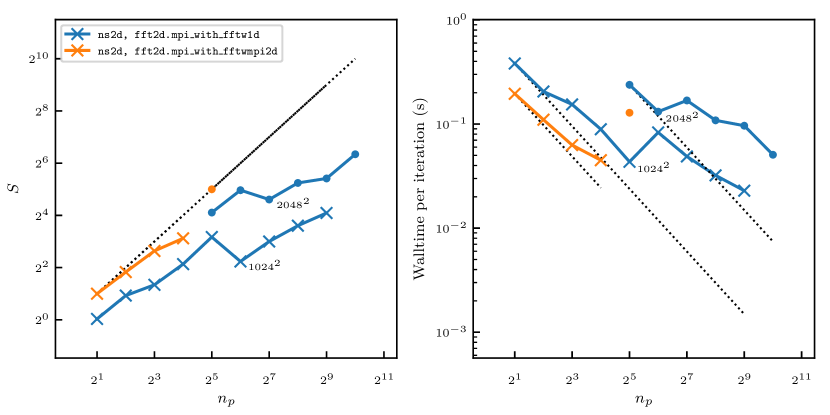
Figure 4: Strong scaling benchmarks of the 2D Navier-Stokes (fluidsim.solvers.ns2d) solver. The number of cores $n_{p}$ goes from 2 to $2^{10}=1024$. Crosses and dots correspond to $1024\times 1024$ and $2048\times 2048$ grid points, respectively.

In Fig. 4 we have analyzed the strong scaling speedup $S$ and walltime per iteration. The fastest result for a particular case is assigned the value $S=n_{p}$ as mentioned earlier in Eq. 1. Ideal speedup is indicated with a dotted black line and it varies linearly with number of processes. We notice that for the $1024\times 1024$ case there is an assured increasing trend in speedup for intra-nodes computation. Nevertheless, when this test case is solved with over a node ($n_{p}>32$); the speedup drops abruptly. While it may be argued that the speedup is impacted by the cost of inter-node MPI communications via network interfaces, that is not the case here. This is shown by speedup for the $2048\times 2048$ case, where speedup increases from $n_{p}=32$ to $64$, after which it drops again. It is thus important to remember that a decisive factor in pseudo-spectral simulations is the choice of the grid size, both global and local (per-process), and for certain shapes the FFT calls can be exceptionally fast or vice-versa.

From the above results, it may also be inferred that superior performance is achieved through the use of fft2d.mpi_with_fftwmpi2d as the FFT method. The fft2d.mpi_with_fftw1d method serves as a fallback option when either FFTW library is not compiled using MPI bindings or the domain decomposition results in zero-shaped arrays, which is a known issue with the current version of sim and requires further development.

To the right of Fig. 4, the real-time or walltime required to perform a single iteration in seconds is found to vary inversely proportional to the number of processes, $n_{p}$. The walltime per iteration ranges from $0.195$ to $0.023$ seconds for the $1024\times 1024$ case, and from $0.128$ to $0.051$ seconds for the $2048\times 2048$ case. Thus it is indeed feasible and scalable to use this particular solver.

3D benchmarks

Using a similar process as described in the previous section, the Navier-Stokes 3D solver (fluidsim.solvers.ns3d) is chosen to perform 3D benchmarks. As demonstrated in Fig. 5 two physical global grids with $128\times 128\times 128$ and $1024\times 1024\times 1024$ are used to discretize the domain. Other parameters are identical to what was described for the 2D benchmarks.

Through fft, this solver has four FFT methods at disposal:

• fft3d.mpi_with_fftw1d

• fft3d.mpi_with_fftwmpi3d

• fft3d.mpi_with_p3dfft

• fft3d.mpi_with_pfft

The first two methods implements a 1D or slab decomposition, i.e. the processes are distributed over one index of a 3D array. And the last two methods implement a 2D or pencil decomposition. For the sake of clarity, we have restricted this analysis to the fastest FFT method of the two types in this configuration, viz. fft3d.mpi_with_fftwmpi3d and fft3d.mpi_with_p3dfft. A more comprehensive study of the performance of these FFT methods can be found in Mohanan et al. (2018).

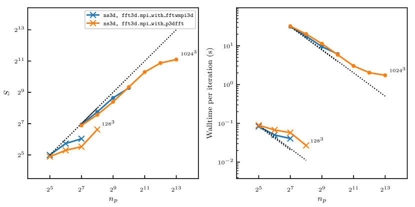
Figure 5: Strong scaling benchmarks of the 3D Navier-Stokes (fluidsim.solvers.ns3d) solver in Beskow. The number of cores $n_{p}$ goes from $2^{5}=32$ to $2^{13}=8192$. Crosses and dots correspond to $128^{3}$ and $1024^{3}$ grid points, respectively.

In Fig. 5 the strong scaling speedup and walltime per iteration are plotted from 3D benchmarks in Beskow. The analysis here is limited to single-node and inter-node performance. For both grid-sizes analyzed here, the fft3d.mpi_with_fftwmpi3d method is the fastest of all methods but limited in scalability because of the 1D domain decomposition strategy. To utilize a large number of processors, one requires the 2D decomposition approach. Also, note that for the $1024\times 1024\times 1024$ case, a single-node measurement was not possible as the size of the arrays required to run the solvers exceeds the available memory. For the same case, a speedup reasonably close to linear variation is observed with fft3d.mpi_with_p3dfft. It is also shown that the walltime per iteration improved from $0.083$ to $0.027$ seconds for the $128\times 128\times 128$ case, and from $31.078$ to $2.175$ seconds for the $1024\times 1024\times 1024$ case.

CFD pseudo-spectral code comparisons

As a general CFD framework, sim could be compared to OpenFOAM (a CFD framework based on finite-volume methods). However, in contrast to OpenFOAM, the current version of sim is highly specialized in pseudo-spectral Fourier methods and it is not adapted for industrial CFD.

In this subsection, we compare sim with three other open-source CFD pseudo-spectral codes:

• Dedalus (Burns et al., n.d.) is “a flexible framework for spectrally solving differential equations”. It is very versatile and the user describes the problem to be solved symbolically. This approach is very different than the one of sim, where the equations are described with simple code. There is no equivalent of the sim concept of a “solver”, i.e. a class corresponding to a set of equations with specialized outputs (with the corresponding plotting methods). To run a simulation with Dedalus, one has to describe the problem using mathematical equations. This can be very convenient because it is very versatile and it is not necessary to understand how Dedalus works to define a new problem. However, this approach has also drawbacks:

  • Even for very standard problems, one needs to describe the problem in the launching script.

  • There is a potentially long initialization phase during which Dedalus processes the user input and prepares the “solver”.

  • Even when a user knows how to define a problem symbolically, it is not simple to understand how the problem is solved by Dedalus and how to interact with the program with Python.

  • Since solvers are not implemented out-of-the-box in Dedalus, specialized forcing scheme or outputs are absent. For example, the user has to implement the computation, saving and plotting of standard outputs like energy spectra.

• SpectralDNS (Mortensen & Langtangen, 2016) is a “high-performance pseudo-spectral Navier-Stokes DNS solver for triply periodic domains. The most notable feature of this solver is that it is written entirely in Python using , MPI for Python (mpi4py) and pyFFTW.”

  Therefore, SpectralDNS is technically very similar to sim. Some differences are that SpectralDNS has no object oriented API, and that the user has to define output and forcing in the launching script, which are thus usually much longer than for sim. Moreover, the parallel Fourier transforms are done using the Python package mpiFFT4py, which is only able to use the FFTW library and not other libraries as with fft (Mohanan et al., 2018).

• NS3D is a highly efficient pseudo-spectral Fortran code. It has been written in the laboratory LadHyX and used for several studies involving simulations (in 3D and in 2D) of the Navier-Stokes equations under the Boussinesq approximation with stratification and system rotation Deloncle et al. (2008). It is in particular specialized in stability studies Billant et al. (2010). NS3D has been highly optimized and it is very efficient for sequential and parallel simulations (using MPI and OpenMP). However, the parallelization is limited to 1D decomposition for the FFT Mohanan et al. (2018). Another weakness compared to sim is that NS3D uses simple binary files instead of HDF5 and NetCDF4 files for sim. Therefore, visualization programs like Paraview or Visit cannot load NS3D data.

  As with many Fortran codes, Bash and Matlab are used for launching and post-processing, respectively. In terms of user experience, this can be a drawback compared to the coherent framework sim for which the user works only with Python.

  In contrast to the framework sim for which it is easy to define a new solver for a new set of equations, NS3D is specialized in solving the Navier-Stokes equations under the Boussinesq approximation. Using NS3D to solve a new set of equations would require very deep changes in many places in the code.

For quantitative comparisons and for the sake of simplicity, we limit ourselves to compare only sequential runs. We have already discussed in detail, the issue of the scalability of pseudo-spectral codes based on Fourier transforms in the previous section and in the companion paper (Mohanan et al., 2018). We compare the code with a very simple and standard task, running a solver for ten time steps with the Runge-Kutta 4 method. Note that Dedalus does not implement the standard fully explicit RK4 method. Thus for Dedalus, we use the most similar time stepping scheme available, RK443, a 4-stage, third-order mixed implicit-explicit scheme described in Ascher et al. (1997). Note that in the other codes, part of the linear terms are also treated implicitly. Also note that in several cases, the upper bound of time step is not first limited by the stability of the time scheme, rather by other needs (to resolve the fastest wave, accuracy, etc.), so these benchmarks are representative of elapsed time for accurate real-life simulations.

Bi-dimensional simulations.

	sim	Dedalus	SpectralDNS	NS3D
5122	0.54	8.01	0.92	0.82
10242	2.69	43.00	3.48	3.96

Table 2: Elapsed times (in seconds) for ten RK4 time steps for two bidimensional cases and the four CFD codes.

We first compare the elapsed times for two resolutions (512² and 1024²) over a bi-dimensional space. The results are summarized in Table 2. The results are consistent for the two resolutions. sim is the fastest code for these cases. Dedalus is more than one order of magnitude slower but as discussed earlier, the time stepping method is different. Also note that Dedalus has more been optimized for bounded domains with Chebyshev methods. The two other codes SpectralDNS and NS3D have similar performance: slightly slower than sim and much faster than Dedalus. Surprisingly, the Fortran code NS3D is slower (47%) than the Python code sim. This can be explained by the fact that there is no specialized numerical scheme for the 2D case in NS3D, so that more FFTs have to be performed compared to SpectralDNS and sim. This highlights the importance of implementing a well-adapted algorithm for a class of problems, which is much easier with a highly modular code as sim than with a specialized code as NS3D.

Tri-dimensional simulations.

We now compare the elapsed times for ten RK4 time steps for a tri-dimensional case with a resolution 128³. Dedalus is slow and does not seem to be adapted for this case so we do not give exact elapsed time for this code. SpectralDNS is slightly slower (11.55 s) than the two other codes (9.45 s for sim and 9.52 s for NS3D). This difference is mainly explained by the slower FFTs for SpectralDNS.

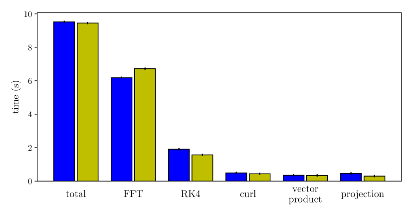
Figure 6: Comparison of the execution times for a 3D case (128³, 10 time steps) between NS3D (blue bars) and fluidsim.solvers.ns3d (yellow bars). The first two bars correspond to the total time and the others to the main tasks in terms of time consumption, namely FFT, Runge-Kutta 4, curl, vector product and “projection”.

Fig. 6 presents a more detailed comparison between NS3D (blue bars) and sim (yellow bars). The total elapsed times is mainly spent in five tasks: FFTs, Runge-Kutta 4, curl, vector product and “projection”. The times spent to perform these tasks are compared for the two codes.

We see that FFTs in NS3D are very fast: the FFT execution is 0.55 s longer for sim (nearly 9% longer). This difference is especially significant for sequential run for which there is no communication cost involved in the FFT computation, thus making it the least favorable case for sim. Indeed, MPI communications are input-output bounded tasks which are not faster in Fortran than in Python.

This difference can partially be explained by the fact that in NS3D, all FFTs are inplace (so the input can be erased during the transform). On one hand, this choice is good for performance and for a lower memory consumption. On the other hand, since the same variables are used to store the fields in real and in Fourier spaces, it makes the code harder to write, to understand and to modify. Since memory consumption in clusters is much less of a problem than in the past and that code simplicity is highly important for a framework like sim, we choose to use out-of-place FFTs in sim. Another factor is that the flag FFTW_PATIENT is used in NS3D which leads to very long initialization and sometimes faster FFTs. Since we did not see significant speed-up by using this flag in sim and that we also care about initialization time, this flag is not used and we prefer to use the flag FFTW_MEASURE, which usually leads to similar performance.

Time stepping in NS3D is significantly slower than in sim (0.34 s $\simeq$ 20 % slower). We did not find a performance issue in NS3D. The linear operators are slightly faster in sim than in the Fortran code NS3D. This is because this corresponds to Pythran functions written with explicit loops (see Mohanan et al., 2018).

Although the FFTs are a little bit faster for NS3D, the total time is slightly smaller (less than 1% of the total time) for sim for this case.

These examples do not prove that sim is always faster than NS3D or is as fast as any very well optimized Fortran codes. However, they do demonstrate that our very high-level and modular Python code is very efficient and is not slower than a well-optimized Fortran code.

Quality control

sim also packages unittests to go alongside the related modules. Throughout the development process it is made sure that all tests pass on priority to ensure that new changes to package does not damage existing functionality.

It is also important to quantify the efficacy of the tests, and this is done by calculating the code coverage. Code coverage is the ratio of the number of lines tested by unittests over the total number of lines in the whole package. For the present version of sim the code coverage is valued at approximately 60%. For sim, the code coverage results are displayed at Codecov.

We also try to follow a consistent code style as recomended by PEP (Python enhancement proposals) 8 and 257. This is also inspected using lint checkers such as flake8 and pylint among the developers. The code is regularity cleaned up using the Python code formatter black.

All the above quality control techniques are implemented within the continuous testing solutions, Travis CI and Bitbucket Pipelines. Instructions on how to run unittests, coverage and lint tests are included in the documentation.

(2) Availability

Operating system

Any POSIX based OS, such as GNU/Linux and macOS.

Programming language

Python 2.7, 3.4 or above.

Dependencies

• Minimum: dyn, , h5netcdf, fft (and FFT libraries, see Mohanan et al., 2018).

• Optional: , mpi4py, Cython and Pythran, pulp.

List of contributors

• Ashwin Vishnu Mohanan (KTH): Development of the shallow water equations solver, fluidsim.solvers.sw1l, testing, continuous integration, code coverage and documentation.

• Cyrille Bonamy (LEGI): Extending the sub-package fluidsim.operators.fft (currently deprecated) into a dedicated package, fft used by sim solvers.

• Miguel Calpe (LEGI): Development of the 2D Boussinesq equation solver, fluidsim.solvers.ns2d.strat.

• Pierre Augier (LEGI): Creator of sim and FluidDyn project, developer of majority of the modules and solvers, future-proofing with Python 3 compatibility and documentation.

Software location:

Archive

Name:

PyPI

Persistent identifier:

https://pypi.org/project/fluidsim

Licence:

CeCILL, a free software license adapted to both international and French legal matters, in the spirit of and retaining compatibility with the GNU General Public License (GPL).

Publisher:

Pierre Augier

Version published:

0.2.2

Date published:

02/07/2018

Code repository

Name:

Bitbucket

Persistent identifier:

https://bitbucket.org/fluiddyn/fluidsim

Licence:

CeCILL

Date published:

2015

Emulation environment

Name:

Docker

Persistent identifier:

https://hub.docker.com/r/fluiddyn/python3-stable

Licence:

CeCILL-B, a BSD compatible French licence.

Date published:

02/10/2017

Language

English

(3) Reuse potential

sim can be used in research and teaching to run numerical simulations with existing solvers. Its simplicity of use and its plotting capacities make it particularly adapted for teaching. sim is used at LEGI and at KTH for studies on geophysical turbulence (see for example Lindborg & Mohanan, 2017). Since it is easy to modify any characteristics of the existing solvers or to build new solvers, sim is a good tool to carry out other types of simulations for academic studies. The qualities and advantages of sim (integration with the Python ecosystem and the FluidDyn project, documentation, reliability — thanks to unittests and continuous integration —, versatility, efficiency and scalability) make us think that sim can become a true collaborative code.

There is no formal support mechanism. However, bug reports can be submitted at the Issues page on Bitbucket. Discussions and questions can be aired on instant messaging channels in Riot (or equivalent with Matrix protocol) or via IRC protocol on Freenode at #fluiddyn-users. Discussions can also be exchanged via the official mailing list.

Funding statement

This project has indirectly benefited from funding from the foundation Simone et Cino Del Duca de l’Institut de France, the European Research Council (ERC) under the European Union’s Horizon 2020 research and innovation program (grant agreement No 647018-WATU and Euhit consortium) and the Swedish Research Council (Vetenskapsrådet): 2013-5191. We have also been able to use supercomputers of CIMENT/GRICAD, CINES/GENCI and the Swedish National Infrastructure for Computing (SNIC).

Competing interests

The authors declare that they have no competing interests.

 

Copyright Notice
Authors who publish with this journal agree to the following terms:

Authors retain copyright and grant the journal right of first publication with the work simultaneously licensed under a Creative Commons Attribution License that allows others to share the work with an acknowledgement of the work’s authorship and initial publication in this journal.

Authors are able to enter into separate, additional contractual arrangements for the non-exclusive distribution of the journal’s published version of the work (e.g., post it to an institutional repository or publish it in a book), with an acknowledgement of its initial publication in this journal.

By submitting this paper you agree to the terms of this Copyright Notice, which will apply to this submission if and when it is published by this journal.

References

- (1)
- Ascher et al. (1997) Ascher, U. M., Ruuth, S. J. & Spiteri, R. J. (1997), ‘Implicit-explicit runge-kutta methods for time-dependent partial differential equations’, Applied Numerical Mathematics 25(2-3), 151–167.
- Augier et al. (2018) Augier, P., Mohanan, A. V. & Bonamy, C. (2018), ‘Fluiddyn: a python open-source framework for research and teaching in fluid dynamics’, J. Open Research Software (to be submitted).
- Behnel et al. (2011a) Behnel, S., Bradshaw, R., Citro, C., Dalcin, L., Seljebotn, D. S. & Smith, K. (2011a), ‘Cython: The Best of Both Worlds’, Computing in Science & Engineering 13(2), 31–39. doi: https://doi.org/10.1109/MCSE.2010.118.
- Behnel et al. (2011b) Behnel, S., Bradshaw, R., Citro, C., Dalcin, L., Seljebotn, D. S. & Smith, K. (2011b), ‘Cython: The best of both worlds’, Computing in Science & Engineering 13(2), 31–39.
- Billant et al. (2010) Billant, P., Deloncle, A., Chomaz, J.-M. & Otheguy, P. (2010), ‘Zigzag instability of vortex pairs in stratified and rotating fluids. part 2. analytical and numerical analyses.’, J. Fluid Mech. 660, 396–429. doi: https://doi.org/10.1017/S002211201000282X.
-
Burns et al. (n.d.)
Burns, K., Vasil, G., Oishi, J., Lecoanet, D., Brown, B. & Quataert,
E. (n.d.), ‘Dedalus: A flexible
pseudo-spectral framework for solving partial differential equations’.
https://dedalus-project.org - Deloncle et al. (2008) Deloncle, A., Billant, P. & Chomaz, J.-M. (2008), ‘Nonlinear evolution of the zigzag instability in stratified fluids: a shortcut on the route to dissipation’, Journal of Fluid Mechanics 599, 229–239.
- Guelton (2018) Guelton, S. (2018), ‘Pythran: Crossing the Python Frontier’, Computing in Science & Engineering 20(2), 83–89.
- Lindborg & Mohanan (2017) Lindborg, E. & Mohanan, A. V. (2017), ‘A two-dimensional toy model for geophysical turbulence’, Phys. Fluids 29(11), 111114. doi: https://doi.org/10.1063/1.4985990.
- Meyers (2012) Meyers, S. (2012), Effective C++ Digital Collection: 140 Ways to Improve Your Programming, Addison-Wesley.
- Mohanan et al. (2018) Mohanan, A. V., Bonamy, C. & Augier, P. (2018), ‘Fluidfft: common API (C++ and Python) for Fast Fourier Transform libraries’, J. Open Research Software (to be submitted).
- Mortensen & Langtangen (2016) Mortensen, M. & Langtangen, H. P. (2016), ‘High performance Python for direct numerical simulations of turbulent flows’, Computer Physics Communications 203(Supplement C), 53–65. doi: https://doi.org/10.1016/j.cpc.2016.02.005.