Spectral Image Classification with Deep Learning

Abstract

We present the Spectral Image Typer (SPIT), a convolutional neural network (CNN) built to classify spectral images. In contrast to traditional, rules-based algorithms which rely on meta data provided with the image (e.g. header cards), SPIT is trained solely on the image data. We have trained SPIT on 2004 human-classified images taken with the Kast spectrometer at Lick Observatory with types of Bias, Arc, Flat, Science and Standard. We include several pre-processing steps (scaling, trimming) motivated by human practice and also expanded the training set to balance between image type and increase diversity. The algorithm achieved an accuracy of 98.7% on the held-out validation set and an accuracy of 98.7% on the test set of images. We then adopt a slightly modified classification scheme to improve robustness at a modestly reduced cost in accuracy (98.2%). The majority of mis-classifications are Science frames with very faint sources confused with Arc images (e.g. faint emission line galaxies) or Science frames with very bright sources confused with Standard stars. These are errors that even a well-trained human is prone to make. Future work will increase the training set from Kast, will include additional optical and near-IR instruments, and may expand the CNN architecture complexity. We are now incorporating SPIT in the PYPIT data reduction pipeline (DRP) and are willing to facilitate its inclusion in other DRPs.

1 Introduction

The construction of an astronomical spectrum from CCD images acquired on modern facilities is a complex procedure of image processing, manipulation, extraction, and combination (e.g. Bernstein et al., 2015). This includes corrections for detector electronics and imperfections, the conversion of detector geometry to spectral (e.g. wavelength) and spatial dimensions, and the calibration of detector counts to physical flux units. To perform these steps, one generally obtains a series of calibration images that complement the on-sky, science exposures. One must then organize and associate the various types of spectral images with the science frames (prior to processing) before continuing with data reduction.

The first step in a DRP, therefore, is to identify the ‘type’ of each spectral image. The common set of spectral image types includes:

• Bias – a short exposure (ideally zero seconds) used to characterize the bias count level associated with the detector electronics.

• Dark – an exposure of finite duration, typically matched to the exposure time of the science frame, taken without any input light. This characterizes the dark current of the detector and electronics.

• Arc – a spectral image of one or more calibration arc lamps (e.g. ThAr).

• Flat – a spectral image of a continuum light source (e.g. an incandescent lamp).

• Standard – a spectral image of a bright star with a previously measured flux at the wavelengths of interest.

• Science – a spectral image of one or more science targets.

For most instruments and observatories, meta data describing the image, instrument, and telescope are saved together with the spectral image. In the Flexible Image Transport System (FITS) format, the most common format in astronomy, an ASCII Header provides this information in a series of value/comment ‘cards’. From this Header, one may develop a rules-based algorithm to decipher the meta data and thereby assign a type to the spectral image. In practice, however, this Header-based process of image-typing suffers from (i) insufficient or ambiguous information; (ii) poor human behavior (e.g. leaving the CCD shutter open when taking a dark frame); (iii) unanticipated failures of the instrument, telescope, software, or hardware (e.g. a failed arc lamp). These issues complicate image-typing and lead to erroneous processing and data reduction. A conscientious observer, therefore, tends to visually inspect each image for quality assurance and to correct the image type as needed. This laborious step is frequently performed with an image viewer and the results are manually recorded to a file (another source of human error).

Another flaw in the standard process is the specificity of rule-based algorithms. While spectral images of the same type often look very similar across instruments, there is great diversity amongst their Header data. This includes a non-uniform set of cards and values. The practice is sufficiently diverse that one cannot adopt a single code to handle all instruments (or even a pair of instruments!). Instead, one must develop a new algorithm (or parameters within that algorithm) and then test it extensively. This practice is time consuming and difficult to maintain and update.

Recognizing the challenges and loss of productivity that image-typing imposes, we have taken a deep learning approach to the problem. Recent developments in image classification with convolutional neural networks (CNNs LeCun, 1989) and our own success with classifying features in one-dimensional spectra (Parks et al., 2018), inspired our development of a CNN algorithm for spectral image-typing. In this manuscript, we report on our first results with the Spectral Image Typer (SPIT), release a product that will be expanded to include instruments across the globe, and describe the prospects for future development.

This paper is organized as follows: Section 2 presents our image training set, the CNN is described in Section 3, Section 4 reports on the validation results, and Section 5 describes future work and development. The SPIT repository is available on GitHub as part of the PYPIT organization: https://github.com/PYPIT/spit.

2 Training Set

In many respects, a CNN is only as good as its training set. For this first effort, we focus on a single instrument – the Kast spectrometer on the 3m Shane telescope of Lick Observatory. The Kast instrument is a dual camera spectrometer with one camera optimized for each of blue and red wavelengths. Kast was deployed at Lick Observatory in February 1992 and has been scheduled for nearly 5,000 nights on the Shane 3m. Figure 1 shows a fiducial set of spectral images from this instrument, labeled by image type. Co-author JXP and his collaborators have obtained thousands of spectral images with the Kast over the past several years from which we have derived the training set detailed below.

2.1 Data

We collated $\approx 3000$ images obtained on a series of observing runs of PI Prochaska and PI Hsyu from 2008 to 2016. Many of these images were typed by rules-based algorithms of the LowRedux or PYPIT DRPs and then verified by visual inspection. The latter effort was especially necessary because the Header of the blue camera was erroneous during a significant interval in this time period (e.g. incorrect specification of the calibration lamps that were off/on). From this full dataset, we selected 2004 images for training, which separate into 330 Bias images, 121 Arc frames, 777 Flat frames, 595 Science frames, and 181 Standard images. We have not included any Dark frames in this analysis.

Table 1: Training Set

Type?	Date	Frame	Usage
arc	2008-09-25	b10004	train
arc	2008-09-25	b10006	test
arc	2008-09-25	r10004	train
arc	2008-09-26	b1005	train
arc	2008-09-26	b1007	train
arc	2008-09-26	r1005	test
arc	2008-09-27	b2007	train
arc	2008-09-27	b2009	test
arc	2008-09-27	r2007	test
arc	2008-09-28	b3001	train
arc	2008-09-28	r3001	train
arc	2008-09-29	b4002	test
arc	2008-09-29	r4005	validation
arc	2010-11-05	b3000	validation
arc	2010-11-05	b3001	validation
arc	2010-11-05	b3002	train

Table 1 lists all of the images and the assigned image type. This dataset is the starting point for the training set of our CNN. From these images, we held-out 498 images for validation of the algorithm after each training iteration, as listed in the Table, and we also held-out 626 images for testing None of the validation nor test files were included in training. Each of the Kast spectral images is stored as an unsigned integer (16-bit) array in an individual FITS file. Every FITS file contains a Header, but these were entirely ignored in what follows.

Conveniently, there is significant variability within each class in the training set. The Arc frames, for example, were obtained with several grisms and gratings covering different spectral regions and with differing spectral resolutions. Furthermore, there was variation in the arc lamps employed by different observers and the exposure times adopted. Similarly, the Flat frames of the two cameras have considerably different count levels on different portions of the CCD. This variability will help force the CNN to ‘learn’ low-level features of the various image types.

Most of the spectral images obtained with Kast during this period used detectors that have the spectral dimension oriented along the detector rows, i.e. wavelengths lie along NAXIS1 in the FITS Header nomenclature and NAXIS1 $>$ NAXIS2. The few that were oriented with the spectral axis parallel to NAXIS2 were rotated 90 degrees prior to processing. As described below, we flip each image in the horizontal and vertical dimensions to increase the size and variability of the training set.

Figure 1: Example set of spectral images from the blue and red cameras of the Kast spectrometer labeled by image type. The images have been pre-processed with the zscale algorithm to emphasize spectral features.

2.2 Pre-processing

Prior to training, each input image was processed in a series of steps. Two of these steps, not coincidentally, are often performed by the human during her/his own image typing: one explict and one implicit. The implicit pre-processing step performed by a human is to ignore any large swaths of the image that are blank. Such regions result when the slit is shorter than the detector or other instrument vignetting occurs. One may also have an extensive overscan region, i.e. comparable to the size of the data region. This overscan is included in all of the spectral images, independent of type. Initially, large blank regions confused the CNN algorithm into classifying images as a Bias and we introduced a trimming pre-processing step to address this failure mode.

Figure 2: Plot of the maximum values in each row of an Arc image after performing a sigma_clip iteration. The blue dashed lines show the starting and end rows of the data region defined by our pre-processing step (see the text for further details).

We identified the data regions of our spectral images as follows. Figure 2 shows the maximum value of each row in an example Arc image (specifically frame r6 from 18 Aug 2015). To analyze the image we: (i) applied the astropy sigma_clip algorithm on the image along its zero axis (i.e. down each row). This removes any extreme outliers (e.g. cosmic ray events); (ii) iterated through each row and recorded the maximum values as displayed in the figure; (iii) iterated over the maximum value array twice, once from the front, and another time from the back. For each index value, we check if the current value is greater than the previous value by more than 10%. Bias or blank regions have count levels stable to 10% and are ignored; any large departures indicate the data region. Figure 2 indicates the region determined in this fashion and Figure 3 shows the Arc frame before and after trimming.

Figure 3: The top panel shows an Arc frame that has been scaled with zscale but is otherwise original and includes a significant, blank region in the lower 1/4 of the image. The bottom panel shows the same spectral image after trimming the empty regions from each side.

The next step in the preprocessing pipeline are to lower the image resolution. The input images are unnecessarily large and would have made the computation excessively long. Therefore, each image was resized to 210x650 pixels (spatial, spectral) using linear interpolation.

Figure 4: Example Bias image visualized before (top) and after (bottom) applying the zscale algorithm.

The explicit step taken by a human is to visualize the data with an image viewer that sets the color-map to a finite range of the flux. A popular choice to perform this rescaling is the zscale algorithm which is designed to set the color-map to span a small interval near the median value of the image. This algorithm has been applied to adjust the color-map limits for the images in Figure 1, and views with and without the scaling is shown for a Bias image in Figure 4.

Briefly, the zscale algorithm generates an interval $[z_{1},z_{2}]$ for an image $I(i)$ with $n_{\rm pix}$ flux values as:

$$z_{1}=I(i_{\rm mid})+m(1-i_{\rm mid})/C$$ (1)

$$z_{2}=I(i_{\rm mid})+m(n_{\rm pix}-i_{\rm mid})/C\;\;\;,$$ (2)

where $i_{\rm mid}$ is the central pixel of the sorted image array, $C$ is the contrast (set to 0.25), and the slope $m$ is determined by a linear function fit with iterative rejection,

$$I(i)=b+m*(i-i_{\rm mid})$$ (3)

If more than half of the points are rejected during fitting, then there is no well-defined slope and the full range of the sample defines $z_{1}$ and $z_{2}$. Finally, the image was scaled to values ranging from $0-255$ and recast as unsigned, 8-byte integers. The image may then be saved as a PNG file to disk, without the Header.

2.3 Normalization and Diversification

Out of the 2004 images in the original dataset, there was an imbalance in the various image types owing to the typical approach of astronomers to acquiring data and calibrations. This was a major issue because some of the more important classes, which are harder to distinguish from each other (e.g. Arcs from Sciences), were significantly underrepresented. Therefore, for the training and validation sets we oversampled the under-represented types and made the image count equal between all image types. This meant including additional, identical images within each of the types except Flat frames. As an example, we replicated each of the 121 Arc images six times for 756 images and then drew an additional 21 Arc images at random to match the 777 Flat frames. This yielded 3885 images across all types.

We further expanded the training set by creating three additional images by flipping the original along each axis: horizontal, vertical, and horizontal-vertical. This yielded four images per frame, including the original. This pre-processing step helps the CNN learn more effectively by forcing a more flexible algorithm and one that is forced to learn patterns instead of simply memorizing the set of images. Further work might consider randomly cropped images, or random changes to the hue, contrast and saturation.

Altogether, we had 15540 training set images that have also been scaled by zscale, trimmed to remove the overscan and any other blank regions, and resized to 210x650 pixels. Normalization and diversification (i.e. flipping) was also performed on the set of validation images yielding a total 3880 images that are classified during validation.

3 The CNN

Figure 5: Schematic of the CNN architecture that underlies SPIT. We implement two convolutional layers, each with a stride of 1, two maxpool layers each with a stride of 2, and end with a fully connected layer and a softmax classifier.

3.1 Architecture

To better describe the CNN architecture, we first define a few terms that relate to CNNs in general:

Kernel – CNNs work with filter scanners, which are NxM matrices that scan the input image and accentuate specific patterns. For our architecture, we adopted the standard 5x5 kernel that is frequently used in image processing CNNs (e.g. Inception).

Stride – Stride refers to the step-size for moving the kernel across the input image. A stride of 1 means the kernel is moved by 1 pixel in the horizontal direction, and at the end of the row it is moved 1 pixel down to continue scanning.

Depth – Depth describes the number of features that the CNN aims to learn by scanning the image. The larger the depth, the more complex features the network may learn and the more complex patterns that can be classified.

Max_pool – Max pooling refers to down sampling the original image to prevent overfitting while also enhancing the most important features. This is achieved by reducing the dimensionality of the input image. Max pooling also provides an abstracted form of the original representation. Furthermore, it reduces the computational cost by reducing the number of parameters to learn. Our architecture applies max_pool layers of 2x2 size.

Softmax classifier – Our classifier uses the softmax function which creates a probability distribution over K different outcomes. In our CNN, the softmax classifier predicts the probability of an image with respect to the five different classes. For example, an input Bias image might produce an output of [0.8, 0.1, 0.1, 0, 0], which means that the network has 80% confidence that the image is a Bias image, and 10% that it is a Science frame or a Standard frame. In a softmax function, the values range from 0 to 1 and sum to unity.

Convolutional Layer – A convolutional layer connects neurons to local regions in the input image. These layers are frequently the initial set in a CNN.

Fully Connected (FC) Layer – Unlike a Convolutional layer, the FC has all of the neurons connected to the entire previous layer. Typical practice is to use an FC layer at the end of the architecture.

One-hot encoded array – This array describes the original classes as a simple matrix. For a Bias image, the CNN represents the frame as [1, 0, 0, 0, 0], i.e.  the Bias class corresponds to the first index. The complete one-hot encoding was done as follows: 0 is Bias, 1 is Science, 2 is Standard, 3 is Arc, and 4 is a Flat frame.

The CNN we developed has the following architecture. It begins with a Convolutional Layer with a 5x5 kernel, a stride of 1 pixel, and a depth of 36. It is followed by a max_pool layer of 2x2, followed by another convolutional layer with a 5x5 kernel, a 1 pixel stride, and a depth of 64. This layer is also followed by a max_pool layer of 2x2. The architecture finishes with a fully connected layer of 128 features with a softmax classifier at the end to produce a one-hot encoded array. Figure 5 summarizes the architecture. Several, slightly modified architectures were also explored but the adopted model offered excellent performance with relatively cheap execution.

3.2 Training

For training, we used the Adam (Adaptive Moment Estimation Kingma and Ba, 2015) bundled with Google’s deep learning Tensorflow (Abadi et al., 2015) with a learning rate of $10^{-4}$ and no dropout rate. Each epoch trained on a random batch of 30 images and then was assessed against the validation image set. We ran for a series of epochs on a NVIDIA Tesla P100-SXM2 GPU, taking approximately 6s per update. After $\approx 1,000$ epochs, we noticed no significant learning. The highest accuracy achieved on the validation set during training was 98.7%, and this is the model saved for classification.

4 Results

Table 1 lists the 626 images held-out for testing the accuracy of the optimized CNN classifier. The set is comprised of 39 Arc, 103 Bias, 242 Flat, 186 Science, and 56 Standard images from the blue and red cameras of Kast. We performed several tests and assessed the overall performance of the CNN as follows.

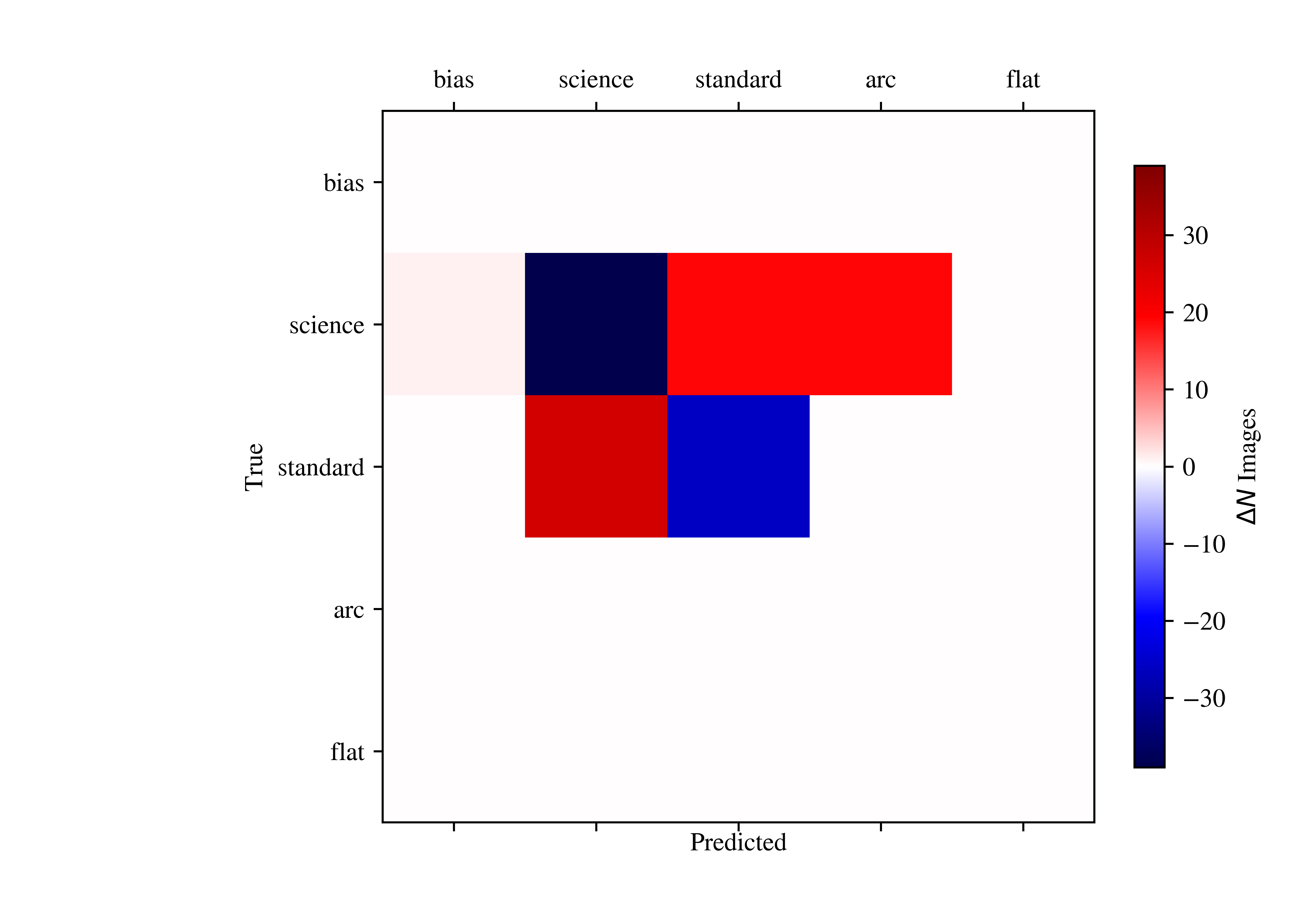
Figure 6: Differential $\Delta N$ confusion matrix describing the accuracy of the optimized CNN classifier on the normalized test suite. On the diagonal, negative values indicate the number of images that were misclassified (out of a total of 968). Off the diagonal, the positive values indicate the confusion between image types. A perfect classifier would present a differential confusion matrix of all zeros.

4.1 Normalized Accuracy

We first report results by maintaining the same methodology taken for generating the training and validation sets. Specifically, we modified the test set to have identical numbers of each image type and then assessed each of these images flipped along its horizontal and vertical axes (4 orientations for each image). Each of these was classified according to the majority value of the one-hot encoded array produced by the optimized CNN classifier.

Figure 6 shows the differential confusion matrix for this normalized test set of 4840 images. The test accuracy is 98.7%, and all of the confusion occurs for the Science and Standard frames. These results are consistent (nearly identical) to those recorded for the validation set.

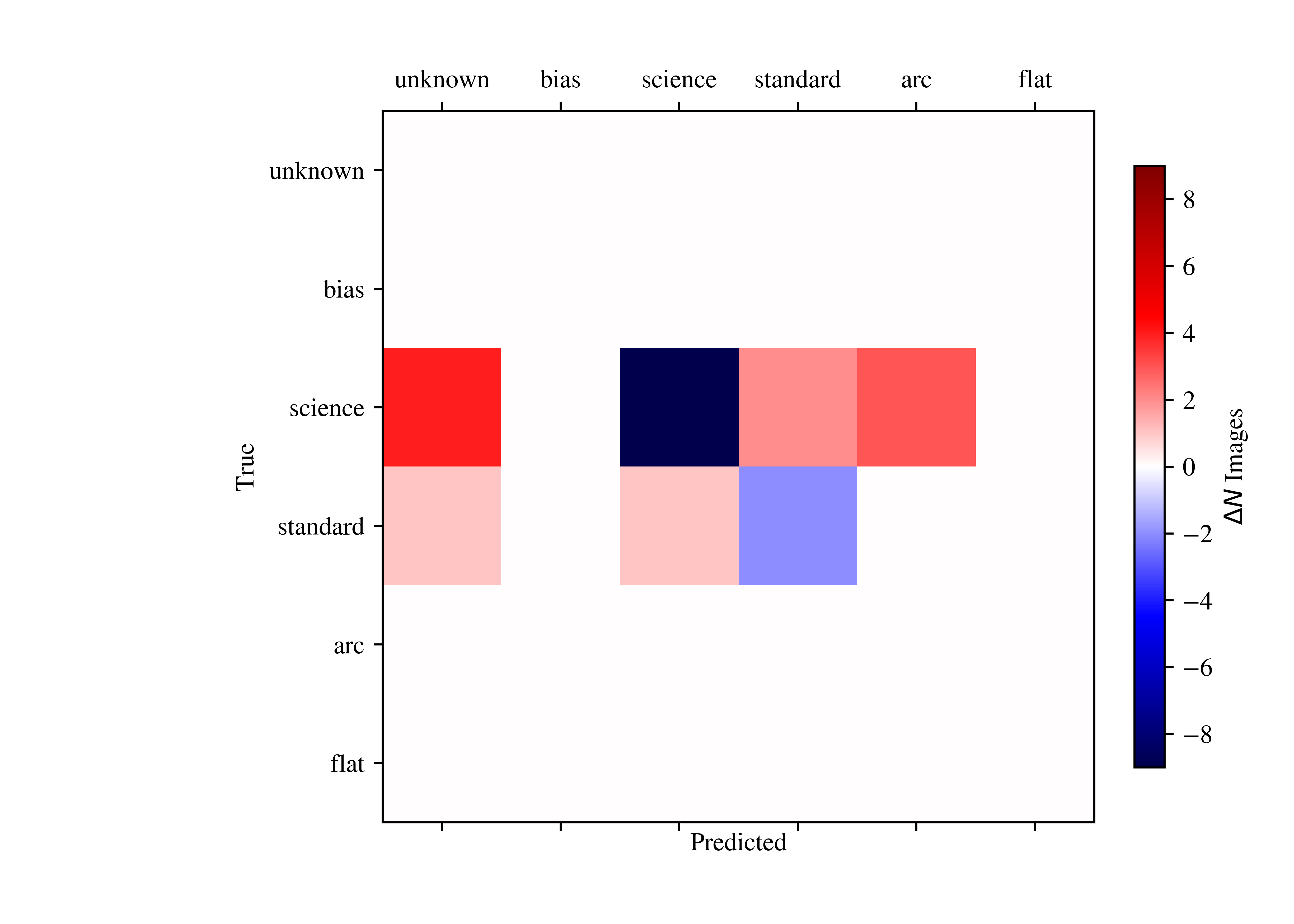
Figure 7: Differential $\Delta N$ confusion matrix describing the accuracy of the optimized CNN classifier on the test suite (unnormalized) with our final schema. On the diagonal, negative values indicate the number of images that were misclassified. Off the diagonal, the positive values indicate how the confusion between image types. A perfect classifier would present a differential confusion matrix of all zeros.

4.2 Final Accuracy

After some additional experimentation, we settled on a modified classification scheme for any unique image: (i) generate one one-hot encoded array for the input image and its three flipped counterparts; (ii) take the majority value of each one-hot encoded array; (iii) adopt the majority value of these 4 inputs provided it is a ‘super’-majority, i.e. occurring 3 or 4 times; (iv) otherwise record the classification as Unknown. This approach increases the robustness of SPIT and better identifies images that are either corrupt or especially difficult to classify based on the image data alone.

With this final schema applied to the 626 test images (i.e. without normalization), we find 98.2% are accurately classified, 0.9% were misclassified, and 0.8% were classified as Unknown. Figure 7 shows the differential confusion matrix for this final assessment.

4.3 Failures

As described above, we find that 98.2% of the test images were correctly typed, with 100% accuracy for the bias, arc, and flat image types. Our most significant set of failures are in distinguishing between Standard and Science frames. This was expected: an inexperienced human would be challenged to distinguish between these and even an experienced observer could be confused. Both may show a bright continuum trace and several sky lines. The key distinguishing characteristics are: (1) much fewer cosmic rays; (2) fainter sky-line features for the Standard frames; and (3) brighter sky continuum in the Standard frame. These are due to the shorter exposure time for Standard images and the fact that standard stars are frequently observed during twilight when the sky background from scattered sunlight is bright. We also note several mis-classifications of Science frames as Arc images. These are cases where no continuum was evident (i.e. very faint objects) and the classifier presumably confused the sky emission lines to be arc lines.

5 Future Work

Our first implementation of a CNN for spectral image typing (SPIT) has proven to be highly successful. Indeed, we are now implementing this methodology in the PYPIT DRP beginning with Kast. Future versions of SPIT will include training with images from LRIS, GMOS, HIRES, and other optical/near-IR instruments. Scientists across the country are welcome and encouraged to provide additional human-classified images for training (contact JXP).

As we expand the list to include multi-slit and echelle data, we may train a more complex CNN architecture. We will maintain all SPIT architectures online: see https://spectral-image-typing.readthedocs.io/en/latest/ for details.

References

- Abadi et al. (2015) M. Abadi, A. Agarwal, P. Barham, E. Brevdo, Z. Chen, C. Citro, G. S. Corrado, A. Davis, J. Dean, M. Devin, S. Ghemawat, I. Goodfellow, A. Harp, G. Irving, M. Isard, Y. Jia, R. Jozefowicz, L. Kaiser, M. Kudlur, J. Levenberg, D. Mané, R. Monga, S. Moore, D. Murray, C. Olah, M. Schuster, J. Shlens, B. Steiner, I. Sutskever, K. Talwar, P. Tucker, V. Vanhoucke, V. Vasudevan, F. Viégas, O. Vinyals, P. Warden, M. Wattenberg, M. Wicke, Y. Yu, and X. Zheng. TensorFlow: Large-scale machine learning on heterogeneous systems, 2015. URL http://tensorflow.org/. Software available from tensorflow.org.
- Bernstein et al. (2015) R. M. Bernstein, S. M. Burles, and J. X. Prochaska. Data Reduction with the MIKE Spectrometer. PASP, 127:911–930, Sept. 2015. 10.1086/683015.
- Kingma and Ba (2015) D. P. Kingma and J. L. Ba. Adam: a method for stochastic optimization. ICLR, 2015. URL http://arxiv.org/pdf/1412.6980.pdf.
- LeCun (1989) Y. LeCun. Generalization and network design strategies. Technical Report CRG-TR-89-4, Department of Computer Science, University of Toronto, 1989.
- Parks et al. (2018) D. Parks, J. X. Prochaska, S. Dong, and Z. Cai. Deep learning of quasar spectra to discover and characterize damped Ly systems. MNRAS, 476:1151–1168, May 2018. 10.1093/mnras/sty196.