AstroSat-CZTI detection of variable prompt emission polarization in GRB 171010A
Abstract
We present spectro-polarimetric analysis of GRB 171010A using data from AstroSat, Fermi, and Swift, to provide insights into the physical mechanisms of the prompt radiation and the jet geometry.
Prompt emission from GRB 171010A was very bright (fluence ergs cm-2) and had a complex structure composed of the superimposition of several pulses. The energy spectra deviate from the typical Band function to show a low energy peak keV — which we interpret as a power-law with two breaks, with a synchrotron origin. Alternately, the prompt spectra can also be interpreted as Comptonized emission, or a blackbody combined with a Band function. Time-resolved analysis confirms the presence of the low energy component, while the peak energy is found to be confined in the range of 100–200 keV.
Afterglow emission detected by Fermi-LAT is typical of an external shock model, and we constrain the initial Lorentz factor using the peak time of the emission. Swift-XRT measurements of the afterglow show an indication for a jet break, allowing us to constrain the jet opening angle to 6.
Detection of a large number of Compton scattered events by AstroSat-CZTI provides an opportunity to study hard X-ray polarization of the prompt emission. We find that the burst has high, time-variable polarization, with the emission have higher polarization at energies above the peak energy.
We discuss all observations in the context of GRB models and polarization arising due to due to physical or geometric effects: synchrotron emission from multiple shocks with ordered or random magnetic fields, Poynting flux dominated jet undergoing abrupt magnetic dissipation, sub-photospheric dissipation, a jet consisting of fragmented fireballs, and the Comptonization model.
1 Introduction
The emission mechanisms of gamma ray bursts (GRBs) and the radiation processes involved in producing the complex structure during the prompt phase have eluded a complete understanding in spite of the fact that these energetic cosmological events have been studied for more than five decades. Based on the duration of the observed prompt emission, GRBs are broadly classified into two families named as long and short GRBs with a demarcation at 2 s. The long GRBs are found to be associated with with type Ic supernovae pointing at their massive star origin. To extract energy efficiently to power a GRB such a collapse results in a black hole or a rapidly spinning and highly magnetized neutron star (Woosley & Bloom, 2006; Cano et al., 2017). The recent groundbreaking discovery of gravitational waves and its electromagnetic counterpart object (a short GRB) resolved the problem of identifying progenitors of short GRBs at least for the case of one joint GW/GRB detection (Abbott et al., 2016). The commonly accepted scenario for the production of the emerging radiation is based on the premise of relativistic jets being launched from the central engine. When the jet pierces through an ambient medium which is either a constant density interstellar medium (ISM) or a wind-like medium whose density varies with distance, external shocks are formed and the generated radiation has contributions from both the forward and the reverse shocks. The resultant emission constitutes the widely observed afterglows in GRBs (Rees & Meszaros, 1992; Meszaros & Rees, 1993; Mészáros & Rees, 1997; Akerlof et al., 1999; Mészáros & Rees, 1999). A plateau phase in the X-ray emission is, however, thought to be associated with a long term central engine activity or the stratification in Lorentz factor of the ejecta could also give extended energy injection (Dai & Lu, 1998; Zhang et al., 2006).
The prompt emission can arise due to various mechanisms, the leading candidates among them are: (i) increase of the jet Lorentz factor with time, leading to the collision of inner layers with the outer ones, generating internal shocks which produce non-thermal synchrotron emission as the electrons gyrate in the existing magnetic field (Narayan et al., 1992; Rees & Meszaros, 1994). A variant of internal shock model is the Internal-Collision-induced MAgnetic Reconnection and Turbulence (ICMART) model where abrupt dissipaton occurs through magnetic reconnections in a Poynting flux dominated jet (Zhang & Yan, 2011); (iii) dissipation occurring within a fuzzy photosphere; the photosphere is specially invoked to explain the quasi-thermal shape of the spectrum. The process manifests itself in such a way that it can produce a non-thermal shape of the spectrum as well (Beloborodov, 2017), (iii) gradual magnetic dissipation that occurs within the photosphere of a Poynting flux dominated jet (Beniamini & Giannios, 2017) and (iv) Comptonization of soft corona photons off the electrons present in the outgoing relativistic ejecta (Titarchuk et al., 2012; Frontera et al., 2013). These models are designed to explain the spectral properties of the prompt emission of GRBs and are successful to a certain extent. Some prominent features like the evolution of the spectral parameters and the presence of correlations among GRB observables are not well understood and most of them remain unexplained within the framework of a single model.
Another crucial information that can be added to the existing plethora of observations of the prompt emission like the spectral and timing properties, presence of afterglows, presence of associated supernovae etc, is the polarization of the prompt emission. Detection of polarization, therefore, provides an additional tool to test the theoretical models of the mechanism of GRB prompt emission. This, however, has remained a scarcely explored avenue due to the unavailability of dedicated polarimeters and reliable polarization measurements. The Cadmium Zinc Telluride Imager (CZTI) on board AstroSat, offers a new opportunity to reliably measure polarization of bright GRBs in the hard X-rays (Chattopadhyay et al., 2014; Vadawale et al., 2015; Chattopadhyay et al., 2017). The polarization expected from different models of prompt emission is not only different in magnitude but also in the expected pattern of temporal variability, depending on the emission mechanism, jet morphology and view geometry (see e.g. Covino & Gotz 2016). A study of the time variability characteristics is very important because bright GRBs whose spectra have been studied in great detail often found to have spectra deviating significantly from the standard Band function conventionally used to model the GRB spectra (Abdo et al., 2009; Izzo et al., 2012; Ackermann et al., 2010; Vianello et al., 2017; Wang et al., 2017).
GRB 171010A is a bright GRB and it presents an opportunity for a multi-pronged approach to understand the GRB prompt emission. It has been observed by both Fermi and AstroSat-CZTI. Afterglows in gamma-rays (Fermi/LAT), X-rays (Swift-XRT) and optical have been detected, and an associated supernova SN 2017htp has been found on the tenth day of the prompt emission. A redshift has been measured spectroscopically by the extended Public ESO Spectroscopic Survey for Transient Objects (ePESSTO) optical observations (Kankare et al., 2017). We present here a comprehensive analysis of this GRB using the Fermi observation for spectral properties and attempt to relate the prompt spectral properties to the detection of variable high polarization using AstroSat-CZTI. We present a summary of the observations in Section 2. The Fermi light curves and spectra are constructed in various energy bands and time bins respectively and they are presented in Sections 2, 3 and 4. The polarization measurements in different time intervals and energies are presented in Section 6. We discuss our results and derive conclusions in Section 7. The cosmological parameters chosen were , and (Komatsu et al., 2009).
2 GRB 171010A
GRB 171010A triggered the Fermi-LAT and Fermi-GBM at 19:00:50.58 UT on 2017 October 10 (Omodei et al., 2017; Poolakkil & Meegan, 2017). The observed high peak flux generated an autonomous re-point request in the GBM flight software and the Fermi telescope slewed to the GBM in-flight location. A target of opportunity observation was carried out by the Niel Gehrels Swift Observatory (Evans, 2017) and the Swift-XRT localized the burst to , and (D’Ai et al., 2017). Swift-XRT followed the burst for s111http://www.swift.ac.uk/xrt_curves/00020778/. The prompt emission was also observed by Konus-Wind (Frederiks et al., 2017). The fluence observed in the Fermi-GBM 10 - 1000 keV band from sec to s is (Poolakkil & Meegan, 2017). Here is the trigger time in the Fermi-GBM. The first photon in LAT with a probability 0.9 of its association with the source is received at s and has an energy and a photon with energy close to 1 GeV (930 MeV) is detected at s. The highest energy photon () in the Fermi-LAT is detected at . The rest frame energy of this photon is .
3 Light curves
We examined the light curves of the GRB as obtained from all 12 NaI detectors and found that detectors n7, n8 and nb (using the usual naming conventions) have significant detections (source angles are , and ). We have used data from all three detectors to examine the broad emission features of the GRB. For wide band temporal and spectral analysis, however, we chose n8 and nb, which have higher count rates than the other detectors and the angles made with the source direction for these two detectors are less than 50 degrees. The time scale used throughout this paper is relative to the Fermi-GBM trigger time . Of the two BGO scintillation detectors, the detector BGO 1 (b1), which is positioned on the same side on the satellite as the selected NaI detectors, is chosen for further analysis.
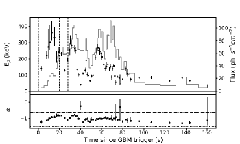
The light curve is shown in Figure 1 and it shows two episodes of emission (a) beginning at s of the main burst and lasts up to s followed by a quiescent state when the emission level meets the background level and (b) the emission becomes active again after a short period at s and radiation from the burst is detected till s. We name these emission phases as Episode 1 2. In Figure 1 we also show the light curve in the 100 - 400 keV region (the energy range of AstroSat-CZTI observations) and we use this light curve to divide the data for time resolved spectral analysis. The blocks of constant rate (Bayesian blocks) are constructed from the light curves and over-plotted on the count rate light curves to show statistically significant changes in them (Scargle et al., 2013).
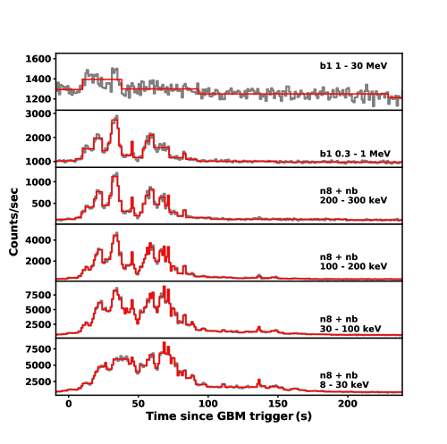
The light curves summed over the chosen GBM detectors (n8 and nb) in six different energy ranges are shown in Figure 2. The GRB has complex structure with multiple peaks and the high energy emission (above 1 MeV) is predominant till about 50 s as seen in the light curve for . Bayesian blocks are constructed from the light curves and over-plotted on the count rate.
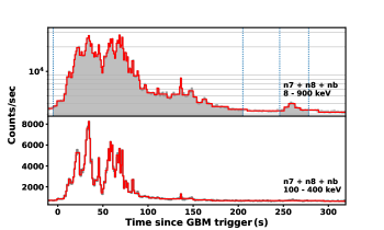
Upper Panel: Log-scale light curve in the full energy range (8 – 900 keV), binned in 1 s intervals. The two emission episodes used for time-integrated spectral analysis ( s to 205 s, 246 s to 278 s) are shaded and demarcated with vertical dotted lines. The red envelope shows the Bayesian blocks representation of the light curve.
Lower panel: Linear-scale light curve and Bayesian blocks representation for the 100 – 400 keV energy range used in time-resolved spectral analysis.
4 Spectral analysis
The burst is very bright and even with a signal to noise ratio of 50, we are able to construct more than 150 time bins. We created time bins, therefore, from the Bayesian blocks constructed from the light curve in the energy range 100 keV to 400 keV where CZTI is sensitive for polarization measurements. These bins (large number of Bayesian blocks) track significantly varying features in the lightcurve and will also be sufficient to give a substantial idea about the energetics of the burst. The spectra are reduced using Fermi Science tools software rmfit222Fermi Science Tools, rmfit: https://fermi.gsfc.nasa.gov/ssc/data/analysis/rmfit by standard methodology described in the tutorial333Fermi tutorial: https://fermi.gsfc.nasa.gov/ssc/data/analysis/scitools/rmfit_tutorial.html.
GRB prompt emission spectra generally show a typical shape described by the Band function (Band et al., 1993), however, for a number of bursts additional components are observed in the spectra such as quasi-thermal components modeled by blackbody function (Ryde, 2005; Page et al., 2011; Guiriec et al., 2011; Basak & Rao, 2015) or they show additional non-thermal components modeled by a power-law or a power-law with an exponential cut-off (Abdo et al., 2009; Ackermann et al., 2013). Additionally, for a few cases, spectra with a top-hat shape are also observed and modeled by a Band-function with an exponential roll-off at higher energies (Wang et al., 2017; Vianello et al., 2017).
The above models are driven by data and phenomenology. The physical models devised to explain the GRB prompt emission radiation have the synchrotron emission or the Compton scattering as the core processes. The synchrotron spectrum for a powerlaw distribution of electrons consists of power-laws joined at energies which depend upon cooling frequency (), minimum-injection frequency () and absorption frequency (). The Comptonization models include inverse Compton scattering as a primary mechanism (Lazzati et al., 2000; Titarchuk et al., 2012). Comptonization signatures ( grbcomp model) have been detected for a set of GRBs observed by Burst and Transient Source Experiment () on board (Frontera et al., 2013). The grbcomp model differs from the other Comptonization model: the Compton drag model. In the Compton drag model the single inverse Compton scatterings of thermal photons shape the spectrum, while in the grbcomp multiple Compton scatterings are assumed. Another major difference is that the scattering is off the outflow which is sub-relativistic in case of grbcomp model, while relativistic in the Compton drag model.
We apply this prior knowledge of spectral shapes from the previous observations of GRBs to study GRB 171010A. The spectra are modeled by various spectroscopic models available in (Arnaud, 1996). The statistics pgstat is used for optimization and testing the various models444https://heasarc.gsfc.nasa.gov/xanadu/xspec/manual/node293.html. We start with the Band function, and use the other models based upon the residuals of the data and model fit. The functional form of the Band model used to fit the photon spectrum is given in Equation 1 (Band et al., 1993),
| (1) |
Other models include blackbody555blackbody model: https://heasarc.gsfc.nasa.gov/xanadu/xspec/manual/node136.html (BB) and a power law with two breaks (bkn2pow)666bkn2pow model: https://heasarc.gsfc.nasa.gov/xanadu/xspec/manual/node141.html to model the broad band spectrum.
| (2) |
For the Comptonization model proposed by Titarchuk et al. 2012, XSPEC local model grbcomp is fit to the photon spectrum777grbcomp model: https://heasarc.nasa.gov/docs/xanadu/xspec/models//grbcomp.html. The pivotal parameters of this model are temperature of the seed blackbody spectrum (), the bulk outflow velocity of the thermal electrons (), the electron temperature of the sub-relativistic outflow (), and the energy index of the Green’s function with which the formerly Comptonized spectrum is convolved (). Using the normalization of the grbcomp model, the apparent blackbody radius can be obtained. To avoid degeneracy in the parameters or the case when parameters are difficult to constrain, we froze some of the parameters.
To fit the spectra with synchroton radiation model we implemented a table model for XSPEC. We assumed a population of electrons with a power-law energy distribution (as a result of acceleration) for , where is the minimum Lorentz factor of electrons. The cooling of electrons by synchrotron radiation is considered in slow and fast cooling regimes depending on ratio between and the cooling Lorentz factor (Sari et al., 1998). We computed the resulting photon spectrum of population of electrons assuming that the average electron distribution at a given time is for and for in fast cooling regime while for and for in slow cooling regime. The synchrotron model is made of four free parameters: the ratio between characteristic Lorentz factors , the peak energy of spectrum which is simply the energy which corresponds to the cooling frequency, the power-law index of electrons distribution p and the normalization. We built the table model for the range of and .
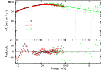
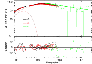
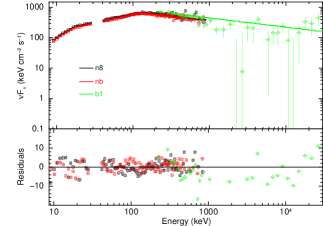
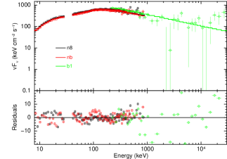
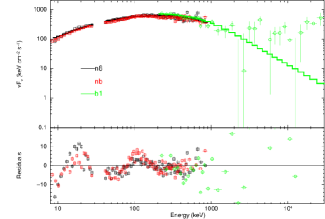
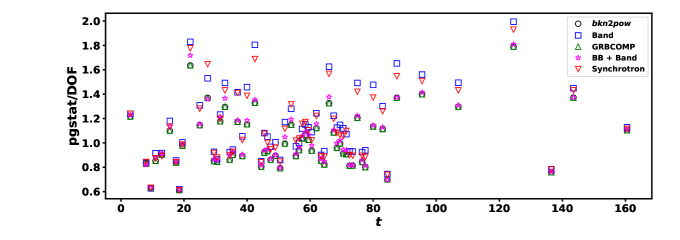
To fit the time integrated spectrum of Episode 1, we use the four models described above: (i) Band, (ii) Band + blackbody (BB), (iii) broken power law (bkn2pow), and (iv) the Comptonization model (grbcomp). The best fit parameters of the tested models are reported in Table 1. The plots, along with the residuals, are shown in Figure 3 for the four models used. The Band fit shows deviations at lower energies signifying deviations from the power law that is used to model the spectra from the low energy threshold of 8 keV to the peak energy of the Band function (150 keV). We have examined these residuals in detail by progressively raising the low energy threshold to 40 keV (greater than the energy in which the deviations are seen) and extrapolating the model to the low energies. The low energy features could still be seen. The presence of such an anomaly is found in previous studies (Tierney et al., 2013) and we conclude that a separate low energy feature in the spectra can exist. We included a blackbody (BB) along with the Band model for higher energies, but the residuals still show a systematic hump. We also tried another model for this feature of the spectrum: a powerlaw with two breaks (bkn2pow model). The bkn2pow model is preferable as the pgstat is much less for the same number of parameters (). The presence of a narrow residual hump also necessitate the need of a sharper break than a smooth blackbody curvature. This also hints that the break does not evolve much in time and thus, is not smeared out. The Comptonization model (grbcomp), however, gives the best fit for the time integrated spectrum of Episode 1. All the parameters of this model other than , fbflag and were left free. The parameter was frozen to the value to ignore terms and fbflag was set to zero to include only the first order bulk Comptonization term. A value of 3.9 for shows deviation for the seed photons from the seed blackbody spectrum. However, during the time resolved spectral analysis as reported in the next subsection we kept it fixed to 3 to consider a blackbody spectrum for the seed photons.
The isotropic energy () is calculated in the cosmological frame of the GRB by integrating the observed energy spectrum over to . The tested models differ significantly only at low energies and yield similar . We have erg for the best fit model grbcomp. The correlation between the initial Lorentz factor and the isotropic energy can be used to estimate of the fireball ejecta (Liang et al., 2010). The estimated is . The errors are propagated from the normalization and slope of the correlation. The episode 2 could be spectrally well described by a simple power-law and the best fit power-law index is for pgstat 274 for 229 degrees of freedom.
| Model | ||||||
| Band | (keV) | pgstat/dof | ||||
| BB+Band | (keV) | (keV) | pgstat/dof | |||
| 1465/333 | ||||||
| bkn2pow | (keV) | (keV) | pgstat/dof | |||
| 1421/333 | ||||||
| grbcomp | (keV) | (keV) | ( cm) | pgstat/dof | ||
| 1281/332 | ||||||
| Synchrotron model | (keV) | p | pgstat/dof | |||
4.1 Parameters evolution
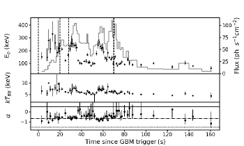
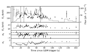
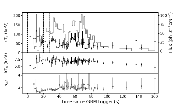
We performed time resolved analysis to capture the variations in the spectral properties by dividing the data into time segments based on the Bayesian blocks made from the 100 - 400 keV light curve. We test the models that were used for the time-integrated analysis. The deviation from Band spectrum at low energies observed in the time-integrated spectrum is also present in the time-resolved bins, thus justifying the need to use more complex models than the simple Band function. We, however, find that the three additional models (Band+BB, bknpwl, and grbcomp) represent the time resolved spectral data equally well. The evolution of the model parameters is shown in Figure 4. In Fermi-GBM, energy range 8-20 keV is divided into 12 energy channels and thus it provided sufficient data points to constrain the power-law or BB temperature whenever BB peak or low energy break falls well within these energy channels. In case of bkn2pow, the low energy index is very steep () when the break energy found to be close to the lower edge of the detection band. For such cases, we froze the index to to obtain constraints on the other parameters of the model. When we fit with the Band function, the peak energy shows three pulse like structures in their temporal evolution and these can be identified as showing a hard to soft (HTS) evolution for peaks in the photon flux. The first structure in Ep (at 10 s) can be associated with the enhancement seen in the 1 MeV flux (Figure 2, top panel). When the low energy feature is modeled using bkn2pow, almost all the peak energies fall below 200 keV. The variation in the low energy break () remains concentrated in a very narrow band ( keV). The best fit parameters for all the models are presented in Table 5.
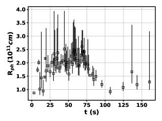
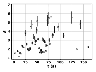
The evolution of the derived parameters of grbcomp model such as photospheric radius () and bulk parameter () is shown in Figure 6.
4.1.1 Distribution of parameters
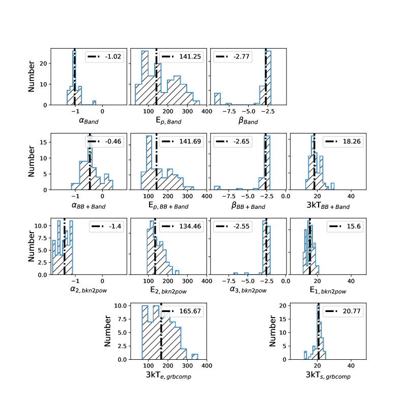
Despite the fact that the best fit to the time integrated spectrum is the Comptonization model (grbcomp), we have tested the models (i) Band, (ii) bkn2pow, (iii) BB+Band and (iv) grbcomp for the time resolved spectra. The distribution of the parameters is presented in Figure 7 and are summarized here.
For the Band function, the low energy index is distributed with a mean value . The maximum value observed is for a few time bins and in the other cases remains mostly below . The values of low energy index agree with what is typically observed for long GRBs () which is, however, known to be harder than the synchrotron radiation in the fast cooling regime. The high energy index follows a bimodal distribution with a mean value of for the major chunk concentrated around and can be interpreted as values normally observed for GRBs. The peak energy is between 32 keV and 365 keV with a median ) keV. Its distribution also shows a bimodal nature which reflects the evolution of .
In the case of bkn2pow, we observed that when the lower break energy is near the lower edge of the detection band, the power-law index below is very steep. This is expected because there are only a few channels here and the fit probably gives an unphysical result. We thus fixed the values to as they are difficult to constrain by the fits and also hamper the overall fitting process. Note that bkn2pow model is defined with an a-priori negative sign with it and we have to be cautious while comparing it with the Band function where the indices are defined without a negative sign. For the purpose of comparison we will explicitly reverse the signs of the bkn2pow indices. The mean value of is ). Here, we have ignored values 1.5 as they form another part of the bimodal distribution with low , during the time when is near the lower edge of the GBM energy band. The mean value of is . This forms the second power law from to . The third segment of the emission has power law index with a mean of . The low energy break has a mean keV and it falls in a narrow range of 11 to 20 keV. The mean is keV, comparable to the mean of Band function peak energy with a uni-modal distribution. The values are concentrated in the range 93 to 350 keV.
When a blackbody is added, the fits have an improved statistics compared to the Band function throughout the burst (see Figure 5). The blackbody temperature vary between keV with a median of keV. The distribution has harder values, while and are similar to the distributions of their counterparts in the Band function. The presence of blackbody does not seem to move the peak energies significantly, albeit an upward shift is noticeable. In the grbcomp model, the average temperature of the seed photons was 6.8 keV. The electron temperature was found to be 55 keV. We derived the photospheric radius from the normalization of the model. We found the photospheric radius cm. The grbcomp model parameters are reasonable and a photospheric radius of cm is consistent with its predictions (Frontera et al., 2013).
4.1.2 Correlations of parameters
We explore two parameter correlations and present the graphs in Figure 8.
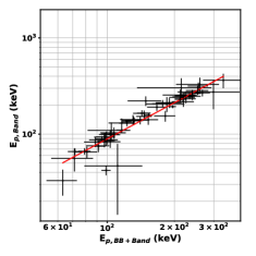
(i) vs : Thermal components observed in a set of bright Fermi single pulse GRBs are correlated to the peak of non-thermal emission (Burgess et al., 2014a). The exponent of the power-law relation () indicates the position of the photosphere if it is in the coasting phase or acceleration phase. The jet is dominated by magnetic fields when is 2 and baryonic if q is nearly 1. However, these results were found on GRBs with single pulses and for GRBs made up of overlapping pulses such criteria may not be valid. For GRB 171010A a positive correlation () between and is found with a log linear Pearson correlation coefficient of 0.81, p-value . The index points out, therefore, a magnetically dominated jet with photosphere below the saturation radius. We will discuss this result coupled with the polarization results in Section 7. The peak energy from Band function and BB + Band function are also found to be correlated, .
(ii) Correlations among grbcomp parameters: Correlations between grbcomp model parameters and other model parameters are reported in Frontera et al. (2013). We found a strong correlation between peak energy of the Band function and the bulk parameter () with log linear Pearson coefficient and p-value r(p) of -0.68 (). The seed photon temperature and photospheric radius are uncorrelated contrary to a strong anti-correlation reported in Frontera et al. 2013. The seed blackbody temperature and the electron temperature are not correlated, consistent with the predictions of grbcomp model. The parameter and peak energy of BB + Band model are correlated, with .
5 Afterglows
We have analyzed the afterglow data of GRB 171010A in gamma-rays (Fermi-LAT) and X-rays (Swift-XRT) and the results are shown in Figure 9 and 10.
5.1 -ray afterglows
A region of interest (ROI) was selected around the refined Swift-XRT coordinates and an angle of between the GRB direction and Fermi zenith was selected based on the navigation plots. The zenith cut is applied to reduce the contamination from -rays of Earth albedo. Transient event class and its instrument response function is used as it is appropriate for GRB durations. Details about LAT analysis methods and procedures can be found in the Fermi-LAT GRB catalog (Ackermann et al., 2013).
A simple power-law temporal decay is observed for the LAT light curve with a hint of momentary increase or steady emission in both energy and photon fluxes during the first and second time bins: s & s. The LAT photon flux varies with time as a power law with an index and the energy flux varies as a power law with an index . The photon index of LAT-HE is = from a spectral fit obtained by fitting the first sec data. This gives spectral index to be . The time resolved spectra do not show variation in the photon index in the first four bins.
In the external shock model, for which is generally true for reasonable shock parameters we can derive the power law index of the shocked electrons by . We have synchrotron energy flux (see the LAT lightcurve in Figure 9). We found and . The value of gives us . Thus, the power-law index for the energy flux decay can be predicted by using . The calculated value of is , which agrees well with the observed value of . Hence, we can conclude that for GRB 171010A, the LAT high energy afterglows are formed in an external forward shock.
For the thin shell case in a homogeneous medium and assuming that the peak of the LAT afterglow () occurs either before or in the second time bin gives s and we can constrain the initial Lorentz factor () of the GRB jet (see Sari & Piran 1999, Molinari et al. 2007) using
| (3) |
where is the mass of proton, is the radiation efficiency, is the time when afterglow peaks, is the k corrected rest frame energy of the GRB in the keV band. For a typical density of homogeneous ambient medium and , we can constrain the initial Lorentz factor . This limit is consistent with found in Section 4 from correlation.
The photon index hardens in the s time bin and the flux also seems to deviate from the power law fit. This hints at a contribution from an inverse Compton component. The highest energy photon with a rest frame energy of is also observed during this interval.
5.2 X-ray afterglows
The primary goal of the Swift satellite is to detect GRBs and observe the afterglows in X-ray and optical wavelengths. If a GRB is not detected by Swift but is detected by some other mission (like Fermi etc.), target of opportunity (ToO) mode observations can be initiated in Swift for very bright bursts. For such bursts the prompt phase is missed by Swift and afterglow observations are also inevitably delayed. However, the detection of X-ray afterglows with Swift-XRT not only allows us to study the delayed afterglow emissions but also to precisely localize the GRB for further ground and space based observations at longer wavelengths. The X-ray afterglow of GRB 171010A was observed by Swift s ( days) after the burst. We have used the XRT products and lightcurves from the XRT online repository888http://www.swift.ac.uk/xrt_products/index.php to study the light curve and spectral characteristics. The statistically preferred fit to the count rate light curve in the keV band has three power-law segments with two breaks. The temporal power-law indices and the break times in the light curve, as given in the GRB online repository, are listed in Table 3. The data are also consistent with 3 breaks (Table 3). The light curve with three breaks resembles the canonical GRB light curves observed in XRT (Zhang et al., 2006; Nousek et al., 2006). We have analysed the XRT spectral data and generated the energy flux light curve shown in Figure 10. The flux light curve in the 0.3 - 10 keV energy band is fit with a single powerlaw and a broken powerlaw with a single break at time . The best fit single powerlaw shows a decay index of , while in the broken powerlaw the pre- and post-break decay indices are and respectively with the break at s. These values are consistent with the fits for the count rate light curves given in Table 3.
We name the two segments of the light curve with three breaks as phase 1 (see Table 3): before and phase 2: after . The phase 1 is subjectively divided into 3 time bins to track the evolution of spectral parameters during this phase. The phase 2 is also divided at the for inspecting the spectral change with the apparent rise in the light curve after this point.
We froze the equivalent hydrogen column density () to its Galactic value (Willingale et al., 2013). Another absorption model in is used to model intrinsic absorption and corresponding to it is frozen to the value obtained from the time integrated fit. A simple power law fits the spectrum for both the phases.
The photon index in the XRT band is found to be for phase 1 and for phase 2. The evolution of energy flux in and the photon index are shown in Figure 10. Similar to LAT, it also predicts when both and evolve to energies that lie below the XRT band. If we consider (See e.g. Zhang et al. 2006, Nousek et al. 2006) which will be nearly consistent with the inferred from LAT afterglow and also near to XRT-afterglow value. Thus for the late time decay we have . When the light curve is modeled by a broken power-law, we get before the break and , thereafter. Therefore, predicted is nearly consistent with (three times the error bar). The before and after the break are consistent with the late time decay in the external shock model. And, the break observed can be identified as a jet break ( s) and used for finding the opening angle () of the jet as given by Eq. 4 (Frail et al., 2001). However, an achormatic break at all wavelengths in the lightcurves is required to claim it as a jet break. The absence of a break till the last data point observed in can also be utilized to put a lower limit on the jet break (see for example Wang et al. 2018). So any break before corresponding to last data point in XRT will also respect that limit because for a given initial Lorentz factor () the jet break will occur later for a wider jet.
| (4) |
We get () by using eq. 4. The beaming angle can be estimated by using Lorentz factor using . For , we have (). Thus, we have a wide bright jet with a narrow beaming angle. The Lorentz factor estimated above is for the final merged shells propagating to the circum-burst medium (CBM) and forming an external shock. The Lorentz factor for individual shells can even be higher than our estimate. The jet energy corrected for collimation is .
6 Polarization measurements
GRB 171010A is one of the brightest GRBs detected in CZTI with an observed fluence 10-4 erg/cm2. This makes the GRB one of potential candidates for polarization measurement. CZTI works as a Compton polarimeter where polarization is estimated from the azimuthal angle distribution of the Compton scattering events between the CZTI pixels at energies beyond 100 keV. Polarization measurement capability of CZTI has been demonstrated experimentally during its ground calibration (Chattopadhyay et al., 2014; Vadawale et al., 2015). First on board verification of its X-ray polarimetry measurement capability came with the detection of high polarization in Crab in 100 — 380 keV (Vadawale et al., 2017). Crab was observed for 800 ks in two years after its launch and this was statistically the most significant polarization measurement till date in hard X-rays. Polarimetric sensitivity of CZTI for off-axis GRBs is expected to be less than that for ON-axis sources (e.g. Crab), but the high signal to background ratio for GRBs and availability of pre-GRB and post-GRB background makes CZTI equally sensitive to polarization measurements of GRBs. Recently, we reported systematic polarization measurement for 11 GRBs, with 3 detection for 5 GRBs and 2 detection for 1 GRB, and upper limit estimation for the remaining 5 GRBs. GRB 171010A is a bright GRB registering around 2000 Compton events in CZTI. It is the second brightest GRB in terms of number of Compton events after GRB 160821A, and therefore is a potential candidate for polarization analysis.
The details of the method of polarization measurement of GRBs with CZTI can be found in Chattopadhyay et al. (2017). Here we briefly describe the different steps involved in the analysis procedure.
-
•
The first step is to identify and select the valid Compton events. We select the double pixel events during the prompt emission by identifying events happening within a 40 s time window. The double pixel events are then filtered against various Compton kinematics criteria to finally obtain the Compton scattered events.
-
•
The selection of Compton events is confined within the 33 pixel block of CZTI modules, which results in an 8 bin azimuthal scattering angle distribution. We compute the azimuthal scattering angles for events during both the GRB prompt emission and the background before and after the prompt emission. The combined pre and post-GRB azimuthal distribution is used for background subtraction to finally obtain the azimuthal distribution for the GRB.
-
•
The background corrected prompt emission azimuthal distribution shows some modulation due to (a) asymmetry in the solid angles subtended by the edge and the corner pixels to the central scattering pixel, and (b) the off-axis viewing angle of the burst. These two factors are corrected by normalizing the azimuthal angle distribution with a simulated distribution for the same GRB spectra at the same off-axis angle assuming the GRB is completely unpolarized. The simulation is performed in Geant4 with a full mass model of CZTI and AstroSat.
-
•
We fit background and geometry corrected azimuthal angle distribution using MCMC simulation to estimate the modulation factor and polarization angle (in CZTI plane). This is followed up by detailed statistical tests to determine whether the GRB is truly polarized or not. This is an important step, particularly because, there can be systematic effects which can produce significant modulation in the azimuthal angle distribution even for completely unpolarized photons. These effects are even more prominent in cases where the GRB is not very bright.
-
•
If the statistical tests suggest that the GRB is truly polarized, we estimate the polarization fraction by normalizing the fitted modulation factor with , which is the modulation factor for 100 polarized photons, obtained by simulating the GRB simulated in Geant4 with the AstroSat mass model. If the GRB is found to be unpolarized, we estimate the upper limit of polarization (see Chattopadhyay et al. (2017)).
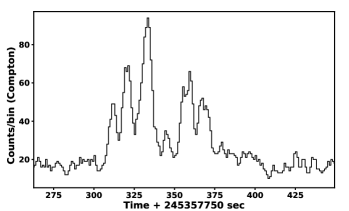
Figure 11 shows the light curve of GRB 171010A in Compton events in 100 — 300 keV. The burst is clearly seen in Compton events.
We used a total of 747 seconds of background before and after the burst for the final background estimation. After background subtraction, the number of Compton events during the prompt emission is found to be 2000. Figure 12 shows the modulation curve in the 100 — 300 keV band following background subtraction and geometry correction as discussed in the last section. We do not see any clear sinusoidal modulation in the azimuthal angle distribution.
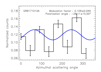
Figure 13 shows the corresponding contour plot for GRB 171010A.
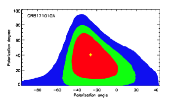
Both polarization fraction and angle are poorly constrained signifying that the burst is either unpolarized or polarization fraction is below the sensitivity level of CZTI.
In order to verify this we measure Bayes factor for sinusoidal (for polarized photons) and constant model (unpolarized photons) by utilizing ‘Thermodynamic Integration’ method on the MCMC parameter space (for details refer to Chattopadhyay et al. (2017)). This yields a value less than 2 which is assumed to be the threshold value of Bayes factor for claiming detection of polarization. We therefore estimate the upper limit of polarization for GRB 171010A which is done in two steps. First step involves estimation of polarization detection threshold (Pthr) by limiting the probability of false detection (to 0.05 for 2 or 0.01 for 3). The false polarization detection probability is estimated by simulating GRB 171010A for the observed number of Compton and background events with 100 % unpolarized photons. The second step involves measurement of the probability of detection of polarization such that probability of detection of a certain level of polarization (Pupper) being greater than the polarization detection threshold (Pthr) is 0.5 (see Chattopadhyay et al. (2017) for more details). The 2 upper limit (5 % of false detection probability) for GRB 171010A is found to be 42 . It is to be noted that in the sample of bursts used for polarization analysis in Chattopadhyay et al. (2017), GRB 160821A was found to possess maximum number of Compton events ( 2500). The next brightest burst was GRB 160623A with 1400 Compton events. We estimated 50 polarization at 3 detection significance for GRB 160821A. In comparison, GRB 171010A is found to have 2000 Compton events. The GRB is detected at an off-axis angle of 55∘. We expect CZTI to have significant polarmetric sensitivity at such off-axis angles. Therefore, polarization for this GRB should be detected at a significant detection level provided the GRB is at least 50 % polarized. This is consistent to our estimation of 2 polarization upper limit of 42 %.
This is an interesting result considering the fact that the spectral analysis suggests the time integrated peak energy for all the models is less than 200 keV which falls within the energy range of polarization analysis. Therefore, in order to see the variation of polarization below and above the peak energy, we estimate polarization in two different energy ranges — 100 — 200 keV and 200 — 300 keV (see Figure 14).
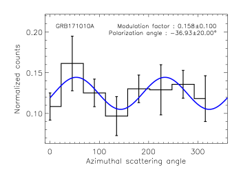
There is no clear modulation at the lower energies, whereas we see a sinusoidal variation in the modulation curve in 200 — 300 keV, which is beyond the peak energy of the GRB. However, it is to be noted that the Bayes factors for both the energy ranges are less than 2 signifying that there is no firm detection of polarization. The modulation at higher energies, therefore, is just a hint of polarization, which is still an interesting result.
One major difference between GRB 160821A (or GRB 160802A, GRB 160910A (Chattopadhyay et al., 2017)) and GRB 171010A, is that the later lasts longer and has multiple pulses. We also see significant variation of peak energy with time (see Figure 4). These pulses might exhibit different polarization signatures resulting in a net zero or low polarization when integrated in time. We therefore divided the whole burst in 3 different time intervals — 0 — 20 seconds, 20 — 28 seconds and 28 — 70 seconds, where ‘0’ is the onset of the burst. Since we have already seen a hint of polarization signature in 200 — 300 keV, we further divided the signals in 100 — 200 keV and 200 — 300 keV.


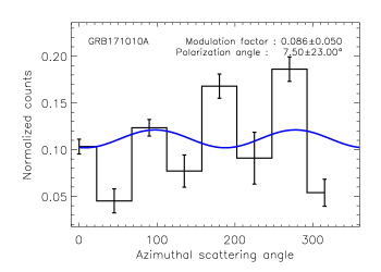
Figure 15 shows the variation of polarization fraction (middle panel), and polarization angle (bottom panel) in three time intervals for 100 — 200 keV (left) and 200 — 300 keV (right). The errors in polarization angle in the first two intervals in both the energy ranges are quite large with no significant modulation in azimuthal angle distribution consistent to being unpolarized. This is independently verified with the estimation of low values of Bayes factor. The third interval, on the other hand shows high polarization fraction with a very clear sinusoidal modulation in the azimuthal angle distribution in 200 — 300 keV (see Figure 16).
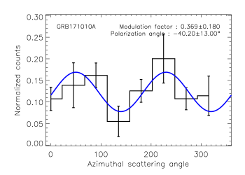
The polarization angle is also constrained within 13∘ uncertainty. The Bayes factor for this interval in 200 — 300 keV is found to be 2 with a false polarization detection probability by chance 1 % clearly signifying that the GRB is polarized at the later part of the emission at higher energies.
7 Discussions and conclusions
We presented the spectral, timing and polarization analysis of GRB 171010A which has an observed fluence . We found that the spectrum integrated over the duration of the burst is peculiar as it shows a low energy break and can be modeled by either a BB or another power law. Some GRBs have shown the presence of such a component which was modeled by a BB with peaks ranging up to 40 keV (Guiriec et al., 2011). In a comprehensive joint analysis of X-rays and higher energies in the prompt emission, a break was found in the XRT-energy window (Zheng et al., 2012; Oganesyan et al., 2018, 2017) and also in the GBM energy range (Ravasio et al., 2018). To study the detailed evolution of the spectral parameters we sliced the spectrum into multiple time bins and found that Band shows a bimodal distribution. Inclusion of a low energy component (modeled as a BB or a separate power-law) shows that the distribution of the peak energy remains keV and also falls in a concentrated region of between keV. The mean value of the break energy in the power-law with two breaks model () is keV. The power law index above the break is softer than the index obtained from the Band function. The mean value of is -1.45 and we are tempted to identify it with the synchrotron fast cooling process. can therefore be identified with the minimum energy injected to the electrons and the corresponding frequency is . On the other hand, is 0.3, harder than the value of spectral index allowed below the cooling frequency of synchrotron radiation. However, absorption frequency which can be near the GBM lower energy window has expected index to be +1, thus it is possible that the cooling frequency falls very near to the absorption frequency. In such a case can be either identified as or as the ratio or will be closer to 1. Now, relating to the fast cooling scenario can be set equal to to get the index of power-law distribution of electron energies. We get and for the distribution shown by allowed values of fall in the range 2 to 4. The component at the low energy end can also be interpreted as being of photospheric origin, generated in a region that is optically thick to the radiation, and radiation escaping at a radius where it becomes transparent. We have tested also the synchrotron model since bkn2pow gives a possibility that synchrotron model in marginally fast cooling regime could in principle work. The direct fitting of the prompt emission spectra by the synchrotron model have been performed in number of studies (Tavani, 1996; Lloyd & Petrosian, 2000; Burgess et al., 2014b; Zhang et al., 2016, 2018; Burgess et al., 2018) that give the preference to the slow or moderataly fast cooling regimes of radiation. In our analysis, the synchrotron model returns small ratio between and , and the range of pgstat/dof that is similar to other models and it has same number of parameters as Band function. Our results show that the spectral data can also be well described by a Comptonization (grbcomp) model.
From the afterglows observed in LAT (100 MeV) and XRT (0.3 -10 keV), we concluded that the afterglows are produced in an external shock propagating into the ambient medium. By assuming the ambient medium to be homogeneous, we estimated the initial Lorentz factor of the ejecta. However, the Lorentz factor thus obtained is for the merged ejecta. The sub-MeV emission possibly arises from multiple internal shocks and a stratification in the Lorentz factor can not be ruled out. From the observed break in the XRT light curve, we obtained the jet opening angle. GRB 171010A consists of a jet with initial beaming angle much narrower than the jet opening angle.
The burst shows high polarization, however significant variation in the polarization fraction (PF) and angle (PA) can be seen with energy and time. Such variations in PA can arise due to ordered magnetic field or random magnetic fields produced in shocks and when within the beaming angle, the net magnetic field can be oriented in any direction independent of the other shells. For a high polarization, the coherence length of the magnetic field () should be larger than or comparable to the beaming angle . In case of a Poynting flux dominated jet a pulse is produced in each ICMART event. The peak energy and polarisation decreases in each ICMART event. The polarisation degree and angle can vary (Zhang & Yan, 2011; Deng et al., 2016). The spectrum can be a hybrid of blackbody and Band function. We have observed a low energy feature and the spectrum deviating from Band function which was also modelled by a blackbody. This can be contribution from a photosphere (Gao & Zhang, 2015). The lower polarisation at energies below 200 keV can be due to multiple events superimposing and decreasing the net degree of polarization. The change is polarisation angle with energy also supports this argument. Therefore, the spectrum and polarization measurents are consistent with ICMART model.
In the Comptonization model multiple Compton scatterings are assumed, producing higher energy photons in the jet. The photons below the peak energy in the grbcomp model are produced by the Comptonization of the seed blackbody photons during the sub-relativistic phase. This component is, therefore, expected to be unpolarized. The high energy photons above the peak energy are mostly generated by further inverse Compton scattering off the non-thermal relativistic electrons of the relativistic outflow. This can give a polarization up to when the emission is observed at an angle with the beaming axis and unpolarized when viewed on-axis (Rybicki & Lightman, 1979). As for polarization, the highest value is expected for emission in the jet because in this case a photon, originating in the Compton cloud, illuminates the jet (or outflow) and undergoes a single up-scattering. Single scattering off jet electrons can result in a degree of polarization up to . Change in the polarization fraction and angle can be possible only if jet is fragmented and we are observing it at different viewing angles. The measured high polarization below the peak is in contradiction with the predictions of this model.
The photospheric component found in the spectra suggests that the overall spectral shape may also be explained by the sub-photospheric dissipation model (Vurm & Beloborodov, 2016). The polarization expected in the sub-photospheric dissipation model is low and tends to decrease at higher energies because the higher energy photons are produced deep within the photosphere and are reprocessed through multiple Compton scatterings before finally leaving the system at the photosphere (Lundman et al., 2016). The observed increase in the polarization with energy is in contradiction with the predictions of this model.
Another interpretation independent of the synchrotron or inverse Compton origin is that the emission is from fragmented fireballs moving with different velocity vectors (Lazzati & Begelman, 2009). The fragments moving into the direction of the observer will have the least polarization. If the intrinsic brightness of all the fragments are the same then this would also be the brightest fragment. The fragments making larger angle with the line of sight, on the other hand, will have higher polarization and lower intensity. The polarization angle can sweep randomly between different pulses in this setting. Another prediction of this geometry is that the PF and PA should not change within a single pulse. In time integrated analysis, we also find a change in polarization with energy. One possible explanation for this is that given the variability seen in the low energy light curve (100 - 200 keV), the contribution in this energy range could be from more fragments than that in the high energy light curve (200 - 300 keV). The averaging effect thus results in a relatively lower polarization fraction (maximum PF up to 100% can be achieved for the fragments viewed at , where is the Lorentz factor of a fragment) and a different position angle at lower energies in comparison to those in the high energy band. The change in polarization with time can be explained by temporally separated internal shocks produced in the different fragments. Therefore, the change in polarization from high to low seen in the 100 - 200 keV energy can be explained by considering the first pulse produced off-axis and the other brighter pulses near the axis (line of sight). In the high energy part, an increase in polarization with time is observed as well as the polarization angle are found to anti-correlate with the low energy counterpart. This suggests that the high energy emission has increased contribution with time from energetic off-axis fragments.
In the fragmented fireball scenario the jet should be fragmented into small scale (). The Lorentz factor was calculated from the LAT high energy afterglows that were produced in the external shocks. If the internal shocks were produced before the saturation in Lorentz factor was achieved then we can have a lower value of Lorentz factor when the internal shocks occur. This will allow a little room to increase . If the internal shocks are produced at small radii, then the velocity vector within the for a radially expanding ejecta will also have more divergence in their direction.
We conclude that the polarization results when used with spectral and temporal information are highly constraining. Although we cannot decisively select a single model, we find that models with a decrease in polarization with energy are either less probable or contributions from multiple underlying shocks in different energy ranges are needed to explain the apparent modulation with energy. Comptonization model has low polarization at low energies is contradiction with our observations. However independent of emission mechanisms, a geometric model consisting of multiple fragments can explain the data, but demands fragmentation at small angular scale, well within .
| Time | Index | Energy flux | Photon flux | Test Statistic |
|---|---|---|---|---|
| (s) | ( ) | ( ) | (TS) | |
| (0) 0 - 346 | (fixed) | 0 | ||
| (1) 346 - 514 | 39 | |||
| (2) 514 - 635 | 85 | |||
| (3) 635 - 1200 | 62 | |||
| (4) 1200 - 2150 | 33 | |||
| (5) 2150 - 6650 | 58 | |||
| (6) 6650 - 100000 | (fixed) | 9 |
| breaks | |||||||
|---|---|---|---|---|---|---|---|
| ( s) | ( s) | ( s) | |||||
| 1 | |||||||
| 2 | |||||||
| 3 |
| Time | Model | CSTAT/dof | ||||
|---|---|---|---|---|---|---|
| ( s) | PL | |||||
| Phase 1 | ||||||
| (2.43 - 17.5) | ||||||
| Phase 2 | 513/566 | |||||
| (17.5, 132.2) | ||||||
| Phase 1 | PL | CSTAT/dof | ||||
| (2.43, 2.58) | ||||||
| (3.03, 3.17) | ||||||
| (3.59, 4.16) | ||||||
| (13.3, 17.5) | ||||||
| Phase 2 | ||||||
| (17.5, 77.2) | ||||||
| (85, 132.2) |
| Band | ||||||||
|---|---|---|---|---|---|---|---|---|
| Sr. no. | (t1,t2) | Ep (keV) | pgstat/dof | |||||
| 1 | -1, 7 | |||||||
| 2 | 7, 9 | |||||||
| 3 | 9, 10 | |||||||
| 4 | 10, 12 | |||||||
| 5 | 12, 14 | |||||||
| 6 | 14, 17 | |||||||
| 7 | 17, 18 | |||||||
| 8 | 18, 19 | |||||||
| 9 | 19, 20 | |||||||
| 10 | 20, 24 | |||||||
| 11 | 24, 26 | |||||||
| 12 | 26, 29 | |||||||
| 13 | 29, 30 | |||||||
| 14 | 30, 31 | |||||||
| 15 | 31, 32 | |||||||
| 16 | 32, 34 | |||||||
| 17 | 34, 35 | |||||||
| 18 | 35, 36 | |||||||
| 19 | 36, 38 | |||||||
| 20 | 38, 39 | |||||||
| 21 | 39, 41 | |||||||
| 22 | 41, 44 | |||||||
| 23 | 44, 45 | |||||||
| 24 | 45, 46 | |||||||
| 25 | 46, 47 | |||||||
| 26 | 47, 48 | |||||||
| 27 | 48, 50 | |||||||
| 28 | 50, 51 | |||||||
| 29 | 51, 53 | |||||||
| 30 | 53, 55 | |||||||
| 31 | 55, 56 | |||||||
| 32 | 56, 57 | |||||||
| 33 | 57, 58 | |||||||
| 34 | 58, 59 | |||||||
| 35 | 59, 60 | |||||||
| 36 | 60, 61 | |||||||
| 37 | 61, 63 | |||||||
| 38 | 63, 64 | |||||||
| 39 | 64, 65 | |||||||
| 40 | 65, 67 | |||||||
| 41 | 67, 68 | |||||||
| 42 | 68, 69 | |||||||
| 43 | 69, 70 | |||||||
| 44 | 70, 71 | |||||||
| 45 | 71, 72 | |||||||
| 46 | 72, 73 | |||||||
| 47 | 73, 74 | |||||||
| 48 | 74, 76 | |||||||
| 49 | 76, 77 | |||||||
| 50 | 77, 78 | |||||||
| 51 | 78, 82 | |||||||
| 52 | 82, 84 | |||||||
| 53 | 84, 85 | |||||||
| 54 | 85, 90 | |||||||
| 55 | 90, 101 | |||||||
| 56 | 101, 113 | |||||||
| 57 | 113, 136 | |||||||
| 58 | 136, 137 | |||||||
| 59 | 137, 150 | |||||||
| 60 | 150, 171 | |||||||
| Broken power-law | ||||||||
| Sr. no. | (t1,t2) | (keV) | (keV) | pgstat/dof\@alignment@align | ||||
| 1 | -1, 7 | \@alignment@align | ||||||
| 2 | 7, 9 | \@alignment@align | ||||||
| 3 | 9, 10 | \@alignment@align | ||||||
| 4 | 10, 12 | \@alignment@align | ||||||
| 5 | 12, 14 | \@alignment@align |
| Broken power-law | ||||||||
|---|---|---|---|---|---|---|---|---|
| Sr. no. | (t1,t2) | (keV) | (keV) | pgstat/dof\@alignment@align | ||||
| 6 | 14, 17 | \@alignment@align | ||||||
| 7 | 17, 18 | \@alignment@align | ||||||
| 8 | 18, 19 | \@alignment@align | ||||||
| 9 | 19, 20 | \@alignment@align | ||||||
| 10 | 20, 24 | \@alignment@align | ||||||
| 11 | 24, 26 | \@alignment@align | ||||||
| 12 | 26, 29 | \@alignment@align | ||||||
| 13 | 29, 30 | \@alignment@align | ||||||
| 14 | 30, 31 | \@alignment@align | ||||||
| 15 | 31, 32 | \@alignment@align | ||||||
| 16 | 32, 34 | \@alignment@align | ||||||
| 17 | 34, 35 | \@alignment@align | ||||||
| 18 | 35, 36 | \@alignment@align | ||||||
| 19 | 36, 38 | \@alignment@align | ||||||
| 20 | 38, 39 | \@alignment@align | ||||||
| 21 | 39, 41 | \@alignment@align | ||||||
| 22 | 41, 44 | \@alignment@align | ||||||
| 23 | 44, 45 | \@alignment@align | ||||||
| 24 | 45, 46 | \@alignment@align | ||||||
| 25 | 46, 47 | \@alignment@align | ||||||
| 26 | 47, 48 | \@alignment@align | ||||||
| 27 | 48, 50 | \@alignment@align | ||||||
| 28 | 50, 51 | \@alignment@align | ||||||
| 29 | 51, 53 | \@alignment@align | ||||||
| 30 | 53, 55 | \@alignment@align | ||||||
| 31 | 55, 56 | \@alignment@align | ||||||
| 32 | 56, 57 | \@alignment@align | ||||||
| 33 | 57, 58 | \@alignment@align | ||||||
| 34 | 58, 59 | \@alignment@align | ||||||
| 35 | 59, 60 | \@alignment@align | ||||||
| 36 | 60, 61 | \@alignment@align | ||||||
| 37 | 61, 63 | \@alignment@align | ||||||
| 38 | 63, 64 | \@alignment@align | ||||||
| 39 | 64, 65 | \@alignment@align | ||||||
| 40 | 65, 67 | \@alignment@align | ||||||
| 41 | 67, 68 | \@alignment@align | ||||||
| 42 | 68, 69 | \@alignment@align | ||||||
| 43 | 69, 70 | \@alignment@align | ||||||
| 44 | 70, 71 | \@alignment@align | ||||||
| 45 | 71, 72 | \@alignment@align | ||||||
| 46 | 72, 73 | \@alignment@align | ||||||
| 47 | 73, 74 | \@alignment@align | ||||||
| 48 | 74, 76 | \@alignment@align | ||||||
| 49 | 76, 77 | \@alignment@align | ||||||
| 50 | 77, 78 | \@alignment@align | ||||||
| 51 | 78, 82 | \@alignment@align | ||||||
| 52 | 82, 84 | \@alignment@align | ||||||
| 53 | 84, 85 | \@alignment@align | ||||||
| 54 | 85, 90 | \@alignment@align | ||||||
| 55 | 90, 101 | \@alignment@align | ||||||
| 56 | 101, 113 | \@alignment@align | ||||||
| 57 | 113, 136 | \@alignment@align | ||||||
| 58 | 136, 137 | \@alignment@align | ||||||
| 59 | 137, 150 | \@alignment@align | ||||||
| 60 | 150, 171 | \@alignment@align |
: at 1 keV
| BB+Band | ||||||||
|---|---|---|---|---|---|---|---|---|
| Sr. no. | (t1,t2) | (keV) | (keV) | pgstat/dof | ||||
| 1 | -1, 7 | |||||||
| 2 | 7, 9 | |||||||
| 3 | 9, 10 | |||||||
| 4 | 10, 12 | |||||||
| 5 | 12, 14 | |||||||
| 6 | 14, 17 | |||||||
| 7 | 17, 18 | |||||||
| 8 | 18, 19 | |||||||
| 9 | 19, 20 | |||||||
| 10 | 20, 24 | |||||||
| 11 | 24, 26 | |||||||
| 12 | 26, 29 | |||||||
| 13 | 29, 30 | |||||||
| 14 | 30, 31 | |||||||
| 15 | 31, 32 | |||||||
| 16 | 32, 34 | |||||||
| 17 | 34, 35 | |||||||
| 18 | 35, 36 | |||||||
| 19 | 36, 38 | |||||||
| 20 | 38, 39 | |||||||
| 21 | 39, 41 | |||||||
| 22 | 41, 44 | |||||||
| 23 | 44, 45 | |||||||
| 24 | 45, 46 | |||||||
| 25 | 46, 47 | |||||||
| 26 | 47, 48 | |||||||
| 27 | 48, 50 | |||||||
| 28 | 50, 51 | |||||||
| 29 | 51, 53 | |||||||
| 30 | 53, 55 | |||||||
| 31 | 55, 56 | |||||||
| 32 | 56, 57 | |||||||
| 33 | 57, 58 | |||||||
| 34 | 58, 59 | |||||||
| 35 | 59, 60 | |||||||
| 36 | 60, 61 | |||||||
| 37 | 61, 63 | |||||||
| 38 | 63, 64 | |||||||
| 39 | 64, 65 | |||||||
| 40 | 65, 67 | |||||||
| 41 | 67, 68 | |||||||
| 42 | 68, 69 | |||||||
| 43 | 69, 70 | |||||||
| 44 | 70, 71 | |||||||
| 45 | 71, 72 | |||||||
| 46 | 72, 73 | |||||||
| 47 | 73, 74 | |||||||
| 48 | 74, 76 | |||||||
| 49 | 76, 77 | |||||||
| 50 | 77, 78 | |||||||
| 51 | 78, 82 | |||||||
| 52 | 82, 84 | |||||||
| 53 | 84, 85 | |||||||
| 54 | 85, 90 | |||||||
| 55 | 90, 101 | |||||||
| 56 | 101, 113 | |||||||
| 57 | 113, 136 | |||||||
| 58 | 136, 137 | |||||||
| 59 | 137, 150 | |||||||
| 60 | 150, 171 |
| grbcomp | ||||||||
|---|---|---|---|---|---|---|---|---|
| Sr. no. | (t1,t2) | (keV) | (keV) | () cm | pgstat/dof | |||
| 1 | -1, 7 | |||||||
| 2 | 7, 9 | |||||||
| 3 | 9, 10 | |||||||
| 4 | 10, 12 | |||||||
| 5 | 12, 14 | |||||||
| 6 | 14, 17 | 7 | ||||||
| 7 | 17, 18 | |||||||
| 8 | 18, 19 | |||||||
| 9 | 19, 20 | |||||||
| 10 | 20, 24 | |||||||
| 11 | 24, 26 | |||||||
| 12 | 26, 29 | |||||||
| 13 | 29, 30 | |||||||
| 14 | 30, 31 | |||||||
| 15 | 31, 32 | |||||||
| 16 | 32, 34 | |||||||
| 17 | 34, 35 | |||||||
| 18 | 35, 36 | |||||||
| 19 | 36, 38 | |||||||
| 20 | 38, 39 | |||||||
| 21 | 39, 41 | |||||||
| 22 | 41, 44 | |||||||
| 23 | 44, 45 | |||||||
| 24 | 45, 46 | |||||||
| 25 | 46, 47 | |||||||
| 26 | 47, 48 | |||||||
| 27 | 48, 50 | |||||||
| 28 | 50, 51 | |||||||
| 29 | 51, 53 | |||||||
| 30 | 53, 55 | |||||||
| 31 | 55, 56 | |||||||
| 32 | 56, 57 | |||||||
| 33 | 57, 58 | |||||||
| 34 | 58, 59 | |||||||
| 35 | 59, 60 | |||||||
| 36 | 60, 61 | |||||||
| 37 | 61, 63 | |||||||
| 38 | 63, 64 | |||||||
| 39 | 64, 65 | |||||||
| 40 | 65, 67 | |||||||
| 41 | 67, 68 | |||||||
| 42 | 68, 69 | |||||||
| 43 | 69, 70 | |||||||
| 44 | 70, 71 | |||||||
| 45 | 71, 72 | |||||||
| 46 | 72, 73 | |||||||
| 47 | 73, 74 | |||||||
| 48 | 74, 76 | |||||||
| 49 | 76, 77 | |||||||
| 50 | 77, 78 | |||||||
| 51 | 78, 82 | |||||||
| 52 | 82, 84 | |||||||
| 53 | 84, 85 | |||||||
| 54 | 85, 90 | |||||||
| 55 | 90, 101 | |||||||
| 56 | 101, 113 | |||||||
| 57 | 113, 136 | |||||||
| 58 | 136, 137 | |||||||
| 59 | 137, 150 | |||||||
| 60 | 150, 171 |
| Synchrotron model | ||||||
|---|---|---|---|---|---|---|
| Sr. no. | (t1,t2) | (keV) | p | pgstat/dof | ||
| 1 | -1, 7 | |||||
| 2 | 7, 9 | |||||
| 3 | 9, 10 | |||||
| 4 | 10, 12 | |||||
| 5 | 12, 14 | |||||
| 6 | 14, 17 | |||||
| 7 | 17, 18 | |||||
| 8 | 18, 19 | |||||
| 9 | 19, 20 | |||||
| 10 | 20, 24 | |||||
| 11 | 24, 26 | |||||
| 12 | 26, 29 | |||||
| 13 | 29, 30 | |||||
| 14 | 30, 31 | |||||
| 15 | 31, 32 | |||||
| 16 | 32, 34 | |||||
| 17 | 34, 35 | |||||
| 18 | 35, 36 | |||||
| 19 | 36, 38 | |||||
| 20 | 38, 39 | |||||
| 21 | 39, 41 | |||||
| 22 | 41, 44 | |||||
| 23 | 44, 45 | |||||
| 24 | 45, 46 | |||||
| 25 | 46, 47 | |||||
| 26 | 47, 48 | |||||
| 27 | 48, 50 | |||||
| 28 | 50, 51 | |||||
| 29 | 51, 53 | |||||
| 30 | 53, 55 | |||||
| 31 | 55, 56 | |||||
| 32 | 56, 57 | |||||
| 33 | 57, 58 | |||||
| 34 | 58, 59 | |||||
| 35 | 59, 60 | |||||
| 36 | 60, 61 | |||||
| 37 | 61, 63 | |||||
| 38 | 63, 64 | |||||
| 39 | 64, 65 | |||||
| 40 | 65, 67 | |||||
| 41 | 67, 68 | |||||
| 42 | 68, 69 | |||||
| 43 | 69, 70 | |||||
| 44 | 70, 71 | |||||
| 45 | 71, 72 | |||||
| 46 | 72, 73 | |||||
| 47 | 73, 74 | |||||
| 48 | 74, 76 | |||||
| 49 | 76, 77 | |||||
| 50 | 77, 78 | |||||
| 51 | 78, 82 | |||||
| 52 | 82, 84 | |||||
| 53 | 84, 85 | |||||
| 54 | 85, 90 | |||||
| 55 | 90, 101 | |||||
| 56 | 101, 113 | |||||
| 57 | 113, 136 | |||||
| 58 | 136, 137 | |||||
| 59 | 137, 150 | |||||
| 60 | 150, 171 |
Acknowledgements
This research has made use of data obtained through the HEASARC Online Service, provided by the NASA-GSFC, in support of NASA High Energy Astrophysics Programs. This publication also uses the data from the AstroSat mission of the Indian Space Research Organisation (ISRO), archived at the Indian Space Science Data Centre (ISSDC). CZT-Imager is built by a consortium of Institutes across India including Tata Institute of Fundamental Research, Mumbai, Vikram Sarabhai Space Centre, Thiruvananthapuram, ISRO Satellite Centre, Bengaluru, Inter University Centre for Astronomy and Astrophysics, Pune, Physical Research Laboratory, Ahmedabad, Space Application Centre, Ahmedabad: contributions from the vast technical team from all these institutes are gratefully acknowledged. The polarimetric computations were performed on the HPC resources at the Physical Research Laboratory (PRL). We thank Lev Titarchuk for discussions on the model.
References
- Abbott et al. (2016) Abbott, B. P., Abbott, R., Abbott, T. D., et al. 2016, Physical Review Letters, 116, 061102
- Abdo et al. (2009) Abdo, A. A., Ackermann, M., Ajello, M., et al. 2009, ApJ, 706, L138
- Ackermann et al. (2010) Ackermann, M., Asano, K., Atwood, W. B., et al. 2010, ApJ, 716, 1178
- Ackermann et al. (2013) Ackermann, M., Ajello, M., Asano, K., et al. 2013, ApJS, 209, 11
- Akerlof et al. (1999) Akerlof, C., Balsano, R., Barthelmy, S., et al. 1999, Nature, 398, 400
- Arnaud (1996) Arnaud, K. A. 1996, in Astronomical Society of the Pacific Conference Series, Vol. 101, Astronomical Data Analysis Software and Systems V, ed. G. H. Jacoby & J. Barnes, 17
- Band et al. (1993) Band, D., Matteson, J., Ford, L., et al. 1993, ApJ, 413, 281
- Basak & Rao (2015) Basak, R., & Rao, A. R. 2015, ApJ, 812, 156
- Beloborodov (2017) Beloborodov, A. M. 2017, ApJ, 838, 125
- Beniamini & Giannios (2017) Beniamini, P., & Giannios, D. 2017, MNRAS, 468, 3202
- Burgess et al. (2018) Burgess, J. M., Bégué, D., Bacelj, A., et al. 2018, arXiv e-prints, arXiv:1810.06965
- Burgess et al. (2014a) Burgess, J. M., Preece, R. D., Ryde, F., et al. 2014a, ApJ, 784, L43
- Burgess et al. (2014b) Burgess, J. M., Preece, R. D., Connaughton, V., et al. 2014b, ApJ, 784, 17
- Cano et al. (2017) Cano, Z., Wang, S.-Q., Dai, Z.-G., & Wu, X.-F. 2017, Advances in Astronomy, 2017, 8929054
- Chattopadhyay et al. (2014) Chattopadhyay, T., Vadawale, S. V., Rao, A. R., Sreekumar, S., & Bhattacharya, D. 2014, Experimental Astronomy, 37, 555
- Chattopadhyay et al. (2017) Chattopadhyay, T., Vadawale, S. V., Aarthy, E., et al. 2017, ArXiv e-prints, arXiv:1707.06595
- Covino & Gotz (2016) Covino, S., & Gotz, D. 2016, Astronomical and Astrophysical Transactions, 29, 205
- D’Ai et al. (2017) D’Ai, A., Melandri, A., Sbarufatti, B., et al. 2017, GRB Coordinates Network, Circular Service, No. 21989, #1-2018 (2017), 21989
- Dai & Lu (1998) Dai, Z. G., & Lu, T. 1998, A&A, 333, L87
- Deng et al. (2016) Deng, W., Zhang, H., Zhang, B., & Li, H. 2016, ApJ, 821, L12
- Evans (2017) Evans, P. A. 2017, GRB Coordinates Network, Circular Service, No. 21986, #1-2018 (2017), 21986
- Frail et al. (2001) Frail, D. A., Kulkarni, S. R., Sari, R., et al. 2001, ApJ, 562, L55
- Frederiks et al. (2017) Frederiks, D., Golenetskii, S., Aptekar, R., et al. 2017, GRB Coordinates Network, Circular Service, No. 22003, #1-2018 (2017), 22003
- Frontera et al. (2013) Frontera, F., Amati, L., Farinelli, R., et al. 2013, ApJ, 779, 175
- Gao & Zhang (2015) Gao, H., & Zhang, B. 2015, ApJ, 801, 103
- Guiriec et al. (2011) Guiriec, S., Connaughton, V., Briggs, M. S., et al. 2011, ApJ, 727, L33
- Izzo et al. (2012) Izzo, L., Ruffini, R., Penacchioni, A. V., et al. 2012, A&A, 543, A10
- Kankare et al. (2017) Kankare, E., O’Neill, D., Izzo, L., et al. 2017, GRB Coordinates Network, Circular Service, No. 22002, #1-2018 (2017), 22002
- Komatsu et al. (2009) Komatsu, E., Dunkley, J., Nolta, M. R., et al. 2009, ApJS, 180, 330
- Lazzati & Begelman (2009) Lazzati, D., & Begelman, M. C. 2009, ApJ, 700, L141
- Lazzati et al. (2000) Lazzati, D., Ghisellini, G., Celotti, A., & Rees, M. J. 2000, ApJ, 529, L17
- Liang et al. (2010) Liang, E.-W., Yi, S.-X., Zhang, J., et al. 2010, ApJ, 725, 2209
- Lloyd & Petrosian (2000) Lloyd, N. M., & Petrosian, V. 2000, ApJ, 543, 722
- Lundman et al. (2016) Lundman, C., Vurm, I., & Beloborodov, A. M. 2016, ArXiv e-prints, arXiv:1611.01451
- Meszaros & Rees (1993) Meszaros, P., & Rees, M. J. 1993, ApJ, 405, 278
- Mészáros & Rees (1997) Mészáros, P., & Rees, M. J. 1997, ApJ, 476, 232
- Mészáros & Rees (1999) —. 1999, MNRAS, 306, L39
- Molinari et al. (2007) Molinari, E., Vergani, S. D., Malesani, D., et al. 2007, A&A, 469, L13
- Narayan et al. (1992) Narayan, R., Paczynski, B., & Piran, T. 1992, ApJ, 395, L83
- Nousek et al. (2006) Nousek, J. A., Kouveliotou, C., Grupe, D., et al. 2006, ApJ, 642, 389
- Oganesyan et al. (2017) Oganesyan, G., Nava, L., Ghirlanda, G., & Celotti, A. 2017, ApJ, 846, 137
- Oganesyan et al. (2018) —. 2018, A&A, 616, A138
- Omodei et al. (2017) Omodei, N., Vianello, G., & Ahlgren, B. 2017, GRB Coordinates Network, Circular Service, No. 21985, #1-2018 (2017), 21985
- Page et al. (2011) Page, K. L., Starling, R. L. C., Fitzpatrick, G., et al. 2011, MNRAS, 416, 2078
- Poolakkil & Meegan (2017) Poolakkil, S., & Meegan, C. 2017, GRB Coordinates Network, Circular Service, No. 21992, #1-2018 (2017), 21992
- Ravasio et al. (2018) Ravasio, M. E., Oganesyan, G., Ghirlanda, G., et al. 2018, A&A, 613, A16
- Rees & Meszaros (1992) Rees, M. J., & Meszaros, P. 1992, MNRAS, 258, 41P
- Rees & Meszaros (1994) —. 1994, ApJ, 430, L93
- Rybicki & Lightman (1979) Rybicki, G. B., & Lightman, A. P. 1979, Radiative processes in astrophysics
- Ryde (2005) Ryde, F. 2005, ApJ, 625, L95
- Sari & Piran (1999) Sari, R., & Piran, T. 1999, ApJ, 520, 641
- Sari et al. (1998) Sari, R., Piran, T., & Narayan, R. 1998, ApJ, 497, L17
- Scargle et al. (2013) Scargle, J. D., Norris, J. P., Jackson, B., & Chiang, J. 2013, ApJ, 764, 167
- Tavani (1996) Tavani, M. 1996, ApJ, 466, 768
- Tierney et al. (2013) Tierney, D., McBreen, S., Preece, R. D., et al. 2013, A&A, 550, A102
- Titarchuk et al. (2012) Titarchuk, L., Farinelli, R., Frontera, F., & Amati, L. 2012, ApJ, 752, 116
- Vadawale et al. (2015) Vadawale, S. V., Chattopadhyay, T., Rao, A. R., et al. 2015, Astronomy & Astrophysics, 578, 73
- Vadawale et al. (2017) Vadawale, S. V., Chattopadhyay, T., Mithun, N. P. S., et al. 2017, Nature Astronomy, doi:10.1038/s41550-017-0293-z
- Vianello et al. (2017) Vianello, G., Gill, R., Granot, J., et al. 2017, ArXiv e-prints, arXiv:1706.01481
- Vurm & Beloborodov (2016) Vurm, I., & Beloborodov, A. M. 2016, ApJ, 831, 175
- Wang et al. (2018) Wang, X.-G., Zhang, B., Liang, E.-W., et al. 2018, ApJ, 859, 160
- Wang et al. (2017) Wang, Y.-Z., Wang, H., Zhang, S., et al. 2017, ApJ, 836, 81
- Willingale et al. (2013) Willingale, R., Starling, R. L. C., Beardmore, A. P., Tanvir, N. R., & O’Brien, P. T. 2013, MNRAS, 431, 394
- Woosley & Bloom (2006) Woosley, S. E., & Bloom, J. S. 2006, ARA&A, 44, 507
- Zhang et al. (2006) Zhang, B., Fan, Y. Z., Dyks, J., et al. 2006, ApJ, 642, 354
- Zhang & Yan (2011) Zhang, B., & Yan, H. 2011, ApJ, 726, 90
- Zhang et al. (2016) Zhang, B.-B., Uhm, Z. L., Connaughton, V., Briggs, M. S., & Zhang, B. 2016, ApJ, 816, 72
- Zhang et al. (2018) Zhang, B.-B., Zhang, B., Castro-Tirado, A. J., et al. 2018, Nature Astronomy, 2, 69
- Zheng et al. (2012) Zheng, W., Shen, R. F., Sakamoto, T., et al. 2012, ApJ, 751, 90