Optical spectroscopy of local type-1 AGN LINERs

Abstract

The Balmer emission originated in the broad line region (BLR) of active galactic nuclei (AGNs) could be either weak and difficult to detect, or even absent, for low luminosity AGNs, as LINERs. Our goals in this paper are threefold. First, we want to explore the AGN-nature of nearby type-1 LINERs. Second, we aim at deriving a reliable interpretation for the different components of emission lines by studying their kinematics and ionization mechanism. Third, we intend to probe the neutral gas in the nuclei of these LINERs. We study the 22 local (z $<$ 0.025) type-1 LINERs from the Palomar Survey, on the basis of optical ground- and space-based long-slit spectroscopic observations taken with TWIN/CAHA and ALFOSC/NOT. Kinematics and fluxes of a set of emission lines, from H$\beta$$\lambda$4861 to [S II]$\lambda$$\lambda$6716,6731, and the NaD$\lambda$$\lambda$5890,5896 doublet in absorption have been modelled and measured, after the subtraction of the underlying starlight. We also use ancillary spectroscopic data from HST/STIS. We found that the broad H$\alpha$ component is sometimes elusive in our ground-based spectroscopy whereas it is ubiquitous for space-based data. By combining optical diagnostic diagrams, theoretical models (for AGNs, pAGB-stars and shocks) and the weak/strong-[O I] classification, we exclude the pAGBs-stars scenario in favor of the AGN as the dominant mechanism of ionisation in these LINERs, being shocks however relevant. The kinematical properties of the emission lines may indicate the presence of ionized outflows, preferentially seen in [O I]. However, the neutral gas outflows, diagnosed by NaD, would appear to be less frequent.

1 Introduction

It is nowadays accepted that all kinds of active galactic nuclei (AGNs) could be fit in the so-called ‘unified AGN model’ (see Padovani et al. 2017 for a review). However, Low ionization nuclear emission-line regions (LINERs) remain challenging to be accommodated within such unification scheme (Netzer, 2015).
LINERs were considered from the beginning to be a distinct class of low-luminosity AGNs showing strong low-ionisation and faint high-ionisation emission lines (Heckman, 1980). LINERs are interesting objects as they might represent the most numerous local AGN population, and as they may bridge the gap between normal and active galaxies, as suggested e.g. by their low X-ray luminosities (Ho, 2008).
Over the past 20 years, the ionising source in LINERs has been studied through a multi-wavelength approach via different tracers (see Ho 2008 for a review). Nevertheless, a long standing issue is the origin and excitation mechanism of the ionised gas studied via optical emission lines. In addition to the AGN scenario, two more alternatives have been proposed to explain the optical properties of these ambiguous low-luminosity AGNs. On the one hand, models of post-asymptotic giant branch stars (pAGBs, e.g. Binette et al. 1994) seem to be successful in reproducing the observed H$\alpha$$\lambda$6563 equivalent widths and the observed LINER-like emission ratios (e.g. Stasińska et al. 2008). This would classify LINERs as retired galaxies instead of genuine AGNs (Sarzi et al. 2010; Cid Fernandes et al. 2011; Singh et al. 2013 and references therein). On the other hand, shocks might play a significant role in the ionization of the gas with the optical emission line ratios well fitted by shock-heating models only (e.g. Dopita et al. 1996) excluding any AGN contribution. Shocks related to outflows and jets powered by the accretion onto a central supermassive black hole (SMBH) do reach those high velocities (300-500 km s^-1, Annibali et al. 2010) required by shock models (e.g. Groves, Dopita & Sutherland 2004). However, arguments based on the velocity width of emission lines seem to disfavor shock-heating as the dominant ionization mechanism (Yan & Blanton, 2012).
Despite all these scenarios invoked to explain the observed LINER-like ratios, type-1 LINERs (analogue of Seyfert-1s, i.e. the BLR is visible in the line of sight) seems to be genuine AGNs as they are observed as single compact hard X-ray sources (González-Martín et al., 2009) showing in some cases time-variability (e.g. Younes et al. 2011; Hernández-García et al. 2014, 2016) and nearly the 80 $\%$ of them are IR-bright (Satyapal, Sambruna & Dudik, 2004).
Type-1 LINERs are ideal targets to explore the true AGN-nature of the LINER-family as they are viewed face-on to the opening of the possible AGN-torus allowing the direct and unambiguous detection of broad Balmer emission lines indicative of the BLR existence.
In the debate about the AGN nature of LINERs, it remains also to be disentangled if the break-down of the AGN unification is related to the disappearance of the torus or the broad-line region (BLR) in these low-luminosity AGNs (Elitzur & Shlosman, 2006; Elitzur, Ho & Trump, 2014; González-Martín et al., 2017).
In LINERs, outflows are common as suggested by their HST-H$\alpha$ morphologies (Masegosa et al., 2011). To open a new window to explore the AGN-nature and the excitation mechanism of the LINER emission, we propose to infer the role of outflows (generally identified as intermediate to broad kinematic component in spectral lines) in the broadening of emission lines. This broadening effect may limit the spectroscopic classification, as the contribution of outflows may overcome the determination of whether the possibly faint and broad (BLR-originated) H$\alpha$ component is present. In this context, tasks as the starlight subtraction and the strategy for the line modelling have a crucial role in the detection of the BLR-component.
Outflows are made up by a number of gas-phases and are observed in starbursts and AGNs via long slit (e.g. Rupke, Veilleux & Sanders 2005b; Heckman et al. 2000; Harrison et al. 2012) and integral field spectroscopy (IFS, e.g. Harrison et al. 2014; Maiolino et al. 2017) of emission and absorption lines. In the optical regime, H$\alpha$ and [O III] have been widely used to trace warm outflow signatures in AGN-hosts locally both at high (e.g. Villar Martín et al. 2014; Maiolino et al. 2017) and low AGN-luminosities (e.g.Walsh et al. 2008; Dopita et al. 2015), and at high redshift (e.g. Harrison et al. 2014; Carniani et al. 2015). Neutral gas outflows have been studied in detail only in starbursts and luminous and ultra-luminous infrared galaxies (U/LIRGs) via the NaD$\lambda$$\lambda$5890,5896 absorption with only few cases for the most IR-bright LINER-nuclei (e.g. Rupke, Veilleux & Sanders 2005a, b, c; Cazzoli et al. 2014, 2016).

In this paper, we used ground- and space-based optical slit-spectroscopic data taken with TWIN/CAHA, ALFOSC/NOT and HST/STIS to investigate the presence of the broad H$\alpha$ emission in previously classified type-1 LINERs. Our main goals are to investigate the AGN nature of these LINERs and to characterize all the components by studying their kinematics and dominant ionization mechanism. Furthermore, we are able to probe for the first time the neutral gas content in some of the LINER-nuclei.
This paper is organized as follows. In Section 2 the sample of local type-1 LINERs is presented as well as the observations and the data reduction. In Section 3 and Section 4 are presented the spectroscopic analysis (including stellar subtraction and line modelling) and the main observational results, respectively. In Section 5 we discuss present and previous BLR measurements. Moreover, we explore, classify and discuss the kinematics of the different components used to model emission and absorption lines. Finally, the main conclusions are presented in Section 6.
Throughout the paper we will assume H₀ = 70 km s^-1Mpc^-1 and the standard $\Omega_{\rm m}$ = 0.3, $\Omega_{\rm\Lambda}$ = 0.7 cosmology.

2 Sample, observations and data reduction

Table 1: General properties for the type-1 LINERs sample discussed in this paper.

ID	z	Scale	Morphology	i	$\Delta$Vc	Ai
		(pc/′′)		(∘)	(km s-1)
NGC 0266	0.0155	326	SB(rs)ab(a)	12	1004	0.01
NGC 0315	0.0165	344	E(b)	52	-	0.00
NGC 0841	0.0151	315	Sab (c)	57	507	0.31
NGC 1052	0.0050	102	E4(d)	-	368	0.00
NGC 2681	0.0023	49	S0-a(s)(b)	24	-	0.03
NGC 2787	0.0023	56	S0-a(sr)(b)	51	476	0.00
NGC 3226	0.0044	79	E(b)	-	220	0.00
NGC 3642	0.0053	112	SA(r)bc(e)	34	114	0.12
NGC 3718	0.0033	71	SB(s)a(f)	62	528	0.32
NGC 3884	0.0234	461	SA0/a(g)	51	678	0.14
NGC 3998	0.0035	76	S0(r)(b)	34	1117	0.00
NGC 4036	0.0046	100	E-S0(b)	69	-	0.00
NGC 4143	0.0032	65	E-S0(h)	52	-	0.00
NGC 4203	0.0036	71	SAB0(i)	21	524	0.00
NGC 4278	0.0021	60	E(b)	-	417	0.00
NGC 4438	0.0002	27	Sa(b)	71	-	0.32
NGC 4450	0.0065	124	Sab(i)	43	449	0.17
NGC 4636	0.0031	53	E(b)	-	767	0.00
NGC 4750	0.0054	120	S(r)(l)	24	584	0.05
NGC 4772	0.0035	60	Sa(m)	62	515	0.30
NGC 5005	0.0032	65	Sbc(b)	63	474	0.47
NGC 5077	0.0094	175	E3-E4(n)	-	-	0.00

Notes. ‘z’ and ‘scale’: redshift and scale distance from the Local Group, respectively. Both are from the NED. ‘Morphology’: Hubble classification. ‘i’, ‘$\Delta$V^c’and ‘A_i’: respectively, inclination angle, rotational amplitude corrected for inclination and internal extinction from Ho, Filippenko & Sargent (1997a).
References: ^(a)Font et al. (2017); ^(b)González-Martín et al. (2009); ^(c)Kuo et al. (2008); ^(d)Pogge et al. (2000); ^(e)Hughes et al. (2003); ^(f)Hernández-García et al. (2016); ^(g)Dudik, Satyapal & Marcu (2009); ^(h)Cappellari et al. (2011); ⁽ⁱ⁾Ho et al. (2000); ^(l)Riffel et al. (2015); ^(m)Haynes et al. (2000a); ⁽ⁿ⁾de Francesco, Capetti & Marconi (2008).

Table 2: Optical observations details for the type-1 LINERs sample discussed in this paper.

ID	RA	DEC	Night	EXP (s)	Air mass	Seeing	Slit PA	Nuclear	Nuclear
				(s)		(′′)	(∘)	Aperture (′′)	Aperture (kpc)
NGC 0266	00 49 47.80	+32 16 39.8	23 Dec 2014	3 $\times$ 1800	1.23	1.4	70	1.2 $\times$ 2.8	0.39 $\times$ 0.91
NGC 0315∗	00 57 48.88	+30 21 08.8	30 Sep 2013	3 $\times$ 1800	1.23	0.6	99	1.0 $\times$ 1.9	0.34 $\times$ 0.65
NGC 0841	02 11 17.36	+37 29 49.8	03 Dec 2012	4 $\times$ 1800	1.01	1.0	270	1.2 $\times$ 2.8	0.38 $\times$ 0.88
NGC 1052∗	02 41 04.80	-08 15 20.8	30 Sep 2013	3 $\times$ 1800	1.30	0.7	155	1.0 $\times$ 2.3	0.10 $\times$ 0.23
NGC 2681	08 53 32.74	+51 18 49.2	04 Dec 2012	4 $\times$ 1800	1.09	1.0	240	1.2 $\times$ 3.9	0.06 $\times$ 0.19
NGC 2787	09 19 18.59	+69 12 11.7	22 Dec 2014	3 $\times$ 1800	1.43	0.8	261	1.2 $\times$ 2.2	0.07 $\times$ 0.13
NGC 3226	10 23 27.01	+19 53 54.7	23 Dec 2014	3 $\times$ 1800	1.37	1.4	33	1.2 $\times$ 2.2	0.10 $\times$ 0.18
NGC 3642	11 22 17.89	+59 04 28.3	23 Dec 2014	3 $\times$ 1800	1.88	1.4	21	1.2 $\times$ 2.8	0.13 $\times$ 0.31
NGC 3718	11 32 34.85	+53 04 04.5	24 Dec 2014	3 $\times$ 1800	1.34	1.2	2	1.2 $\times$ 2.8	0.09 $\times$ 0.20
NGC 3884	11 46 12.18	+20 23 29.9	23 Dec 2014	3 $\times$ 2400	1.24	1.4	35	1.2 $\times$ 2.2	0.55 $\times$ 1.03
NGC 3998	11 57 56.13	+55 27 12.9	24 Dec 2014	3 $\times$ 1800	1.16	1.0	250	1.2 $\times$ 2.8	0.09 $\times$ 0.21
NGC 4036	12 01 26.75	+61 53 44.8	14 Apr 2013	4 $\times$ 1800	1.52	1.2	102	1.2 $\times$ 2.8	0.12 $\times$ 0.28
NGC 4143	12 09 36.06	+42 32 03.0	12 Apr 2013	4 $\times$ 1800	1.12	2.0	90	1.5 $\times$ 3.4	0.10 $\times$ 218
NGC 4203	12 15 05.05	+33 11 50.4	12 Apr 2013	4 $\times$ 1800	1.27	1.0	20	1.2 $\times$ 1.7	0.09 $\times$ 0.12
NGC 4278	12 20 06.82	+29 16 50.7	13 Apr 2013	4 $\times$ 1800	1.07	1.0	61	1.2 $\times$ 1.7	0.07 $\times$ 0.10
NGC 4438	12 27 45.59	+13 00 31.8	13 Apr 2013	4 $\times$ 1800	1.53	1.0	39	1.2 $\times$ 2.2	0.03 $\times$ 0.06
NGC 4450	12 28 29.63	+17 05 05.8	14 Apr 2013	4 $\times$ 1800	1.28	1.5	60	1.2 $\times$ 2.2	0.15 $\times$ 0.28
NGC 4636	12 42 49.83	+02 41 16.0	09 Jun 2015	3 $\times$ 1800	1.29	1.2	38	1.2 $\times$ 2.8	0.06 $\times$ 0.15
NGC 4750	12 50 07.27	+72 52 28.7	25 Dec 2014	3 $\times$ 1800	1.31	1.0	231	1.2 $\times$ 2.8	0.14 $\times$ 0.34
NGC 4772	12 53 29.16	+02 10 06.2	14 Apr 2013	3 $\times$ 1800	1.23	1.2	21	1.2 $\times$ 2.2	0.07 $\times$ 0.13
NGC 5005	13 10 56.23	+37 03 33.1	11 Apr 2013	3 $\times$ 1800	1.23	1.0	76	1.2 $\times$ 2.2	0.08 $\times$ 0.15
NGC 5077	13 19 31.67	-12 39 25.1	14 Apr 2013	4 $\times$ 1800	1.62	1.2	13	1.2 $\times$ 2.2	0.21 $\times$ 0.39

Notes. ‘ID’: object designation as in Table 1. ‘RA’ and ‘DEC’  are the coordinates. ‘Night’: date the object was observed. ‘EXP’: exposure time for the observations. ‘Air mass’: full air mass range of the observations. ‘Slit PA’: slit position angle of the observations (as measured from North and eastwards on the sky). ‘Nuclear Aperture’: columns indicate the nuclear aperture which is the nuclear region corresponding to the spectra presented in this work, expressed as angular size and spatial extent. These sizes are indicated as: slit width $\times$ selected region during the extraction of the final spectrum (see Sect. 2). ^∗ marks those LINERs observed with ALFOSC/NOT instead of TWIN/CAHA.

The sample contains the nearby 22 type-1 LINERs (i.e. those with detected broad permitted emission lines, the analogous to Seyfert-1s) from the Palomar Survey. Except for individual discoveries of type-1 LINERs (Storchi-Bergmann, Baldwin & Wilson 1993; Ho, Filippenko & Sargent 1997b; Eracleous & Halpern 2001; Martínez et al. 2008), the only systematic work is by Ho, Filippenko & Sargent (2003). They used an homogeneous detection method on a magnitude limited spectroscopic catalogue, so theirs is the best defined sample of type-1 LINERs.
These LINERs-1 nuclei live mainly in elliptical and early type spirals. The average redshift is $\sim$ 0.0064; the average distance is 29.8 Mpc (we consider average redshift-independent distance estimates, when available, or the redshift-estimated distance otherwise, both from the NASA Extragalactic Database, NED). Table 1 summarises the most important properties.
Most observations were carried out with the Cassegrain TWIN Spectrograph (TWIN) mounted on the 3.5m telescope of the Calar Alto Observatory (CAHA) in different semesters from 2012 to 2015. The spectrograph was equipped with a Site$\#$22b (blue) and Site$\#$20b (red) independent CCDs allowing a resolution of about 0.5 Å/pixel. We used the T05 grating in the blue arm to cover the range 4150 - 5450 Å and the T06 grating in the red arm, covering the 5900 - 7100 Å. The slit was generally set to be 1″.2 width, or 1″.5 in case of poor seeing. For two LINERs (NGC 0226 and NGC 3884) the wavelength coverage does not include [S II] lines.
For two LINERs in the sample (NGC 0315 and NGC 1052) the spectroscopic data were acquired with the Andalucia Faint Object Spectrograph and Camera (ALFOSC) attached to the 2.6m North Optical Telescope (NOT) at the Roque de los Muchachos Obsevatory, in 2013. We used two gratings: gr$\#$08 and gr$\#$14, providing a resolution of 1.5 Å/pixel in two spectral windows: 3200 - 6380 Å and 5680 - 8580 Å; the slit width was set to be 1$\aas@@fstack{\prime\prime}$0. Table 2 summarises the details of the observations.
Both sets of data were achieved with the slit oriented at the parallactic angle (see Table 2) thus without any orientational prescription.
For both data sets, several target exposures were taken for cosmic rays and bad pixel removal. Arc lamp exposures were obtained before and after each target observation. At least two standard stars (up to four) were observed at the beginning and at the end of each night through a 10^′′ width slit. We reduced raw data in the IRAF environment. The reduction process included bias subtraction, flat-fielding, bad pixel removal, detector distortion, wavelength calibrations and sky subtraction.
For the final flux calibration, we only considered the combination of those stars where the difference of their computed instrumental sensitivity function was lower than 10$\%$. The sky background level was determined by taking median averages over two strips on both sides of the galaxy signal, and subtracting it from the final combined galaxy spectra. The nuclear aperture for the extraction of the nuclear spectra has been done considering the seeing of the observations (Table 2).
We checked the width of the instrumental profile and wavelength calibration using the [O I]$\lambda$$\lambda$6300.3,6363.7 sky lines. For TWIN/CAHA (ALFOSC/NOT) observations, the values for the central wavelengths were 6300.22 $\pm$ 0.02 (6300.35 $\pm$ 0.08) Å and 6363.63 $\pm$ 0.02 (6363.80 $\pm$ 0.09) Å, respectively, and the full width at half maximum (FWHM) was 1.2 $\pm$ 0.05 (5.3 $\pm$ 0.2) Å.
The line width of the sky lines represents the instrumental dispersion ($\sigma_{\rm INS}$) that will be used in Sect. 3.2.1 to calculate the velocity dispersion values.

Our data set includes observations of ten normal galaxies selected to be of the same morphological types as the LINER-hosts (Table 1) from the list of 48 templates from the initial catalogue of 79 galaxies in Ho, Filippenko & Sargent (1997a). The optical observations details for these ten non-active galaxies and their optical spectra are presented in Appendix A, specifically we refer to Table 9 and Fig. 11 respectively. These normal galaxies served as template to test stellar light subtraction (see Sect. 3.1).

2.1 Ancillary data

For 12 LINERs, archival spectroscopic data obtained with the Space Telescope Imaging Spectrograph (STIS) on board the Hubble Space Telescope (HST) were analysed. These data are part of a larger data-set of 24 nearby galaxies (16 LINERs) in which the presence of a BLR has been reported from their Palomar spectra (Ho, Filippenko & Sargent, 1997a) previously analysed by Balmaverde & Capetti (2014). The spectra were obtained with a slit-width of $\leq$0″.2 using the medium-resolution G750M grism. The instrumental dispersion of these space-based data is $\sigma_{\rm INS}$ $\sim$ 1.34 Å (HST/STIS handbook).
We refer to Balmaverde & Capetti (2014) (hereafter BC14) and references therein for the details about these HST/STIS observations.

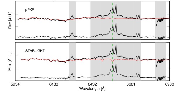
Figure 1: Example of stellar continuum modelling and its subtraction for NGC 4203 performed with different methods. The red line indicates the modelled stellar spectrum that matches the observed continuum, obtained applying the pPXF (top) and STARLIGHT (bottom) methods (Sect. 3.1). The most relevant spectral features blocked for modelling a line-free continuum are shown in gray. The rest frame H$\alpha$ wavelength is marked in green with dashed lines as reference. In this case, the output of STARLIGHT better reproduce the stellar continuum with respect to pPXF. This LINER shows complex H$\alpha$-[N II] emission-line profiles which are not studied in detail in this paper (see text).

Figure 2: Stellar continuum modelling obtained with pPXF (in red) for the template galaxy NGC 4026 (Sections 2 and 3.1) in both blue (top) and red (bottom) bandpasses. The spectral window excluded are shown in gray as in Fig. 1. The rest frame [O III]$\lambda$5007 and H$\alpha$ wavelength are marked in green with dashed lines as reference.

3 Analysis of the nuclear spectra

All the spectra have been shifted to rest-frame wavelengths using the values of the redshift provided by NED (Table 1).

3.1 Stellar Subtraction

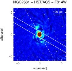
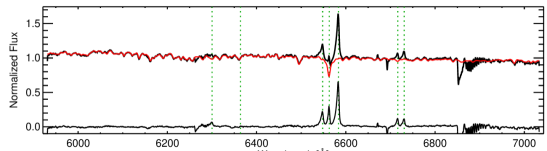
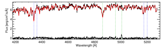
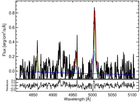
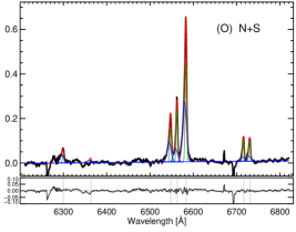
Figure 17: (General description as in Fig. 13.) NGC 2681: as in the case of NGC 0841, H$\alpha$ is strongly affected by stellar absorption in the observed spectrum. All emission lines are rather narrow, a dip is seen blueward of both [O I] and [S II]. After applying the procedure of the line modelling and by visual inspecting all the results (Sect. 3.2), the broad component appears to be absent. Contrary to HFS97, we did not find any tail (indicative of a broad component) in [N II] and the Fe I$\lambda$6523 feature is absent in our spectrum.

Reliable measurements of emission and absorption lines require a proper account of the starlight contamination. We applied a penalized PiXel fitting analysis (pPXF version 4.71; Cappellari & Emsellem 2004; Cappellari 2017) for the recovery of the shape of the stellar continuum. This underlying continuum spectrum is then subtracted to the one observed to obtain a purely interstellar medium (ISM) spectrum.
To produce a model of the stellar spectrum that matches the observed line-free continuum (any ISM features, atmospheric absorption and residuals from sky lines subtraction from data reduction were masked out), we used the Indo-U.S. stellar library (Valdes et al., 2004) as in Cazzoli et al. (2014, 2016). Briefly, this library is constituted of 1273 stars selected to provide a broad coverage of the atmospheric parameters (effective temperature T_eff, surface gravity log(g) and metallicity [Fe/H]) as well as spectral types. Nearly all the stellar spectra (885) have a spectral coverage from 3460 to 9464 Å, at a resolution of $\sim$ 1 Å FWHM (Valdes et al., 2004). Additionally, we set the default value for the bias parameter (see pag.144 in Cappellari & Emsellem 2004), and the keyword for linear regularization was fixed to zero. We also assumed a constant noise (i.e. the standard deviation calculated from a line-free continuum considering a wavelength range of either 20 or 60 Å) per pixel.
The stellar model subtraction leaves in few cases some residuals in the region blueward of [O I] (e.g. NGC 2681, Fig. 17). Despite this, the result of this approach is a model that in general reproduces the continuum shape well (the residuals are typically $<$ 10$\%$).
In order to check the robustness of the pPXF modelling for all the LINERs in the sample, we also modelled the stellar continuum with STARLIGHT V. 04 (Cid Fernandes et al., 2005, 2009), using single stellar populations from Bruzual & Charlot (2003). The spectra in this library have a spectral resolution of 3 Å guaranteeing enough spectral coverage to fit our data ($\sim$ 3200-9500 Å). Our templates include simple stellar populations of 25 different stellar ages (from 0.001 to 18 Gyr) and solar metallicity. We used the extinction law of Cardelli, Clayton & Mathis (1989), as in Pović et al. (2016). During the fits, any region with either ISM lines, or atmospheric absorption were ignored, as for the pPXF-modelling.
The reliability of the stellar model is difficult to evaluate considering the large wavelength coverage of our data ($\sim$ 1000-2000 Å) and the absence of unambiguous stellar absorption features (e.g. in the near-IR the CO$\lambda$$\lambda$2.293,2.322 bands). For example, the model might fit well the stellar continuum in the blue part of the spectra but not in the red one (e.g. NGC 2681, Fig. 12). Therefore, we visually inspected all the results from both pPXF and STARLIGHT fitting procedures noting that generally the pPXF model better reproduces the global continuum shape with lower residuals. In those few cases for which the pPXF modelling was not satisfactory, we selected the STARLIGHT output for the following analysis. Specifically, we adopted the STARLIGHT continuum model for blue and red spectra in one and six cases, respectively. In only one case (NGC 4036) we assumed the continuum model from STARLIGHT for both spectra. An example of the pPXF-STARLIGHT comparison is shown in Fig. 1; for all the other cases we refer to Fig. 12 of Appendix A.
Applying the pPXF fitting analysis also to our template galaxies (Sect. 2), in five cases (NGC 2950, NGC 3838, NGC 4026, NGC 4371, NGC 4382 and NGC 7332, Table 9) we found the presence of weak emission lines (mostly [O III]$\lambda$5007 and [N II]$\lambda$6584) in the residual spectra. An example is shown in Fig. 2, for the galaxy NGC 4026, for all the nine cases we refer to Fig. 11. The possible presence of ISM emission lines in the spectra of template galaxies may compromise the attainment of a final purely ISM-spectrum of LINERs. Hence, to account for this issue, we prefer the stellar subtraction obtained with either pPXF or STARLIGHT rather than using template galaxies.
For a more detailed discussion of different techniques for starlight subtraction we refer to Cappellari (2017).
The final selected procedure is listed for all the LINERs in Tab. LABEL:T_kin (column 3). The observed spectrum, its stellar continuum model and the final emission-line spectrum, are shown for each LINER in Appendix B.
We did not apply any procedure for the subtraction of the underlying stellar light for HST/STIS spectra as their limited wavelength coverage prevents an optimal stellar-continuum modelling. However, the contamination by the host-galaxy stellar continuum is expected to be small as the HST/STIS aperture is much smaller than those for ground-based observations (see Sect. 2 and Table 2). The results of the stellar continuum modelling of HST/STIS spectra by Shields et al. (2007), for four LINERs in common with our sample (NGC 2787, NGC 4143, NGC 4203 and NGC 4450), support that the stellar light contamination is small at HST/STIS scales.

3.2 Emission line fitting

After the subtraction of the stellar contribution (Sect. 3.1), each of the emission lines [O I]$\lambda$$\lambda$6300,6363, H$\alpha$$\lambda$6563, [N II]$\lambda$$\lambda$6548,6584 and [S II]$\lambda$$\lambda$6716,6731 in the spectra were modelled with single or multiple Gaussian-profiles with a Levenberg-Marquardt least-squares fitting routine (MPFITEXPR, implemented by Markwardt 2009) within the Interactive Data Analysis environment. We have imposed that the intensity ratios between the [N II]$\lambda$6548 and the [N II]$\lambda$6583 lines, and the [O I]$\lambda$6363 and the [O I]$\lambda$6300 lines satisfied the 1:3 and 1:2.96 relations, respectively (Osterbrock & Ferland, 2006). The fit was performed simultaneously for all lines using Gaussians and we consider one (or two) template(s) as reference for central wavelength(s) and line width(s) of the Gaussian curves. We did not use H$\alpha$ or [N II] as template since these lines are generally blended, and this may compromise the results of the fitting. Thus, each spectrum is fitted with three distinct models using [S II], [O I] or both, as reference.

S-model. The first model consists on modelling the [S II] lines and then tie all narrow lines to follow the same shifts and widths.
O-model. The second model is similar to the S-model but considering the [O I] lines as reference. This is particularly helpful as Oxygen lines are typically not-blended contrary to [S II].
M-model. The last model we tested is a ‘mixed’ line-modelling. It encompasses two possibilities with different assumptions. On the one hand, we considered that [S II] probes [N II], and [O I] traces the narrow H$\alpha$ (M1). On the other hand, we assumed that narrow H$\alpha$ and [N II] follow [O I] with [S II] line behaving otherwise (M2).

The use of [S II] or [O I] lines as template for modelling the H$\alpha$-[N II] is motivated by the stratification density in the narrow line region (NLR). Since a high difference in critical densities do exist for forbidden lines ions, $\sim$ 10³ cm^-3 for [S II], $\sim$ 10⁴ cm^-3 for [N II] and $\sim$ 10⁶ cm^-3 for [O I], the line profiles are expected not to be the same (see Balmaverde & Capetti 2014). Moreover, in the case of strong shocks being present in the ionised regions an enhanced [O I] emission is expected in relation to the other ions.
The procedure is aimed at obtaining the best-fitting to all emission lines and is organized in four steps as follows.
First, we tested all the models considering one Gaussian per each forbidden line and narrow H$\alpha$ (hereafter, narrow component). Second, after visual inspecting all the spectra and the results from the precedent step, for strongly asymmetric forbidden lines profiles, we tested a two-components line fitting. In these cases, the procedure adds a second Gaussian of intermediate width (hereafter, second component) following the three models listed above.
To prevent overfit models and allow for the appropriate number of Gaussians, we first calculated the standard deviation of a portion of the continuum free of both emission and absorption lines ($\varepsilon_{\rm c}$). Then we compare this value with the standard deviation estimated from the residuals under [S II] and [O I] obtained once the underlying stellar population has been substracted ($\varepsilon^{\rm line}$). We are quite conservative and have considered a reliable fit when $\varepsilon^{\rm line}$ $<$ 3 $\times$ $\varepsilon_{\rm c}$. Table LABEL:T_rms in Appendix A summarises all the $\varepsilon_{\rm c}$ and $\varepsilon^{\rm line}$ measurements.
Third, a broad H$\alpha$ component is added if needed to reduce significantly the residuals and the standard deviation when compared to single and double component(s) modelling. To assess whether the addition of a broad component is significant we estimated the $\varepsilon^{\rm line}$-level of confidence of our fitting as in the previous step (but in correspondence with H$\alpha$-[N II]) and adopting the same criterion to avoid overfitting.
Finally, we considered the best-fitting model for H$\alpha$ as template for H$\beta$$\lambda$4861, as these lines are expected to arise in the same region. Similarly, the [O III]$\lambda$$\lambda$4959,5007 emission lines are tied to follow the [S II] emission lines as they both originate in the NLR. Considering this the general behaviour, exceptions could be explained in terms of a more complex stratification in the ionization state and/or density of the gas in the NLR (being the critical density of [O III] of $\sim$ 10⁵ cm^-3). For this step of the procedure, we also imposed the intensity ratios between the [O III]$\lambda$4959 and the [O III]$\lambda$5007 satisfied the 1:2.96 relation (Osterbrock & Ferland, 2006). This last step of the procedure has been applied only to ground spectroscopic data as only the red HST/STIS bandpass is available (Sect. 2).
Overall, our fitting procedure includes three different physical models either with (M-models) or without (S- and O-models) stratification of the NLR. These models span four possible combinations of the components to reproduce the emission line profiles. Specifically, one or two components per forbidden line and narrow H$\alpha$, and each of these alternatives with an additional broad component in H$\alpha$.
A summary of the different models and combinations considering all the LINERs and data sets is given in Table 4. The adopted line modelling of the observed line profiles for both ground- and space-based spectroscopic data are shown in Figures from 13 to 34 of Appendix B; we also briefly describe the line profiles seen in ground-based data and their modelling (in the captions of the figures in Appendix B).
The selected best-fitting models are listed for each LINER in Tab. LABEL:T_kin, along with the velocity and velocity dispersion for each component. We corrected the observed line width $\sigma_{\rm line}$ for the effect of instrumental dispersion (Sections 2 and 2.1) by subtracting it in quadrature from the observed line dispersion ($\sigma_{\rm obs}$): $\sigma_{\rm line}$= $\sqrt{\sigma_{\rm obs}^{2}\,-\,\sigma_{\rm INS}^{2}}$.

3.2.1 Ground-based spectroscopy

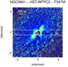
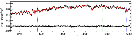
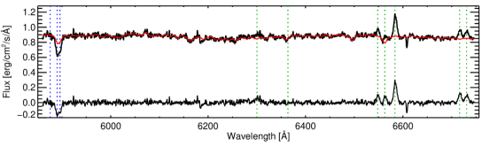
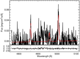
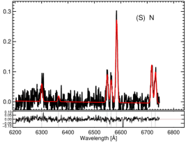
Figure 15: (General description as in Fig. 13.) NGC 0841: H$\alpha$ is strongly affected by stellar absorption in the observed spectrum (a good starlight subtraction is essential). All emission lines are well modelled with a single Gaussian component, no evidence for neither broad nor second components (H$\alpha$ and [N II] are well resolved). A visual inspection indicates that lines profiles are very different from those in the Palomar spectra (HFS97).

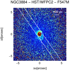
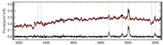
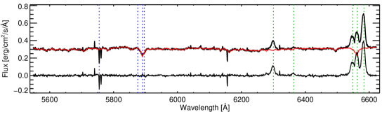
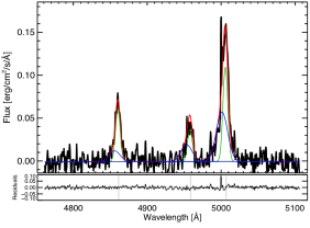
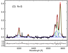
Figure 22: (General description as in Fig. 13.) NGC 3884: a blue wing is evident in the [O I] line. A broad component is not needed for the modelling of H$\alpha$. Tails and asymmetries are found by HFS97 when analyzing H$\alpha$-[N II] in the Palomar spectrum for this LINER but these are absent in our spectrum.

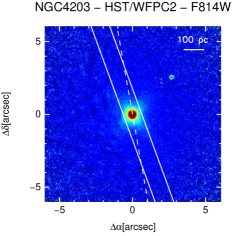
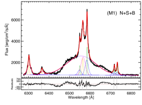
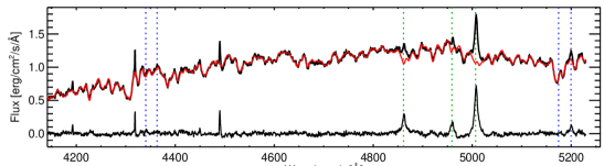
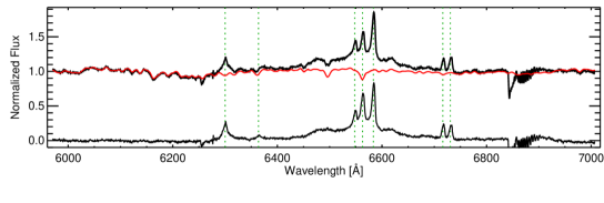
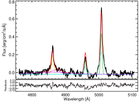
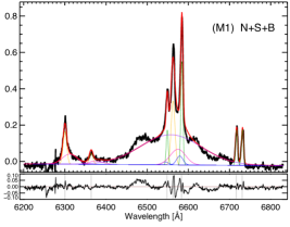
Figure 26: (General description as in Fig. 13.) NGC 4203: already a visual inspection indicates that H$\alpha$-[N II] lines seem quite different from those in the Palomar spectrum (HFS97). A red wing is evident in the [O I] profiles but not in [S II] lines which are contaminated by the broad H$\alpha$ component. A simple Gaussian fitting cannot reproduce well the line profiles due to the strong effect of the accretion disk in this galaxy (see text in Appendix B).

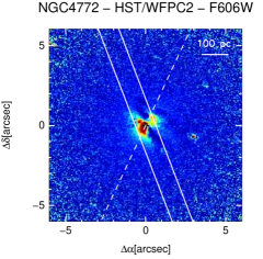
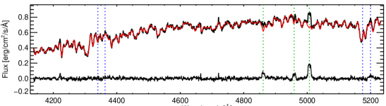
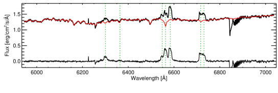
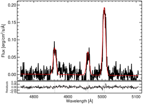
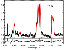
Figure 32: (General description as in Fig. 13.) NGC 4772: all emission line profiles are quite complex. The velocity curve is very chaotic with multiple kinematic components already in the individual spectra of the nuclear aperture we considered. In the extracted nuclear spectrum, the presence of a second component is evident for [O I] but not for [S II]. We tested a two-components fit for the forbidden lines, without obtaining a good modelling. We hence preferred to fit a single Gaussian for the narrow lines, though it results to be rather broad. Higher spectral resolution and S/N are needed to confirm the absence of any second and/or BLR components.

We tested the three models listed in Sect. 3.2 for our ground-based spectroscopic data. In two cases (NGC 0226 and NGC 3884) it was not possible to apply either S- or M-models as the wavelength coverage does not include [S II] lines (Sect. 2, Figures 13 and 22).
NGC 4203 represents an extreme case as three line components (narrow, second and broad) are not sufficient to reproduce well the H$\alpha$ line profile (Fig. 26). Its very broad and double-peaked emission line profile is likely originated in the outer parts of the accretion disc surrounding the SMBH (e.g. for a discussion of such model see Storchi-Bergmann et al. 2017). Thus, a more detailed modelling is needed (e.g. with a skewed Gaussian component as in Balmaverde & Capetti 2014) but this is beyond the aim of this work. Therefore, we excluded NGC 4203 from the analysis of ground-based data.
The use of a single Gaussian component for the forbidden lines and narrow H$\alpha$ provides already a good fit only in two cases: NGC 0841 and NGC 4772 (Table 4, Figures 15 and 32).
From our visual inspection, we note that [S II] and [O I] have strongly asymmetric profiles and their modelling requires two Gaussians (i.e. a single component fitting is an oversimplification) in many cases (i.e. 15/21 objects, Table 4). Therefore, in these cases, we applied a two-components line fitting to forbidden lines and narrow H$\alpha$. A two-Gaussians fit reproduces well the profiles of forbidden lines in all the 15 cases producing a final modelling accurate at $<$ 3 $\varepsilon^{\rm line}$ confidence (Table LABEL:T_rms).
In four cases (NGC 1052, NGC 3998, NGC 4438 and NGC 5005) the level of confidence calculated for H$\alpha$-[N II] is between 3.5 and 8 ($\varepsilon^{\rm line}$ in Table LABEL:T_rms). However, even if we tried to add the broad H$\alpha$ component in the modelling (step 3 in our procedure, Sect.3.2), the residuals were not lowered. Therefore, to avoid overfitting with a questionable Gaussian component we did not add the broad H$\alpha$ component.

Table 3: Results from the analysis of the optical spectra.

ID	Obs.	SF	Mod.	Comp.	VN${}^{\rm[S\,II]}$	$\sigma$N${}^{\rm[S\,II]}$	VN${}^{\rm[O\,I]}$	$\sigma$N${}^{\rm[O\,I]}$	VS${}^{\rm[S\,II]}$	$\sigma$S${}^{\rm[S\,II]}$	VS${}^{\rm[O\,I]}$	$\sigma$S${}^{\rm[O\,I]}$	VBHα	$\sigma$BHα
					km s-1	km s-1	km s-1	km s-1	km s-1	km s-1	km s-1	km s-1	km s-1	km s-1
NGC 0226	CAHA†	p/p	O	N + S	-	-	13 $\pm$ 2	165 $\pm$ 17	-	-	-296 $\pm$ 19	475 $\pm$ 50	-	-
NGC 0315	[NOT]	p/p	M1	N + S + B	-4 $\pm$ 6	88 $\pm$ 5	-24 $\pm$ 5	118 $\pm$ 31	-209 $\pm$ 148	485 $\pm$ 50	-288 $\pm$ 57	711 $\pm$ 144	374 $\pm$ 74	1051 $\pm$ 210
	HST †	-	S	N + S + B	54 $\pm$ 6	168 $\pm$ 8	-	-	-19 $\pm$ 4	397 $\pm$ 60	-	-	465 $\pm$ 70	1370 $\pm$ 165
NGC 0841	CAHA	p/p	S	N	31 $\pm$ 5	142 $\pm$ 10	(31 $\pm$ 5)	(142 $\pm$ 10)	-	-	-	-	-	-
NGC 1052	[NOT]	p/p	M2	N + S	-43  $\pm$ 2	121 $\pm$ 36	-123 $\pm$ 25	224 $\pm$ 49	11 $\pm$ 3	342 $\pm$ 71	-303 $\pm$ 16	761 $\pm$ 38	-	-
							-111 $\pm$ 10	265 $\pm$ 12			-340 $\pm$ 19	522 $\pm$ 78
	[HST]	-	M1	N + S + B	-104 $\pm$ 3	174 $\pm$ 9	-91 $\pm$ 2	186 $\pm$ 14	83 $\pm$ 17	331 $\pm$ 7	-66 $\pm$ 5	535 $\pm$ 5	12 $\pm$ 12	1238 $\pm$ 22
NGC 2681	CAHA	p/SL	O	N + S	(-41 $\pm$ 2)	(75 $\pm$ 26 )	-41 $\pm$ 2	75 $\pm$ 26	(-180 $\pm$ 8)	(209 $\pm$ 12)	-180 $\pm$ 8	209 $\pm$ 12	-	-
NGC 2787	CAHA	p/p	S	N + B	-5 $\pm$ 4	157 $\pm$ 13	(-5 $\pm$ 4)	(157 $\pm$ 13)	-	-	-	-	214 $\pm$ 67	542 $\pm$ 83
	HST ‡	-	S	N + B	110 $\pm$ 10	204 $\pm$ 6	(110 $\pm$ 10)	(204 $\pm$ 6)	-	-	-	-	228 $\pm$ 46	968 $\pm$ 32
NGC 3226	CAHA	p/p	O	N + S	(-58 $\pm$ 6)	(185 $\pm$ 20)	-58 $\pm$ 6	185 $\pm$ 20	(-155 $\pm$ 21)	(618 $\pm$ 45)	-155 $\pm$ 21	618 $\pm$ 45	-	-
NGC 3642	[CAHA]	p/p	M2	N + S + B	-33 $\pm$ 2	49 $\pm$ 25	-32 $\pm$ 6	70 $\pm$ 14	-49 $\pm$ 6	174 $\pm$ 7	-335 $\pm$ 67	300 $\pm$ 60	-228 $\pm$ 45	1341 $\pm$ 240
	[HST] †	-	S	N + B	71 $\pm$ 13	120 $\pm$ 21	-	-	-	-	-	-	191 $\pm$ 33	959 $\pm$ 81
NGC 3718	CAHA	p/p	M1	N + B	-110 $\pm$ 5	202 $\pm$ 13	-91 $\pm$ 7	261 $\pm$  7	-	-	-	-	-49 $\pm$ 10	1096 $\pm$ 219
NGC 3884	CAHA †	p/p	O	N + S	-	-	-64 $\pm$ 6	194 $\pm$ 10	-	-	-336 $\pm$ 32	456 $\pm$ 91	-	-
NGC 3998	[CAHA]	p/p	O	N + S	(-26 $\pm$ 2)	(203 $\pm$ 20)	-26 $\pm$ 2	203 $\pm$ 20	(-73 $\pm$ 15)	(713 $\pm$ 75)	-73 $\pm$ 15	713 $\pm$ 75	-	-
							-105 $\pm$ 7	196 $\pm$ 6			-228 $\pm$ 17	531 $\pm$ 21
	HST ‡	-	M1	N + B	194 $\pm$ 18	272 $\pm$ 4	202 $\pm$ 10	474 $\pm$ 5	-	-	-	-	0 $\pm$ 1	1870 $\pm$ 36
NGC 4036	CAHA	SL/SL	M1	N + S	6 $\pm$ 3	165 $\pm$ 10	-5 $\pm$ 3	85 $\pm$ 10	48 $\pm$ 5	379 $\pm$ 7	35 $\pm$ 12	332 $\pm$ 32	-	-
	HST	-	M1	N + B	240 $\pm$ 5	201 $\pm$ 13	242 $\pm$ 12	180 $\pm$ 4	-	-	-	-	191 $\pm$ 38	1051 $\pm$ 210
NGC 4143	CAHA	p/SL	M2	N + S	46 $\pm$ 4	122 $\pm$ 9	32 $\pm$ 3	100 $\pm$ 10	-30 $\pm$ 6	222 $\pm$ 44	-15 $\pm$ 3	570 $\pm$ 22	-	-
	HST ‡	-	S	N + S + B	145 $\pm$ 9	168 $\pm$ 36	(145 $\pm$ 9)	(168 $\pm$ 36)	6 $\pm$ 2	320 $\pm$ 65	(6 $\pm$ 2 )	(320 $\pm$ 65)	540 $\pm$ 42	1492 $\pm$ 59
NGC 4203	CAHA	p/SL	M1	N + S + B	37:	110:	-4:	210:	-197:	356:	545:	846:	-251:	3494:
					53:	141:			104:	368:
	[HST]	-	M1	N + S + B	102:	68:	82:	111:	20:	369:	163:	474:	-285:	3191:
NGC 4278	CAHA	p/p	M2	N + S	6 $\pm$ 7	177 $\pm$ 35	21 $\pm$ 2	180 $\pm$ 14	77 $\pm$ 34	240 $\pm$ 4	14 $\pm$ 46	669 $\pm$ 67	-	-
	HST ‡	-	M1	N + S + B	105 $\pm$ 12	172 $\pm$ 3	96 $\pm$ 27	189 $\pm$ 2	122 $\pm$ 106	536 $\pm$ 2	69 $\pm$ 28	737 $\pm$ 2	165 $\pm$ 32	1142 $\pm$ 228
NGC 4438	[CAHA]	p/p	M1	N + S	-50 $\pm$ 2	87 $\pm$ 22	-62 $\pm$ 2	68 $\pm$ 30	-5 $\pm$ 5	203 $\pm$ 10	35 $\pm$ 10	213 $\pm$ 42	-	-
NGC 4450	CAHA	p/p	M2	N + S	-17 $\pm$ 8	101 $\pm$ 6	-6 $\pm$ 4	133 $\pm$ 10	-15 $\pm$ 2	220 $\pm$ 30	-94 $\pm$ 15	451 $\pm$ 45	-	-
	HST	-	M1	N + S + B	108 $\pm$ 2	117 $\pm$ 13	109 $\pm$ 10	113 $\pm$ 3	-75 $\pm$ 43	442 $\pm$ 89	88 $\pm$ 19	442 $\pm$ 2	-89 $\pm$ 28	3125 $\pm$ 34
NGC 4636	CAHA	p/SL	S	N + B	165 $\pm$ 7	154 $\pm$ 8	(165 $\pm$ 7)	(154 $\pm$ 8)	-	-	-	-	-44 $\pm$ 97	914 $\pm$ 182
NGC 4750	CAHA	SL/p	O	N + S + B	(-32 $\pm$ 5)	(172 $\pm$ 28)	-32 $\pm$ 5	172 $\pm$ 28	(-296 $\pm$ 21)	(380 $\pm$ 42)	-296 $\pm$ 21	380 $\pm$ 42	328 $\pm$ 42	1005 $\pm$ 45
NGC 4772	CAHA	p/p	S	N	-21 $\pm$ 5	249 $\pm$ 12	(-21 $\pm$ 5)	(249 $\pm$ 12)	-	-	-	-	-	-
NGC 5005	[CAHA]	p/SL	S	N + S	92 $\pm$ 18	237 $\pm$ 47	(92 $\pm$ 18)	(237 $\pm$ 47)	-108 $\pm$ 22	446 $\pm$ 90	(-108 $\pm$ 22)	(446 $\pm$ 90)	-	-
	HST †	-	S	N + S + B	-96 $\pm$ 12	98 $\pm$ 20	-	-	-111 $\pm$ 22	302 $\pm$ 62	-	-	145 $\pm$ 29	914 $\pm$ 135
NGC 5077	CAHA	p/SL	S	N + B	-14 $\pm$ 4	195 $\pm$ 18	(-14 $\pm$ 4)	(195 $\pm$ 18)	-	-	-	-	168 $\pm$ 34	1188 $\pm$ 238
	HST †	-	S	N + S + B	93 $\pm$ 14	282 $\pm$ 16	-	-	-184 $\pm$ 37	397 $\pm$ 80	-	-	419 $\pm$ 80	1142 $\pm$ 170

Notes. ‘ID’: object designation as in Table 1. ‘OBS’: origin of the optical data. ‘Stellar fit’: assumed model for the stellar continuum in the blue and red spectra, ‘p’ and ‘SL’ stand for pPXF and STARLIGHT method, respectively. ‘Mod.’: best-fitting model for emission lines. ‘S’, ‘O’ and ‘M’ stand for models based on [S II] or [O I] or the two mixed-types (see text). ‘Comp.’: components used to achieve the best-fitting model. ‘N’, ‘S’ and ‘B’ stand for narrow, second and broad components, respectively. The velocity (‘V’) and velocity dispersion (‘$\sigma$’), for each component listed in column 5 and for the set of emission lines: [S II], [O I] and H$\alpha$. For three LINERs we cannot constrain H$\beta$ and [O III] using the results obtained for the red spectrum. Hence, we report V and $\sigma$ of these emission lines in a different line. Symbols indicate:
$(\ )$ the values obtained for those cases for which the shift and width of emission lines has been constrained using a different forbidden template (e.g. [S II] values when the O-model is adopted);
$[\ ]$ the data for which the fit of the H$\alpha$-[N II] emission is not constrained well;
^† the observed spectrum lacks either [S II] or [O I] preventing to test all the proposed fitting model;
^‡ the [O I] lines are at the edge of HST/STIS spectra;
: the measurements which are only indicative owed the need of a more elaborate physical modelling (NGC 4203).

Table 4: Summary of the models and components used to model emission lines.

		GROUND					SPACE
		[S II]	[O I]	M1	M2		[S II]	M1
Narrow		NGC 0841
		NGC 4772
Narrow + Second		[NGC 5005]
			NGC 0266 †
			NGC 2681
			NGC 3226
			NGC 3884 †
			[NGC 3998]
					[NGC 1052]
				NGC 4036
					NGC 4143
					NGC 4278
				[NGC 4438]
					NGC 4450
Narrow + Second + BroadHα			NGC 4750
				[NGC 0315]
					[NGC 3642]
								[NGC 1052]
							NGC 0315 †
							NGC 4143 ‡
							NGC 5005 †
							NGC 5077 †
								NGC 4278 ‡
								NGC 4450
Narrow + BroadHα		NGC 2787
		NGC 4636
		NGC 5077
				NGC 3718
							NGC 2787 ‡
							[NGC 3642] †
								NGC 3998 ‡
								NGC 4036

Notes. Rows display the four possible combinations of the components to reproduce the emission line profiles (Sect. 3.2). Columns indicate the different physical models (Sect. 3.2) considered for both ground- and space-based data as indicated on the top. The object designation is as in Table 1. ^† and ^‡ symbols and square-brackets are the same of Table LABEL:T_kin.

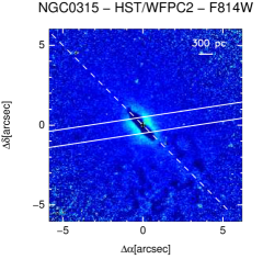
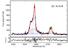
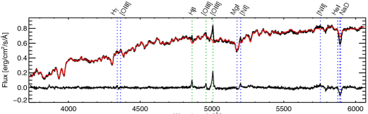
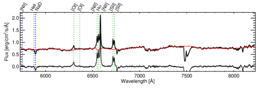
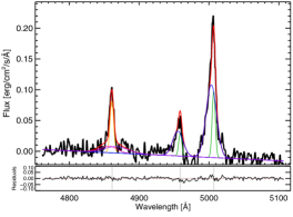
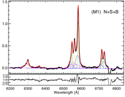
Figure 14: (General description as in Fig. 13.) NGC 0315: [O I] lines are asymmetric and the [S II] doublet is rather broad. These considerations suggest the presence of two different second components both blueshifted but with different widths. We did not find a clear improvement of the standard deviation in H$\alpha$ for the ground-based data fitting when adding the broad component (Table LABEL:T_rms). However, the presence of a red wing near the base of [N II]$\lambda$6584 (absent in the other template lines) makes the broad component necessary to adequately model the H$\alpha$-[N II] complex. Thus a broad component is needed for a good fit, but its presence is not obvious and it is rather weak (in good agreement with HFS97).

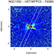
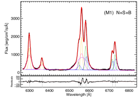
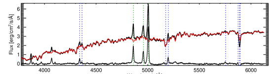
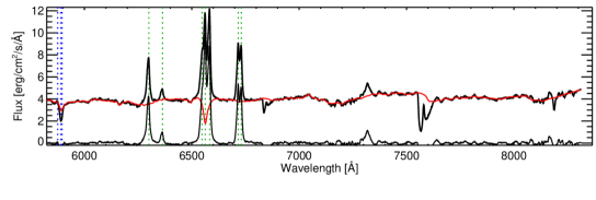
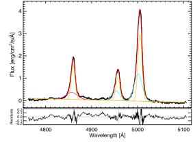
Figure 16: (General description as in Fig. 13.) NGC 1052: broad blue wings are evident in [O I] but not in [S II]. The second component in [O III] (light blue curves) seems to behave otherwise compared to all the other emission lines. We also report the detection of [Ca II]$\lambda$$\lambda$7291,7324 and [O II]$\lambda$$\lambda$7318,7319,7330,7331 emission lines which are strongly blended.

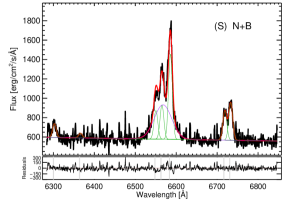
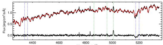
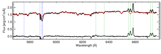
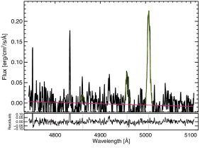
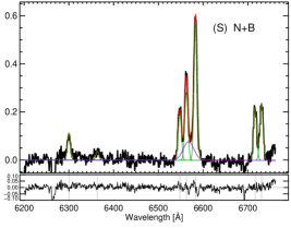
Figure 18: (General description as in Fig. 13.) NGC 2787: the H$\alpha$-[N II] line profiles are quite different from those in the Palomar spectra (HFS97). Specifically, there are not any indications of an extended red wing. Narrow lines are well modelled with one component, an additional broad H$\alpha$ component (which is fairly prominent, as for the Palomar spectrum) is needed to well reproduce the line profiles in our red spectrum. The S/N of the blue spectrum is low and H$\beta$ is very weak, what hamper the detection of an eventual broad H$\beta$ component.

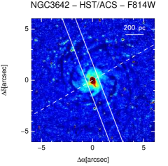
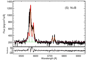
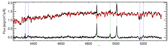
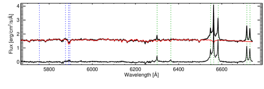
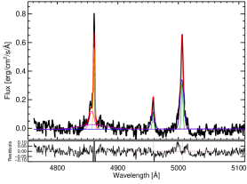
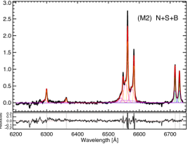
Figure 20: (General description as in Fig. 13.) NGC 3642: narrow emission lines have small widths and broad wings as found for the Palomar spectrum (HFS97). A small improvement of $\varepsilon$${}^{\rm[O\,I]}$ (0.0036, Table LABEL:T_rms) is found when using two components instead of one. The presence of wings in all emission lines suggests that the second component is true and not an artifact. The broad component is present but is relatively weak. We did not find difference in H$\alpha$ and [N II] line profiles contrary to the modelling proposed by HFS97. [O III]$\lambda$5007 seems to require a broader second component, but it is not clear for [O III]$\lambda$4959.

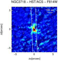
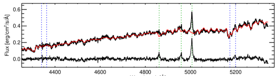
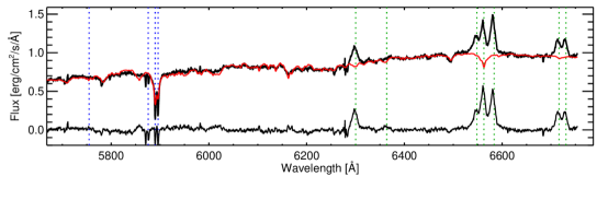
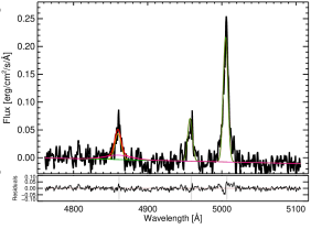
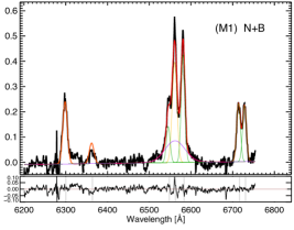
Figure 21: (General description as in Fig. 13.) NGC 3718: even if both [O I] and [S II] regions have some problems (i.e. dips, edge of the wavelength range) and H$\alpha$ and [N II] are strongly blended, the resulting fit is still satisfactory (Table LABEL:T_rms).

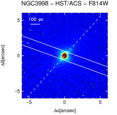
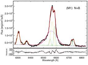
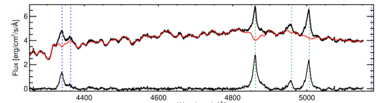
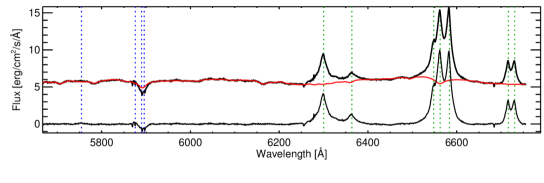
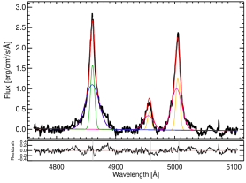
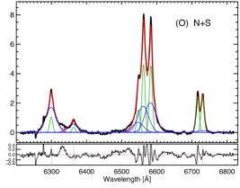
Figure 23: (General description as in Fig. 13.) NGC 3998: a second component is evident in the [O I] line being rather weak in [S II]. Issues related to the stellar subtraction might be at the origin of the small bump between Oxygen lines. The [O III] lines have different kinematics (light and pink curves) with respect to the other lines.

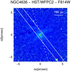
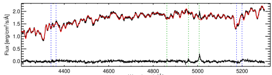
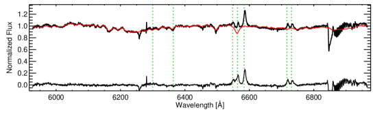
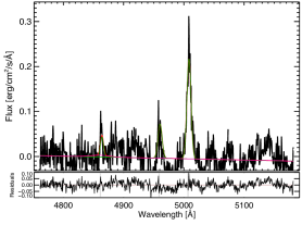
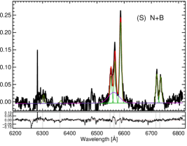
Figure 30: (General description as in Fig. 13.) NGC 4636: [O I] lines are very weak even after starlight subtraction. [S II] is therefore more reliable as a reference for modelling the narrow lines.

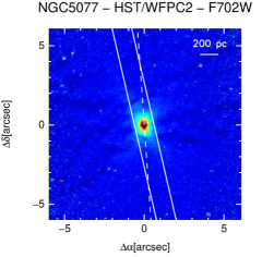
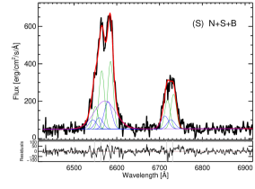
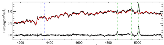
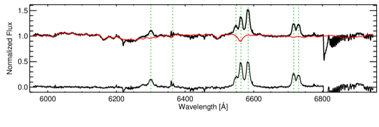
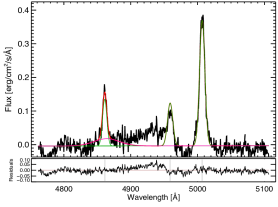
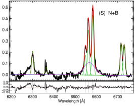
Figure 34: (General description as in Fig. 13.) NGC 5077: the [S II] profile is well fitted with one component, but [O I] seems to have a strong, broad and blueshifted wing. A broad H$\alpha$ component is necessary for a satisfactory fit. It is worth to note that the modelling proposed by HFS97 (which includes the broad component) depends on [S II] assumptions.

The addition of a broad H$\alpha$ component reduces significantly the residuals from the two-components fitting in four cases (3/15, NGC 0315, NGC 3642 and NGC 5750). Among these, in two cases (NGC 0315 and NGC 3642), the modelling is accurate to $\sim$ 4-5 ($\varepsilon^{\rm line}$ in Table LABEL:T_rms; Figures 14 and 20).
In four cases, namely NGC 2787, NGC 3718, NGC 4636 and NGC 5077, the forbidden lines do not require any second component, but H$\alpha$ is clearly broad and the BLR component is essential for an adequate fitting (Figures 18, 21, 30 and 34).
In the peculiar case of NGC 1052 (Fig. 16) to obtain a good fit we displace the second Gaussian needed to model [O III] lines with a shift larger then the uncertainties estimated when modelling [S II]. In the exceptional case of NGC 3998 (Fig. 23), we also shifted the narrow component of [O III].

3.2.2 Space spectroscopy

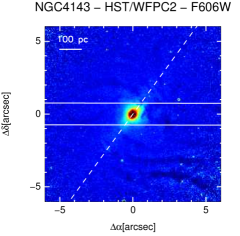
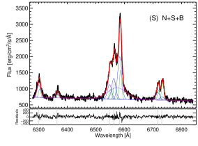
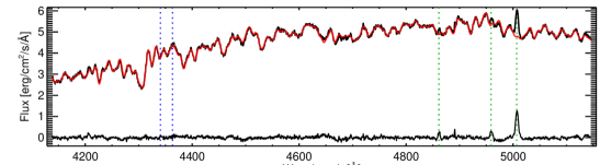
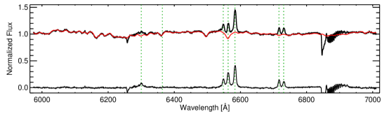
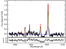
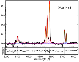
Figure 25: (General description as in Fig. 13.) NGC 4143: [S II] and [O I] line profiles are quite different with the latter having more pronounced wings. Similarly to the case of NGC 2682, redward to [O I] there is a dip. H$\beta$ is rather weak and symmetric. HFS97 assumed [S II] as template while we considered [O I], this may be at the origin of the contradictory results concerning the broad H$\alpha$ component (Table LABEL:T_FWHM).

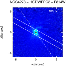
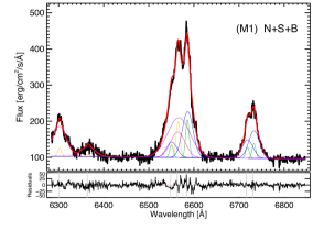
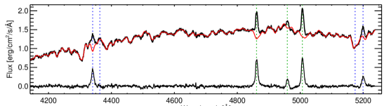
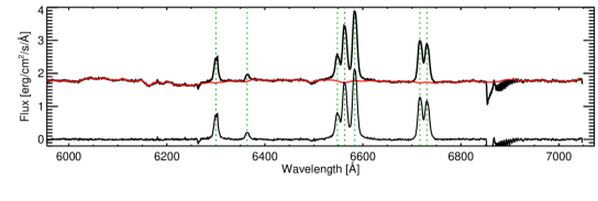
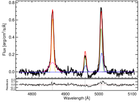
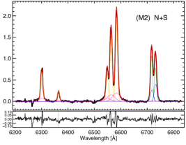
Figure 27: (General description as in Fig. 13.) NGC 4278: the stellar H$\alpha$ absorption seems to be negligible. We did not find evidence for a broad component in our ground-based spectra, whereas it is relatively weak in the Palomar spectrum (HFS97).

We applied the same procedure described in Sect. 3.2 for modelling the observed emission line profiles in HST/STIS spectroscopic data (Sect. 2.1) for the 12 LINERs in common with Balmaverde & Capetti (2014). As for ground-based spectroscopy, we exclude NGC 4203. This LINER is an extreme case (Sect. 3.2.1) whose detailed modelling is beyond the aim of this work.
We attempted to test the three models for the remaining 11 LINERs except for four cases, namely NGC 0315, NGC 3642, NGC 5005 and NGC 5077. For these objects it was not possible to apply either O- or M-models since the wavelength coverage of our HST/STIS does not include the [O I] lines. This is a strong limitation in the case of NGC 3642, as we were not able to obtain a satisfactory fit using only [S II] as reference, since these lines are rather weak (Fig. 20).
For four LINERs (namely, NGC 2787, NGC 3998, NGC 4143 and NGC 4278), the line modelling of [O I] is complicated by the fact that these forbidden lines are observed at the edge of the HST/STIS spectra (Figures 18, 23, 25 and 27). This hinders a robust estimate of the line shifts and widths of any second component (generally identified as a wing of the line profiles).
Overall, in four (seven) cases is adequate one (two) Gaussian(s) per reference forbidden line and narrow H$\alpha$. In all 11 cases, a broad H$\alpha$ BLR-originated component is required (Table LABEL:T_kin). In all 11 cases, the modelling of forbidden lines is accurate at $<$ 3 $\varepsilon^{\rm line}$ level. However, this is not the case for the H$\alpha$-[N II] complex since in two cases (2/11, NGC 1052 and NGC N3642) the level of confidence is $\varepsilon^{\rm line}$ $\sim$ 5-6.

3.3 Absorption line fitting in ground-based data

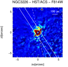
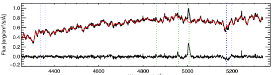
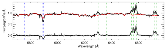
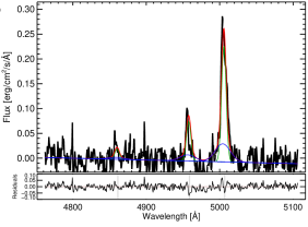
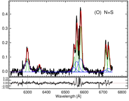
Figure 19: (General description as in Fig. 13.) NGC 3226: in spite of the [S II] lines being at the red end of the spectrum, a satisfactory line fitting is reached. Even if a single-component model of [O I] produces lower residuals than the double Gaussians one, its resulting width ($\sim$ 500 km s^-1) is unrealistically large, what made us conclude that a two-components models is better in this case.

In 11 out of 22 of the LINERs in the sample, the wavelength coverage of our ground spectroscopic data allows to probe the NaD$\lambda$$\lambda$5890,5896 absorption lines (see figures in Appendix B). Such a spectral feature originates both in the cold-neutral ISM of galaxies and in the atmospheres of old stars (e.g. K-type giants, Jacoby, Hunter & Christian 1984). The residual spectrum (after the stellar subtraction, Sect. 3.1) grants the study of the cold neutral gas in LINERs based on a purely-ISM NaD feature. Hence, the study of the NaD ISM-absorption allows us to infer whether the cold neutral gas is either participating to the ordinary disc-rotation or entraining in a multiphase outflow. These two possible scenarios have different impacts on the host-galaxy evolution (e.g. Cazzoli et al. 2016).
In the case of NGC 3718 (Fig. 21), the spectral region from 5860 to 5910 Å  is dominated by telluric absorption, preventing any putative detection of the NaD doublet. In two cases (NGC 3642 and NGC 3884, Figures 20 and 22) the ISM-NaD seems to be present as a weak resonant NaD emission that may indicate the presence of dusty outflows (see Rupke & Veilleux 2015). However, in these two cases, data at higher S/N are needed to confirm such an unfrequent detection. We then excluded for the line modelling and the following analysis these three cases as the NaD detection is highly uncertain.
In the remaining eight cases (namely NGC 0266, NGC 0315, NGC 0841, NGC 1052, NGC 2787, NGC 3226, NGC 3998 and NGC 4750) the subtraction of a purely-stellar NaD feature leaves a strong residual, suggesting that its origin is mainly interstellar. In three cases (NGC 2787, NGC 3226 and NGC 3998), the purely ISM-originated NaD is either weak and/or affected by sky/telluric lines especially evident blueward of the doublet (see Figures 18, 19 and 23).
As for emission lines (Sect. 3.2), the ISM-NaD absorption was modelled with Gaussians. We first considered two Gaussian profiles i.e. a single kinematic component (as in Davis et al. 2012, Cazzoli et al. 2014 and Cazzoli et al. 2016). Specifically, the central wavelength of the NaD$\lambda$5890 is a free parameter, while the widths are constrained to be equal for the two lines. In addition, the ratio between the equivalent widths (EW) of the two lines, R_NaD = EW₅₈₉₀/EW₅₈₉₆, is restricted to vary from 1 (i.e. optically thick limit) to 2 (i.e. optically thin absorbing gas) according to Spitzer (1978). This fitting method allows to infer global neutral gas kinematics as with our data we are not able to map and constrain individual gas clouds motions (i.e. many subcomponents) eventually present along the line of sight. For a more detailed discussion of the limitations of the method we refer to Rupke, Veilleux & Sanders (2005a) and Cazzoli et al. (2016).
In the procedure for modelling the NaD absorption, we did not take into account the He I$\lambda$5876 line (as done in some previous works e.g. Cazzoli et al. 2016) since it is generally not observed in these objects. The only two exceptions are the rather weak He I detections in NGC 0315 and NGC 1052 (Figures 14 and 16).
In general, the modelling of the NaD line profile is rather complicated and sometimes leads to unphysical or non-unique solutions. Therefore, in order to preserve against spurious results, as an initial guess, the Gaussian components were constrained to have the same velocity shift and line width of H$\alpha$, testing both narrow and second (if present) components (similarly to Cazzoli et al. 2014). From this initial guess, we tried to obtain the best-fitting to the NaD absorption preventing overfitting.
For all cases, we tested a two-component modelling by adding a second broader kinematic component to the one Gaussian-pair fit (similarly to the procedure described in Sect. 3.2), but the majority of the spectra have not strongly asymmetric profiles and their modelling requires only one component. Only in the case of NGC 0266, we find that a two-Gaussian components model per doublet led to a remarkably good fit of the NaD absorption, also reducing the residuals (especially in the wings of the absorption profile) with respect to one-Gaussian fits (from $\sim$2 $\varepsilon^{\rm line}$ to 1.3 $\varepsilon^{\rm line}$ confidence level). In this case, the broadest component is called ‘second component’ (similarly to emission lines).
The line modelling of the NaD profiles in ground-based spectroscopic data are shown in Fig. 3. The line properties (shift and width) and line ratios (R_NaD) for each component are reported in Table 5.

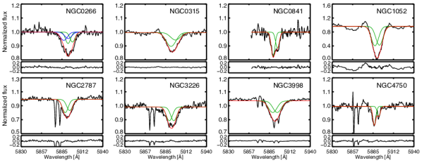
Figure 3: Normalized spectra of the NaD absorption-line profile after the subtraction of the stellar contribution, for those LINERs having robust detection of the doublet (see Sect. 3.3). Each displayed spectrum covers a rest-frame range of $\sim$ 110 Å  (i.e. $\sim$ 5500 km s^-1). The different kinematic components are shown in green and blue, i.e. narrow and second component, according to our classification (see Sect. 3.2). The red curve shows the total contribution coming from the NaD Gaussian fit. In the lower panels, the residuals (i.e. data - model) are presented.

4 Main observational results

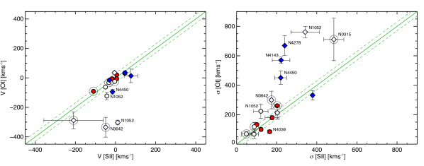
Figure 5: Comparison between the velocity (left) and velocity dispersion (right) values for the different components in M-models (both M1 and M2). Red circles and blue diamonds indicate narrow and second components. Empty symbols indicate that the corresponding H$\alpha$ measurement is less reliable (TableLABEL:T_rms and Sect. 3.2.1). An additional circle marks those cases for which a broad component is needed to improve the fit. The green continuos line marks the 1:1 relation. The green dashed lines represents the positions for which the velocity (velocity dispersion) of [S II] is equal to $\pm$ 30 km s^-1 that of the [O I]. The total range of 60 km s^-1 roughly corresponds to the instrumental dispersion of our ground-based TWIN/CAHA data (Sect. 2). The IDs of outliers are also indicated (see text for details).

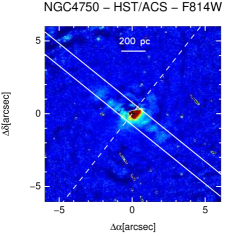
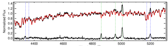
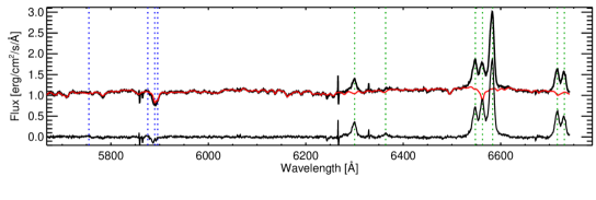
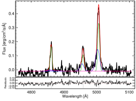
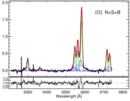
Figure 31: (General description as in Fig. 13.) NGC 4750: some residuals from the sky subtraction affect the region of [O I] and that of [S II] is at the edge of the spectrum. In spite of this, we were able to obtain a good fit for the forbidden lines with two components. We did not find a clear improvement of the standard deviation in H$\alpha$ for the ground-based data fitting when adding the broad component (Table LABEL:T_rms). However, the presence of a red wing near the base of [N II]$\lambda$6584 (absent in the other template lines) makes the broad component necessary to adequately model the H$\alpha$-[N II] complex. Thus a broad component is needed for a good fit, but its presence is not obvious and it is rather weak (in rather good agreement with HFS97).

For ground-based data, the S-model and O-model reproduce well the line profiles in six of the cases each, while a larger fraction of cases (i.e. 9/21) require M-models (4 and 5 cases for M1 and M2, respectively) for a satisfactory fit (Table LABEL:T_kin).
Of the four possible combinations of components listed in Sect. 3.2 (see also rows in Table 4), one Gaussian per forbidden line (with width lower than 250 km s^-1) is adequate in 6 out of 21 cases. More specifically, we found that only in two cases (NGC 0841 and NGC 4772, Figures 15 and 32), one Gaussian reproduce well all emission lines including H$\alpha$ (the broad component is not required). A broad Gaussian for H$\alpha$ is required in the remaining four cases (see Table 4).
In the large majority of the cases (15/21), two Gaussians per forbidden line are required for a satisfactory modelling (Tables LABEL:T_kin and Table 4). Among this 15 cases, only in three cases (NGC 0315, NGC 3642 and NGC 4750, Figures 14, 20 and 31) an additional broad H$\alpha$ component is required to reproduce well the observed line profiles (i.e. for a total of three kinematic components). For the remaining 12 cases the broad component is not required (Table 4). For this subsample of 15 LINERs, there are only six cases (Table 4) for which the presence/absence of the BLR-component is less reliable in terms of $\varepsilon^{\rm line}$-uncertainty (Sect. 3.2.1 and Table LABEL:T_rms).
Overall we required the broad H$\alpha$ component in 7 out of 21 cases.
Table LABEL:T_sum_kin summarises the mean(median) value(s) for the velocity (V), velocity dispersion ($\sigma$) and FWHM of the different components for each data set, as well as the standard deviation for the distribution of our measurements.
In Fig. 4, we show the comparison between the velocity and velocity dispersion of the narrow and second components used to fit emission lines for each of the proposed models. Velocities of the narrow components are close to rest frame (on average V = -10 km s^-1, Table LABEL:T_sum_kin), varying between $\pm$ 110 km s^-1 (Table LABEL:T_kin). There are two exceptions: NGC 1052 (whose fitting is less reliable, Table LABEL:T_rms, Fig. 16) and NGC 4636 (Fig. 30) having [O I] velocities of $\sim$ -125 km s^-1 and $\sim$ 165 km s^-1, respectively. The velocity dispersion value for the narrow components is $\sigma$ = 157 km s^-1, on average (Table LABEL:T_sum_kin). For the second components the velocity range is larger varying from -350 km s^-1 to 100 km s^-1. The velocity dispersion varies between 150 and 800 km s^-1 being generally broader (on average $\sigma$ = 429 km s^-1, Table LABEL:T_sum_kin) than those of narrow components.
Fig. 5 shows the comparison between the velocity and velocity dispersion of the narrow and second components used to fit [O I] and [S II] emission lines for the nine LINERs for which we adopt M-models to fit emission lines (Table 4).

Table 5: Table that summarises all the results from NaD absorption.

ID	VNaD	$\sigma$NaD	RNaD
	km s-1	km s-1
NGC 0266	165 $\pm$ 33	171 $\pm$ 34	1.2
	-125 $\pm$ 25	238 $\pm$ 48	1.3
NGC 0315	117 $\pm$ 48	335 $\pm$ 67	1.9
NGC 0841	2 $\pm$ 2	126 $\pm$ 23	1.5
NGC 1052	-122 $\pm$ 24	245 $\pm$ 49	1.0
NGC 2787	-28 $\pm$ 6	202 $\pm$ 40	1.2
NGC 3226	2 $\pm$ 2	212 $\pm$ 42	1.0
NGC 3998	-18 $\pm$ 4	292 $\pm$ 58	1.0
NGC 4750	-163 $\pm$ 33	104 $\pm$ 21	1.9

Notes. ‘ID’: object designation as in Table 1. Velocity (‘V_NaD’) and velocity dispersion (‘$\sigma$_NaD’) of the neutral gas. As the fit was rather complicated leading to spurious solutions, we conservatively quoted the 20$\%$ uncertainty. The NaD doublet in NGC 0266, has been modelled with two kinematic components whose values are reported in a different line. ‘R_NaD’  indicates the ratio between the EWs of the two lines of NaD (Sect. 3.3).

If we consider the individual narrow components (red circles in Fig. 5) in M-models (both M1 and M2), we found a general agreement within a tolerance of $\pm$ 30 km s^-1 (globally of the order of the instrumental dispersion of CAHA/TWIN data, i.e. $\sim$ 60 km s^-1, Sect. 2) between the velocity and velocity dispersion of narrow-[O I] and narrow-[S II]. The only exception in velocity dispersion is NGC 4036 (Fig. 5; Table LABEL:T_kin). Two exceptions (NGC 3642 and NGC 4450) are found for the velocities of the secondary component (diamonds in Fig. 5). However, of these two cases only NGC 4450 should be considered a true outlier: as the fit of the H$\alpha$-[N II] complex is less reliable (Table LABEL:T_rms) for NGC 3642. We found less agreement when comparing velocity dispersion values for the second component, with [O I] lines profiles being typically much broader than [S II]. The difference is up to a factor of $\sim$ 3 in the case of NGC 4278 (Fig. 5 right; Table LABEL:T_kin).
In these comparisons, taking into account the (larger) instrumental dispersion of NOT/ALFOSC data, NGC 1052 should not considered as outlier neither in velocity or in velocity dispersion.
A broad H$\alpha$ component (FWHM $>$ 1200 km s^-1) is required only in 7 out of 21 of the LINERs (i.e. 33$\%$, Table LABEL:T_kin). The BLR component is found mainly when we adopt S- and M-models (three cases each, Table LABEL:T_sum_kin), with the latter modelling giving less reliable measurements in two cases (NGC 0315 and NGC 3642, Table LABEL:T_rms).
The measured FWHM of the broad component ranges from 1277 km s^-1 (NGC 2787) to 3158 km s^-1 (NGC 3642); the average value is 2401 km s^-1 (Table LABEL:T_sum_kin). The velocity varies from -228 (NGC 3642) to 374 km s^-1 (NGC 0315) though both from less reliable measurements; otherwise, excluding those less reliable values, the velocity range would be $\sim$ -50 to $\sim$ 330 km s^-1 (Table LABEL:T_kin).
For none of the 11 HST/STIS spectra, the adopted best fit is obtained using the O-model. Excluding those four cases for which we were not able to test all the proposed models (Sect. 3.2.2, Table LABEL:T_kin), we found a slightly large prevalence of best fits obtained with M-models, i.e. 5/7 (Table 4). For all these five cases we adopted the M1-model.
In four cases (NGC 2787, NGC 3642, NGC 4036 and NGC 3998), one Gaussian per forbidden line and narrow H$\alpha$ (typically with $\sigma$ between 120 and 270 km s^-1, Table LABEL:T_kin) is adequate. In the remaining cases, two Gaussians are required for a good fit of forbidden lines, due to the presence of broad wings in the line profiles.
The broad component in HST/STIS spectra is ubiquitous (Table 4).

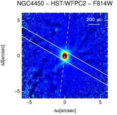
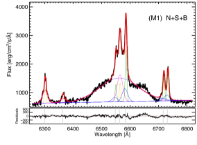
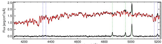
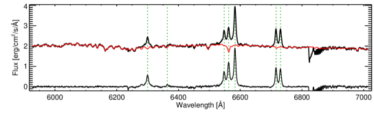
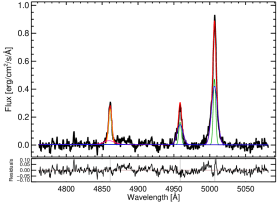
Figure 29: (General description as in Fig. 13.) NGC 4450. Forbidden lines are rather broad even before the stellar subtraction. [O I] ([S II]) line-profiles have blue (red) wings.

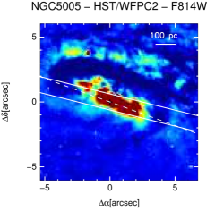
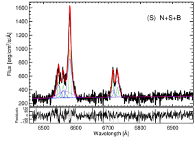
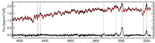
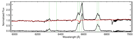
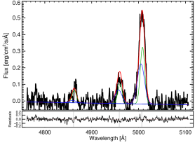
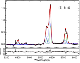
Figure 33: (General description as in Fig. 13.) NGC 5005: both H$\alpha$-[N II] and [S II] lines are strongly blended. We carefully tested all models (Sect. 3.2), and finally selected that based on [S II]. Even if a single-component model of [O I] produces lower residuals than the double Gaussians one, its resulting width is unrealistically large, what made us conclude that a two-component model is better in this case.

Except for a few cases (see columns 6-9 in Table LABEL:T_kin), narrow components have velocities between -100 and 200 km s^-1. The velocity dispersion is 176 km s^-1, on average (Table LABEL:T_sum_kin). Similarly, the velocities of second component range from -200 to 150 km s^-1. These second components are however broader, with velocity dispersion values between 300 and 750 km s^-1 (Table LABEL:T_kin); the average value is 433 km s^-1 (Table LABEL:T_sum_kin). If we consider the individual narrow components in M-models, we found a trend similar to that obtained considering the same model but with ground-based spectroscopy. Specifically, for the velocity and velocity dispersion of narrow components we found a general agreement with the same range of tolerance ($\pm$ 30 km s^-1, globally of the order of the instrumental dispersion of HST/STIS data, Sect. 2.1) considered in the spectral analysis of ground-based data (except NGC 3398, Table LABEL:T_kin). Less agreement is found for the velocity and velocity dispersions of the second components.
The measured FWHM of the broad H$\alpha$ components in HST spectra range from 2152 km s^-1 (NGC 5005, Fig. 33) to 7359 km s^-1 (NGC 4450, Fig. 29), with an average value of 3270 km s^-1 (Table LABEL:T_sum_kin).
For the NaD absorption, in 7 out of 8 targets, a single kinematic component (a Gaussian pair) already gives a good fit, suggesting that if a second component exists in these galaxies, it is weak. The only exception is NGC 0266, which requires two Gaussian pairs (Fig. 3). Excluding the second component in NGC 0266, velocities of the neutral gas components vary between -165 and 165 km s^-1 (Table 5). This velocity range is similar but slightly larger than what was found for the narrow components in emission lines in both ground- and space-based spectroscopy (Table LABEL:T_sum_kin). Velocity dispersions values are in the range 104-335 km s^-1 (Table 5) and the average value is 220 km s^-1. These values are hence larger than those found for the narrow components of emission lines, but smaller than those found for second components in both sets of data. These results will be discussed in Sections 5.2 and 5.5.
Considering all the components listed in Table 5, the average values of R_NaD is $\sim$ 1.3 suggesting that the neutral gas is generally optically thick in these objects. There are only three LINERs (NGC 0315, NGC 0841 and NGC 4750; Table 5) for which R_NaD $\geq$ 1.5 suggesting that the absorbing gas is optically thin. A more detailed analysis of the optical depth and column density of the neutral gas from more complex line-profile modelling (Rupke, Veilleux & Sanders, 2005a) is beyond the scope of this paper.

4.1 Ground versus space measurements

For NGC 2787 (Fig. 18) there is full agreement between the selected models and components used to fit emission lines ground- and space-based data (Table LABEL:T_kin). However, this is not always the case. Specifically, in seven cases (Table 4) we select the same models in both ground- and space-based spectra but the number of components used to model line profiles is different. In the unique case of NGC 0315 (Fig. 14), we used the same combination of components in both ground- and space-based data sets but we employed different models. In three cases (NGC 3998, NGC 3642 and NGC 4143) both line models and components for narrow lines do not correspond (Table LABEL:T_kin).
All the narrow components found for both ground- and space-based spectra have velocity dispersions generally lower than 300 km s^-1. Nevertheless the distribution of the velocities is quite different, being that inferred from the HST/STIS spectral modelling skewed to positive velocities (Table LABEL:T_kin). A second component is needed to better model the HST/STIS forbidden line profiles and narrow H$\alpha$ in 7 out of 11 cases. The velocity and velocity dispersion of this component is quite different from case to case; we refer to Appendix B for details. The properties of both narrow and second components for both data sets will be discussed in Sections 5.2, and Sect. 5.3.
The broad H$\alpha$ component is ubiquitous when modelling the H$\alpha$ line profiles in HST/STIS spectra, at the contrary of what is found for ground-based spectroscopic data (in 7 out of 11 a broad H$\alpha$ is seen only in HST/STIS spectra, Table. LABEL:T_kin). When a broad component is seen in both HST and CAHA data (four cases, Table. 4) the FWHM measurements are consistent within the errors in the two cases of NGC 0315 and NGC 5077.

Table 6: Average (median) and standard deviation measurements for velocity, velocity dispersion and FWHM in both ground- and space-based data.

		Ground			Space
Component		Average (Median)	Standard Deviation		Average (Median)	Standard Deviation
		km s-1	km s-1		km s-1	km s-1
N	V	-10 (-17)	59		84 (105)	102
	$\sigma$	157 (165)	56		176 (172)	53
S	V	-134 (-108)	137		-28 (-19)	99
	$\sigma$	429 (446)	179		433 (397)	130
B	FWHM	2401 (2472)	591		3270 (2689)	1509

Notes. ‘N’  ,‘S’  ,‘B’  stand for narrow, second and broad components as in Table LABEL:T_kin. ‘V’ and ‘$\sigma$’ stand for velocity and velocity dispersion.

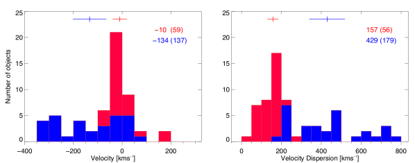
Figure 4: Distribution of velocity (left) and velocity dispersion values (right). In both panels, narrow and second components are indicated in red and blue, respectively. The crosses represent the average values reported on top right, in parenthesis the standard deviation. The horizontal size of the crosses is equal to the standard deviation of the measurements.

4.2 Comparison with previous broad H$\alpha$ detections

In Table LABEL:T_FWHM we summarise the measurement of the FWHM of the broad H$\alpha$ components obtained in the present work (hereafter C18) for ground- and space-based data and previous works. The comparison between our measurements of the FWHM of the broad H$\alpha$ component and those from previous works is discussed in what follows for both space (Sect. 4.2.1) and ground- and space-based data (Sect. 4.2.2). The possible factors generating agreement or discrepancy are discussed in Sect. 5.1.

4.2.1 Space-based HST/STIS measurements

The broad component is required to model the H$\alpha$ line profile for all the 11 LINERs observed with HST/STIS spectroscopy (Sect.4).
In Fig. 6, our measurements of the FWHM of the H$\alpha$ in space-based data are compared to those listed in previous works by BC14 and Constantin et al. (2015) (hereafter C15). The former comparison is particularly instructive as the results are obtained with different analysis of the same data set (Sect. 2.1). The effects of the procedure for line modelling will be discussed in detail in Sect. 5.1.1.
Of the 11 HST/STIS spectra analysed in the present work, only in two cases (NGC 3398 and NGC 4450) the BLR-component was confirmed by BC14. For NGC 4450, the agreement of the FWHM measurements is rather good (within $\pm$ 200 km s^-1). For NGC 3998 our measurement is 15 $\%$ smaller ($\sim$ 800 km s^-1, Table LABEL:T_FWHM). However, this is a particular case: despite the modelling reproduce well the line profiles (Table LABEL:T_rms), the [O I]$\lambda$6300 line is strong but partially truncated (Fig. 23). This compromises the detection of any putative second component in [O I], and hence in H$\alpha$ (Sect. 3.2 ).
In the remaining nine sources, BC14 did not find convincing evidence of a broad component. Specifically, although a broad component must generally be included to achieve a good fit, rather different FWHM values are inferred adopting either [O I] or [S II] lines as reference.
The HST/STIS spectra of nine LINERs of the present sample were also analysed by C15. These authors presented the same dataset as that analysed in this paper but with a different treatment of data in terms of data reduction, stellar subtraction (Sec. 3.1) and line modelling. In particular, C15 used only the [S II] profiles as a template for H$\alpha$-[N II]. However, they allowed multiple components when modelling [S II] to take into account any possible asymmetries of the line profiles and broad wings. In their work, they confirmed the broad H$\alpha$ detection (previously reported by Ho, Filippenko & Sargent 1997a) for all the nine LINERs in common with our sample (Table LABEL:T_FWHM). Of these, NGC 4636 has not been analysed in the present work (Tables LABEL:T_kin and LABEL:T_FWHM) as the data quality is insufficient to proceed to any reliable analysis (see Fig. 7 in BC14).
We found a general agreement (within $\sim$ 400 km s^-1) with the measurements by C15, excluding those cases for which our H$\alpha$-[N II] modelling was less reliable (Table LABEL:T_rms). The match is remarkably good in the cases of NGC 4036 and NGC 5077 (the difference in FWHM is less than 110 km s^-1, Table LABEL:T_FWHM and Fig. LABEL:T_FWHM). A significant discrepancy of about 1900 km s^-1 is found only for NGC 3998.
In this comparison, it has to be noted that the broad component detected by C15 is located at large shift with respect to rest-frame (up to $\sim$ 1200 km s^-1 in the case of NGC 0315) relative to the narrow H$\alpha$. In contrast the shift is generally lower, varying between -300 and 550 km s^-1 (Table LABEL:T_kin), in our measurements (considering both ground- and space-based data).

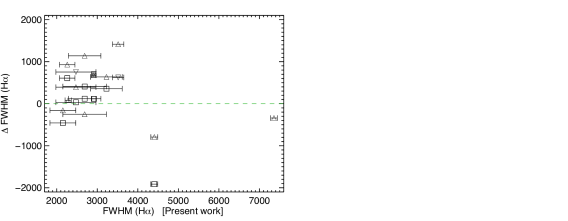
Figure 6: The difference between the FWHM values of the H$\alpha$ broad component measured in space data in the present manuscript and those of previous works, i.e. $\Delta$ FWHM (H$\alpha$), against our measurements (Table LABEL:T_FWHM). Boxes and triangles mark the comparison with the FWHM listed in C15 and BC14. More specifically, upward and downward triangles indicate the FWHM of the broad H$\alpha$ required by the fit using as template for the narrow component the [S II] and [O I] lines, respectively. An additional circle marks those galaxies with a less reliable H$\alpha$ fit (Table LABEL:T_rms). The green dashed line indicates the zero, as reference. Errors in y-axis are not available.

4.2.2 Ground-based measurements

With our CAHA/NOT spectroscopy we confirm the presence of the broad H$\alpha$ component in 7 out of 21 (i.e. 33 $\%$) LINERs-1 of the selected sample, by using mainly S- and M-models and allowing multiple components to reproduce forbidden lines and narrow H$\alpha$ profiles (Sect. 4). Such a low detection rate of the broad H$\alpha$ component disagrees with that from the analysis of spectra from the Palomar Survey (i.e. 100 $\%$, Ho, Filippenko & Sargent 1997a, HFS97 hereafter).
In the common cases of broad-component detection, the measurement of the FWHM for such broad components are somewhat different (Table LABEL:T_FWHM). Specifically, in two cases (namely NGC 2787 and NGC 4636) the FWHM in Palomar observations is larger by a factor of $\sim$ 1.6 and $\sim$ 1.1, respectively (Table LABEL:T_FWHM). In four cases (NGC 0315, NGC 3718, NGC 4750 and NGC 5077) our measurements indicate a larger FWHM of the broad component (by a factor $\sim$ 1.2). In the remaining case (NGC 3642), our FWHM-measurement is larger by a factor $\sim$ 2.5.

Table 7: FWHM of the H$\alpha$ broad component from different works.

ID	Obs.	C18	HFS97	BC14	C15
		km s-1	km s-1	km s-1	km s-1
NGC 0266	CAHA †	-	1350	-	-
NGC 0315	NOT	[2474 $\pm$ 389]	2000	-	-
	HST †	3227 $\pm$ 495	-	2590	2870
NGC 0841	CAHA	-	1350	-	-
NGC 1052	NOT	[-]	1950	-	-
	HST	[2916 $\pm$ 52]	-	2240 (2210)	2800
NGC 2681	CAHA	-	1550	-	-
NGC 2787	CAHA	1277 $\pm$ 195	2050	-	-
	HST ‡	2282 $\pm$ 75	-	2200	-
NGC 3226	CAHA	-	2000	-	-
NGC 3642	CAHA	[3158 $\pm$ 565]	1250	-	-
	HST †	[2259 $\pm$ 191]	-	1330	1650
NGC 3718	CAHA	2582 $\pm$ 518	2350	-	-
NGC 3884	CAHA †	-	2100	-	-
NGC 3998	CAHA	[-]	2150	-	-
	HST ‡	4407 $\pm$ 85	-	5200	6320
NGC 4036	CAHA	-	1850	-	-
	HST	2474 $\pm$ 595	-	2080 (1720)	2440
NGC 4143	CAHA ‡	-	2100	-	-
	HST	3515 $\pm$ 139	-	2100 (2890)	-
NGC 4278	CAHA	-	1950	-	-
	HST ‡	2689 $\pm$ 537	-	2940	2280
NGC 4438	CAHA	[-]	2050	-	-
NGC 4450	CAHA	-	2300	-	-
	HST	7359 $\pm$ 80	-	7700	-
NGC 4636	CAHA	2152 $\pm$ 429	2450	-	-
NGC 4750	CAHA	2367 $\pm$ 106	2200	-	-
NGC 4772	CAHA	-	2400	-	-
NGC 5005	CAHA	[-]	1650	-	-
	HST †	2152 $\pm$ 318	-	2310	2610
NGC 5077	CAHA	2797 $\pm$ 560	2300	-	-
	HST †	2689 $\pm$ 400	-	1550	2570

Notes. Measurements of the FWHM of the broad H$\alpha$ component. These are from: C18 (present work, see also Table LABEL:T_kin), HFS97 (ground Palomar data), BC14 and C15 (both from space HST/STIS observations). For the measurements by BC14, in parenthesis we indicate the FWHM of the broad H$\alpha$ required by a fit obtained using [O I] as template for narrow lines. The other measurements were done using [S II] lines as reference. ‘ID’: object designation as in Table 1. ‘Obs’ stands for the origin of the optical data. ^† and ^‡ symbols and square brackets are as in Table LABEL:T_kin.

5 Discussion

5.1 Probing the BLR in type-1 LINERs

The analysis of Palomar spectra by Ho, Filippenko & Sargent (1997a) indicated that all the LINERs in our selected sample show a broad H$\alpha$ component resulting in their classification as LINER-1 nuclei. Nevertheless, with our analysis of ground- and space-based data sets, we found discrepant results. On the one hand, with the analysis of ground-based observations, we found the detection rate for the broad H$\alpha$ component to be only 33 $\%$ (Sect. 4). This result questions their previous classification of type-1 LINERs. On the other hand, for all the LINERs with HST/STIS spectra and in common with BC14, the observed line profiles require the broad H$\alpha$ component for a satisfactory modelling.
The lack of detection of the broad H$\alpha$ component in LINERs could be due to the absence of the BLR or its undetectability (e.g. the broad emission is too weak and/or highly contaminated by the starlight). If the BLR is present in LINERs, as it was supposed to be in our sample, its detectability (via the broad H$\alpha$ component) is sensitive to two main factors: modelling and observational effects.

5.1.1 Effect of different modellings

The two main factors related to modelling that might affect the detectability of the BLR component are: the stellar subtraction and the strategy adopted for the line modelling. The former determines the accuracy of achievement of a pure ISM spectra, which is particularly relevant for a proper kinematic decomposition. This effect is expected to be rather more relevant as the slit width increases (thus for our ground-based data). On the other hand, the strategy adopted for the emission line fitting is closely related to both the identification of the model that best fits the emission lines (i.e. in terms of number of Gaussians) and the underlying physics of the assumed models (i.e. the choice to use [S II] or [O I] or both as template for H$\alpha$-[NII]).

The comparison between our measurements and those by BC14 provides the optimal framework to test our line fitting procedure (Sect. 3.2). Specifically, this comparison is not biased by any issue about the starlight subtraction or observational effects (e.g. possible AGN variability, see also Sect. 5.1.2) as we stress that the results are obtained with two different analyses of the same data set. Hence, we checked if our procedure for the line modelling is able to reproduce the fluxes listed in BC14 and Balmaverde et al. (2016) for H$\alpha$ and forbidden lines, respectively. Fig. 7 presents the results of this test.
The comparison is rather positive as our measurements match those of Balmaverde et al. (2016) within 20 $\%$ considering [S II] lines (crosses in Fig. 7). Slightly less agreement ($\sim$ 30 $\%$) is found for [O I] and [N II] and the largest scatter is seen for H$\alpha$ (Fig. 7, bottom panels). Overall, the more evident exception is NGC 3998 whose line modelling is somewhat complicated (Fig. 23).
We found a rather good agreement (within 30 $\%$) also when comparing the different contribution of the broad component of H$\alpha$ to the H$\alpha$-[N II] blend and to the total H$\alpha$ emission i.e. f_blend and f_Hα, respectively (Fig. 7, top panels). These contributions are defined as: f_Hα =  F(H$\alpha$_B)/F(H$\alpha$_N(+S)) and f_blend =  F(H$\alpha$_B)/F(H$\alpha$_N+B(+S)+F([N II]_N(+S)), where F is the line flux and ‘B’, ‘N’ and ‘S’ stand for broad, narrow and second (if present) components. The discrepancy is large ($\sim$ 40-50 $\%$) for NGC 3642 (due to an uncertain modelling, Fig. 20) and NGC 5077 (Fig. 34).
Although, in the analysis by BC14 they tested both the S- and O-models (Sect. 3.2) not finding a convincing piece of evidence supporting the presence of the BLR (Sect. 4.2.1). However, it is important to note that they did not consider multiple Gaussians when fitting the forbidden lines used as template. In the case of a broad and asymmetric profile of the selected template ([S II] and [O I]), one Gaussian is certainly an oversimplification. Therefore, the width of each single narrow Gaussian component used for the selected template tend to be overestimated hampering the modelling of H$\alpha$ components (e.g. resulting in a spurious detection of the broad component). This might be partially at the origin of the mismatch seen in few cases (e.g. NGC5077) in Fig. 7.
As mentioned above, the effects of the stellar subtraction are absent when comparing our results with those by BC14. However, these effects (along with other factors Sect. 4.2) could still play a role in the comparison with the work by C15, who removed the stellar continuum from HST/STIS spectra. Despite this, the nice agreement of the FWHM of the H$\alpha$ broad component (Fig. 6 and Table LABEL:T_FWHM) seems to indicate that the starlight subtraction only moderately affects the measurements in HST/STIS spectroscopic data.

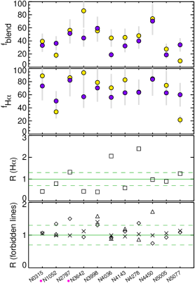
Figure 7: Comparison between the results obtained from the proposed line fitting procedure applied to space-based data with the measurements from BC14 and Balmaverde et al. (2016). From bottom to top: the ratio (R) of the flux of the narrow component (plus the second component, if present) used to model forbidden lines and narrow H$\alpha$ in the present manuscript and the above mentioned previous works, f_Hα and f_blend (see text). These latter are expressed in terms of a percentage. In the two bottom panels, the different species: [O I], [N II], [S II] and H$\alpha$ are marked with triangles, diamonds, crosses and boxes, respectively. Green continuos and dotted lines indicate unity and $\pm$ 30 $\%$. In the top panels, purple and yellow mark the values of f_Hα and f_blend in the present work and those in the reference works, respectively. Grey bars indicate 30 $\%$ uncertainty. Pink circles (near IDs on the x-axis) mark those cases with less reliable line-modelling (Table LABEL:T_rms).

We performed the same kind of comparison for our ground-based data considering the results from HFS97. We mitigate possible slit-aperture effects by considering aperture-corrected fluxes (i.e. normalized to a 1″.0 $\times$ 1″.0 aperture). Nevertheless, we found a discrepancy (of about 40-50 $\%$, typically) between the measurements of forbidden lines and narrow H$\alpha$ in different ground-based observations. The different detection rate of the broad H$\alpha$ component between the present work and that by HFS97 (i.e. 33 $\%$ vs. 100 $\%$, respectively, Sect.4) prevents the one-to-one comparison of the measurement of f_Hα and f_blend.
Moreover, the interpretation of such a comparison is not as straightforward as for space-based data, since besides the strategy adopted for the line modelling, a number of factors may contribute to the possible discrepancies including: starlight subtraction, the difference in the slit-PAs and possible AGN variability. We already discussed the possible biases introduced with the modeling of the stellar continuum (Sect. 3.1). Effects related to the differences in the slit-PAs and the possible AGN variability will be discussed in a dedicated section (Sect. 5.1.2).

Thus, our procedure for the line modelling is able to produce overall flux measurements the BLR component consistent with previous works (e.g. no over/under-fitting). Nevertheless, the results obtained in the present comparison and those presented in Sect. 4.2 indicate a significant impact of the line modelling on the detection and properties of the BLR component.

5.1.2 Observational effects

The broad H$\alpha$ component is expected to be relatively more dominant as the slit width decreases since for narrower slit observations the contamination of starlight and of narrow lines is reduced, favoring the detection of the BLR-component. On the one hand, the BLR could be present but visible only at HST/STIS scales, if dilution effects from the host galaxy have a dominant role. On the other hand, the BLR could be intrinsically absent. In this case, finding a broad component could be the result of the combined effects of questionable starlight decontamination and of an inappropriate choice of the model for emission lines (Sect. 5.1.1).
For the present work, aperture effects are likely more significant when comparing ground- and space-based data. Indeed, the HST/STIS aperture is significantly smaller ($\leq$0.$\arcsec$2, BC14) than the TWIN/ALFOSC aperture in our data (Table 2). Aperture effects are expected to be smaller when comparing ground-based data sets. Specifically, CAHA/TWIN and NOT/ALFOSC slit apertures are similar but slightly smaller (a factor 2-3 in size, typically, Table 2) than the 2″.0$\times$4″.0 aperture in the Palomar Survey (Filippenko & Sargent, 1985).
In Sect. 4.1, we briefly compare ground- and space-based narrow and broad emission lines measurements finding differences in terms of the assumed model and the number of components (Table LABEL:T_kin). These differences could be due to a sharp variation of velocities toward the SMBH that could be related to the presence of non-rotational motions such as outflows. Indeed, the outer parts and cores of outflows (that are mapped in a different way in different slits) might behave otherwise leading to some velocity and velocity dispersions gradients. An alternative explanation is a complex stratification in density and ionization of the NLR. Observational effects could originate the different detection rate and FWHM measurements of the BLR component in our ground- and space-based data.

Considering the ground-ground comparison, we mitigate aperture effects via flux normalization, as mentioned in Sect. 5.1.1. Despite this, discrepancies remain when comparing narrow and broad lines measurements.
In this comparison, the differences in the slit PA could be also relevant, as weak spectral features could be diluted or contaminated by potential nuclear H II regions. Therefore, we checked if any trend exists between the difference in the slit-PAs and those values of f_Hα and f_blend, finding no correlations. The presence of either strong non-rotational motions or complex phenomena such outflows might also complicate the emission lines fitting especially in case of severe H$\alpha$-[N II] or [S II] blending.

With the present data sets, it is not possible to quantify any effect related to possible AGN-variability which does not occur at similar time-scale in different objects of the same AGN family (e.g. Younes et al. 2011; Hernández-García et al. 2014, 2016).

5.2 Classification of the velocity components

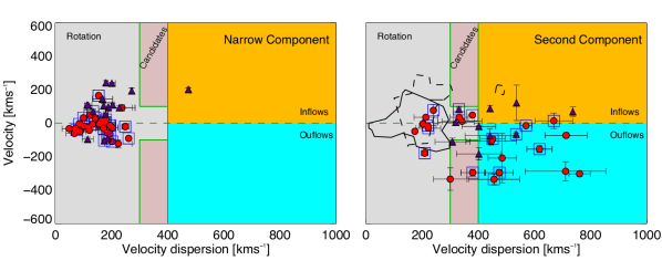
Figure 8: Observed velocity dispersion - velocity ($\sigma$-V plane) plane for narrow (left) and second (right) components. Red circles an purple triangles mark the measurements from ground- and space-based data, respectively. An additional blue box marks those LINERs for which the fitting of the H$\alpha$ profile is less reliable (Table LABEL:T_rms). In the right panel, we report the measurements of the narrow component with contours (continuos and dashed lines are for ground- and space-based data, respectively). The different coloured areas marked with continuous and dashed green lines indicate the location of our measurements that could be explained by rotation (gray), outflows/inflow candidates (pink), outflows and inflows (orange and light blue, respectively). See Sections 5.2 and 5.3 for details. Note that the number of objects with less reliable fit in this figure are different from those in Fig.7, where only HST data are considered. For NGC 1052, 4 points are used to represent the different model components (see Table 3).

To interpret the physics behind the line modelling proposed in Sect. 3.2, we consider the measurements of the kinematics (velocity and velocity dispersion) from the nuclear spectra in both ground- and space-based data sets (Table LABEL:T_kin). In Fig. 8, we present the distribution of the velocity for narrow and second components as a function of their velocity dispersion ($\sigma$-V plane).
We consider the kinematics of the narrow and second components from the lines used as template, i.e. [S II] and [O I] (Table LABEL:T_kin). We recall that for all the models proposed in Sect. 3.2, H$\alpha$ is tied to [O I], thus the components used to fit these emission lines share the same classification. Nevertheless, the classification of the components used to model [N II] lines is not always linked to that of either [S II] and [O I] as M-models encompass two different alternatives for [N II] (Sect.3.2). Therefore, in our classification scheme we therefore neglect the kinematical information inferred from [N II], for simplicity.
For a more accurate analysis, we combine these results with the measurements of velocities from the 2D spectra (before the extraction of the nuclear one, i.e. measuring individual sections). Specifically, we inferred the amplitude of the velocity-field of the ionised gas using the position-velocity diagrams presented in Fig. 35 (Appendix B).
Since the observations were performed without any orientational prescription (Sect. 2), it is possible that the kinematic components associated to the regular rotation might be present in the line of sight. Thus, we estimate the maximum broadening of emission lines due to rotation, as the peak-to-peak amplitude of the ionised-gas velocity rotation curve (Fig. 35), which is generally lower than $\sim$ 400 km s^-1. This is a conservative estimate as, generally, larger values (i.e., amplitudes of $\sim$ 300-400 km s^-1) are observed outside the region used to obtain the nuclear spectra (Table 2 and Fig. 35). Indeed, considering only the individual spectra used to obtain the final (nuclear) one, the velocity amplitude of the ionised gas rotation is generally smaller (up to $\sim$ 300 km s^-1). These estimates are in fair agreement with the spectroscopic measurements of the velocity amplitude of the ionised gas rotation for samples of nearby spirals (GHASP survey, Epinat et al. 2010) and early type galaxies (ATLAS^3D, Ganda et al. 2006; Cappellari et al. 2007).
The typical values of velocity dispersion for the narrow components are well below the two limits, 300 and 400 km s^-1, estimated in the case of line-broadening due to rotation (Fig. 8 right); velocities are typically rest-frame (i.e. 0 $\pm$ 50 km s^-1) except for a few cases (see Table LABEL:T_kin). Therefore, a simple interpretation is that the line widths of the narrow component can be explained by rotation.
The distribution of the kinematic measurements for the second component is more spread in the $\sigma$-V plane than that for the narrow component (Fig. 8 left). This behaviour is also evident in Fig. 4. Those kinematic components with $\sigma$ $\sim$ 400-800  km s^-1 (that cannot be produced by rotation) are likely associated to turbulent non-rotational motions. Similarly, those components with 300 $<$ $\sigma$ $<$ 400 km s^-1, with velocities larger than $\pm$ 100 km s^-1 are difficult to interpret as due to rotation. Therefore, these components are considered as candidates for non-rotational motions. All the emission line components associated to non-rotational motions (and candidates) will be discussed in Sect.5.3.
Finally, the broad H$\alpha$ component is interpreted as a signature of the presence of the BLR (as mentioned already in Sect. 3.2).

For the sake of homogeneity, we adopted the same criterion to classify the velocity components for both ionised and neutral gas phases. The motivations are twofold. First, the NaD detection is robust only in a minor fraction of our LINERs (i.e. 8/21, 38 $\%$, Sect. 3.3). Second, the individual spectra in the region used to extract the nuclear one lack the required S/N for stellar modelling and line fitting. Hence, with the present data set it is impossible to determine the neutral gas rotation curves, as done for emission lines (Fig. 35). Therefore, according to the classification scheme for the velocity components in emission lines, all the neutral gas kinematics can be interpreted as due to rotation, except for the case of NGC 0315 (candidate for non-rotational motion).
The neutral gas velocity dispersion is typically larger than that of the ionised-gas (narrow component). This might indicate the presence of either mild non-rotational motions of the neutral gas in these LINER-nuclei (as discussed in Sect. 5.5) or two different rotating discs (ionised and neutral). Specifically, the neutral gas disc rotation does not necessarily follow that of the ionised disc; with the former possibly either lagging or being dynamically hotter and thicker compared to the latter (as seen in nearby U/LIRGs, Cazzoli et al. 2014, 2016).
We discuss individual cases in Appendix  B, taking into account the possible differences and analogies of ionised and neutral gas kinematics.

5.3 Non-rotational motions

We identify four areas in the $\sigma$-V plane (Fig. 8) occupied by the kinematic measurements for the ionised gas that we associate with:

• rotation: in the region limited by $\sigma$ $<$ 300 km s^-1, and by 300 $<$ $\sigma$ $<$ 400 km s^-1 and 100 $<$ $\mid$ V $\mid$ km s^-1 (grey);

• candidates for non-rotational motions: in the regions limited by 300 $<$ $\sigma$ $<$ 400 km s^-1 and $\mid$ V $\mid$ $<$ 100 km s^-1 (pink);

• non-rotational motions within the region limited by $\sigma$ $>$ 400 km s^-1, at both negative (blue) and positive velocities (yellow).

These are conservative criteria considering both the 2D rotation curves (Fig. 35) and the kinematics of all the components in our nuclear spectroscopy (see Sect. 5.2 for details).
In Table LABEL:class_sum, we summarise the present classification. In the following, we explore the possibility of rotation (R), candidates for non-rotational motions (C) and of those non-rotational motions being produced by outflows (O) or inflows (I) having negative and positive velocities, respectively. It is worth to note that Monte Carlo simulations based on the 3D outflow models by Bae & Woo (2016) indicate that intermediate-width lines with positive velocities can also be interpreted as outflow (hence not inflow). This is a consequence of dust obscuration and special prescriptions of the outflow geometry (e.g. biconical outflows). In this paper we assume the outflow/inflow interpretation and classified the line-components accordingly. However, with the present data set it is not possible to infer outflow opening angles and geometries and hence producing a detailed model for the outflows is beyond the aim of this work.

The kinematics of the narrow component can be interpreted as rotation in all cases (Fig. 8 left). Although, the data points for the second component can be found in all the four areas (Fig. 8 right) encompassing all the proposed possibilities with [O I] and [S II] classifications being different in 5 cases (NGC 1052, NGC 3642, NGC 4143, NGC 4278 and NGC 4450; Table LABEL:class_sum). Taking into account the various possibilities for second components, the final adopted criterion for claiming a possible interpretation as outflow/inflow (rotation) is that both [S II] and [O I] second component are classified as outflow/inflow (rotation) in Fig. 8 (see also Table LABEL:class_sum). In those 5 cases (Table LABEL:class_sum) where the wavelength coverage of our data does not allow to probe either [S II] or [O I], the final classification is set equal to that of the only second component of the forbidden line adopted for the line fitting. If non-rotational motions (either outflow or inflow) or a candidate are seen in only one component we consider these putative interpretation as less reliable. The final classification is listed in column 5 of Table LABEL:class_sum.

For ground-based data, this criterion clearly identifies 6 and 3 cases out of 15 with outflows (40 $\%$) and rotation (20 $\%$), respectively (Table LABEL:class_sum). Only one robust case (NGC 4750, Table LABEL:class_sum) of candidate for non-rotational motions has been found. In the remaining five cases (33 $\%$, Table LABEL:class_sum), the classification for [O I] and [S II] is different. Specifically, in all of these five cases, the classification as non-rotational motions (outflows) or candidate held only for [O I] with [S II] being classified as rotation. Conversely, the alternative for which [S II] is classified as non-rotational motions and [O I] rotation never occurs. Such a large prevalence of non-rotational motions or candidate found in [O I] with respect to [S II] (i.e. 10 vs. 5 cases, considering only those cases for which both forbidden lines are present) might indicate that LINERs are only able to power low-ionisation emission-line outflows. A detailed and possibly 2D study with IFS data is needed to investigate further this issue.
There are not systematic studies of outflows in type-1 LINERs via ground-based spectroscopy, but only works of individual cases (e.g. Dopita et al. 2015; Brum et al. 2017). The detection rate of outflows in ground-based data is lower than what found in studies of sample of nearby (z $<$ 0.2) type-2 luminous AGNs and quasars (e.g. Harrison et al. 2014 and Villar Martín et al. 2014) and local (z $<$ 0.1) U/LIRGs (e.g. Arribas et al. 2014) which is typically larger than 70 $\%$.
We found that, generally, the outflow-components have velocities varying from -15 km s^-1 to -340 km s^-1, and velocity dispersions in the range of 450-770 km s^-1 (on average, 575 km s^-1).
In our data set, the components interpreted as outflow have intermediate kinematic properties between outflows observed in AGNs and U/LIRGs. More specifically, the range of velocity is typically smaller than what found in outflows in AGNs but the velocity dispersion values are consistent with e.g. those of turbulent outflowing ionised gas in type-2 AGNs found by Harrison et al. (2012) using IFS observations of [O III]. The kinematics of these outflowing components is more extreme than that of outflows observed in U/LIRGs (e.g. Rupke, Veilleux & Sanders 2005c; Arribas et al. 2014) being the velocities more negative and velocities dispersion much larger.

The same classification criterion applied to the results from space-based data implies a null detection rate for outflows, whereas we found 2 cases out of 7 of rotation and 2 cases of candidates for non-rotational motions (Table LABEL:class_sum). The outflow interpretation is less reliable for NGC 1052 (Fig. 16) while NGC 4450 (Fig. 29) is the only LINER for which the components are classified as outflow ([S II]) and inflow ([O I]). However, in this case the outflow classification is less reliable as the H$\alpha$ broad component contaminates the [S II]$\lambda$6716 line. Data at higher spectral resolution are needed to confirm such intriguing outflow-inflow scenario. We found only one case (NGC 4278, Fig. 27) of inflow (Table LABEL:class_sum).

Excluding the particular case of NGC 4450, the number of detections of non-rotational motions ($\sim$ 30$\%$) is lower than what found for the second components in ground-based data analysis. This is in partial agreement with the study of the H$\alpha$ morphology at HST scales in LINERs by Masegosa et al. (2011) which indicates that outflows are frequent (but not ubiquitous) in LINERs. For the present sample of LINERs, the direct comparison between our results and the H$\alpha$ morphology studied in Masegosa et al. (2011) can be done only in four cases (NGC 0315, NGC 1052, NGC 4278 and NGC 5005). In two cases (NGC 1052 and NGC 5005) the H$\alpha$ emission shows morphological evidence of nuclear outflows (see also Pogge et al. 2000). Strong outflows are also seen in the HST/STIS data via multiple velocity components as reported by Walsh et al. (2008) (e.g. NGC 1052).
A possible explanation of the low detection rate of outflows is that their extended nature (e.g. a nuclear expanding bubble) is not fully captured by HST/STIS spectroscopy with narrow slit ($\leq$ 0.2^′′). The detection of line asymmetries interpreted as outflows could be relatively more difficult as the slit width decreases. Slit-orientation effects might also play a role. Furthermore, issues associated to the wavelength-coverage (Sect. 3.2.2) may affect the detection of line asymmetries in space-based data, especially if these are more frequent in [O I] rather in [S II] as seen from the results obtained in ground-based data (Table LABEL:class_sum).

Table 8: Summary of the classification for the second component.

ID	Obs.	[S II]	[O I]	Final
NGC 0266	CAHA †	-	O	O
NGC 0315	NOT	O	O	O
	HST †	R	-	R
NGC 1052	NOT	R	O	[O]
	HST	R	O	[O]
NGC 2681	CAHA	R	R	R
NGC 3226	CAHA	O	O	O
NGC 3642	CAHA	R	C	[C]
	HST †	-	-	-
NGC 3884	CAHA †	-	O	O
NGC 3998	CAHA	O	O	O
	HST ‡	-	-	-
NGC 4036	CAHA	R	R	R
	HST	-	-	-
NGC 4143	CAHA ‡	R	O	[O]
	HST	R	R	R
NGC 4278	CAHA	R	I	[I]
	HST ‡	I	I	I
NGC 4438	CAHA	R	R	R
NGC 4450	CAHA	R	O	[O]
	HST	O	I	[O]
NGC 4750	CAHA	C	C	C
NGC 5005	CAHA	O	O	O
	HST †	C	-	C
NGC 5077	CAHA	-	-	-
	HST †	C	-	C

Notes. ‘ID’: object designation as in Table 1. We list only those LINERs for which a second component is needed to model the observed line profiles either in ground- and/or space-based spectroscopy. ‘Obs’ stands for the origin of the optical data. ^† and ^‡ symbols are as in Table LABEL:T_kin. ‘R’, ‘O’, ‘I’ and ‘C’ indicate: rotation, outflow, inflow and candidate for non-rotational motions, respectively (see text). The last column report the final classification, where square-brackets indicate a less reliable outflow, inflow or candidate for non-rotational classification.

There are two cases (NGC 1052 and NGC 4278) in which the same classification holds for both the ground- and space-based data. Both second components required to model NGC 1052 share the same classification in the two data sets. The second component in [O I] is classified as outflow, in agreement with the outflow interpretation by Walsh et al. (2008) (with HST/STIS data) and by Dopita et al. (2015) (ground-based IFS data). For NGC 4278 (Fig. 27) the inflow classification holds for all the emission lines in both ground- and space-based data sets (except [S II] in ground-based data, Table LABEL:class_sum). This is particularly interesting as the signature of inflows as a second intermediate component at positive (redshifted) velocities are elusive (e.g. Coil et al. 2011; Rubin et al. 2012) whereas outflows have been observed in a variety of galaxies and at any redshift (Veilleux, Cecil & Bland-Hawthorn 2005 and King & Pounds 2015 for reviews).
We refer to Appendix B for detailed comments on individual cases.

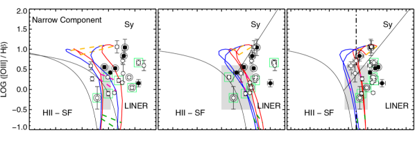
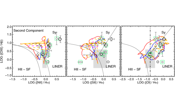
Figure 9: Optical standard BPT diagrams for both narrow and second components (top and bottom panels, respectively) obtained for our ground-based spectroscopy. Circles mark the data points presented in this paper. In the top panels, filled symbols mark those LINERs for which forbidden lines are modelled well with only one Gaussian (i.e. the second component is absent, see Table LABEL:T_kin). In all the panels an additional circle marks those LINERs for which a broad component is required to optimally reproduce the H$\alpha$ line profile (see Table LABEL:T_kin). An additional light-green square marks those galaxies with less reliable fit of H$\alpha$ (Table LABEL:T_rms). Black lines in all diagrams represent the dividing curves between H II star-forming regions, Seyferts, and LINERs from Kewley et al. (2006) and Kauffmann et al. (2003). Gray boxes show the predictions of photoionization models by pAGB stars for Z = Z_☉, a burst age of 13 Gyr (Binette et al., 1994) and ionization parameter values (log U) between -3 and -4. Log U is typically -3.5 in LINERs (Netzer, 2015). The predictions of AGN and shock -ionization models are overlaid in each diagram. Top: Dusty AGN photoionization grid from Allen et al. (2008) with n_el = 100 cm^-3 (Sect. 5.4), for Z_⊙ and 2 Z_⊙, for different power-law spectral indices ($\alpha$ = -1.7, -1.4, blue and red lines) and ionization parameter values (log U = -3.6, -3.0, 0.0, green, pink and yellow dashed-lines). Bottom: Shock+precursor grids from Groves, Dopita & Sutherland (2004) with Z = Z_⊙ and for different n_el. Blue and red curves correspond to models with n_el = 100 cm^-3 and n_el = 1000 cm^-3, respectively (Sect. 5.4). We marked the values corresponding to the minimum and maximum preshock magnetic field allowed in each model. Shock-velocities are from 100 to 800 km s^-1 (yellow dashed lines, Sect. 5.4). In pink is indicated the average shock-velocity for the second component (i.e. $\sim$ 450 km s^-1, Table LABEL:T_sum_kin). The dividing line between weak-[O I] and strong-[O I] LINERs (Filippenko & Terlevich, 1992) is marked in black with a dot-dashed line.

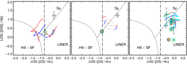
Figure 10: Optical standard BPT diagrams. Coloured circles mark the data point for the second component presented in this paper (as in Fig. 9, bottom-right). Additional symbols as light-green square and black lines are as in Fig.9. We consider predictions of shock-ionization models with Z = Z_⊙ and for different n_el: (100 cm^-3 and 1000 cm^-3) as in Fig.9. The shock+precursor grids are overlaid in each diagrams considering different shock-velocities. Specifically, from left to the right, we consider only shock-velocities relative to the rotation, candidate for non-rotational motions and non-rotational motions, respectively (Fig. 8). Iso-velocities are marked with dashed-lines and colour coded according to the four areas in Fig. 8 (see also Sect.5.3). Similarly, for the colour coding for the observed line ratios (being outflows and inflows marked in light blue and orange, respectively). An additional circle marks those cases for which the final classification is less reliable (Table LABEL:class_sum).

5.4 The underlying physics of the different components

The ionizing mechanism of optical emission lines in LINERs is widely debated and three alternative scenario have been proposed: AGN, pAGB stars and shocks (see Ho 2008 and Netzer 2015 for reviews).
Our data set allows us to classify narrow and second components used to model emission lines combining line-fluxes and kinematics. In Fig. 9, we investigate the location of the line ratios for the narrow and second emission line components onto standard ‘BPT-diagrams’ (Baldwin, Phillips & Terlevich, 1981). These are empirically-derived diagrams based on optical emission line ratios (selected to be essentially unaffected by reddening) that allow to discriminate different ionizing mechanisms. We consider the Kewley et al. (2006) and Kauffmann et al. (2003) curves that allow to distinguish between the locus occupied by star forming systems and AGNs, these separates also the locus between LINERs and and Seyferts. We use the BPT classification to infer the dominant mechanism in LINERs and compare our results with models. Additionally, we consider the criterion for dividing weak-[O I] and strong-[O I] LINERs proposed by Filippenko & Terlevich (1992). In this pioneering work, Filippenko and collaborators separate those two classes of LINERs on the basis of the [O I]/H$\alpha$ ratio which is smaller (larger) than 0.16 for weak-[O I] (strong-[O I], genuine AGN) LINERs. This criterion is particularly helpful as the emission-line spectrum of gas photoionised by the stellar continuum of O-stars can mimic that of LINERs only in the weak-[O I] case. Then, we take into account the kinematical information for each component used to model emission lines and its kinematical classification (Table LABEL:class_sum).
We inferred the electron density (n_el) from the relative flux of the [S II] doublet i.e. by interpolating the curve in Fig. 5.3 of Osterbrock 1989 for T = 10⁴ K (see also Draine 2011). We found for the narrow component: n_el $\leq$ 600 cm^-3 (typically $\sim$ 100 cm^-3), and for the second component: 100 $\leq$ n_el $\leq$ 1000 cm^-3. Moreover, we consider shock-velocities from 100 to 800 km s^-1, as larger values of velocity dispersions are not observed in these LINERs (Table LABEL:T_kin, Figures 4 and 8).
The proposed approach is twofold and is particularly helpful as the different models corresponding to the three possible scenarios (AGN, pAGB stars and shocks) might suffer degeneracies when displayed onto BPTs.

For ground-based data, the line ratios for the narrow component are generally consistent with those observed in AGNs (either Seyfert or LINERs) considering the dividing curves proposed by Kewley et al. (2006) and Kauffmann et al. (2003), excluding as dominant ionization mechanism the star-formation. This is particularly evident in the [O I]/H$\alpha$ diagram (Fig. 9 top-right). The only two exceptions are NGG 3642 and NGC 3884; with the additional case of NGC 3998 whose line ratios lie onto the boundaries between AGNs and star-formation. However, these outliers are mainly seen in the [N II]/H$\alpha$ diagram (Fig. 9, top-left) which suffers of potential problems associated with Nitrogen abundances (Pérez-Montero & Contini 2009, Maiolino et al. 2017 and references therein).
We consider the grids of AGN photoionisation models having n_el inferred from the data and adopting a range of metallicities, ionisation parameter and power-law spectral indices, similarly to Kehrig et al. (2012). We found that these models reproduce well the observed line ratios for the narrow component in $\sim$ 10 cases considering all the diagrams (Fig. 9, top panels).
We then explore, the possibility of (dominant) ionisation by pAGB stars by comparing the observed data points with the models proposed by Binette et al. (1994). We note that these models cannot reproduce the large [O III]/H$\beta$ ratios (e.g. between 0.6-1.2, in log units) for the narrow component in six cases; and that a large overlap between pAGBs-stars and AGN models exists. This overlapping might result in an ambiguous classification in at least six cases (Fig. 9, top panels). Hence, we attempt to break such as degeneracy introducing the additional criterion for weak-[O I] and strong-[O I] LINERs proposed by Filippenko & Terlevich (1992). By combining the selected pAGBs-models and the [O I]/H$\alpha$-criterion, the area corresponding to the stars as genuine dominant mechanism of ionisation is thus reduced. The observed line ratios of the narrow component are generally above the 0.16 threshold (-0.8 in log units) for identifying strong-[O I] LINERs. The only exception is NGC 0266; with two additional cases (NGC 2681 and NGC 4143) whose [O I]/H$\alpha$ ratios are $\sim$ 0.16 (lying onto strong/weak -[O I] dividing line, Fig. 9 top-right).
As a further test, we also checked the possibility of the shock-ionization as the dominant mechanism for producing optical lines in LINERs using the shock+precursor models by Groves, Dopita & Sutherland (2004) with n_el = 1 cm^-3 and n_el = 100 cm^-3. However, these shock-models are able to reproduce the observed line ratios only in a smaller number of cases (typically less than five). This indicates that shocks are not the dominant mechanism but they could be however important in LINERs.
The kinematics of the narrow component can be explained by rotation in all cases (Sect.5.3).
All together these results strongly exclude the pAGBs stars scenario in favor of the AGN-ionisation as dominant mechanism of ionisation for the narrow component in these LINERs with shocks being however relevant.

The location onto BPTs of the line ratios for the second component excludes the star-formation as the dominant mechanism of ionisation (Fig. 9 bottom). This is especially evident in the [O I]/H$\alpha$ diagram (as for the narrow component) with the majority of the data points lying in the LINER-area (Fig. 9, bottom-right). The only exceptions are NGGC 4036 in both [N II]/H$\alpha$ and [S II]/H$\alpha$, and NGC 3998 only in the [N II]/H$\alpha$ one (Fig. 9, bottom panels).
The [O III]/H$\beta$ line ratios for the second component are larger with respect to those of the narrow component being generally above 0.6 (in log units) disfavoring the pAGB scenario. In addition, the [O I]/H$\alpha$ ratios of the second component are well above the 0.16-threshold supporting the strong-[O I] nature of these LINERs.
We attempted to reproduce the observed line ratios for the second component with the shock-models by Groves, Dopita & Sutherland (2004) with n_el = 100 cm^-3 and n_el = 1000 cm^-3 (Fig. 9, bottom) as tested for the narrow component. The match between the shock models and data points occurs differently for low and high ionization lines (e.g. Chisholm et al. 2016). Therefore, we mainly focus in the [O I]/H$\alpha$ diagram as it is the most reliable among standard optical BPTs for studying shocks (Allen et al., 2008). We found that generally the selected models are able to reproduce the observed data points (except two cases, Fig. 9, bottom-right).
The kinematic classification of the second component shows different possibilities from rotation to strong non-rotational motions, with the latter being the most frequent (Fig. 5.2, Sect.5.3 and Table LABEL:class_sum). In the following, we explore the connection between the kinematics of the second component and its dominant ionization mechanism by plotting colour-coded BPT-diagrams. Specifically in Fig. 10, we combine the data points and models for the [O I]/H$\alpha$ diagram with the kinematical classification shown in Fig. 8 (as colour coding) and summarised in Table LABEL:class_sum.
Shocks models (grid at low velocities, Fig. 10 left) are able to reproduce the observed line ratios in two (NGC 4036 and NGC 4438) out of three cases for which the component is classified as rotation. This possibly indicates the presence of mild-shocks associated to the ionised gas rotation (which could be somewhat perturbed). In the case of NGC 2681, the grid of shock models could still reproduce the observed line ratios (Fig.9, bottom-right) but at velocities of $\sim$ 600-700 km s^-1 hence much larger than observed (Table LABEL:T_kin, Fig. 10 left).
Similarly to the case of NGC 2681, shocks models (Fig.9 bottom-right) are able to reproduce the observed line ratios for those two cases classified as candidate for non-rotational motions (NGC 3642 and NGC 4750). However, their line ratios are found at either lower or larger velocities than observed (Fig. 10 middle).
The selected shocks models are generally able to reproduce the observed line ratios within errors of the second component with the only exception of NGC 3998 (Fig. 10, right).
These results are in agreement with studies based on IFS observations of nearby LINERs (e.g. NGC 1052, Dopita et al. 2015) and local U/LIRGs (e.g. Ho et al. 2014) showing that outflows are usually associated with shocks that excite optical emission lines with enhanced line ratios.
For the unique case of inflow (NGC 4278, Table LABEL:class_sum), the selected models cannot reproduce the observed line ratios (Fig. 10, right). However, the corresponding data points, at low [O III]/H$\beta$ and large [O I]/H$\alpha$ ratios, are well reproduced by shock-models with the same parameters as those considered in this analysis but without precursor. These shock-models are not shown in Fig.10 for clarity, therefore we refer to Groves, Dopita & Sutherland (2004).

Unfortunately, we cannot use the BPT diagrams to study the possible ionization mechanism of the component found in the analysis of HST/STIS data, as only the red bandpass is available to us. Despite this, the [N II]/H$\alpha$, [S II]/H$\alpha$ and [O I]/H$\alpha$ ratios give helpful limits to constraint the dominant mechanism of ionization considering the dividing lines between ionization from AGN and star formation.
On the one hand, the ranges of values for the [N II]/H$\alpha$ and [S II]/H$\alpha$ ratios are particularly large for attempting to constraint the dominant ionisation mechanism. Specifically, these ranges are: -0.4 - 0.8 and -0.6 - 0.1 for [N II]/H$\alpha$ and [S II]/H$\alpha$ ratios, respectively, for the narrow component; and -0.5 - 0.6 for the second one for both ratios. On the other hand, the ranges for the [O I]/H$\alpha$ ratio are -0.7 - 0.1 and -0.4 - 0.1, for the narrow and second component, respectively. Thus, these [O I]/H$\alpha$ ratios derived from the analysis of HST/STIS data are outside the region which identifies star formation as the dominant ionization mechanism (favoring the AGN scenario). Moreover, they also indicate that those nuclei are already strong-[O I] LINERs (according to the criterion proposed by Filippenko & Terlevich 1992) at HST/STIS scales.

5.5 A lack of neutral gas outflows in type-1 LINERs?

In Sect. 3.3 we described for the first time the detection of the neutral gas in the nuclear region of the selected type-1 LINERs via the modelling and the analysis of the NaD absorption. This is novel as our sample is composed by low-luminosity AGNs not classified neither as starbursts or U/LIRGs, having SFR  $\leq$ 0.5 (calculated from H$\alpha$ luminosity, Table 2 in HFS97) and log(L_IR/L_☉) $\leq$ 8-9 in many cases (e.g. Sturm et al. 2006). The large majority of previous works focused on starbursts (e.g. Heckman et al. 2000) or U/LIRGs (e.g. Rupke, Veilleux & Sanders 2005c; Cazzoli et al. 2016) on the basis of long-slit and IFS observations. The analysis of the neutral gas component of ISM (via NaD) in AGNs has been done only for small samples of U/LIRGs with a Seyfert nucleus or quasars (e.g. Rupke, Veilleux & Sanders 2005b, Krug, Rupke & Veilleux 2010 and Villar Martín et al. 2014).
According to the classification scheme proposed in Sect. 5.2 all the neutral gas kinematic components (except one) could be interpreted as rotation. The neutral gas velocities (Table 5) are roughly consistent with those of neutral gas discs (detected via NaD absorption) in e.g. U/LIRGs (Cazzoli et al., 2016) but with a larger velocity dispersion considering average values (87 vs. 220 km s^-1).
The possible explanation of the lack of neutral gas outflows, or more in general of non-rotational motions, is twofold. First, the neutral component in outflows is possibly less significant in AGNs or quasars than in starbursts galaxies and U/LIRGs, as argued by Villar Martín et al. (2014). Secondly, such null detection rate might be a consequence of the conservative limits we assumed for kinematic components in emission lines (Sect. 3.3). As ionised and neutral gas correspond to different phases of the outflows, these may have a different kinematics (e.g. Cazzoli et al. 2016). Neutral gas kinematical components with large velocity dispersions ($>$ 300-400 km s^-1) are found only in Seyferts or the most luminous ULIRGs (Krug, Rupke & Veilleux 2010; Martin 2005). Furthermore, the velocity thresholds assumed to identify outflows are generally lower (of the order of 50-100 km s^-1). If the adopted limits are relaxed, and we assume those for identifying outflows assumed in Cazzoli et al. (2016), i.e. V $<$ -60 km s^-1 and $\sigma$ $>$ 90 km s^-1, we would have found three cases for possible outflows (NGC 0266, NGC 1052 and NGC 4750). Likewise, NGC 0315 would have been classified as inflow.

6 Summary and conclusions

We analysed a sample composed by the 22 nearby (z $<$ 0.025) type-1 AGN-LINERs from the Palomar Survey, covering the best-defined sample of this kind (HFS97). We studied the properties of the ionised and neutral gas in these LINERs on the basis of CAHA/TWIN, NOT/ALFOSC, and HST/STIS optical long-slit spectroscopy.
First, for each LINER observed via ground-based spectroscopy we modeled and subtracted the stellar continuum to obtain a pure ISM spectrum. Second, we modeled a set of emission lines in both ground- and space-based data testing various models in order to explore the presence of an H$\alpha$ broad component (indicative of an AGN) and to study the kinematics and the ionisation mechanism for the ionised gas. Finally, we modelled the NaD ISM-absorption doublet with Gaussian components to investigate the neutral gas in these LINER nuclei.
We excluded NGC 4203 from the analysis as its very broad and double peaked H$\alpha$ profile requires a more detailed modelling.
The main conclusions can be summarised as follows:

1. The AGN nature of type-1 LINERs. The H$\alpha$ broad component indicative of the presence of the AGN is elusive in our ground-based spectroscopy with a detection of only 7 out of 21 cases (33 $\%$ of detection rate). The measured FWHM of the broad component ranges from 1277 km s^-1 to 3158 km s^-1 (2401 km s^-1, on average). Conversely, the broad component in HST/STIS spectra is ubiquitous, and its FWHM values are between 2152 km s^-1 and 7359 km s^-1 (3270 km s^-1, on average). The broad component is seen in both ground- and space-based data in four cases. The detectability of the BLR-component is sensitive to modelling and observational effects. On the one hand, a broad component could be the result of the combined effects of questionable starlight decontamination and of an inappropriate choice of the template for the H$\alpha$-[N II] blend. Additionally, a single Gaussian fit of template forbidden lines is an oversimplification in many cases. This assumption has a significant impact on the detection and the determination of the properties of the BLR component. However, from our analysis, it seems that aperture and slit-PA differences are not very relevant when comparing ground-based data.
   

2. Multiple component fitting of forbidden lines and stratification of the NLR. For ground-based data, in 15 out of 21 cases the modelling of forbidden lines requires two components. Similarly, for space-based data, we found that two components in forbidden lines are needed to reproduce the observed line profiles in 7 out of 11 cases. However, we do not always find full agreement between the selected models and components used to fit emission lines for the two data sets. When we are able to test all the proposed models, in 9/19 (5/7) cases for ground (space) -based data, we found a prevalence of best fits obtained with the Mixed models (those with different properties for [S II] and [O I], see Sect. 3.2) that take into account differences in critical densities and shock-enhancements. This suggests that the NLR stratification is often present in type-1 LINERs. [O I] lines profiles are typically broader than [S II] (up to a factor of $\sim$ 3, considering second components).
   

3. 2D Ionized gas rotation and rotational broadening. The peak-to-peak velocity amplitude of the ionised gas rotation is generally lower than $\sim$ 300-400 km s^-1 in fair agreement with the spectroscopic measurements of the velocity amplitude of the ionised gas rotation for samples of nearby spirals and early type galaxies. The broadening due to the possible superposition of several rotation components is (conservatively) estimated to be up to 400 km s^-1.
   

4. Kinematics of narrow and second components of emission lines. For the narrow component, velocities are typically rest-frame (i.e. 0 $\pm$ 50 km s^-1, except a few cases) and velocity dispersion values are smaller than 300 km s^-1. For the second components the velocity range is large (from -350 km s^-1 to 100 km s^-1). The velocity dispersions vary between 150 and 800 km s^-1 (429 km s^-1, on average) being generally broader than narrow components. Generally, for space HST/STIS data, except for a few cases, narrow components have velocities between -100 and 200 km s^-1, being the average velocity dispersion 176 km s^-1. The velocity of the second component ranges from -200 to 150 km s^-1 with velocity dispersion values between 300 and 750 km s^-1 (433 km s^-1, on average).
   

5. Kinematical classification of the emission line components. Four areas in the $\sigma$-V plane are defined for different kinematical interpretations with the following limits (expressed in km s^-1): a) rotation: either $\sigma$ = [0, 300] or $\sigma$ = [300, 400] and V = [-100, 100], b) candidate for non-rotational motions: $\sigma$ = [300, 400] and $\mid$ V $\mid$ $>$ 100 and c) non-rotational-motions (as outflows or inflows): $\sigma$ $>$ 400. We adopt the interpretation that blue/redshifted lines might be produced by inflows/outflows. However integral field spectroscopy would be required to confirm/discard such a scenario. For both ground- and space-based data, the kinematics of the narrow component can be explained with rotation in all cases whereas that of the second components encompass all possibilities. Furthermore, the classification might be different for [S II] and [O I], being non-rotational motions more frequently traced by [O I]. Taking these results into account, the final adopted criterion for claiming the possible interpretation as an outflow/inflow (rotation) is that both [S II] and [O I] second component are classified as outflow/inflow (rotation).
   

6. Non-rotational motions. From our ground-based data, we identified 6 out of 15 (40 $\%$) cases that may be interpreted as reliable outflows. Outflow-components have velocities varying from -15 km s^-1 to -340 km s^-1, and velocity dispersions in the range of 450-770 km s^-1 (on average, 575 km s^-1). These values are intermediate between those for outflows observed in AGNs and starbursts (as U/LIRGs). We did not interpreted as outflows any case in HST/STIS data. These results partially disagree with studies of the H$\alpha$ morphology in LINERs which indicate that outflows are frequent in LINERs. The possible explanation is twofold. First, the extended nature of outflows is not fully captured by the HST/STIS spectra. Second, if outflows are more frequent in [O I] than [S II] (as seen for ground-based data), the absence or truncation of [O I] in 8 of the space-based spectra hinders the interpretation. We found one case (NGC 4450) for which the inflow interpretation held for all the emission lines (except [S II]) in both ground- and space-based data sets.
   

7. Ionization mechanisms. By combining the location of line ratios onto BPTs and the empirical dividing curves between H II star-forming regions, Seyfert and LINERs, theoretical models of AGNs, pAGBs and shocks -ionisation and the weak/strong -[O I] classification, we exclude the pAGB scenario in favor of the AGN as the dominant mechanism of ionisation of the narrow component in these LINERs. The [O I]/H$\alpha$ values for space-based spectra also support this result. Generally, the line ratios for the second component are well reproduced by shock-models. In particular, we combined line ratios with our kinematical classification for the most reliable optical BPT diagram for shocks (i.e. [O I]/H$\alpha$) to confirm the presence of shocks associated to outflows.
   

8. Neutral gas in type-1 LINERs. For the NaD absorption lines, in 7 out of 8 cases, a single kinematic component already gives a good fit, suggesting that if a second component exists in these galaxies, it is weak. The velocities of the narrow components vary between -165 and 165 km s^-1; the velocity dispersions are in the range 104-335 km s^-1 (220 km s^-1, on average). The range of velocities and velocity dispersions of the neutral gas are slightly larger than what we found for narrow components in emission lines in both ground- and space-based spectroscopy, but smaller than those found for second components in both sets of data. The result of our line modelling suggests that the neutral gas is generally optically thick in these objects. Generally, the neutral gas kinematical components could be interpreted as rotation. The neutral gas velocities are roughly consistent with those of neutral gas discs (detected via NaD absorption) in U/LIRGs but with a larger velocity dispersion considering average values. The possible explanation of the lack of neutral gas outflows, or more in general of non-rotational motions, is twofold. First, the neutral component in outflows is possibly less significant in AGNs or quasars than in starbursts galaxies and U/LIRGs. Second, such null detection rate might be a consequence of the conservative limits we assumed for kinematic components in emission lines, as the different phases of outflows might have different kinematics (see Sect. 5.5).
   

Therefore, the kinematics and fluxes that we derive from our spectroscopic data provided valuable insight into our general understanding of LINERs, in terms of AGN-classification, dominant ionisation mechanism, kinematics and the possible presence of multiphase-outflows.

Appendix A Stellar modelling

Table 9 summarises the details of the optical observations for the ten non-active galaxies selected from the work of HFS97 (See Sections 2 and 3.1).
Fig. 11 presents the stellar continuum modelling of the spectra of template galaxies obtained with the pPXF procedure. The spectrum and the continuum model for NGC 4026 are shown in Fig. 2, thus the correspondent panel is omitted here.
In Fig. 12 we compare the results of the stellar continuum fitting from pPXF and STARLIGHT (Sect. 3.1). We show this comparison only for those LINERs for which the pPXF modelling is questionable hence we finally selected the STARLIGHT method (Sect. 3.1). Fig. 1 presents the stellar continuum modelling for the LINER NGC 4203.
Finally, Table LABEL:T_rms summarises all the values considered to prevent overfitting emission lines (Sect. 3.2).

Table 9: Optical observations details for normal galaxies used as template to test starlight subtraction.

ID	RA	DEC	Night	EXP	Air mass	Seeing	Slit PA	Nuclear aperture	Emission lines
				(s)		(′′)	(∘)	(′′)
NGC 0890	02 22 01.0	+33 15 58	22 Dec 2014	3 $\times$ 1800	1.10	0.6	67	1.2 $\times$ 2.2	no
NGC 1023	02 40 24.0	+39 03 48	03 Dec 2012	3 $\times$ 1200	1.43	1.5	250	1.2 $\times$ 1.7	no
NGC 2950	09 42 35.1	+58 51 05	04 Dec 2012	3 $\times$ 1200	1.08	1.0	270	1.2 $\times$ 1.7	yes
NGC 3838	11 44 13.7	+57 56 54	11 Apr 2013	3 $\times$ 2000	1.10	1.6	247	1.5 $\times$ 3.4	yes
NGC 4026	11 59 25.2	+50 57 42	10 Apr 2013	2 $\times$ 1500	1.20	1.2	102	1.2$\times$ 2.8	yes
NGC 4339	12 23 34.9	+06 04 54	13 Apr 2013	3 $\times$ 1800	1.17	1.2	170	1.2 $\times$ 2.2	no
NGC 4371	12 24 55.4	+11 42 15	12 Apr 2013	3 $\times$ 1500	1.11	1.0	159	1.2 $\times$ 2.2	yes
NGC 4382	12 25 24.1	+18 11 29	15 Apr 2013	4 $\times$ 1200	1.72	1.5	55	1.2 $\times$ 1.7	yes
NGC 5557	14 18 25.7	+36 29 37	14 Apr 2013	4 $\times$ 1500	1.21	1.5	75	1.2 $\times$ 2.2	no
NGC 7332∗	22 37 24.5	+23 47 54	29 Sep 2013	3 $\times$ 1200	1.15	0.7	107	1.2 $\times$ 3.8	yes

Notes. ‘ID’: object designation. ‘RA’ and ‘DEC’  are the coordinates. ‘Night’: date the object was observed. ‘EXP’: exposure time for the observations. ‘Air mass’: full air mass range of the observations. ‘Slit PA’: slit position angle of the observations (as measured from North and eastwards on the sky). ‘Nuclear aperture’: indicated as the angular size of the nuclear region corresponding to the spectra presented in this work. The nuclear aperture is indicated as: slit width $\times$ selected region during the extraction of the final spectrum. The last column indicate if any emission lines originated in the ISM are present in the stellar subtracted spectra. ^∗ marks the galaxy-template observed with ALFOSC/NOT instead of TWIN/CAHA.

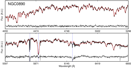
Figure 11: The optical spectra for the template-galaxies (labeled on top-left) with overlaid its best-fitting stellar spectrum (red line) derived with the pPXF approach (Sect. 3.1) along with the residuals. The location of the spectral features masked out during the fitting are marked with blue dotted lines.

Fig. 11 – Continued.

Fig. 11 – Continued.

Fig. 11 – Continued.

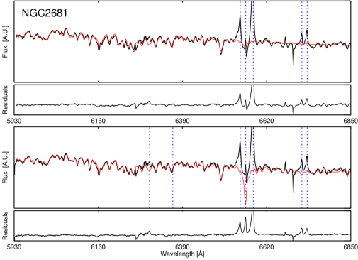
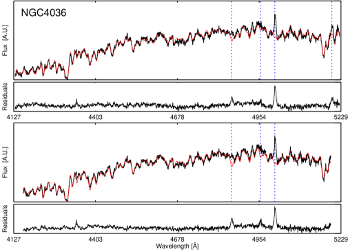
Figure 12: Stellar continuum modelling performed with different methods for those LINERs with questionable pPXF modelling (Sect. 3.1). The red line indicates the modelled stellar spectrum that matches the observed continuum, obtained applying the pPXF (top) and STARLIGHT (bottom) methods (Sect. 3.1). The location of the spectral features masked out during the fitting are marked with blue dashed lines. The spectra are shown with a zoomed view to highlight weak continuum features. Moreover the region redward to $\sim$ 6850 Å is not considered in these plots as dominated by atmospheric absorption. The lower panels show the residuals from the stellar subtraction after the stellar continuum modeling. For all these cases the selected model is STARLIGHT (see also Table LABEL:T_kin).

Fig. 12 – Continued.

Fig. 12 – Continued.

Fig. 12 – Continued.

Table 10: Summary of the values evaluated to prevent overfitting emission lines.

ID	Obs.	Mod.	Comp.	$\varepsilon_{\rm c}$	$\varepsilon$${}^{\rm[O\,I]}$N	$\varepsilon$${}^{\rm[O\,I]}$N+S	$\varepsilon$${}^{\rm[S\,II]}$N	$\varepsilon$${}^{\rm[S\,II]}$N+S	$\varepsilon$HαN(+S)	$\varepsilon$HαN+B(+S)
NGC 0226	CAHA†	O	N + S	0.0143	1.3893	1.5088	—	—	2.3668	—
NGC 0315	[NOT]	M	N + S + B	0.0061	2.9184	1.9224	4.2010	1.9160	5.0966	5.4522
	HST †	S	N + S + B	12.764	—	—	3.6023	2.1042	7.6608	2.2244
NGC 0841	CAHA	S	N	0.0179	1.2525	—	0.7633	—	1.0398	—
NGC 1052	[NOT]	M	N + S	0.0436	5.2044	2.6391	4.8007	1.9587	7.6481	—
	[HST]	M	N + S + B	10.535	7.3194	2.5107	5.6332	2.5163	11.893	5.4754
NGC 2681	CAHA	O	N + S	0.0042	2.6604	2.5589	—	1.4102	2.3355	1.0018
NGC 2787	CAHA	S	N + B	0.0221	1.3256	—	1.0097	—	1.3392	—
	HST ‡	S	N + B	61.142	0.8707	—	0.8906	—	1.7578	1.0298
NGC 3226	CAHA	O	N + S	0.0134	1.3636	1.1753	—	1.7574	2.5608
NGC 3642	[CAHA]	M	N + S + B	0.0163	1.7874	1.7838	3.5604	1.2728	4.4198	4.3211
	[HST] †	S	N + B	24.277	—	—	1.5359	—	8.0335	6.2624
NGC 3718	CAHA	M	N + B	0.0152	1.7210	—	1.0180	—	1.8414	1.4384
NGC 3884	CAHA †	O	N + S	0.0066	1.3960	1.2535	—	—	1.8567	—
NGC 3998	[CAHA]	O	N + S	0.0520	3.9890	2.5499	—	2.4168	3.7271	—
	HST ‡	M	N + B	313.70	1.9269	—	1.1459	—	7.983	3.0695
NGC 4036	CAHA	M	N + S	0.0311	1.1460	1.0271	1.0590	1.0142	1.3522	—
	HST	M	N + B	9.0111	0.9509	—	0.8204	—	2.6777	2.4079
NGC 4143	CAHA	M	N + S	0.0047	2.3230	2.0726	1.7070	1.4728	3.2108	—
	HST ‡	S	N + S + B	45.540	—	1.4536	1.2072	1.1482	2.3801	1.5893
NGC 4203	CAHA	M	N + S + B	0.0099	2.0212	1.3327	1.7502	1.1678	6.0657	2.8283
	[HST]	M	N + S + B	31.058	4.7849	2.1168	4.0582	1.6267	18.517	5.7687
NGC 4278	CAHA	M	N + S	0.0116	2.5285	2.1568	2.2769	1.8593	3.0817	—
	HST ‡	M	N + S + B	6.6675	1.6094	1.4464	1.3310	0.9954	2.3561	1.9355
NGC 4438	[CAHA]	M	N + S	0.0095	2.9692	2.4282	3.7552	1.1571	4.3757	—
NGC 4450	CAHA	M	N + S	0.0284	1.4971	1.1393	1.0932	0.5911	1.3655	—
	HST	M	N + S + B	33.585	2.0183	1.5548	2.4561	1.8462	7.9210	2.7456
NGC 4636	CAHA	S	N + B	0.0088	1.9763	—	1.1856	—	2.2206	1.8684
NGC 4750	CAHA	O	N + S + B	0.0180	1.6476	1.4759	—	1.0711	2.1151	2.3040
NGC 4772	CAHA	S	N	0.0121	1.6562	—	1.8778	—	2.0312	—
NGC 5005	[CAHA]	S	N + S	0.0299	—	2.0176	2.1457	2.4765	3.5698	—
	HST †	S	N + S + B	31.407	—	—	1.9060	1.3951	2.0732	1.1658
NGC 5077	CAHA	S	N + B	0.0202	1.2003	—	0.5672	—	1.5123	0.8314
	HST †	S	N + S + B	20.042	—	—	1.4208	1.2749	1.9169	1.5632

Notes. ‘ID’: object designation as in Table 1. ‘OBS’: origin of the optical data. ‘Mod.’: best-fitting model for emission lines. ‘S’, ‘O’ and ‘M’ stand for models based on [S II] or [O I] or mixed -type. ‘Comp.’: components used to achieve the best-fitting model. ‘N’ and ‘B’  stand for narrow and broad, component, while ‘S’ indicates the second component when present (see Sect. 3.2, for details). The values of the standard deviation calculated in the residual spectra considering a line-free continuum ($\varepsilon_{\rm c}$) and emission lines ($\varepsilon$${}^{\rm[O\,I]}$, $\varepsilon$${}^{\rm[S\,II]}$ and $\varepsilon$^Hα in until of $\varepsilon_{\rm c}$) in the residual spectrum after the fitting, for different components. ^† and ^‡ symbols are as in Table LABEL:T_kin. Square-brackets indicate the data for which the fit of the H$\alpha$-[N II] emission is not well constrained ($\varepsilon$^Hα$>$ 3 $\varepsilon_{\rm c}$).

Appendix B Comments, spectra and images of individual sources

The first part of this appendix is devoted to shortly comment the characteristics of each LINER.

In the second part, we show the HST-image (in the F814W-band if available) from the Hubble Legacy Archive and the spectra analysed in this manuscript for each LINER.
More specifically, we present ‘sharp-divided’ HST images. A sharp-divided image (Márquez et al., 1999, 2003) is obtained by dividing the original image, I, by a filtered version of it, BI, i.e. I / BI. Its result is very similar to that of the unsharp masking technique (which subtracts instead of dividing, i.e. I - BI), but for the former the levels are around unity, which facilitates the comparison among different galaxies. Features departing from axisymmetry, together with those with sizes close to the size of the filter are better seen in the sharp-divided images. In our case, the images are median filtered with the iraf command ‘median’ using a box of 30 pixels. As shown in the figures of this Appendix, the results clearly show asymmetric structures in the centres, that cannot be appreciated in the original images.
We present rest-frame blue and red spectra and the corresponding stellar continuum-model and the Gaussian fits to emission lines profiles after stellar-subtraction. When available, the line-modelling to HST/STIS line profiles is also shown.
The images and spectra are arranged as follows:
Top: HST image, the orientation is North up, East to the left. Overlaid to these HST-images, we mark the slit used to obtain the data analysed in this work and the major axis of rotation (from the HyperLeda database) with continuos and dashed lines, respectively. The white bar shows a linear scale of 100 pc (see also column 3 in Table 1). For the LINERs at z $\geq$ 0.005 (Table 1), we indicate a larger linear scale (either 200, 300 or 400 pc). If available, the line-modelling to HST/STIS line profiles is also shown.
Middle: the 2 lines show the ground-based, rest-frame spectra and their continuum-model for the blue and red ranges. The residuals (i.e. data - model) are also presented. The red line indicates the modelled stellar spectrum that matches the observed stellar continuum (Sect. 3 and Table LABEL:T_kin). The central wavelength of the most relevant spectral features masked-out in the procedure for the stellar continuum modelling (as in Fig. 1) are marked with vertical lines. Specifically, in green and in blue those emission lines considered and excluded for the analysis, respectively.
Bottom: Gaussian fits to emission lines profiles (after stellar continuum subtraction) in both blue (left) and red (right) spectra. We marked with different colours the Gaussian components required to model the emission lines (same colours mark the same kinematic components). These components are named on the top-right and summarised in Table LABEL:T_kin (see also Sect. 3, for details). The red curve shows the total contribution coming from the Gaussian fit. Residuals from the fit are in the small lower-panels in which grey lines indicate the rest frame wavelengths of the emission lines.
For each LINER, the caption include comments about the line profiles in ground-based data and their modelling. We refer to BC14 (and references therein) for similar comments but for emission lines and their fit for HST/STIS spectra.

Finally, the third part of this appendix is devoted to the present position-velocity diagrams (PV curves) for each LINERs.

NGC 0266. This LINER-nucleus is hosted by a spiral galaxy with a well studied bar (Font et al., 2017). Garrido et al. (2005), GHASP survey, found that the rotation curve exhibits a strong velocity gradient in the inner $\sim$ 5″ (i.e. $\sim$1.6 kpc), reaching a maximuum rotational velocity of 363 kms^-1 at a larger distance (26 kpc). The CAHA spectroscopic data also show evidence for rotation (Fig. 35) but with lower rotational velocity than what found by Garrido et al. (2005) since our PA is not placed along the major axis (Fig. 13). We also report for the first time the detection of a kinematic component likely associate to a possible outflow. HFS97 reported a BLR component with a FWHM of 1350 km s^-1, but we did not. The red spectrum of this LINER does not cover the [S II] doublet (Sect. 3.2) and the blue spectra has a low S/N. The NaD absorption has been modelled with two kinematic components (Fig. 3). The narrow component shares the same velocity dispersion with the same component of the ionised gas, but the velocities of the two ISM-phases are somewhat different (Table LABEL:T_kin). The second, and broader one, is different than the same component of the ionised gas, though both have blueshifted velocities (Table LABEL:T_kin).

NGC 0315. The nucleus of this elliptical galaxy shows an unresolved source of ionised gas on top of a dusty disc of $\sim$ 200 pc visible in the HST image (Masegosa et al., 2011). Two-sided, well-resolved radio jets are associated to the X-ray jet at PA = -49^∘ (Nagar, Falcke & Wilson, 2005; Kharb et al., 2012). Therefore this jet-structure is not aligned with the possible outflow found in our spectroscopic study (Table LABEL:class_sum). Such an outflow would have a complex ionization structure as the properties of low and high ionization lines are different (Table LABEL:T_kin). The broad H$\alpha$ component is detected in both our ground- and space-based spectroscopy and in previous works (Table LABEL:T_FWHM). Unfortunately, such component is not well constrained in our fit with ALFOSC/NOT data (Table LABEL:T_rms). Part of the discrepancy of measurements at different epochs may be due to AGN variability on scales of years (as reported by Younes et al. 2011; Hernández-García et al. 2014). The 2D rotation is very perturbed (Fig. 35). The neutral gas kinematics is very different from that of the ionised gas with redshifted velocity and with a velocity dispersion larger (smaller) than that of the narrow (second) component in emission lines. The latter consideration reflects the general behaviour of the neutral gas in our sample of LINERs (Sect. 3.3).

NGC 0841. It is classified as a grand design nuclear spiral with a spiral dust lane down to the centre by González Delgado et al. (2008). Rotation is clearly detected (though with some distortion, Fig. 35) even if our slit is not aligned with the major axis (Fig. 15). A BLR component is not needed to model, in our ground-based spectrum, the H$\alpha$ line profile (which is not blended with [N II]), though previously reported by HFS97. The NaD doublet seems to originate in a neutral gas rotating disc whose kinematics is rather similar to that of the ionised gas (velocity dispersions are the same within uncertainties, Tables LABEL:T_kin and 5).

NGC 1052. An elliptical galaxy with large scale dusty structures harbors the prototypical LINER nucleus. It is an X-ray absorbed source with little optical obscuration and broad lines in polarized light (Barth, Filippenko & Moran, 1999) indicating a peculiar absorbing geometry (Burtscher et al., 2016). Space-and ground-based red optical spectra are remarkably similar (with a severe H$\alpha$-[N II] blend), except for [S II]. Onori et al. (2017) modelled the [N II] emission an HST/FOS spectrum (R = 2800) with one Gaussian though with rather large FWHM, i.e. 682 km s^-1 that may indicate the presence of unresolved outflow components. The BLR component in their analysis is of $\sim$ 2200 km s^-1, a slightly larger value is found considering the near-IR He I$\lambda$1.083$\mu$m line i.e. $\sim$ 2400 km s^-1. The broad H$\alpha$ component was also detected by BC14 and C15, in fair agreement (Table LABEL:T_FWHM). We found evidence for the BLR only in HST/STIS spectra. This could be partially due to a less reliable fit to the H$\alpha$ emission line in ground- and space-based datasets (Table LABEL:T_rms). Second components in Oxygen and Hydrogen lines are interpreted as a possible outflow (Table LABEL:class_sum) as already suggested in previous works (Pogge et al., 2000; Walsh et al., 2008; Dopita et al., 2015; Sugai et al., 2005). [S II] behaves otherwise than [O I] in both ground- and space-based spectroscopy (Tables LABEL:T_kin and LABEL:class_sum). The neutral gas probed via NaD shares the same kinematics with the narrow component of the [O I] (Tables LABEL:T_kin and 5).

NGC 2681. It is a S0 galaxy with large-scale spiral dust lanes (Masegosa et al., 2011). The second component fitted to the emission lines is relatively narrow (209 $\pm$ 12 km s^-1) and blueshifted (-180 $\pm$ 8 km s^-1). This might indicate a complex nuclear rotation pattern, in fair agreement with the complicated and multi-component structure already reported via optical and near-IR imaging by Dullo, Martínez-Lombilla & Knapen (2016) and Laurikainen, Salo & Buta (2005). Interestingly, both star-formation and AGN optical BPT line ratios are observed by the nucleus with the first increasingly significant when the aperture size is increased (Dullo, Martínez-Lombilla & Knapen, 2016).

NGC 2787. The most noticeable feature of this lenticular galaxy is a set of concentric elliptical dust rings (Masegosa et al., 2011). There is a good match between the modelling of ground- and space-based data, in terms of the adopted model and number of components. The FWHM of the BLR components are nevertheless quite different (Table LABEL:T_FWHM) being $\sim$ 1000 km s^-1 lower in ground-based data than that from HST/STIS spectroscopy in present and previous works. This could be due to short-term variability (Hernández-García et al., 2014). Based on integral field spectroscopic data, Brum et al. (2017) probed a pure rotation velocity field with high projected amplitude ($\sim$ 250 km s^-1) which is also partially captured by CAHA observations (Fig. 35). Additionally they found a mild AGN outflow and nuclear bar (see also Erwin et al. 2003). We did not find any sign of complex kinematics associated to these features probably due to a different slit orientation and the contribution from the bar and a putative outflow. The component used to model the neutral gas NaD absorption shares similar kinematics to that of the narrow component of the ionised gas (Tables LABEL:T_kin and 5). However, the doublet is affected by absorption telluric lines making the line modelling uncertain (Fig. 3), and avoiding the detection of a putative blueshifted second component.

NGC 3226. This elliptical galaxy is characterised by a bright and compact nucleus in a dusty environment. The kinematics of the second component indicate the presence of a possible outflow (at a velocity of 155 $\pm$ 21 km s^-1) consistent with the outflow-like structure emerging from the nucleus seen in HST images (Masegosa et al., 2011). Though evidence for the presence of an AGN has been found via X-ray by Capetti & Balmaverde (2006), the optical H$\alpha$ line-profile modelling does not require any BLR-originated component. The NaD doublet was modelled with a single kinematic component (Fig. 3) found at the systemic velocity (2 $\pm$ 2 km s^-1). Its velocity dispersion (212 $\pm$ 42 km s^-1, Table 5) agrees within the uncertainties with that of the narrow component of the ionised gas (185 $\pm$ 20 km s^-1Table LABEL:T_kin). However, as for NGC 2787, the blue wing of the absorption doublet is affected by the residual of skyline subtraction and telluric absorption (Fig. 3).

NGC 3642. A strong point source is surrounded by some diffuse circumnuclear H$\alpha$ emission in this LINER (Pogge et al., 2000). It is hosted by a spiral galaxy with large-scale dusty structures and several H II regions (Chiaberge, Capetti & Macchetto, 2005). The second kinematic component is classified as a candidate for a possible outflow, this is probably a consequence of our conservative limits. Indeed, the kinematical properties of this component (V = -335 $\pm$ 67 km s^-1 and $\sigma$ = 300 $\pm$ 60 km s^-1) are most likely not due to the rotation which shows a small amplitude ($<$ 100 km s^-1, Fig. 35). The BLR detection is confirmed with both ground- and space-based optical spectroscopy (Table LABEL:T_FWHM), although the H$\alpha$-fit is less reliable (Table LABEL:T_rms). Only some X-ray properties of this LINER in ROSAT observations are present (Komossa, Böhringer & Huchra 1999 and references therein). The stellar subtraction leaves some residuals that can be interpreted as resonant NaD emission. Unfortunately, the low S/N in this wavelength region makes highly questionable the detection of such peculiar emission.

NGC 3718. This spiral galaxy has a prominent dust lane, which runs across the entire stellar bulge, and a warped molecular and atomic gas disc (Sparke et al., 2009; Krips et al., 2005). It also shows signs of a past interaction (probably with NGC 3729, Markakis et al. 2015). The elongated structures seen in the HST images and e-MERLIN data are indicative of a small-scale bipolar jets or outflows. As for the case of NGC 0315, different measurements of the BLR components (Table LABEL:T_FWHM) could be due to AGN variability on scales of years (Younes et al., 2011). The region of NaD is strongly affected by telluric absorption compromising the possibility to infer the neutral gas kinematics.

NGC 3884. The optical emission line profiles observed in this spiral galaxy have been modelled with two kinematical components. The narrow component is interpreted as rotation which has a small amplitude as seen in the corresponding PV-curve (Fig. 35). The second component is rather broad and blueshifted, and it is interpreted as a possible outflow (Table LABEL:class_sum). As for the case of NGC 3642, the detection of a resonant NaD emission is uncertain.

NGC 3998. This S0 galaxy has a disc-like weak emission with a diameter of $\sim$ 100 pc surrounding a compact nucleus and little indication of dust in the nuclear region (Pogge et al., 2000; Masegosa et al., 2011). The 2D gas kinematics is disc dominated by disc rotation, classified as a near-oblate, face-on fast rotator by Boardman et al. (2016). Some anisotropies and signs of warps are found at large galactocentric distance likely related to a past interaction (Boardman et al., 2017). The disc kinematics is not fully captured by our ground-based spectroscopy likely due to the slit orientation with respect to the major axis (Fig. 23). X-ray spectroscopy at 0.1-100 keV data provides a strong indication for an AGN origin of the LINER activity in this galaxy (Pellegrini et al., 2000). The nucleus is a low-power radio AGN with a kpc-size one-sided jet and S-shaped lobes with a total extent of about 20 kpc (Frank et al., 2016). We do find evidence of a BLR-originated component only in HST/STIS spectra; this could be partially due to a not fully reliable fit to the H$\alpha$ emission line in ground-based data (Table LABEL:T_rms). Components of intermediate width in ground-based spectroscopy are interpreted as a possible outflow (Table LABEL:class_sum). Broad forbidden lines are also found in the space HST/STIS spectrum but their fit is rather uncertain. The NaD doublet has been modelled with a single kinematic component (Fig. 3) found at the systemic velocity but with rather high velocity dispersion ($\sigma$ = 292 $\pm$ 58 km s^-1), intermediate between those of the narrow and second components of the emission lines (Table LABEL:T_kin). Similarly to the cases of NGC 2787 and NGC 3226, the doublet is affected by skylines and telluric absorption making the line modelling less reliable (Fig. 3).

NGC 4036. This E-S0 galaxy is characterised by a well-identified nucleus and a complex filamentary and clumpy structure with several filaments (Pogge et al., 2000; Masegosa et al., 2011; Walsh et al., 2008). Both narrow and second components of emission lines are identified with rotation (Sect. 5.2 and Table LABEL:class_sum). However, the second broader component could be associated to the complex H$\alpha$ emission structure present in the inner 3″. 2D spectroscopic data at higher spectral and spatial resolution are needed to study this feature in detail. A broad component is not required to fit the H$\alpha$-profile in our ground-based spectra in contrast to what was found by HFS97. Such a broad component is essential to model H$\alpha$ in the HST/STIS spectrum.

NGC 4143. For this E-S0 galaxy, we modelled the forbidden line profiles with two kinematic components in both ground- and space-based spectra. However, only the second component of Oxygen lines in ground-based data, indicates the possible presence of an outflow. A broad component is needed for modelling the H$\alpha$ line only in HST/STIS spectra. The FWHM of this component is larger than 1000 km s^-1 than that measured by HFS97 based on [S II] as reference; a much smaller difference is found when using [O I] as reference in BC14 (Table LABEL:T_kin).

NGC 4203. It is a nearly face-on SAB with a large-scale dusty structures (Chiaberge, Capetti & Macchetto, 2005). This galaxy is surrounded by a very large, low-column-density and distorted H I disc and a disrupted companion dwarf galaxy is present at the east of the galaxy (Yıldız et al., 2015). The nucleus is variable in the optical (Devereux, 2011), UV (Maoz et al., 2005), and radio (Nagar et al., 2002). A possible explanation for the double-peaked broad H$\alpha$ emission line (Ho, Filippenko & Sargent, 1997a; Shields et al., 2007; Balmaverde & Capetti, 2014) is the presence of an inflow associated with the accretion disc, since the former, presumably, fuels the latter (Devereux, 2011). This would be consistent with the presence of the possible inflow-components found in both ground- and space-based data. A component coming from a weak outflow was also detected in [S II] in ground-based data. However, the broad H$\alpha$ is contaminating these line profiles, therefore their interpretation is rather uncertain.
The fit to the H$\alpha$ emission line in both ground- and space-based data is not reliable (Table LABEL:T_rms) since a more elaborate physical modelling would be needed to fit the very broad and double-peaked emission line profile (likely originated in the outer parts of the accretion disc surrounding the SMBH, e.g. Storchi-Bergmann et al. 2017).

NGC 4278. It is a relatively isolated elliptical galaxy with complex and irregular dust structure in its core with knots and filaments and a two-sided pc-scale jet (Pellegrini et al., 2012). The narrow components are interpreted as rotation in agreement with Sarzi et al. (2006) and Morganti et al. (2006) who already found a kinematical structure typical of an extended and regular disc. The second component is interpreted as a possible inflow and could be consistent with a small accretion region present at the centre. A more detailed, possibly 2D-IFS, study of the interplay between the ISM and nuclear activity is needed to confirm this scenario. A broad H$\alpha$ component is extracted from the complicated blend observed in HST/STIS data, only.

NGC 4438. This spiral galaxy has a disturbed morphology with strong dust lanes and a ring-like structure (Masegosa et al., 2011). The latter may be a consequence of environmental effects or the close interaction with M86 and/or NGC 4435 (Cortese et al., 2010). Both narrow and second components are interpreted as rotation (as for the case of NGC 2681) but the 2D rotation curve has a very low amplitude and is perturbed (Fig. 35). The second (broader) components ($\sigma$ $\sim$ 200 km s^-1, Table LABEL:T_kin) could be either related to its complex nuclear morphology or related to the H$\alpha$ outflow-like structure in Masegosa et al. (2011). We did not find evidence for a BLR component but our modelling of H$\alpha$ is not fully reliable (Table LABEL:T_rms). Overall, the peculiar properties of NGC 4438 make it an ideal target for IFS observations.

NGC 4450. Brum et al. (2017) found a clear rotating disc pattern with the line of nodes oriented along the North-South direction with some deviations. The flat and low amplitude rotation curve presented in Fig. 35 partially disagrees with that obtained by Cortés, Kenney & Hardy (2015) probably due to difference in slit orientations (Fig. 29). The same authors interpreted the perturbation of the rotation curve either as due to non-circular motions or related to an external gas acquisition or a minor merger event (see also Coccato et al. 2013). All this could be in agreement with the complex outflow/inflow scenario suggested by the second components of the forbidden lines (Table LABEL:class_sum); but spatially resolved data at higher spectral resolution are needed to confirm this hypothesis. A double-peaked broad H$\alpha$ line profile (interpreted as the signature of the outer parts of a relativistic accretion disc) has been reported by Ho et al. (2000). Interestingly, this feature is completely absent in our ground-based spectroscopic data being only evident in HST/STIS data.

NGC 4636. It is one of the most well-known nearby elliptical galaxies. It has a central compact source and a very faint ring-like structure (Masegosa et al., 2011). The prominent emission towards the North with a clear outflow-like morphology (Masegosa et al., 2011) is consistent with X-ray observations (O’Sullivan, Vrtilek & Kempner, 2005). These X-ray data confirm the presence of a cavity and a plume that appear to be the product of past AGN activity (AGN outbursts), with the AGN being quiescent at present. This could explain the relatively low FWHM of the broad H$\alpha$ component (considering our sample). Unfortunately, the outflow-like structure is not fully captured in our CAHA spectroscopy (probably due to to slit orientation).

NGC 4750. This spiral galaxy has a very bright nucleus with some arc or shell-like structures (Mason et al., 2015). The position-velocity curve shows some clear asymmetries at large radii (Fig. 35). The presence of a faint blue wing in Oxygen lines is interpreted as possibly being originated by an outflow (Tables LABEL:T_kin and LABEL:class_sum). The measurement of the FWHM of the BLR-component is in fair agreement with that reported by HFS97. Blueward of the NaD, the spectrum is rather noisy due to some residual telluric absorption. Despite this, we were able to model the weak doublet feature with one kinematical component (Fig. 3); it has a completely different kinematics with respect to the ionised gas (Tables LABEL:T_kin and 5), with a low velocity dispersion and a rather large blueshifted velocity.

NGC 4772. The optical emission line profiles of this spiral galaxy (known as ‘eye galaxy’) are well modelled with only one kinematic component. The velocity is rest frame, the velocity dispersion is the largest among our measurements for the narrow component (i.e. 249 $\pm$ 12 km s^-1). Such broadening is likely due to the chaotic kinematics (i.e. a superposition of multiple components) present in the individual spectra in our nuclear aperture. This could be consistent with the results obtained by Haynes et al. (2000b), who found that the stars and the ionised gas in the centre of this galaxy are counter-rotating (often taken as an indication of a merger). Many knots are observed inside the slit we used to obtain the present ground-based data; preventing a reliable position-velocity distribution.

NGC 5005. The distinguish features of this weakly barred spiral galaxy are the strong dust lane crossing the galaxy from East to West (offset from the nucleus), the fan-shaped filaments, the compact nuclear clumps and its obscured nucleus (Pogge et al., 2000). The presence of a weak AGN is confirmed by the detection of a compact hard X-ray source (González-Martín et al., 2006) which is variable on scales of months (Younes et al., 2011). The second component in the CAHA spectrum is interpret as a possible outflow. In the HST-spectrum a second component is also present and is interpreted as a candidate outflow. This component is at the same velocity of the outflow seen in ground-based data ($\sim$ 110 km s^-1), the velocity dispersion is slightly lower (308 vs. 446 km s^-1) but consistent within uncertainties. These results are consistent with the interpretation of the H₂$\lambda$2.122$\mu$m, [Fe II]$\lambda$1.644$\mu$m and Br$\gamma$$\lambda$2.166$\mu$m near-IR flux measurements by Bendo & Joseph (2004). The BLR component is only detected in the HST/STIS spectroscopic data, possibly due to a less reliable fit to the H$\alpha$ emission line in ground-based data (Table LABEL:T_rms).

NGC 5077. This elliptical galaxy has a compact unresolved source in the nucleus and dust lanes on top of a smooth gas distribution. The observed position-velocity curve (Fig. 35) and the narrow component in the the CAHA/TWIN spectra are consistent with gas in regular rotation around the galaxy centre (as seen also by de Francesco, Capetti & Marconi 2008). A second component that may be produced by an outflow is present only in the HST/STIS spectrum (Table LABEL:class_sum). A broad component is required for modelling the H$\alpha$ line profile in both ground- and space-based spectroscopic data (Table LABEL:T_FWHM).

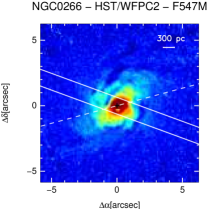
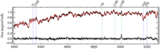
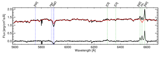
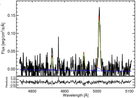
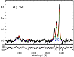
Figure 13: First row: sharp divided HST image. The two continuous white lines represent the slit used in our ground-based spectroscopy. The PA of the major axis is marked with a dashed line. When an HST/STIS spectrum is available, the line modelling is shown. Second and third rows: rest-frame ground-based blue and red spectra, respectively; the red line corresponds to the continuum reproducing the stellar population, the vertical lines mark the most relevant spectral features masked out before the continuum fitting. Forth row: Gaussian fit to the stellar population subtracted spectra in the H$\beta$ (left) and H$\alpha$ (right) regions. We marked with different colours the components, named on the top-right, required to model the emission lines. The red curve shows the total contribution from the fit. Residuals from the fit are in the lower-panels in which grey lines mark the rest frame wavelengths of the spectral features.
NGC 0266: The H$\alpha$-[NII] lines are unblended in the observed spectrum. An additional second component is evident in the narrow lines only after starlight subtraction. The single-component model of [O I] has lower residuals than the double Gaussians one (Table LABEL:T_rms). However, such single component would have a width of $\sim$ 750 km s^-1 which is unrealistically large. We did not find strong evidence of a BLR component in contrast of what found by HFS97.

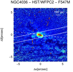
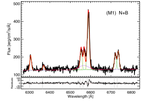
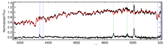
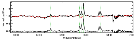
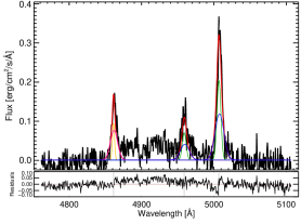
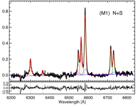
Figure 24: (General description as in Fig. 13.) NGC 4036: the presence of wings in all emission lines suggests that a second component, whose inclusion produces a small improvement in the modelling of [O I] (Table Table LABEL:T_rms), is true and not an artifact. [S II] and [O I] line profiles are quite different. The second component is less evident in [S II] (wings are almost absent). We did not find evidence of the broad component in our ground-based data, whereas it is however rather faint in the Palomar spectrum (HFS97). The evidence for such a broad component in H$\alpha$ seems clear in the HST/STIS spectrum.

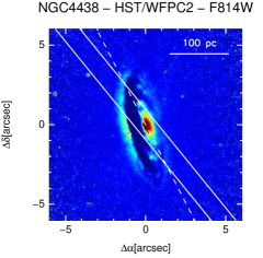
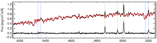
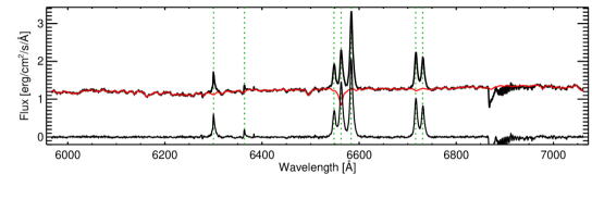
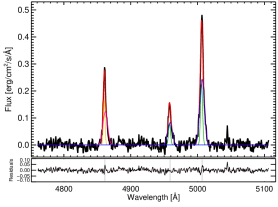
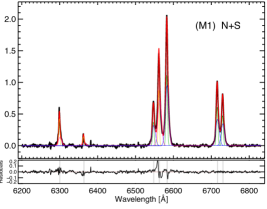
Figure 28: (General description as in Fig. 13.) NGC 4438: all emission lines are relatively narrow. However, blue and red wings are detected in both [O I] and [S II] lines. The broad component is not required for modeling the H$\alpha$ emission contrary to what was found by HFS97 in the analysis of the Palomar spectrum (note that their broad component was the weakest among their detections).

Fig. 35 – continues.

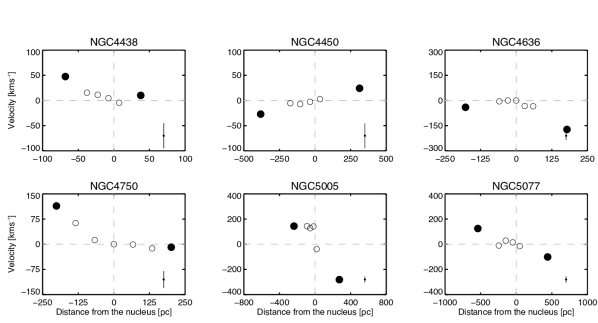
Figure 35: Position-velocity diagram for all the LINERs in the sample except NGC 4772. For this LINER the velocity distribution is very chaotic with multiple kinematic components already in the innermost regions, preventing to constrain any putative rotation pattern. The empty circles mark those data-points obtained considering the peak velocity of the most intense emission line (generally [N II]$\lambda$6584) in the individual spectra corresponding to the nuclear extraction. As a reference, we show the velocities corresponding to the individual spectra at larger distances from the center. Positions and velocities for a given galaxy are referred to that of the central spectrum in its nuclear extraction (the lines tracing the origin of coordinates are plotted as pink, dashed lines. At the bottom-right of each panel we show an error-bar representative for all the measurements.

References

- Allen et al. (2008) Allen M. G., Groves B. A., Dopita M. A., Sutherland R. S., Kewley L. J., 2008, \apjs, 178, 20
- Annibali et al. (2010) Annibali F., Bressan A., Rampazzo R., Zeilinger W. W., Vega O., Panuzzo P., 2010, \aap, 519, A40
- Arribas et al. (2014) Arribas S., Colina L., Bellocchi E., Maiolino R., Villar-Martín M., 2014, \aap, 568, A14
- Bae & Woo (2016) Bae H.-J., Woo J.-H., 2016, \apj, 828, 97
- Baldwin, Phillips & Terlevich (1981) Baldwin J. A., Phillips M. M., Terlevich R., 1981, \pasp, 93, 5
- Balmaverde & Capetti (2014) Balmaverde B., Capetti A., 2014, \aap, 563, A119
- Balmaverde et al. (2016) Balmaverde B., Capetti A., Moisio D., Baldi R. D., Marconi A., 2016, \aap, 586, A48
- Barth, Filippenko & Moran (1999) Barth A. J., Filippenko A. V., Moran E. C., 1999, \apjl, 515, L61
- Bendo & Joseph (2004) Bendo G. J., Joseph R. D., 2004, \aj, 127, 3338
- Binette et al. (1994) Binette L., Magris C. G., Stasińska G., Bruzual A. G., 1994, \aap, 292, 13
- Boardman et al. (2017) Boardman N. F. et al., 2017, \mnras, 471, 4005
- Boardman et al. (2016) Boardman N. F. et al., 2016, \mnras, 460, 3029
- Brum et al. (2017) Brum C., Riffel R. A., Storchi-Bergmann T., Robinson A., Schnorr Müller A., Lena D., 2017, \mnras, 469, 3405
- Bruzual & Charlot (2003) Bruzual G., Charlot S., 2003, \mnras, 344, 1000
- Burtscher et al. (2016) Burtscher L. et al., 2016, \aap, 586, A28
- Capetti & Balmaverde (2006) Capetti A., Balmaverde B., 2006, \aap, 453, 27
- Cappellari (2017) Cappellari M., 2017, \mnras, 466, 798
- Cappellari & Emsellem (2004) Cappellari M., Emsellem E., 2004, \pasp, 116, 138
- Cappellari et al. (2007) Cappellari M. et al., 2007, \mnras, 379, 418
- Cappellari et al. (2011) Cappellari M. et al., 2011, \mnras, 413, 813
- Cardelli, Clayton & Mathis (1989) Cardelli J. A., Clayton G. C., Mathis J. S., 1989, \apj, 345, 245
- Carniani et al. (2015) Carniani S. et al., 2015, \aap, 580, A102
- Cazzoli et al. (2014) Cazzoli S., Arribas S., Colina L., Piqueras-López J., Bellocchi E., Emonts B., Maiolino R., 2014, \aap, 569, A14
- Cazzoli et al. (2016) Cazzoli S., Arribas S., Maiolino R., Colina L., 2016, \aap, 590, A125
- Chiaberge, Capetti & Macchetto (2005) Chiaberge M., Capetti A., Macchetto F. D., 2005, \apj, 625, 716
- Chisholm et al. (2016) Chisholm J., Tremonti C. A., Leitherer C., Chen Y., Wofford A., 2016, \mnras, 457, 3133
- Cid Fernandes et al. (2005) Cid Fernandes R., Mateus A., Sodré L., Stasińska G., Gomes J. M., 2005, \mnras, 358, 363
- Cid Fernandes et al. (2009) Cid Fernandes R. et al., 2009, in Revista Mexicana de Astronomia y Astrofisica Conference Series, Vol. 35, Revista Mexicana de Astronomia y Astrofisica Conference Series, pp. 127–132
- Cid Fernandes et al. (2011) Cid Fernandes R., Stasińska G., Mateus A., Vale Asari N., 2011, \mnras, 413, 1687
- Coccato et al. (2013) Coccato L., Morelli L., Pizzella A., Corsini E. M., Buson L. M., Dalla Bontà E., 2013, \aap, 549, A3
- Coil et al. (2011) Coil A. L., Weiner B. J., Holz D. E., Cooper M. C., Yan R., Aird J., 2011, \apj, 743, 46
- Constantin et al. (2015) Constantin A., Shields J. C., Ho L. C., Barth A. J., Filippenko A. V., Castillo C. A., 2015, \apj, 814, 149
- Cortés, Kenney & Hardy (2015) Cortés J. R., Kenney J. D. P., Hardy E., 2015, \apjs, 216, 9
- Cortese et al. (2010) Cortese L. et al., 2010, \aap, 518, L63
- Davis et al. (2012) Davis T. A. et al., 2012, \mnras, 426, 1574
- de Francesco, Capetti & Marconi (2008) de Francesco G., Capetti A., Marconi A., 2008, \aap, 479, 355
- Devereux (2011) Devereux N., 2011, \apj, 743, 83
- Dopita et al. (2015) Dopita M. A. et al., 2015, \apj, 801, 42
- Dopita et al. (1996) Dopita M. A., Koratkar A. P., Evans I. N., Allen M., Bicknell G. V., Sutherland R. S., Hawley J. F., Sadler E., 1996, in Astronomical Society of the Pacific Conference Series, Vol. 103, The Physics of Liners in View of Recent Observations, Eracleous M., Koratkar A., Leitherer C., Ho L., eds., p. 44
- Draine (2011) Draine B. T., 2011, Physics of the Interstellar and Intergalactic Medium
- Dudik, Satyapal & Marcu (2009) Dudik R. P., Satyapal S., Marcu D., 2009, \apj, 691, 1501
- Dullo, Martínez-Lombilla & Knapen (2016) Dullo B. T., Martínez-Lombilla C., Knapen J. H., 2016, \mnras, 462, 3800
- Elitzur, Ho & Trump (2014) Elitzur M., Ho L. C., Trump J. R., 2014, \mnras, 438, 3340
- Elitzur & Shlosman (2006) Elitzur M., Shlosman I., 2006, \apjl, 648, L101
- Epinat et al. (2010) Epinat B., Amram P., Balkowski C., Marcelin M., 2010, \mnras, 401, 2113
- Eracleous & Halpern (2001) Eracleous M., Halpern J. P., 2001, \apj, 554, 240
- Erwin et al. (2003) Erwin P., Beltrán J. C. V., Graham A. W., Beckman J. E., 2003, \apj, 597, 929
- Filippenko & Sargent (1985) Filippenko A. V., Sargent W. L. W., 1985, \apjs, 57, 503
- Filippenko & Terlevich (1992) Filippenko A. V., Terlevich R., 1992, \apjl, 397, L79
- Font et al. (2017) Font J. et al., 2017, \apj, 835, 279
- Frank et al. (2016) Frank B. S., Morganti R., Oosterloo T., Nyland K., Serra P., 2016, \aap, 592, A94
- Ganda et al. (2006) Ganda K., Falcon-Barroso J., Peletier R. F., Cappellari M., Emsellem E., McDermid R. M., de Zeeuw P. T., Carollo C. M., 2006, \mnras, 367, 46
- Garrido et al. (2005) Garrido O., Marcelin M., Amram P., Balkowski C., Gach J. L., Boulesteix J., 2005, \mnras, 362, 127
- González Delgado et al. (2008) González Delgado R. M., Pérez E., Cid Fernandes R., Schmitt H., 2008, \aj, 135, 747
- González-Martín et al. (2017) González-Martín O. et al., 2017, \apj, 841, 37
- González-Martín et al. (2009) González-Martín O., Masegosa J., Márquez I., Guainazzi M., Jiménez-Bailón E., 2009, \aap, 506, 1107
- González-Martín et al. (2006) González-Martín O., Masegosa J., Márquez I., Guerrero M. A., Dultzin-Hacyan D., 2006, \aap, 460, 45
- Groves, Dopita & Sutherland (2004) Groves B. A., Dopita M. A., Sutherland R. S., 2004, \apjs, 153, 75
- Harrison et al. (2014) Harrison C. M., Alexander D. M., Mullaney J. R., Swinbank A. M., 2014, \mnras, 441, 3306
- Harrison et al. (2012) Harrison C. M. et al., 2012, \mnras, 426, 1073
- Haynes et al. (2000a) Haynes M. P., Jore K. P., Barrett E. A., Broeils A. H., Murray B. M., 2000a, \aj, 120, 703
- Haynes et al. (2000b) Haynes M. P., Jore K. P., Barrett E. A., Broeils A. H., Murray B. M., 2000b, \aj, 120, 703
- Heckman (1980) Heckman T. M., 1980, \aap, 87, 152
- Heckman et al. (2000) Heckman T. M., Lehnert M. D., Strickland D. K., Armus L., 2000, \apjs, 129, 493
- Hernández-García et al. (2014) Hernández-García L., González-Martín O., Masegosa J., Márquez I., 2014, \aap, 569, A26
- Hernández-García et al. (2016) Hernández-García L., Masegosa J., González-Martín O., Márquez I., Perea J., 2016, \apj, 824, 7
- Ho et al. (2014) Ho I.-T. et al., 2014, \mnras, 444, 3894
- Ho (2008) Ho L. C., 2008, \araa, 46, 475
- Ho, Filippenko & Sargent (1997a) Ho L. C., Filippenko A. V., Sargent W. L. W., 1997a, \apjs, 112, 315
- Ho, Filippenko & Sargent (1997b) Ho L. C., Filippenko A. V., Sargent W. L. W., 1997b, \apj, 487, 568
- Ho, Filippenko & Sargent (2003) Ho L. C., Filippenko A. V., Sargent W. L. W., 2003, \apj, 583, 159
- Ho et al. (2000) Ho L. C., Rudnick G., Rix H.-W., Shields J. C., McIntosh D. H., Filippenko A. V., Sargent W. L. W., Eracleous M., 2000, \apj, 541, 120
- Hughes et al. (2003) Hughes M. A. et al., 2003, \aj, 126, 742
- Jacoby, Hunter & Christian (1984) Jacoby G. H., Hunter D. A., Christian C. A., 1984, \apjs, 56, 257
- Kauffmann et al. (2003) Kauffmann G. et al., 2003, \mnras, 346, 1055
- Kehrig et al. (2012) Kehrig C. et al., 2012, \aap, 540, A11
- Kewley et al. (2006) Kewley L. J., Groves B., Kauffmann G., Heckman T., 2006, \mnras, 372, 961
- Kharb et al. (2012) Kharb P., O’Dea C. P., Tilak A., Baum S. A., Haynes E., Noel-Storr J., Fallon C., Christiansen K., 2012, \apj, 754, 1
- King & Pounds (2015) King A., Pounds K., 2015, \araa, 53, 115
- Komossa, Böhringer & Huchra (1999) Komossa S., Böhringer H., Huchra J. P., 1999, \aap, 349, 88
- Krips et al. (2005) Krips M. et al., 2005, \aap, 442, 479
- Krug, Rupke & Veilleux (2010) Krug H. B., Rupke D. S. N., Veilleux S., 2010, \apj, 708, 1145
- Kuo et al. (2008) Kuo C.-Y., Lim J., Tang Y.-W., Ho P. T. P., 2008, \apj, 679, 1047
- Laurikainen, Salo & Buta (2005) Laurikainen E., Salo H., Buta R., 2005, \mnras, 362, 1319
- Maiolino et al. (2017) Maiolino R. et al., 2017, \nat, 544, 202
- Maoz et al. (2005) Maoz D., Nagar N. M., Falcke H., Wilson A. S., 2005, \apj, 625, 699
- Markakis et al. (2015) Markakis K. et al., 2015, \aap, 580, A11
- Markwardt (2009) Markwardt C. B., 2009, in Astronomical Society of the Pacific Conference Series, Vol. 411, Astronomical Data Analysis Software and Systems XVIII, Bohlender D. A., Durand D., Dowler P., eds., p. 251
- Márquez et al. (1999) Márquez I. et al., 1999, \aaps, 140, 1
- Márquez et al. (2003) Márquez I., Masegosa J., Durret F., González Delgado R. M., Moles M., Maza J., Pérez E., Roth M., 2003, \aap, 409, 459
- Martin (2005) Martin C. L., 2005, \apj, 621, 227
- Martínez et al. (2008) Martínez M. A., del Olmo A., Coziol R., Focardi P., 2008, \apjl, 678, L9
- Masegosa et al. (2011) Masegosa J., Márquez I., Ramirez A., González-Martín O., 2011, \aap, 527, A23
- Mason et al. (2015) Mason R. E. et al., 2015, \apjs, 217, 13
- Morganti et al. (2006) Morganti R. et al., 2006, \mnras, 371, 157
- Nagar, Falcke & Wilson (2005) Nagar N. M., Falcke H., Wilson A. S., 2005, \aap, 435, 521
- Nagar et al. (2002) Nagar N. M., Falcke H., Wilson A. S., Ulvestad J. S., 2002, \aap, 392, 53
- Netzer (2015) Netzer H., 2015, \araa, 53, 365
- Onori et al. (2017) Onori F. et al., 2017, \mnras, 468, L97
- Osterbrock (1989) Osterbrock D. E., 1989, Astrophysics of gaseous nebulae and active galactic nuclei
- Osterbrock & Ferland (2006) Osterbrock D. E., Ferland G. J., 2006, Astrophysics of gaseous nebulae and active galactic nuclei
- O’Sullivan, Vrtilek & Kempner (2005) O’Sullivan E., Vrtilek J. M., Kempner J. C., 2005, \apjl, 624, L77
- Padovani et al. (2017) Padovani P. et al., 2017, \aapr, 25, 2
- Pellegrini et al. (2000) Pellegrini S., Cappi M., Bassani L., della Ceca R., Palumbo G. G. C., 2000, \aap, 360, 878
- Pellegrini et al. (2012) Pellegrini S., Wang J., Fabbiano G., Kim D.-W., Brassington N. J., Gallagher J. S., Trinchieri G., Zezas A., 2012, \apj, 758, 94
- Pérez-Montero & Contini (2009) Pérez-Montero E., Contini T., 2009, \mnras, 398, 949
- Pogge et al. (2000) Pogge R. W., Maoz D., Ho L. C., Eracleous M., 2000, \apj, 532, 323
- Pović et al. (2016) Pović M., Márquez I., Netzer H., Masegosa J., Nordon R., Pérez E., Schoenell W., 2016, \mnras, 462, 2878
- Riffel et al. (2015) Riffel R. et al., 2015, \mnras, 450, 3069
- Rubin et al. (2012) Rubin K. H. R., Prochaska J. X., Koo D. C., Phillips A. C., 2012, \apjl, 747, L26
- Rupke, Veilleux & Sanders (2005a) Rupke D. S., Veilleux S., Sanders D. B., 2005a, \apj, 632, 751
- Rupke, Veilleux & Sanders (2005b) Rupke D. S., Veilleux S., Sanders D. B., 2005b, \apjs, 160, 87
- Rupke, Veilleux & Sanders (2005c) Rupke D. S., Veilleux S., Sanders D. B., 2005c, \apjs, 160, 115
- Rupke & Veilleux (2015) Rupke D. S. N., Veilleux S., 2015, \apj, 801, 126
- Sarzi et al. (2006) Sarzi M. et al., 2006, \mnras, 366, 1151
- Sarzi et al. (2010) Sarzi M. et al., 2010, \mnras, 402, 2187
- Satyapal, Sambruna & Dudik (2004) Satyapal S., Sambruna R. M., Dudik R. P., 2004, \aap, 414, 825
- Shields et al. (2007) Shields J. C. et al., 2007, \apj, 654, 125
- Singh et al. (2013) Singh R. et al., 2013, \aap, 558, A43
- Sparke et al. (2009) Sparke L. S., van Moorsel G., Schwarz U. J., Vogelaar M., 2009, \aj, 137, 3976
- Spitzer (1978) Spitzer L., 1978, Physical processes in the interstellar medium. New York Wiley-Interscience
- Stasińska et al. (2008) Stasińska G. et al., 2008, \mnras, 391, L29
- Storchi-Bergmann, Baldwin & Wilson (1993) Storchi-Bergmann T., Baldwin J. A., Wilson A. S., 1993, \apjl, 410, L11
- Storchi-Bergmann et al. (2017) Storchi-Bergmann T., Schimoia J. S., Peterson B. M., Elvis M., Denney K. D., Eracleous M., Nemmen R. S., 2017, \apj, 835, 236
- Sturm et al. (2006) Sturm E. et al., 2006, \apjl, 653, L13
- Sugai et al. (2005) Sugai H. et al., 2005, \apj, 629, 131
- Valdes et al. (2004) Valdes F., Gupta R., Rose J. A., Singh H. P., Bell D. J., 2004, \apjs, 152, 251
- Veilleux, Cecil & Bland-Hawthorn (2005) Veilleux S., Cecil G., Bland-Hawthorn J., 2005, \araa, 43, 769
- Villar Martín et al. (2014) Villar Martín M., Emonts B., Humphrey A., Cabrera Lavers A., Binette L., 2014, \mnras, 440, 3202
- Walsh et al. (2008) Walsh J. L., Barth A. J., Ho L. C., Filippenko A. V., Rix H.-W., Shields J. C., Sarzi M., Sargent W. L. W., 2008, \aj, 136, 1677
- Yan & Blanton (2012) Yan R., Blanton M. R., 2012, \apj, 747, 61
- Yıldız et al. (2015) Yıldız M. K., Serra P., Oosterloo T. A., Peletier R. F., Morganti R., Duc P.-A., Cuillandre J.-C., Karabal E., 2015, \mnras, 451, 103
- Younes et al. (2011) Younes G., Porquet D., Sabra B., Reeves J. N., 2011, \aap, 530, A149