The optical conductivity for a spin-Peierls ground state of (TMTTF)₂PF₆ with tetramer formation

Abstract

We theoretically investigate the optical conductivity of (TMTTF)₂PF₆ in the spin-Peierls ground state within the framework of the exact diagonalization method at absolute zero temperature ($T=0$). As an effective model, a $1/4$-filled 1D (one-dimensional) extended Hubbard model with tetramerization is employed. Using appropriate parameters of the model which have already been reported, we clarify the electronic photoexcitation energies from the spin-Peierls ground state. Since some experiments indicate the formation of a tetramer in the spin-Peierls ground state of (TMTTF)₂PF₆, our results are useful to understand the effects of tetramerization on the optical properties of (TMTTF)₂PF₆.

1 Introduction

A quasi-1D organic conductor (TMTTF)₂X (TMTTF = tetramethyltetrathiafulvalene, X = anion) which is one of the Fabre charge-transfer salts possesses various physical phases and has been actively studied G1 ; G2 ; G3 ; G4 ; G5 ; G6 ; G7 ; Ogata ; G8 . The minimal model of such materials has been treated as a 1/4-filled hole or a 3/4-filled electron system of a 1D extended Hubbard model with dimerization for many years because of the fact that nearest two TMTTF molecules constitute a dimer. However, observations for intramolecular vibrations of TMTTF molecules by means of the Raman spectroscopy have suggested that the nearest two dimers may also form a tetramer in low-temperature phases of (TMTTF)₂X type compounds Tetr . In particular, a tetramer formation at 7 K has recently been reported by the detailed X-ray structural analysis of (TMTTF)₂PF₆ Sawa . Here, according to the Ref. G2 , (TMTTF)₂PF₆ exhibit a charge-ordered phase below 67 K and a spin-Peierls phase below 19 K. Besides, the charge-ordered state is maintained even in that spin-Peierls phase Tetr ; Sawa .

To investigate optical properties of various physical phases in (TMTTF)₂PF₆, while optical conductivities have been measured ODexp ; ODexp2 , they are poor temperature dependences. In addition, a plasmalike reflectivity edge peculiar to a metal state has been reported recently in the charge-ordered insulator phase of (TMTTF)₂AsF₆ Iwai which is one of the similar substances of (TMTTF)₂PF₆. Due to above situations, it is extremely difficult to extract the information of pure electronic excitations from observed optical conductivities.

In this article, we theoretically calculate the optical conductivity for the spin-Peierls ground state of (TMTTF)₂PF₆ with tetramer formation by using the exact diagonalization method at $T=0$ and reveal characteristics of electronic excitation energies. Throughout this article, we take $\hbar=e=1$ and the lattice constant equals unity for simplicity.

2 Formulation

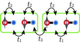
Figure 1: Schematic picture for the spin-Peierls ground state of (TMTTF)₂PF₆ in a 1D chain. 4 dimers, 2 tetramers, and all related transfer integrals are illustrated. Circles and up (down) arrows on them are molecular orbitals of TMTTF and up (down) spins, respectively. A dimer is represented as two circles combined with a flat bar. Neighboring two dimers configure a tetramer which is displayed in the region surrounded by a box. Due to exhibiting charge-orders, a charge rich site and a charge poor site alternate.

We consider a 1D chain of $N_{s}$ sites based on a 1/4-filled hole system with an equal population of spins ($N_{\uparrow}=N_{\downarrow}=N_{s}/4$) at $T=0$. Our Hamiltonian with the PBC (periodic boundary condition) is described as

$$H=-\sum_{j=1}^{N_{s}}\sum_{\sigma}t(j)\left[c_{j+1,\sigma}^{\dagger}c_{j,\sigma}+c_{j,\sigma}^{\dagger}c_{j+1,\sigma}\right]+U\sum_{j=1}^{N_{s}}n_{j,\uparrow}n_{j,\downarrow}+V\sum_{j=1}^{N_{s}}n_{j+1}n_{j},$$ (1)

where $c_{j,\sigma}^{(\dagger)}$ denotes an annihilation (creation) operator of a hole with spin $\sigma=\uparrow,\downarrow$ at the $j$-th site and $n_{j}\equiv n_{j,\uparrow}+n_{j,\downarrow}$ ($n_{j,\sigma}\equiv c_{j,\sigma}^{\dagger}c_{j,\sigma}$). A tetramer formation of (TMTTF)₂PF₆ in the spin-Peierls ground state is classified by utilizing different transfer integrals defined as

$$t(j)=\begin{cases}t_{1}&{\rm for}\;j=4l-2\;\textrm{(inter-dimer), }\\ t_{2}&{\rm for}\;j=4l-1,4l-3\;\textrm{(intra-dimer), }\\ t_{3}&{\rm for}\;j=4l\;\textrm{(inter-tetramer), }\end{cases}$$ (2)

for $1\leq l\leq N_{s}/4$, respectively. The relationship between these transfer integrals and the ground state are schematically illustrated in Fig. 1. According to the Ref. Sawa , $t_{1}/t_{2}=0.862$ and $t_{3}/t_{2}=0.833$ are calculated within the framework of the extended Hückel method Huckel with structural parameters of (TMTTF)₂PF₆ observed by X-ray diffraction experiments at 7 K. In contrast to transfer integrals, to determine Coulomb repulsive interaction strengths $U$ and $V$ is much difficult in general. However, we employ $0.2\leq V/U\leq 0.6$ for $U/t_{2}=5,10$ as typical values of (TMTTF)₂PF₆ Ogata ; Para1 ; Para2 ; Para3 ; Para4 ; Para5 ; Para6 in this article.

Considering a weak photoexcitation where the linear response theory is legitimated, an optical conductivity of given photon energy $\omega>0$ is written as

$$\sigma(\omega)=-\frac{1}{N_{s}\omega}{\rm Im}\left[\langle\psi_{0}|J\frac{1}{\omega+i\eta+E_{0}-H}J|\psi_{0}\rangle\right]\;(\eta\rightarrow 0+),$$ (3)

where $J=i\sum_{j=1}^{N_{s}}\sum_{\sigma}t(j)[c_{j+1,\sigma}^{\dagger}c_{j,\sigma}-c_{j,\sigma}^{\dagger}c_{j+1,\sigma}]$ represents the electrical current operator. Here, $|\psi_{0}\rangle$ is the ground state wavefunction of $H$ in Eq. (1) and $|\psi_{0}\rangle$ is calculated by means of the exact diagonalization method with its energy $E_{0}$.

For the following discussions, we derive free dispersions of $H$ in Eq. (1) ($U=V=0$) for the thermodynamic limit ($N_{s}\rightarrow+\infty$). Using $\alpha,\alpha^{\prime}=\pm$, they have the forms,

$$E_{\alpha,\alpha^{\prime}}(k)=\alpha\sqrt{\frac{t_{1}^{2}+2t_{2}^{2}+t_{3}^{2}}{2}+\alpha^{\prime}\sqrt{\left[\frac{(t_{1}+t_{3})^{2}}{4}+t_{2}^{2}\right](t_{1}-t_{3})^{2}+4t_{1}t_{2}^{2}t_{3}\cos^{2}(2k)}}.$$ (4)

The first Brillouin zone of these dispersions is $-k_{\rm F}\leq k<k_{\rm F}$, where $k_{\rm F}=\pi/4$ denotes a Fermi wave number corresponding to a 1/4-filling.

3 Optical conductivities and electronic excitation energies

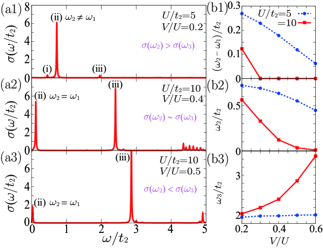
Figure 2: (a1)-(a3) Calculated $\sigma(\omega)$ for $N_{s}=20,\eta/t_{2}=0.01$ under the PBC. Using the well-known order of $t_{2}\sim 0.2$ eV Ogata ; Para4 , our displayed $\omega$ region is $0<\omega\lesssim$ 1 eV which corresponds to a typical $\omega$ range of observations. Three characteristic excitation energies of electrons in the $\omega$ region are illustrated as (i) $\omega_{1}$, (ii) $\omega_{2}$, and (iii) $\omega_{3}$ in the figures. $U,V$ dependences of $\omega_{2}-\omega_{1}$, $\omega_{2}$, and $\omega_{3}$ are shown in (b1), (b2), and (b3), respectively.

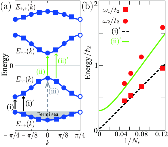
Figure 3: (a) Schematic picture of free dispersions for $N_{s}=16$ on the first Brillouin zone. Solid lines are $E_{\alpha,\alpha^{\prime}}(k)$ in Eq. (4). Filled circles and squares represent allowed discrete wave numbers of the PBC and those of the APBC, respectively, for $N_{s}=16$. Hollowed circles are unavailable discrete wave numbers. (i) is a vertical transition at $k=\pm\pi/4=\pm k_{\rm F}$ and (i)^′ is its nearest transition. All corresponding discrete wave numbers of the transition (i)^′ are $k_{n}^{\rm(i)^{\prime}}=\pm(\pi/4-\pi/N_{s})$ both for $N_{s}=8,16$ under the APBC and $N_{s}=12,20$ under the PBC. (ii) and (iii) are transitions at $k=0$. (ii) also corresponds to the minimum energy gap in the spinless fermion picture. To evaluate the finite size effects of (ii), we choose (ii)^′ as its nearest transition. All corresponding discrete wave numbers of the transition (ii)^′ are $k_{n}^{\rm(ii)^{\prime}}=\pm\pi/N_{s}$ and $k_{n}^{\rm(ii)^{\prime}}$ are, however, only valid for the APBC. (b) Finite size scalings of $\omega_{1},\omega_{2}$ for $N_{s}=8,16$ under the APBC, $N_{s}=12,20$ under the PBC, and $U/t_{2}=5,V/U=0.2$. (i)^′ and (ii)^′ are the same as in (a). The dashed line and the solid line express $\Delta E_{\rm(i)^{\prime}}(N_{s})=E_{-,-}(k_{n}^{\rm(i)^{\prime}})-E_{-,+}(k_{n}^{\rm(i)^{\prime}})$ and $\Delta E_{\rm(ii)^{\prime}}(N_{s})=E_{+,-}(k_{n}^{\rm(ii)^{\prime}})-E_{-,-}(k_{n}^{\rm(ii)^{\prime}})$, respectively, where $E_{\alpha,\alpha^{\prime}}(k)$ are in Eq. (4). For the conventional dimerized model (in Eq. (1) with $t_{3}=t_{1}$), electronic excitation energies of the transitions (i) and (ii) are corresponding to 0 (gapless) and $\Delta_{\rm L}^{\rm di}=2|t_{1}-t_{2}|$, respectively.

Typical results of optical conductivities $\sigma(\omega)$ with $\eta/t_{2}=0.01$ are shown in Figs. 2 (a1)-(a3) and we find that three significant peaks in the low-energy region represented as (i), (ii), and (iii) in the figures characterize $\sigma(\omega)$. Here, we note that our calculations are performed with $N_{s}=20$ for the computational problem although finite size effects remain quintessentially in the order of $1/N_{s}$. Now, we introduce corresponding electronic excitation energies $\omega_{1}$, $\omega_{2}$, and $\omega_{3}$ of the peaks (i), (ii), and (iii), respectively ($\omega_{1}\leq\omega_{2}<\omega_{3}$). Using this, we first investigate $U,V$ dependences of $\sigma(\omega)$ as shown in Figs. 2 (b1)-(b3). As a result, we can classify the structures of $\sigma(\omega)$ into two types. One type is the case of $\omega_{1}\neq\omega_{2}$ and $\sigma(\omega_{2})>\sigma(\omega_{3})$ seen in $U/t_{2}=5$ with $0.2\leq V/U\leq 0.6$ and in $U/t_{2}=10$ with $0.2\leq V/U\lesssim 0.3$. A distinctive $\sigma(\omega)$ of this case is shown in Fig. 1 (a1). Another type is the case of $\omega_{1}=\omega_{2}$ for $U/t_{2}=10$ with $0.3\lesssim V/U\leq 0.6$ and typical results of $\sigma(\omega)$ are shown in Figs. 2 (a2) and (a3). In this case, $\sigma(\omega_{2})>\sigma(\omega_{3})$ for $0.3\lesssim V/U\lesssim 0.4$, $\sigma(\omega_{2})\sim\sigma(\omega_{3})$ for $V/U\sim 0.4$, and otherwise $\sigma(\omega_{2})<\sigma(\omega_{3})$ are satisfied.

From Fig. 2 (b3), $\omega_{3}\rightarrow 2t_{2}$ might be fulfilled for $V\rightarrow 0$ with fixed $U$ or for $U\rightarrow+\infty$ with fixed $V$. Furthermore, $\omega_{3}$ enlarges with increase in $V$. This leads us to judge $\omega_{3}$ as an electronic excitation energy of a COI (charge-ordered insulator) state originates from $U,V$. According to the phase diagram of the conventional dimerized model (in Eq. (1) with $t_{3}=t_{1}$) at $T=0$, the ground state can be divided into a dimer-Mott insulator phase for small $U,V$ and a COI phase for large $U,V$ Ogata ; Para3 . As mentioned in Sect. 1, nature of the spin-Peierls phase of (TMTTF)₂PF₆ partially contains that of the COI phase. In addition to this, the critical point of the metal-COI phase transition is $(U,V)=(+\infty,2t)$ for a 1/4-filled extended Hubbard model (in Eq. (1) with $t_{1}=t_{2}=t_{3}\equiv t$) 14exHubP . Then, the growth of $\omega_{3}$ with respect to finite $V$ for $U\rightarrow+\infty$ can roughly be estimated by $V-2t_{2}$ or, namely, $\omega_{3}\propto V$ and that origin might be related to the COI phase. This feature certainly appears in Fig. 2 (b3), especially, for $U/t_{2}=10$ (in the COI phase).

On the other hand, as seen in Figs. 2 (b1) and (b2), we cannot apply above discussions of $\omega_{3}$ to $U,V$ dependences of $\omega_{1}$ and $\omega_{2}$. However, for the conventional dimerized model (in Eq. (1) with $t_{3}=t_{1}$), peak structures of $\sigma(\omega)$ in the low-energy region have already been manifested within the framework of the exact diagonalization method Mila . According to the Ref. Mila , there are two specific excitation energies of electrons $\omega_{1}^{\rm di}\equiv\Delta_{\rm L}^{\rm di}=2|t_{1}-t_{2}|$ and $\omega_{2}^{\rm di}\equiv\Delta_{\rm F}^{\rm di}=2\sqrt{t_{1}^{2}+t_{2}^{2}}$ ($\omega_{1}^{\rm di}<\omega_{2}^{\rm di}$) which are almost independent in small $U,V$ (not in the COI phase). $\Delta_{\rm L}^{\rm di}$ and $\Delta_{\rm F}^{\rm di}$ are corresponding to vertical transitions of free dispersions at the zone-boundary of the first Brillouin zone and at the Fermi surface in that model, respectively. We note that the transition of $\Delta_{\rm L}^{\rm di}$ is permitted for the spinless fermion picture which is, for instance, valid for $U\rightarrow+\infty$ and $V=0$ OgataShiba . Using this as a reference, we inquire into finite size scalings with $U/t_{2}=5,V/U=0.2$ (not in the COI phase or, in other word, in the regime of weak interactions) which is the minimum parameter set in our calculations and try to grasp the connection between electronic excitation energies ($\omega_{1}$, $\omega_{2}$, $\omega_{3}$) and free dispersions in Eq. (4). For this purpose, all calculations of the finite size scalings are done with the APBC (the anti-periodic boundary condition) for $N_{s}=8$, 16 and the PBC for $N_{s}=12$, 20 due to avoiding forbidden electronic excitations at the zone-boundaries of dispersions in the first Brillouin zone Mila . Here, under the APBC, the first term on the right side of Eq. (1) is just treated as $-\sum_{j=1}^{N_{s}-1}\sum_{\sigma}t(j)[c_{j+1,\sigma}^{\dagger}c_{j,\sigma}+c_{j,\sigma}^{\dagger}c_{j+1,\sigma}]+t(N_{s})[c_{N_{s}+1,\sigma}^{\dagger}c_{N_{s},\sigma}+c_{N_{s},\sigma}^{\dagger}c_{N_{s}+1,\sigma}]$.

Schematic pictures of electronic excitations associated with free dispersions in Eq. (4) and the results of the finite size scalings are shown in Figs. 3 (a) and (b), respectively. Vertical transitions represented as (i), (ii) and (iii) in Fig. 3 (a) are the same as in Fig. 2. Deducing from Fig. 3 (b) and explanations in the caption of Fig. 3, $\omega_{1}$ and $\omega_{2}$ are good agreement with $\Delta E_{\rm(i)^{\prime}}(N_{s})/t_{2}$ and $\Delta E_{\rm(ii)^{\prime}}(N_{s})/t_{2}$, respectively. Then, $\omega_{1}$ in the thermodynamic limit seems to converge on $\Delta_{\rm F}^{\rm tetra}\equiv\Delta E_{\rm(i)^{\prime}}(N_{s}\rightarrow+\infty)=E_{-,-}(\pm k_{\rm F})-E_{-,+}(\pm k_{\rm F})=0.029t_{2}\ll\omega_{1}^{\rm di}=0.276t_{2}$. Here, $\Delta_{\rm F}^{\rm tetra}$ denotes the minimum band gap represented as (i) in Fig. 3 (a) and corresponds to the inter-band transition at the Fermi surface for $N_{s}\rightarrow+\infty$. In a similar fashion, $\omega_{2}$ in the thermodynamic limit seems to converge on $\Delta_{\rm L}^{\rm tetra}\equiv\Delta E_{\rm(ii)^{\prime}}(N_{s}\rightarrow+\infty)=E_{+,-}(0)-E_{-,-}(0)=0.305t_{2}$ expressed as (ii) in Fig. 3 (a) and $\Delta_{\rm L}^{\rm tetra}\sim\omega_{1}^{\rm di}$. This means that, due to $t_{1}\sim t_{3}$, the minimum inter-band gap energy in the spinless fermion picture of our tetrameric model is close to that of the conventional dimerized model (in Eq. (1) with $t_{3}=t_{1}$). Contrary to the above-discussed case of large $U,V$ (strong interactions), $\omega_{3}$ hardly depends on $V$ for $U/t_{2}=5$ as shown in Fig. 2 (b3) and the value $\omega_{3}=1.956t_{2}$ at $U/t_{2}=5$ and $V/U=0.2$ is comparable to $\Delta_{\rm U}^{\rm tetra}\equiv E_{-,-}(0)-E_{-,+}(0)=1.695t_{2}\sim\omega_{2}^{\rm di}=1.320t_{2}$. Here, $\Delta_{\rm U}^{\rm tetra}$ corresponds to the inter-band transition (iii) illustrated in Fig. 3 (a). However, we note that this transition does not physically correspond to the transition of $\omega_{2}^{\rm di}$ for the conventional dimerized model (in Eq. (1) with $t_{3}=t_{1}$).

Consequently, in the thermodynamic limit, our results indicate that optical conductivities with tetramer formation are characterized by three excitation energies of electrons $\omega_{1}\sim\Delta_{\rm F}^{\rm tetra}$, $\omega_{2}\sim\Delta_{\rm L}^{\rm tetra}$, and $\omega_{3}\sim\Delta_{\rm U}^{\rm tetra}$ ($\Delta_{\rm F}^{\rm tetra}<\Delta_{\rm L}^{\rm tetra}<\Delta_{\rm U}^{\rm tetra}$) for not in the COI phase (or weak Coulomb interactions) such as the case of $U/t_{2}=5$ and $V/U\sim 0.2$. On the other hand, for strong Coulomb interactions like $U/t_{2}=10$, $V/U\sim 0.6$ (in the COI phase), $\omega_{1}=\omega_{2}\ll\Delta_{\rm L}^{\rm tetra}$ and $\Delta_{\rm U}^{\rm tetra}\ll\omega_{3}\propto V$ are satisfied. The feature of $\omega_{3}\propto V$ can be regarded as the similar case of the COI phase with the well-known conventional model (in Eq. (1) with $t_{1}=t_{2}=t_{3}\equiv t$). However, the detailed evaluation of $\omega_{1}=\omega_{2}$ ($\ll\Delta_{\rm L}^{\rm tetra}$) in the thermodynamic limit is far difficult due to the strong correlations caused by large $U,V$.

4 Conclusion

In summary, we theoretically calculate the optical conductivity of (TMTTF)₂PF₆ in the spin-Peierls ground state within the framework of the exact diagonalization method at $T=0$. For computations, we treat a $1/4$-filled 1D extended Hubbard model with tetramerization and appropriate parameters which have already been reported. As a result, we clarified that the electronic excitation energies from that spin-Peierls ground state are characterized by $\Delta_{\rm F}^{\rm tetra}$, $\Delta_{\rm L}^{\rm tetra}$, and $\Delta_{\rm U}^{\rm tetra}$ ($\Delta_{\rm F}^{\rm tetra}<\Delta_{\rm L}^{\rm tetra}<\Delta_{\rm U}^{\rm tetra}$) for weak Coulomb interaction strengths (not in the COI phase). From comparison with the results of the conventional dimerized model, the tetramerization newly produces the electronic excitation energy $\Delta_{\rm F}^{\rm tetra}$ which is the lowest gap energy at the Fermi surface on the free dispersions. This can be an instrumental feature which is presented in the optical conductivity to distinguish electronic excitations of dimers from those of tetramers in the low-energy region. However, for strong Coulomb interactions (in the COI phase), apart from the excitation energy which is roughly proportional to $V$, strong correlations drastically affect electronic excitation energies even in the low-energy region and it is hard to evaluate them. Although calculations in this article contain finite size effects to some extent, our results are still useful to understand the effects of tetramerization on the optical properties of (TMTTF)₂PF₆.

- (1) B. Salameh, S. Yasin, M. Dumm, G. Untereiner, L. Montgomery, and M. Dressel, Phys. Rev. B 83, 205126 (2011).
- (2) B. Köhler, E. Rose, M. Dumm, G. Untereiner, and M. Dressel, Phys. Rev. B 84, 035124 (2011).
- (3) K. Medjanik, M. de Souza, D. Kutnyakhov, A. Gloskovskii, J. Müller, M. Lang, J.-P. Pouget, P. F.-Leylekian, A. Moradpour, H.-J. Elmers, and G. Schönhense, Eur. Phys. J. B 87, 256 (2014).
- (4) S. Tomić and M. Dressel, Rep. Prog. Phys. 78, 096501 (2015).
- (5) I. Voloshenko, M. Herter, R. Beyer, A. Pustogow, and M. Dressel, J. Phys.: Condens. Matter 29, 115601 (2017).
- (6) H. Wilhelm, D. Jaccard, R. Duprat, C. Bourbonnais, D. Jérome, J. Moser, C. Carcel, and J. M. Fabre, Eur. Phys. J. B 21, 175 (2001).
- (7) L. Degiorgi and D. Jérome, J. Phys. Soc. Jpn. 75, 051004 (2006).
- (8) H. Seo, J. Merino, H. Yoshioka, and M. Ogata, J. Phys. Soc. Jpn. 75, 051009 (2006).
- (9) F. Iwase, K. Sugiura, K. Furukawa, and T. Nakamura, J. Phys. Soc. Jpn. 78, 104717 (2009).
- (10) A. Pustogow, T. Peterseim, S. Kolatschek, L. Engel, and M. Dressel, Phys. Rev. B 94, 195125 (2016).
- (11) S. Kitou, T. Fujii, T. Kawamoto, N. Katayama, S. Maki, E. Nishibori, K. Sugimoto, M. Takata, T. Nakamura, and H. Sawa, Phys. Rev. Lett. 119, 065701 (2017).
- (12) V. Vescoli, L. Degiorgi, W. Henderson, G. Grüner, K. P. Starkey, and L. K. Montgomery, Science 281, 1181 (1998); V. Vescoli, L. Degiorgi, K. P. Starkey, and L. K. Montgomery, Solid State Communications 111, 507 (1999).
- (13) A. Pashkin, M. Dressel, M. Hanfland, and C. A. Kuntscher, Phys. Rev. B 81, 125109 (2010).
- (14) Y. Naitoh, Y. Kawakami, T. Ishikawa, Y. Sagae, H. Itoh, K. Yamamoto, T. Sasaki, M. Dressel, S. Ishihara, Y. Tanaka, K. Yonemitsu, and S. Iwai, Phys. Rev. B 93, 165126 (2016).
- (15) T. Mori, A Kobayashi, Y Sasaki, H. Kobayashi, G. Saito, and H. Inokuchi, Bull. Chem. Soc. Jpn. 57, 627 (1984).
- (16) L. Ducasse, M. Abderrabbat, J. Hoaraut, M. Pesquert, B. Gallois, and J. Gaultier, J. Phys. C: Solid State Phys. 19, 3805 (1986).
- (17) F. Mila, Phys. Rev. B 52, 4788 (1995).
- (18) M. Tsuchiizu, H. Yoshioka, and Y. Suzumura, J. Phys. Soc. Jpn. 68, 1809 (1999); J. Phys. Soc. Jpn. 70, 1460 (2001).
- (19) S. Nishimoto, M. Takahashi, and Y. Ohta, J. Phys. Soc. Jpn. 69, 1594 (2000).
- (20) K. Furukawa, K. Sugiura, F. Iwase, and T. Nakamura, Phys. Rev. B 83, 184419 (2011).
- (21) G. Giovannetti, S. Kumar, J.-P. Pouget, and M. Capone, Phys. Rev. B 85, 205146 (2012).
- (22) F. Mila and X. Zotos, Eur. Phys. Lett. 24, 133 (1993).
- (23) J. Favand and F. Mila, Phys. Rev. B 54, 10425 (1996).
- (24) M. Ogata and H. Shiba, Phys. Rev. B 43, 8401 (1991).