Quasi-Monte Carlo Variational Inference

Abstract

Many machine learning problems involve Monte Carlo gradient estimators. As a prominent example, we focus on Monte Carlo variational inference (mcvi) in this paper. The performance of mcvi crucially depends on the variance of its stochastic gradients. We propose variance reduction by means of Quasi-Monte Carlo (qmc) sampling. qmc replaces $N$ i.i.d. samples from a uniform probability distribution by a deterministic sequence of samples of length $N$. This sequence covers the underlying random variable space more evenly than i.i.d. draws, reducing the variance of the gradient estimator. With our novel approach, both the score function and the reparameterization gradient estimators lead to much faster convergence. We also propose a new algorithm for Monte Carlo objectives, where we operate with a constant learning rate and increase the number of qmc samples per iteration. We prove that this way, our algorithm can converge asymptotically at a faster rate than sgd. We furthermore provide theoretical guarantees on qmc for Monte Carlo objectives that go beyond mcvi, and support our findings by several experiments on large-scale data sets from various domains.

1 Introduction

In many situations in machine learning and statistics, we encounter objective functions which are expectations over continuous distributions. Among other examples, this situation occurs in reinforcement learning (Sutton and Barto, 1998) and variational inference (Jordan et al., 1999). If the expectation cannot be computed in closed form, an approximation can often be obtained via Monte Carlo (mc) sampling from the underlying distribution. As most optimization procedures rely on the gradient of the objective, a mc gradient estimator has to be built by sampling from this distribution. The finite number of mc samples per gradient step introduces noise. When averaging over multiple samples, the error in approximating the gradient can be decreased, and thus its variance reduced. This guarantees stability and fast convergence of stochastic gradient descent (sgd).

Certain objective functions require a large number of mc samples per stochastic gradient step. As a consequence, the algorithm gets slow. It is therefore desirable to obtain the same degree of variance reduction with fewer samples. This paper proposes the idea of using Quasi-Monte Carlo (qmc) samples instead of i.i.d. samples to achieve this goal.

A qmc sequence is a deterministic sequence which covers a hypercube $[0,1]^{d}$ more regularly than random samples. When using a qmc sequence for Monte Carlo integration, the mean squared error (MSE) decreases asymptotically with the number of samples $N$ as ${\cal O}(N^{-2}(\log N)^{2d-2})$ (Leobacher and Pillichshammer, 2014). In contrast, the naive mc integration error decreases as ${\cal O}(N^{-1})$. Since the cost of generating $N$ qmc samples is ${\cal O}(N\log N$), this implies that a much smaller number of operations per gradient step is required in order to achieve the same precision (provided that $N$ is large enough). Alternatively, we can achieve a larger variance reduction with the same number of samples, allowing for larger gradient steps and therefore also faster convergence. This paper investigates the benefits of this approach both experimentally and theoretically.

Our ideas apply in the context of Monte Carlo variational inference (mcvi), a set of methods which make approximate Bayesian inference scalable and easy to use. Variance reduction is an active area of research in this field. Our algorithm has the advantage of being very general; it can be easily implemented in existing software packages such as STAN and Edward (Carpenter et al., 2017; Tran et al., 2016). In Appendix D we show how our approach can be easily implemented in your existing code.

The main contributions are as follows:

• We investigate the idea of using qmc sequences for Monte Carlo variational inference. While the usage of qmc for vi has been suggested in the outlook section of Ranganath et al. (2014), to our knowledge, we are the first to actually investigate this approach both theoretically and experimentally.

• We show that when using a randomized version of qmc (rqmc), the resulting stochastic gradient is unbiased and its variance is asymptotically reduced. We also show that when operating sgd with a constant learning rate, the stationary variance of the iterates is reduced by a factor of $N$, allowing us to get closer to the optimum.

• We propose an algorithm which operates at a constant learning rate, but increases the number of rqmc samples over iterations. We prove that this algorithm has a better asymptotic convergence rate than sgd.

• Based on three different experiments and for two popular types of gradient estimators we illustrate that our method allows us to train complex models several orders of magnitude faster than with standard mcvi.

Our paper is structured as follows. Section 2 reviews related work. Section 3 explains our method and exhibits our theoretical results. In Section 4 we describe our experiments and show comparisons to other existing approaches. Finally, Section 5 concludes and lays out future research directions.

2 Related Work

Monte Carlo Variational Inference (MCVI)

Since the introduction of the score function (or REINFORCE) gradient estimator for variational inference (Paisley et al., 2012; Ranganath et al., 2014), Monte Carlo variational inference has received an ever-growing attention, see Zhang et al. (2017a) for a recent review. The introduction of the gradient estimator made vi applicable to non-conjugate models but highly depends on the variance of the gradient estimator. Therefore various variance reduction techniques have been introduced; for example Rao-Blackwellization and control variates, see Ranganath et al. (2014) and importance sampling, see Ruiz et al. (2016a); Burda et al. (2016).

At the same time the work of Kingma and Welling (2014); Rezende et al. (2014) introduced reparameterization gradients for mcvi, which typically exhibits lower variance but are restricted to models where the variational family can be reparametrized via a differentiable mapping. In this sense mcvi based on score function gradient estimators is more general but training the algorithm is more difficult. A unifying view is provided by Ruiz et al. (2016b). Miller et al. (2017) introduce a modification of the reparametrized version, but relies itself on assumptions on the underlying variational family. Roeder et al. (2017) propose a lower variance gradient estimator by omitting a term of the elbo. The idea of using qmc in order to reduce the variance has been suggested by Ranganath et al. (2014) and Ruiz et al. (2016a) and used for a specific model by Tran et al. (2017), but without a focus on analyzing or benchmarking the method.

Quasi-Monte Carlo and Stochastic Optimization

Besides the generation of random samples for approximating posterior distributions (Robert and Casella, 2013), Monte Carlo methods are used for calculating expectations of intractable integrals via the law of large numbers. The error of the integration with random samples goes to zero at a rate of $\mathcal{O}(N^{-1})$ in terms of the MSE. For practical application this rate can be too slow. Faster rates of convergence in reasonable dimensions can be obtained by replacing the randomness by a deterministic sequence, also called Quasi-Monte Carlo.

Compared to Monte Carlo and for sufficiently regular functions, qmc reaches a faster rate of convergence of the approximation error of an integral. Niederreiter (1992); L’Ecuyer and Lemieux (2005); Leobacher and Pillichshammer (2014); Dick et al. (2013) provide excellent reviews on this topic. From a theoretical point of view, the benefits of qmc vanish in very high dimensions. Nevertheless, the error bounds are often too pessimistic and in practice, gains are observed up to dimension $150$, see Glasserman (2013).

qmc has frequently been used in financial applications (Glasserman, 2013; Joy et al., 1996; Lemieux and L’Ecuyer, 2001). In statistics, some applications include particle filtering (Gerber and Chopin, 2015), approximate Bayesian computation (Buchholz and Chopin, 2017), control functionals (Oates and Girolami, 2016) and Bayesian optimal design (Drovandi and Tran, 2018). Yang et al. (2014) used qmc in the context of large scale kernel methods.

Stochastic optimization has been pioneered by the work of Robbins and Monro (1951). As stochastic gradient descent suffers from noisy gradients, various approaches for reducing the variance and adapting the step size have been introduced (Johnson and Zhang, 2013; Kingma and Ba, 2015; Defazio et al., 2014; Duchi et al., 2011; Zhang et al., 2017b). Extensive theoretical results on the convergence of stochastic gradients algorithms are provided by Moulines and Bach (2011). Mandt et al. (2017) interpreted stochastic gradient descent with constant learning rates as approximate Bayesian inference. Some recent reviews are for example Bottou et al. (2016); Nesterov (2013). Naturally, concepts from qmc can be beneficial to stochastic optimization. Contributions on exploiting this idea are e.g. Gerber and Bornn (2017) and Drew and Homem-de Mello (2006).

3 Quasi-Monte Carlo Variational Inference

In this Section, we introduce Quasi-Monte Carlo Variational Inference (qmcvi), using randomized qmc (rqmc) for variational inference. We review mcvi in Section 3.1. rqmc and the details of our algorithm are exposed in Section 3.2. Theoretical results are given in Section 3.3.

3.1 Background: Monte Carlo Variational Inference

Variational inference (vi) is key to modern probabilistic modeling and Bayesian deep learning (Jordan et al., 1999; Blei et al., 2017; Zhang et al., 2017a). In Bayesian inference, the object of interest is a posterior distribution of latent variables $\mathbf{z}$ given observations $\mathbf{x}$. vi approximates Bayesian inference by an optimization problem which we can solve by (stochastic) gradient ascent (Jordan et al., 1999; Hoffman et al., 2013).

In more detail, vi builds a tractable approximation of the posterior $p(\mathbf{z}|\mathbf{x})$ by minimizing the $\mathrm{KL}$-divergence between a variational family $q(\mathbf{z}|\mathbf{\lambda})$, parametrized by free parameters $\mathbf{\lambda}\in\mathbb{R}^{d}$, and $p(\mathbf{z}|\mathbf{x})$. This is equivalent to maximizing the so-called evidence lower bound (elbo):

$$\mathcal{L}(\mathbf{\lambda})=\mathbb{E}_{q(\mathbf{z}|\mathbf{\lambda})}[\log p(\mathbf{x},\mathbf{z})-\log q(\mathbf{z}|\mathbf{\lambda})].$$ (1)

In classical variational inference, the expectations involved in (1) are carried out analytically (Jordan et al., 1999). However, this is only possible for the fairly restricted class of so-called conditionally conjugate exponential family models (Hoffman et al., 2013). More recently, black-box variational methods have gained momentum, which make the analytical evaluation of these expectation redundant, and which shall be considered in this paper.

Maximizing the objective (1) is often based on a gradient ascent scheme. However, a direct differentiation of the objective (1) with respect to $\mathbf{\lambda}$ is not possible, as the measure of the expectation depends on this parameter. The two major approaches for overcoming this issue are the score function estimator and the reparameterization estimator.

Score Function Gradient

The score function gradient (also called REINFORCE gradient) (Ranganath et al., 2014) expresses the gradient as expectation with respect to $q(\mathbf{z}|\mathbf{\lambda})$ and is given by

$$\nabla_{\mathbf{\lambda}}\mathcal{L}(\mathbf{\lambda})\\ =\mathbb{E}_{q(\mathbf{z}|\mathbf{\lambda})}[\nabla_{\mathbf{\lambda}}\log q(\mathbf{z}|\mathbf{\lambda})\left(\log p(\mathbf{x},\mathbf{z})-\log q(\mathbf{z}|\mathbf{\lambda})\right)].$$ (2)

The gradient estimator is obtained by approximating the expectation with independent samples from the variational distribution $q(\mathbf{z}|\mathbf{\lambda})$. This estimator applies to continuous and discrete variational distributions.

Reparameterization Gradient

The second approach is based on the reparametrization trick (Kingma and Welling, 2014), where the distribution over $\mathbf{z}$ is expressed as a deterministic transformation of another distribution over a noise variable $\mathbf{\varepsilon}$, hence $\mathbf{z}=g_{\mathbf{\lambda}}(\varepsilon)$ where $\mathbf{\varepsilon}\sim p(\mathbf{\varepsilon})$. Using the reparameterization trick, the elbo is expressed as expectation with respect to $p(\varepsilon)$ and the derivative is moved inside the expectation:

$$\nabla_{\mathbf{\lambda}}\mathcal{L}(\mathbf{\lambda})\\ =\mathbb{E}_{p(\mathbf{\varepsilon})}[\nabla_{\mathbf{\lambda}}\log p(\mathbf{x},g_{\mathbf{\lambda}}(\mathbf{\varepsilon}))-\nabla_{\mathbf{\lambda}}\log q(g_{\mathbf{\lambda}}(\mathbf{\varepsilon})|\mathbf{\lambda})].$$ (3)

The expectation is approximated using a mc sum of independent samples from $p(\varepsilon$). In its basic form, the estimator is restricted to distributions over continuous variables.

MCVI

In the general setup of mcvi considered here, the gradient of the elbo is represented as an expectation $\nabla_{\mathbf{\lambda}}\mathcal{L}(\mathbf{\lambda})\\ =\mathbb{E}[g_{\tilde{\mathbf{z}}}(\lambda)]$ over a random variable $\tilde{\mathbf{z}}$. For the score function estimator we choose $g$ according to Equation (2) with $\tilde{\mathbf{z}}=\mathbf{z}$ and for the reparameterization gradient according to Equation (3) with $\tilde{\mathbf{z}}=\mathbf{\varepsilon}$, respectively. This allows us to obtain a stochastic estimator of the gradient by an average over a finite sample $\{\tilde{\mathbf{z}}_{1},\cdots,\tilde{\mathbf{z}}_{N}\}$ as $\hat{g}_{N}(\mathbf{\lambda}_{t})=(1/N)\sum_{i=1}^{N}g_{\tilde{\mathbf{z}}_{i}}(\mathbf{\lambda}_{t})$.This way, the elbo can be optimized by stochastic optimization. This is achieved by iterating the sgd updates with decreasing step sizes $\alpha_{t}$:

$$\mathbf{\lambda}_{t+1}=\mathbf{\lambda}_{t}+\alpha_{t}\hat{g}_{N}(\mathbf{\lambda}_{t}).$$ (4)

The convergence of the gradient ascent scheme in (4) tends to be slow when gradient estimators have a high variance. Therefore, various approaches for reducing the variance of both gradient estimators exist; e.g. control variates (cv), Rao-Blackwellization and importance sampling. However these variance reduction techniques do not improve the $\mathcal{O}(N^{-1})$ rate of the MSE of the estimator, except under some restrictive conditions (Oates et al., 2017). Moreover, the variance reduction schemes must often be tailored to the problem at hand.

3.2 Quasi-Monte Carlo Variational Inference

Quasi Monte Carlo

Low discrepancy sequences, also called qmc sequences, are used for integrating a function $\psi$ over the $[0,1]^{d}$ hypercube. When using standard i.i.d. samples on $[0,1]^{d}$, the error of the approximation is $\mathcal{O}(N^{-1})$. qmc achieves a rate of convergence in terms of the MSE of $\mathcal{O}\left(N^{-2}(\log N)^{2d-2}\right)$ if $\psi$ is sufficiently regular (Leobacher and Pillichshammer, 2014). This is achieved by a deterministic sequence that covers $[0,1]^{d}$ more evenly.

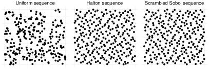
On a high level, qmc sequences are constructed such that the number of points that fall in a rectangular volume is proportional to the volume. This idea is closely linked to stratification. Halton sequences e.g. are constructed using coprime numbers (Halton, 1964). Sobol sequences are based on the reflected binary code (Antonov and Saleev, 1979). The exact construction of qmc sequences is quite involved and we refer to Niederreiter (1992); Leobacher and Pillichshammer (2014); Dick et al. (2013) for more details.

The approximation error of qmc increases with the dimension, and it is difficult to quantify. Carefully reintroducing randomness while preserving the structure of the sequence leads to randomized qmc. rqmc sequences are unbiased and the error can be assessed by repeated simulation. Moreover, under slightly stronger regularity conditions on $F$ we can achieve rates of convergence of $\mathcal{O}(N^{-2})$ (Gerber, 2015). For illustration purposes, we show different sequences in Figure 1. In Appendix A we provide more technical details.

qmc or rqmc can be used for integration with respect to arbitrary distributions by transforming the initial sequence on $[0,1]^{d}$ via a transformation $\Gamma$ to the distribution of interest. Constructing the sequence typically costs $\mathcal{O}(N\log N)$ (Gerber and Chopin, 2015).

Figure 1: mc (left), qmc (center) and rqmc (right) sequences of length $N=256$ on $[0,1]^{2}$. qmc and rqmc tend to cover the target space more evenly.

QMC and VI

We suggest to replace $N$ independent mc samples for computing $\hat{g}_{N}(\mathbf{\lambda}_{t})$ by an rqmc sequence of the same length. With our approach, the variance of the gradient estimators becomes $\mathcal{O}(N^{-2})$, and the costs for creating the sequence is $\mathcal{O}(N\log N)$. The incorporation of rqmc in vi is straightforward: instead of sampling $\tilde{\mathbf{z}}$ as independent mc samples, we generate a uniform rqmc sequence $\mathbf{u}_{1},\cdots,\mathbf{u}_{N}$ and transform this sequence via a mapping $\Gamma$ to the original random variable $\tilde{\mathbf{z}}=\Gamma(\mathbf{u})$. Using this transformation we obtain the rqmc gradient estimator

$$\hat{g}_{N}(\mathbf{\lambda}_{t})=(1/N)\sum_{i=1}^{N}g_{\Gamma(\mathbf{u}_{i})}(\mathbf{\lambda}).$$ (5)

From a theoretical perspective, the function $\mathbf{u}\mapsto g_{\Gamma(\mathbf{u})}(\mathbf{\lambda})$ has to be sufficiently smooth for all $\mathbf{\lambda}$. For commonly used variational families this transformation is readily available. Although evaluating these transforms adds computational overhead, we found this cost negligible in practice. For example, in order to sample from a multivariate Gaussian $\mathbf{z}_{n}\sim\mathcal{N}(\mathbf{\mu},\Sigma)$, we generate an rqmc squence $\mathbf{u}_{n}$ and apply the transformation $\mathbf{z}_{n}=\Phi^{-1}(\mathbf{u}_{n})\Sigma^{1/2}+\mathbf{\mu}$, where $\Sigma^{1/2}$ is the Cholesky decomposition of $\Sigma$ and $\Phi^{-1}$ is the component-wise inverse cdf of a standard normal distribution. Similar procedures are easily obtained for exponential, Gamma, and other distributions that belong to the exponential family. Algorithm 1 summarizes the procedure.

1

Input: Data $\mathbf{x}$, model $p(\mathbf{x},\mathbf{z})$, variational family $q(\mathbf{z}|\lambda)$

Result: Variational parameters $\mathbf{\lambda}^{*}$

2 while not converged do

3       Generate uniform rqmc sequence $\mathbf{u}_{1:N}$

4       Transform the sequence via $\Gamma$

5       Estimate the gradient $\hat{g}_{N}(\mathbf{\lambda}_{t})=\frac{1}{N}\sum_{i=1}^{N}g_{\Gamma(\mathbf{u}_{i})}(\mathbf{\lambda}_{t})$

6       Update $\mathbf{\lambda}_{t+1}=\mathbf{\lambda}_{t}+\alpha_{t}$ $\hat{g}_{N}(\mathbf{\lambda}_{t})$

Algorithm 1 Quasi-Monte Carlo Variational Inference

rqmc samples can be generated via standard packages such as randtoolbox (Christophe and Petr, 2015), available in R. Existing mcvi algorithms are adapted by replacing the random variable sampler by an rqmc version. Our approach reduces the variance in mcvi and applies in particular to the reparametrization gradient estimator and the score function estimator. rqmc can in principle be combined with additional variance reduction techniques such as cv, but care must be taken as the optimal cv for rqmc are not the same as for mc (Hickernell et al., 2005).

3.3 Theoretical Properties of QMCVI

In what follows we give a theoretical analysis of using rqmc in stochastic optimization. Our results apply in particular to vi but are more general.

qmcvi leads to faster convergence in combination with Adam (Kingma and Ba, 2015) or Adagrad (Duchi et al., 2011), as we will show empirically in Section 4. Our analysis, presented in this section, underlines this statement for the simple case of sgd with fixed step size in the Lipschitz continuous (Theorem 1) and strongly convex case (Theorem 2). We show that for $N$ sufficiently large, sgd with rqmc samples reaches regions closer to the true optimizer of the elbo. Moreover, we obtain a faster convergence rate than sgd when using a fixed step size and increasing the sample size over iterations (Theorem 3).

RQMC for Optimizing Monte Carlo Objectives

We step back from black box variational inference and consider the more general setup of optimizing Monte Carlo objectives. Our goal is to minimize a function $F(\lambda)$, where the optimizer has only access to a noisy, unbiased version $\hat{F}_{N}(\mathbf{\lambda})$, with $\mathbb{E}[\hat{F}_{N}(\mathbf{\lambda})]=F(\mathbf{\lambda})$ and access to an unbiased noisy estimator of the gradients $\hat{g}_{N}(\mathbf{\lambda})$, with $\mathbb{E}[\hat{g}_{N}(\mathbf{\lambda})]=\nabla F(\mathbf{\lambda})$. The optimum of $F(\lambda)$ is $\mathbf{\lambda}^{\star}$.

We furthermore assume that the gradient estimator $\hat{g}_{N}(\mathbf{\lambda})$ has the form as in Eq. 5, where $\Gamma$ is a reparameterization function that converts uniform samples from the hypercube into samples from the target distribution. In this paper, $\mathbf{u}_{1},\cdots,\mathbf{u}_{N}$ is an rqmc sequence.

In the following theoretical analysis, we focus on sgd with a constant learning rate $\alpha$. The optimal value $\mathbf{\lambda}^{\star}$ is approximated by sgd using the update rule

$$\mathbf{\lambda}_{t+1}=\mathbf{\lambda}_{t}-\alpha\hat{g}_{N}(\mathbf{\lambda}_{t}).$$ (6)

Starting from $\mathbf{\lambda}_{1}$ the procedure is iterated until $|\hat{F}_{N}(\mathbf{\lambda}_{t})-\hat{F}_{N}(\mathbf{\lambda}_{t+1})|\leq\epsilon$, for a small threshold $\epsilon$. The quality of the approximation $\mathbf{\lambda}_{T}\approx\mathbf{\lambda}^{\star}$ crucially depends on the variance of the estimator $\hat{g}_{N}$ (Johnson and Zhang, 2013).

Intuitively, the variance of $\hat{g}_{N}(\mathbf{\lambda})$ based on an rqmc sequence will be $\mathcal{O}(N^{-2})$ and thus for $N$ large enough, the variance will be smaller than for the mc counterpart, that is $\mathcal{O}(N^{-1})$. This will be beneficial to the optimization procedure defined in (6). Our following theoretical results are based on standard proof techniques for stochastic approximation, see e.g. Bottou et al. (2016).

Stochastic Gradient Descent with Fixed Step Size

In the case of functions with Lipschitz continuous derivatives, we obtain the following upper bound on the norm of the gradients.

Theorem 1

Let $F$ be a function with Lipschitz continuous derivatives, i.e. there exists $L>0$ s.t. $\forall\mathbf{\lambda},\overline{\mathbf{\lambda}}$ $\|\nabla F(\mathbf{\lambda})-\nabla F(\overline{\mathbf{\lambda}})\|^{2}_{2}\leq L\|\mathbf{\lambda}-\overline{\mathbf{\lambda}}\|^{2}_{2}$, let $U_{N}=\{\mathbf{u}_{1},\cdots,\mathbf{u}_{N}\}$ be an rqmc sequence and let $\forall\mathbf{\lambda}$, $G:\mathbf{u}\mapsto g_{\Gamma(\mathbf{u})}(\mathbf{\lambda})$ has cross partial derivatives of up to order $d$. Let the constant learning rate $\alpha<2/L$ and let $\mu=1-\alpha L/2$. Then $\forall\mathbf{\lambda},\operatorname{tr}\operatorname{Var}_{U_{N}}[\hat{g}_{N}(\mathbf{\lambda})]\leq M_{V}\times r(N)$, where $M_{V}<\infty$ and $r(N)=\mathcal{O}\left(N^{-2}\right)$ and

$$\frac{\sum_{t=1}^{T}\mathbb{E}\|\nabla F(\mathbf{\lambda}_{t})\|^{2}_{2}}{T}\\ \leq\frac{1}{2\mu}\alpha LM_{V}r(N)+\frac{F(\mathbf{\lambda}_{1})-F(\mathbf{\lambda}^{\star})}{\alpha\mu T},$$

where $\mathbf{\lambda}_{t}$ is iteratively defined in (6). Consequently,

$$\lim_{T\rightarrow\infty}\frac{\sum_{t=1}^{T}\mathbb{E}\|\nabla F(\mathbf{\lambda}_{t})\|^{2}_{2}}{T}\leq\frac{1}{2\mu}\alpha LM_{V}r(N).$$ (7)

Equation (7) underlines the dependence of the sum of the norm of the gradients on the variance of the gradients. The better the gradients are estimated, the closer one gets to the optimum where the gradient vanishes. As the dependence on the sample size becomes $\mathcal{O}\left(N^{-2}\right)$ for an rqmc sequence instead of $1/N$ for a mc sequence, the gradient is more precisely estimated for $N$ large enough.

We now study the impact of a reduced variance on sgd with a fixed step size and strongly convex functions. We obtain an improved upper bound on the optimality gap.

Theorem 2

Let $F$ have Lipschitz continuous derivatives and be a strongly convex function, i.e. there exists a constant $c>0$ s.t. $\forall\mathbf{\lambda},\overline{\mathbf{\lambda}}$ $F(\overline{\mathbf{\lambda}})\geq F(\mathbf{\lambda})+\nabla F(\mathbf{\lambda})^{T}(\mathbf{\lambda}-\overline{\mathbf{\lambda}})+\frac{1}{2}c\|\mathbf{\lambda}-\overline{\mathbf{\lambda}}\|^{2}_{2}$, let $U_{N}=\{\mathbf{u}_{1},\cdots,\mathbf{u}_{N}\}$ be an rqmc sequence and let $\forall\mathbf{\lambda},G:\mathbf{u}\mapsto g_{\Gamma(\mathbf{u})}(\mathbf{\lambda})$ be as in Theorem 1. Let the constant learning rate $\alpha<\frac{1}{2c}$ and $\alpha<\frac{2}{L}$. Then the expected optimality gap satisfies, $\forall t\geq 0$,

$$\mathbb{E}[F(\mathbf{\lambda}_{t+1})-F(\mathbf{\lambda}^{\star})]\\ \leq\left[\left(\frac{\alpha^{2}L}{2}-\alpha\right)2c+1\right]\times\mathbb{E}[F_{N}(\mathbf{\lambda}_{t})-F(\mathbf{\lambda}^{\star})]\\ +\frac{1}{2}L\alpha^{2}\left[M_{V}r(N)\right].$$

Consequently,

$$\lim_{T\rightarrow\infty}\mathbb{E}[F(\mathbf{\lambda}_{T})-F(\mathbf{\lambda}^{\star})]\leq\frac{\alpha L}{4c-\alpha Lc}\left[M_{V}r(N)\right].$$

The previous result has the following interpretation. The expected optimality gap between the last iteration $\mathbf{\lambda}_{T}$ and the true minimizer $\mathbf{\lambda}^{\star}$ is upper bounded by the magnitude of the variance. The smaller this variance, the closer we get to $\mathbf{\lambda}^{\star}$. Using rqmc we gain a factor $1/N$ in the bound.

Increasing Sample Size Over Iterations

While sgd with a fixed step size and a fixed number of samples per gradient step does not converge, convergence can be achieved when increasing the number of samples used for estimating the gradient over iterations. As an extension of Theorem 2, we show that a linear convergence is obtained while increasing the sample size at a slower rate than for mc sampling.

Theorem 3

Assume the conditions of Theorem 2 with the modification $\alpha\leq\min\{1/c,1/L\}$. Let $1-\alpha c/2<\xi^{2}=\frac{1}{\tau^{2}}<1$. Use an increasing sample size $N_{t}=\underline{N}+\lceil\tau^{t}\rceil$, where $\underline{N}<\infty$ is defined in Appendix B.3. Then $\forall t\in\mathbb{N},\exists\hat{M}_{V}<\infty,$

$$\operatorname{tr}\operatorname{Var}_{U_{N}}[\hat{g}_{N_{t}}(\mathbf{\lambda})]\leq\hat{M}_{V}\times\frac{1}{\tau^{2t}}$$

and

$$\mathbb{E}[F(\mathbf{\lambda}_{t+1})-F(\mathbf{\lambda}^{\star})]\leq\omega\xi^{2t},$$

where $\omega=\max\{\alpha L\hat{M}_{V}/c,F(\mathbf{\lambda}_{1})-F(\mathbf{\lambda}^{\star})\}$.

This result compares favorably with a standard result on the linear convergence of sgd with fixed step size and strongly convex functions (Bottou et al., 2016). For mc sampling one obtains a different constant $\tilde{\omega}$ and an upper bound with $\xi^{t}$ and not $\xi^{2t}$. Thus, besides the constant factor, rqmc samples allow us to close the optimality gap faster for the same geometric increase in the sample size $\tau^{t}$ or to use $\tau^{t/2}$ to obtain the same linear rate of convergence as mc based estimators.

Other Remarks

The reduced variance in the estimation of the gradients should allow us to make larger moves in the parameter space. This is for example achieved by using adaptive step size algorithms as Adam (Kingma and Ba, 2015), or Adagrad (Duchi et al., 2011). However, the theoretical analysis of these algorithms is beyond the scope of this paper.

Also, note that it is possible to relax the smoothness assumptions on $G$ while supposing only square integrability. Then one obtains rates in $o(N^{-1})$. Thus, rqmc yields always a faster rate than mc, regardless of the smoothness. See Appendix A for more details.

In the previous analysis, we have assumed that the entire randomness in the gradient estimator comes from the sampling of the variational distribution. In practice, additional randomness is introduced in the gradient via mini batch sampling. This leads to a dominating term in the variance of $\mathcal{O}(K^{-1})$ for mini batches of size $K$. Still, the part of the variance related to the variational family itself is reduced and so is the variance of the gradient estimator as a whole.

4 Experiments

We study the effectiveness of our method in three different settings: a hierarchical linear regression, a multi-level Poisson generalized linear model (GLM) and a Bayesian neural network (BNN). Finally, we confirm the result of Theorem 3, which proposes to increase the sample size over iterations in qmcvi for faster asymptotic convergence.

Figure 2: Toy: experiment 4.1. elbo optimization path using Adam and variance of the stochastic gradient using the rqmc based gradient estimator using 10 samples (ours, in red) and the mc based estimator using 10 samples (blue) and 100 samples (black), respectively. The upper panel corresponds to the reparameterization gradient and the lower panel to the score function gradient estimator. For both versions of mcvi, using rqmc samples (proposed) leads to variance reduction and faster convergence.

Figure 3: Frisk: experiment 4.2. Left, the optimization path of the elbo is shown using Adam with the rqmc, mc and cv based reparameterization gradient estimator, respectively. Right, the gradient variances as function of time are reported. In the case of using 10 samples (dashed lines) rqmc (ours) outperforms the baselines in terms of speed while the cv based method exhibits lowest gradient variance. When increasing the sample size to 50 (solid lines) for all methods, rqmc converges closer to the optimum than the baselines while having lowest gradient variance.

Figure 4: BNN: experiment 4.3. Left, the optimization path of the elbo is shown using Adam with the rqmc, mc and cv based reparameterization gradient estimator, respectively. Right, the gradient variances as function of time are reported. rqmc (ours) based on 10 samples outperforms the baselines in terms of speed. rqmc with 50 samples is bit slower but converges closer to the optimum as its gradient variance is up to 3 orders of magnitude lower than for the baselines.

Setup

In the first three experiments we optimize the elbo using the Adam optimizer (Kingma and Ba, 2015) with the initial step size set to $0.1$, unless otherwise stated. The rqmc sequences are generated through a python interface to the R package randtoolbox (Christophe and Petr, 2015). In particular we use scrambled Sobol sequences. The gradients are calculated using an automatic differentiation toolbox. The elbo values are computed by using $10,000$ mc samples, the variance of the gradient estimators is estimated by resampling the gradient $1000$ times in each optimization step and computing the empirical variance.

Benchmarks

The first benchmark is the vanilla mcvi algorithm based on ordinary mc sampling. Our method qmcvi replaces the mc samples by rqmc sequences and comes at almost no computational overhead (Section 3).

Our second benchmark in the second and third experiment is the control variate (cv) approach of Miller et al. (2017), where we use the code provided with the publication. In the first experiment, this comparison is omitted since the method of Miller et al. (2017) does not apply in this setting due to the non-Gaussian variational distribution.

Main Results

We find that our approach generally leads to a faster convergence compared to our baselines due to a decreased gradient variance. For the multi-level Poisson GLM experiment, we also find that our rqmc algorithm converges to a better local optimum of the elbo. As proposed in Theorem 3, we find that increasing the sample size over iteration in qmcvi leads to a better asymptotic convergence rate than in mcvi.

4.1 Hierarchical Linear Regression

We begin the experiments with a toy model of hierarchical linear regression with simulated data. The sampling process for the outputs $y_{i}$ is $y_{i}\leavevmode\nobreak\ \sim\leavevmode\nobreak\ \mathcal{N}(\mathbf{x}_{i}^{\top}\mathbf{b}_{i},\epsilon),\;\mathbf{b}_{i}\leavevmode\nobreak\ \sim\leavevmode\nobreak\ \mathcal{N}(\mathbf{\mu}_{\beta},\sigma_{\beta}).$ We place lognormal hyper priors on the variance of the intercepts $\sigma_{\beta}$ and on the noise $\epsilon$; and a Gaussian hyper prior on $\mathbf{\mu}_{\beta}$. Details on the model are provided in Appendix C.1. We set the dimension of the data points to be $10$ and simulated $100$ data points from the model. This results in a $1012$-dimensional posterior, which we approximate by a variational distribution that mirrors the prior distributions.

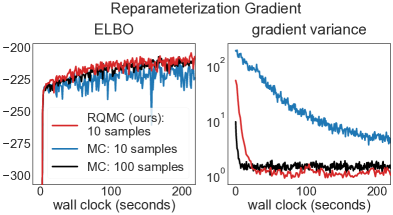
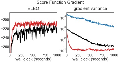
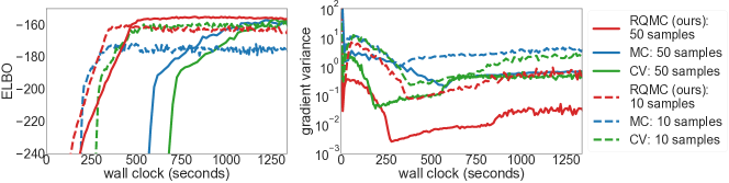
We optimize the elbo using Adam (Kingma and Ba, 2015) based on the score function as well as the reparameterization gradient estimator. We compare the standard mc based approach using 10 and $100$ samples with our rqmc based approach using $10$ samples, respectively. The cv based estimator cannot be used in this setting since it only supports Gaussian variational distributions and the variational family includes a lognormal distribution. For the score function estimator, we set the initial step size of Adam to $0.01$.

The results are shown in Figure 1. We find that using rqmc samples decreases the variance of the gradient estimator substantially. This applies both to the score function and the reparameterization gradient estimator. Our approach substantially improves the standard score function estimator in terms of convergence speed and leads to a decreased gradient variance of up to three orders of magnitude. Our approach is also beneficial in the case of the reparameterization gradient estimator, as it allows for reducing the sample size from 100 mc samples to 10 rqmc samples, yielding a similar gradient variance and optimization speed.

4.2 Multi-level Poisson GLM

We use a multi-level Poisson generalized linear model (GLM), as introduced in (Gelman and Hill, 2006) as an example of multi-level modeling. This model has a $37$-dim posterior, resulting from its hierarchical structure.

As in (Miller et al., 2017), we apply this model to the frisk data set (Gelman et al., 2006) that contains information on the number of stop-and-frisk events within different ethnicity groups. The generative process of the model is described in Appendix C.2. We approximate the posterior by a diagonal Gaussian variational distribution.

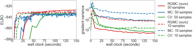
The results are shown in Figure 4. When using a small number of samples $(N=10)$, all three methods have comparable convergence speed and attain a similar optimum. In this setting, the cv based method has lowest gradient variance. When increasing the sample size to $50$, our proposed rqmc approach leads to substantially decreased gradient variance and allows Adam to convergence closer to the optimum than the baselines. This agrees with the fact that rqmc improves over mc for sufficiently large sample sizes.

4.3 Bayesian Neural Network

As a third example, we study qmcvi and its baselines in the context of a Bayesian neural network. The network consists of a $50$-unit hidden layer with ReLU activations. We place a normal prior over each weight, and each weight prior has an inverse Gamma hyper prior. We also place an inverse Gamma prior over the observation variance. The model exhibits a posterior of dimension $d=653$ and is applied to a 100-row subsample of the wine dataset from the UCI repository. The generative process is described in Appendix C.3. We approximate the posterior by a variational diagonal Gaussian.

The results are shown in Figure 4. For $N=10$, both the rqmc and the cv version converge to a comparable value of the elbo, whereas the ordinary mc approach converges to a lower value. For $N=50$, all three algorithms reach approximately the same value of the elbo, but our rqmc method converges much faster. In both settings, the variance of the rqmc gradient estimator is one to three orders of magnitude lower than the variance of the baselines.

4.4 Increasing the Sample Size Over Iterations

Along with our new Monte Carlo variational inference approach qmcvi, Theorem 3 gives rise to a new stochastic optimization algorithm for Monte Carlo objectives. Here, we investigate this algorithm empirically, using a constant learning rate and an (exponentially) increasing sample size schedule. We show that, for strongly convex objective functions and some mild regularity assumptions, our rqmc based gradient estimator leads to a faster asymptotic convergence rate than using the ordinary mc based gradient estimator.

Figure 5: Constant SGD: experiment 4.4. We exemplify the consequences of Theorem 3 and optimize a simple concave elbo using sgd with fixed learning rate $\alpha=0.001$ while the number of samples are iteratively increased. We use an exponential sample size schedule (starting with one sample and 50.000 samples in the final iteration). The logarithmic difference of the elbo to the optimum is plotted. We empirically confirm the result of Theorem 3 and observe a faster asymptotic convergence rate when using rqmc samples over mc samples.

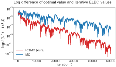
In our experiment, we consider a two-dimensional factorizing normal target distribution with zero mean and standard deviation one. Our variational distribution is also a normal distribution with fixed standard deviation of $1$, and with a variational mean parameter, i.e., we only optimize the mean parameter. In this simple setting, the elbo is strongly convex and the variational family includes the target distribution. We optimize the elbo with an increasing sample size, using the sgd algorithm described in Theorem 3. We initialize the variational parameter to $(0.1,0.1)$. Results are shown in Figure 5.

We considered both rqmc (red) and mc (blue) based gradient estimators. We plot the difference between the optimal elbo value and the optimization trace in logarithmic scale. The experiment confirms the theoretical result of Theorem 3 as our rqmc based method attains a faster asymptotic convergence rate than the ordinary mc based approach. This means that, in the absence of additional noise due to data subsampling, optimizing Monte Carlo objectives with rqmc can drastically outperform sgd.

5 Conclusion

We investigated randomized Quasi-Monte Carlo (rqmc) for stochastic optimization of Monte Carlo objectives. We termed our method Quasi-Monte Carlo Variational Inference (qmcvi), currently focusing on variational inference applications. Using our method, we showed that we can achieve faster convergence due to variance reduction.

qmcvi has strong theoretical guarantees and provably gets us closer to the optimum of the stochastic objective. Furthermore, in absence of additional sources of noise such as data subsampling noise, qmcvi converges at a faster rate than sgd when increasing the sample size over iterations.

qmcvi can be easily integrated into automated inference packages. All one needs to do is replace a sequence of uniform random numbers over the hypercube by an rqmc sequence, and perform the necessary reparameterizations to sample from the target distributions.

An open question remains as to which degree qmcvi can be combined with control variates, as rqmc may introduce additional unwanted correlations between the gradient and the cv. We will leave this aspect for future studies. We see particular potential for qmcvi in the context of reinforcement learning, which we consider to investigate.

Appendix A Additional Information on QMC

We provide some background on qmc sequences that we estimate necessary for the understanding of our algorithm and our theoretical results.

Quasi-Monte Carlo (QMC)

Low discrepancy sequences (also called Quasi Monte Carlo sequences), are used to approximate integrals over the $[0,1]^{d}$ hyper-cube: $\mathbb{E}{\psi(U)}=\int_{[0,1]^{d}}\psi(u)du$, that is the expectation of the random variable $\psi(U)$, where $U\sim\mathcal{U}[0,1]^{d}$, is a uniform distribution on $[0,1]^{d}$. The basic Monte Carlo approximation of the integral is $\hat{I}_{N}:=\frac{1}{N}\sum_{n=1}^{N}\psi(\mathbf{u}_{n})$, where each $\mathbf{u}_{n}\sim\mathcal{U}[0,1]^{d}$, independently. The error of this approximation is $\mathcal{O}(N^{-1})$, since $\operatorname{Var}[\hat{I}_{N}]=\operatorname{Var}[\psi(U)]/N$.

This basic approximation may be improved by replacing the random variables $\mathbf{u}_{n}$ by a low-discrepancy sequence; that is, informally, a deterministic sequence that covers $[0,1]^{d}$ more regularly. The error of this approximation is assessed by the Koksma-Hlawka inequality (Hickernell, 2006):

$$\left|\int_{[0,1]^{d}}\psi(\mathbf{u})d\mathbf{u}-\frac{1}{N}\sum_{n=1}^{N}\psi(\mathbf{u}_{n})\right|\leq V(\psi)D^{*}(\mathbf{u}_{1:N}),$$ (8)

where $V(\psi)$ is the total variation in the sense of Hardy and Krause (Hardy, 1905). This quantity is closely linked to the smoothness of the function $\psi$. $D^{*}(\mathbf{u}_{1:N})$ is called the star discrepancy, that measures how well the sequence covers the target space.

The general notion of discrepancy of a given sequence $\mathbf{u}_{1},\cdots,\mathbf{u}_{N}$ is defined as follows:

$$D(\mathbf{u}_{1:N},\mathcal{A}):=\sup_{A\in\mathcal{A}}\left|\frac{1}{N}\sum_{n=1}^{N}\mathds{1}\left\{\mathbf{u}_{n}\in A\right\}-\lambda_{d}(A)\right|,$$

where $\lambda_{d}(A)$ is the volume (Lebesgue measure on $\mathbb{R}^{d}$) of $A$ and $\mathcal{A}$ is a set of measurable sets. When we fix the sets $A=[0,\mathbf{b}]=\prod_{i=1}^{d}[0,b_{i}]$ with $0\leq b_{i}\leq 1$ as a products set of intervals anchored at $0$, the star discrepancy is then defined as follows

$$D^{*}(\mathbf{u}_{1:N}):=\sup_{[0,\mathbf{b}]}\left|\frac{1}{N}\sum_{n=1}^{N}\mathds{1}\left\{\mathbf{u}_{n}\in[0,\mathbf{b}]\right\}-\lambda_{d}([0,\mathbf{b}])\right|.$$

It is possible to construct sequences such that $D^{*}(\mathbf{u}_{1:N})=\mathcal{O}((\log N)^{2d-2}/N^{2})$. See also Kuipers and Niederreiter (2012) and Leobacher and Pillichshammer (2014) for more details.

Thus, qmc integration schemes are asymptotically more efficient than mc schemes. However, if the dimension $d$ gets too large, the number of necessary samples $N$ in order to reach the asymptotic regime becomes prohibitive. As the upper bound is rather pessimistic, in practice qmc integration outperforms mc integration even for small $N$ in most applications, see e.g. the examples in Chapter 5 of Glasserman (2013). Popular qmc sequences are for example the Halton sequence or the Sobol sequence. See e.g. Dick et al. (2013) for details on the construction. A drawback of qmc is that it is difficult to assess the error and that the deterministic approximation is inherently biased.

Ramdomized Quasi Monte Carlo (RQMC).

The reintroduction of randomness in a low discrepancy sequence while preserving the low discrepancy properties enables the construction of confidence intervals by repeated simulation. Moreover, the randomization makes the approximation unbiased. The simplest method for this purpose is a randomly shifted sequence. Let $v\sim\mathcal{U}[0,1]^{d}$. Then the sequence based on $\hat{\mathbf{u}}_{n}:=\mathbf{u}_{n}+v\mod 1$ preserves the properties of the qmc sequence with probability $1$ and is marginally uniformly distributed.

Scrambled nets (Owen, 1997) represent a more sophisticated approach. Assuming smoothness of the derivatives of the function, Gerber (2015) showed recently, that rates of $\mathcal{O}(N^{-2})$ are achievable. We summarize the best rates in table 1.

MC	QMC	RQMC
$N^{-1}$	$N^{-2}(\log N)^{2d-2}$	$N^{-2}$

Table 1: Best achievable rates for mc, qmc and rqmc in terms of the MSE of the approximation.

Transforming qmc and rqmc sequences

A generic recipe for using qmc / rqmc for integration is given by transforming a sequence with the inverse Rosenblatt transformation $\Gamma:\mathbf{u}\in[0,1]^{d}\mapsto\mathbf{z}\in\mathbb{R}^{d}$, see Rosenblatt (1952) and Gerber and Chopin (2015), such that

$$\int\psi(\Gamma(\mathbf{u}))d\mathbf{u}=\int\psi(\mathbf{z})p(\mathbf{z})d\mathbf{z},$$

where $p(\mathbf{z})$ is the respective measure of integration. The inverse Rosenblatt transformation can be understood as the multivariate extension of the inverse cdf transform. For the procedure to be correct we have to make sure that $\psi\circ\Gamma$ is sufficiently regular.

Theoretical Results on RQMC

In our analysis we mainly use the following result.

Theorem 4

(Owen et al., 2008) Let $\psi:[0,1]^{d}\rightarrow\mathbb{R}$ be a function such that its cross partial derivatives up to order $d$ exist and are continuous, and let $(\mathbf{u}_{n})_{n\in 1:N}$ be a relaxed scrambled $(\alpha,s,m,d)$-net in base $b$ with dimension $d$ with uniformly bounded gain coefficients. Then,

$$\operatorname{Var}\left(\frac{1}{N}\sum_{n=1}^{N}\psi(\mathbf{u}_{n})\right)=\mathcal{O}\left(N^{-3}\log(N)^{(d-1)}\right),$$

where $N=\alpha b^{m}$.

In words, $\forall\tau>0$ the rqmc error rate is $\mathcal{O}(N^{-3+\tau})$ when a scrambled $(\alpha,s,m,d)$-net is used. However, a more general result has recently been shown by Gerber (2015)[Corollary 1], where if $\psi$ is square integrable and $(\mathbf{u}_{n})_{n\in 1:N}$ is a scrambled $(s,d)$-sequence, then

$$\operatorname{Var}\left(\frac{1}{N}\sum_{n=1}^{N}\psi(\mathbf{u}_{n})\right)=o\left(N^{-1}\right).$$

This result shows that rqmc integration is always better than MC integration. Moreover, Gerber (2015)[Proposition 1] shows that rates $\mathcal{O}(N^{-2})$ can be obtained when the function $\psi$ is regular in the sense of Theorem 4 . In particular one gets

$$\operatorname{Var}\left(\frac{1}{N}\sum_{n=1}^{N}\psi(\mathbf{u}_{n})\right)=\mathcal{O}\left(N^{-2}\right).$$

Appendix B Proofs

Our proof are deduced from standard results in the stochastic approximation literature, e.g. Bottou et al. (2016), when the variance of the gradient estimator is reduced due to rqmc sampling. Our proofs rely on scrambled $(s,d)$-sequences in order to use the result of Gerber (2015). The scrambled Sobol sequence, that we use in our simulations satisfies the required properties. We denote by $\mathbb{E}$ the total expectation and by $\mathbb{E}_{U_{N,t}}$ the expectation with respect to the rqmc sequence $U_{N}$ generated at time $t$. Note, that $\mathbf{\lambda}_{t}$ is not a random variable w.r.t. $U_{N,t}$ as it only depends on all the previous $U_{N,1},\cdots,U_{N,t-1}$ due to the update equation in (6). However, $\hat{F}_{N}(\mathbf{\lambda}_{t})$ is a random variable depending on $U_{N,t}$.

B.1 Proof of Theorem 1

Let us first prove that $\operatorname{tr}\operatorname{Var}\left[\hat{g}_{N}(\mathbf{\lambda})\right]\leq M_{V}\times r(N)$ for all $\mathbf{\lambda}$. By assumption we have that $g_{z}(\mathbf{\lambda})$ with $z=\Gamma(\mathbf{u})$ is a function $G:\mathbf{u}\mapsto g_{\Gamma(\mathbf{u})}(\mathbf{\lambda})$ with continuous mixed partial derivatives of up to order $d$ for all $\mathbf{\lambda}$. Therefore, if $\mathbf{u}_{1},\cdots,\mathbf{u}_{N}$ is a rqmc sequence, then the trace of the variance of the estimator $\hat{g}_{N}(\mathbf{\lambda})$ is upper bounded by Theorem 4 and its extension by Gerber (2015)[Proposition 1] by a uniform bound $M_{V}$ and the quantity $r(N)=\mathcal{O}(N^{-2})$, that goes to $0$ faster than the Monte Carlo rate $1/N$.

By the Lipschitz assumption we have that $F(\mathbf{\lambda})\leq F(\overline{\mathbf{\lambda}})+\nabla F(\overline{\mathbf{\lambda}})^{T}(\mathbf{\lambda}-\overline{\mathbf{\lambda}})+\frac{1}{2}L\|\mathbf{\lambda}-\overline{\mathbf{\lambda}}\|^{2}_{2}$, $\forall\mathbf{\lambda},\overline{\mathbf{\lambda}}$, see for example Bottou et al. (2016). By using the fact that $\mathbf{\lambda}_{t+1}-\mathbf{\lambda}_{t}=-\alpha\hat{g}_{N}(\mathbf{\lambda}_{t})$ we obtain

$$F(\mathbf{\lambda}_{t+1})-F(\mathbf{\lambda}_{t})$$

$$\leq \nabla F(\mathbf{\lambda}_{t})^{T}(\mathbf{\lambda}_{t+1}-\mathbf{\lambda}_{t})+\frac{1}{2}L\|\mathbf{\lambda}_{t+1}-\mathbf{\lambda}_{t}\|^{2}_{2},$$

$$= -\alpha\nabla F(\mathbf{\lambda}_{t})^{T}\hat{g}_{N}(\mathbf{\lambda}_{t})+\frac{\alpha^{2}L}{2}\|\hat{g}_{N}(\mathbf{\lambda}_{t})\|^{2}_{2}.$$

After taking expectations with respect to $U_{N,t}$ we obtain

$$\mathbb{E}_{U_{N,t}}F(\mathbf{\lambda}_{t+1})-F(\mathbf{\lambda}_{t})$$

$$\leq -\alpha\nabla F(\mathbf{\lambda}_{t})\mathbb{E}_{U_{N,t}}\hat{g}_{N}(\mathbf{\lambda}_{t})+\frac{\alpha^{2}L}{2}\mathbb{E}_{U_{N,t}}\|\hat{g}_{N}(\mathbf{\lambda}_{t})\|^{2}_{2}.$$

We now use the fact that $\mathbb{E}_{U_{N,t}}\|\hat{g}_{N}(\mathbf{\lambda}_{t})\|^{2}_{2}=\operatorname{tr}\operatorname{Var}_{U_{N,t}}\left[\hat{g}_{N}(\mathbf{\lambda}_{t})\right]+\|\mathbb{E}_{U_{N,t}}\hat{g}_{N}(\mathbf{\lambda}_{t})\|^{2}_{2}$ and after exploiting the fact that $\mathbb{E}_{U_{N,t}}\hat{g}_{N}(\mathbf{\lambda}_{t})=\nabla F(\mathbf{\lambda}_{t})$ we obtain

$$\mathbb{E}_{U_{N,t}}F(\mathbf{\lambda}_{t+1})-F(\mathbf{\lambda}_{t})$$

$$\leq -\alpha\|\nabla F(\mathbf{\lambda}_{t})\|^{2}_{2}+\frac{\alpha^{2}L}{2}\left[\operatorname{tr}\operatorname{Var}_{U_{N,t}}\left[\hat{g}_{N}(\mathbf{\lambda}_{t})\right]+\|\nabla F(\mathbf{\lambda}_{t})\|^{2}_{2}\right],$$

$$= \frac{\alpha^{2}L}{2}\operatorname{tr}\operatorname{Var}_{U_{N,t}}\left[\hat{g}_{N}(\mathbf{\lambda}_{t})\right]+\left(\frac{\alpha^{2}L}{2}-\alpha\right)\|\nabla F(\mathbf{\lambda}_{t})\|^{2}_{2}.$$

The inequality is now summed for $t=1,\cdots,T$ and we take the total expectation:

$$\mathbb{E}F(\mathbf{\lambda}_{T})-F(\mathbf{\lambda}_{1})$$

$$\leq \frac{\alpha^{2}L}{2}\sum_{t=1}^{T}\mathbb{E}\operatorname{tr}\operatorname{Var}_{U_{N,t}}\left[\hat{g}_{N}(\mathbf{\lambda}_{t})\right]$$

$$+\left(\frac{\alpha^{2}L}{2}-\alpha\right)\sum_{t=1}^{T}\mathbb{E}\|\nabla F(\mathbf{\lambda}_{t})\|^{2}_{2}.$$

We use the fact that $F(\mathbf{\lambda}^{\star})-F(\mathbf{\lambda}_{1})\leq\mathbb{E}F(\mathbf{\lambda}_{T})-F(\mathbf{\lambda}_{1})$, where $\mathbf{\lambda}_{1}$ is deterministic and $\mathbf{\lambda}^{\star}$ is the true minimizer, and divide the inequality by $T$:

$$\frac{1}{T}\left[F(\mathbf{\lambda}^{\star})-F(\mathbf{\lambda}_{1})\right]$$

$$\leq \frac{\alpha^{2}L}{2}\frac{1}{T}\sum_{t=1}^{T}\mathbb{E}\operatorname{tr}\operatorname{Var}_{U_{N,t}}\left[\hat{g}_{N}(\mathbf{\lambda}_{t})\right]$$

References

- Antonov and Saleev (1979) Antonov, I. A. and Saleev, V. (1979). An economic method of computing LP-sequences. USSR Computational Mathematics and Mathematical Physics, 19(1):252–256.
- Blei et al. (2017) Blei, D. M., Kucukelbir, A., and McAuliffe, J. D. (2017). Variational inference: A review for statisticians. Journal of the American Statistical Association, 112(518):859–877.
- Bottou et al. (2016) Bottou, L., Curtis, F. E., and Nocedal, J. (2016). Optimization methods for large-scale machine learning. arXiv preprint arXiv:1606.04838.
- Buchholz and Chopin (2017) Buchholz, A. and Chopin, N. (2017). Improving approximate Bayesian computation via quasi Monte Carlo. arXiv preprint arXiv:1710.01057.
- Burda et al. (2016) Burda, Y., Grosse, R., and Salakhutdinov, R. (2016). Importance weighted autoencoders. Proceedings of the International Conference on Learning Representations.
- Carpenter et al. (2017) Carpenter, B., Gelman, A., Hoffman, M., Lee, D., Goodrich, B., Betancourt, M., Brubaker, M., Guo, J., Li, P., and Riddell, A. (2017). Stan: A probabilistic programming language. Journal of Statistical Software, Articles, 76(1):1–32.
- Christophe and Petr (2015) Christophe, D. and Petr, S. (2015). randtoolbox: Generating and Testing Random Numbers. R package version 1.17.
- Defazio et al. (2014) Defazio, A., Bach, F., and Lacoste-Julien, S. (2014). Saga: A fast incremental gradient method with support for non-strongly convex composite objectives. In Advances in Neural Information Processing Systems, pages 1646–1654.
- Dick et al. (2013) Dick, J., Kuo, F. Y., and Sloan, I. H. (2013). High-dimensional integration: The quasi-monte carlo way. Acta Numerica, 22:133–288.
- Drew and Homem-de Mello (2006) Drew, S. S. and Homem-de Mello, T. (2006). Quasi-monte carlo strategies for stochastic optimization. In Proceedings of the 38th conference on Winter simulation, pages 774–782. Winter Simulation Conference.
- Drovandi and Tran (2018) Drovandi, C. C. and Tran, M.-N. (2018). Improving the Efficiency of Fully Bayesian Optimal Design of Experiments Using Randomised Quasi-Monte Carlo. Bayesian Anal., 13(1):139–162.
- Duchi et al. (2011) Duchi, J., Hazan, E., and Singer, Y. (2011). Adaptive subgradient methods for online learning and stochastic optimization. Journal of Machine Learning Research, 12(Jul):2121–2159.
- Gelman and Hill (2006) Gelman, A. and Hill, J. (2006). Data analysis using regression and multilevel/hierarchical models. Cambridge university press.
- Gelman et al. (2006) Gelman, A., Kiss, A., and Fagan, J. (2006). An analysis of the nypd’s stop-and-frisk policy in the context of claims of racial bias. Columbia Public Law & Legal Theory Working Papers, page 0595.
- Gerber (2015) Gerber, M. (2015). On integration methods based on scrambled nets of arbitrary size. Journal of Complexity, 31(6):798–816.
- Gerber and Bornn (2017) Gerber, M. and Bornn, L. (2017). Improving simulated annealing through derandomization. Journal of Global Optimization, 68(1):189–217.
- Gerber and Chopin (2015) Gerber, M. and Chopin, N. (2015). Sequential quasi monte carlo. Journal of the Royal Statistical Society: Series B (Statistical Methodology), 77(3):509–579.
- Glasserman (2013) Glasserman, P. (2013). Monte Carlo methods in financial engineering, volume 53. Springer Science & Business Media.
- Goodfellow et al. (2014) Goodfellow, I., Pouget-Abadie, J., Mirza, M., Xu, B., Warde-Farley, D., Ozair, S., Courville, A., and Bengio, Y. (2014). Generative adversarial nets. In Advances in neural information processing systems, pages 2672–2680.
- Halton (1964) Halton, J. H. (1964). Algorithm 247: Radical-inverse quasi-random point sequence. Communications of the ACM, 7(12):701–702.
- Hardy (1905) Hardy, G. H. (1905). On double Fourier series, and especially those which represent the double zeta-function with real and incommensurable parameters. Quart. J., 37:53–79.
- Hickernell (2006) Hickernell, F. J. (2006). Koksma-Hlawka Inequality. American Cancer Society.
- Hickernell et al. (2005) Hickernell, F. J., Lemieux, C., Owen, A. B., et al. (2005). Control variates for quasi-monte carlo. Statistical Science, 20(1):1–31.
- Hoffman et al. (2013) Hoffman, M. D., Blei, D. M., Wang, C., and Paisley, J. (2013). Stochastic variational inference. The Journal of Machine Learning Research, 14(1):1303–1347.
- Johnson and Zhang (2013) Johnson, R. and Zhang, T. (2013). Accelerating stochastic gradient descent using predictive variance reduction. In Advances in neural information processing systems, pages 315–323.
- Jordan et al. (1999) Jordan, M. I., Ghahramani, Z., Jaakkola, T. S., and Saul, L. K. (1999). An introduction to variational methods for graphical models. Machine learning, 37(2):183–233.
- Joy et al. (1996) Joy, C., Boyle, P. P., and Tan, K. S. (1996). Quasi-monte carlo methods in numerical finance. Management Science, 42(6):926–938.
- Kingma and Ba (2015) Kingma, D. and Ba, J. (2015). Adam: A method for stochastic optimization. Proceedings of the International Conference on Learning Representations.
- Kingma and Welling (2014) Kingma, D. P. and Welling, M. (2014). Auto-encoding variational bayes. Proceedings of the International Conference on Learning Representations.
- Kuipers and Niederreiter (2012) Kuipers, L. and Niederreiter, H. (2012). Uniform distribution of sequences. Courier Corporation.
- L’Ecuyer and Lemieux (2005) L’Ecuyer, P. and Lemieux, C. (2005). Recent advances in randomized quasi-Monte Carlo methods. In Modeling uncertainty, pages 419–474. Springer.
- Lemieux and L’Ecuyer (2001) Lemieux, C. and L’Ecuyer, P. (2001). On the use of quasi-monte carlo methods in computational finance. In International Conference on Computational Science, pages 607–616. Springer.
- Leobacher and Pillichshammer (2014) Leobacher, G. and Pillichshammer, F. (2014). Introduction to quasi-Monte Carlo integration and applications. Springer.
- Mandt et al. (2017) Mandt, S., Hoffman, M. D., and Blei, D. M. (2017). Stochastic Gradient Descent as Approximate Bayesian Inference. Journal of Machine Learning Research, 18(134):1–35.
- Miller et al. (2017) Miller, A. C., Foti, N., D’Amour, A., and Adams, R. P. (2017). Reducing reparameterization gradient variance. In Advances in Neural Information Processing Systems.
- Moulines and Bach (2011) Moulines, E. and Bach, F. R. (2011). Non-asymptotic analysis of stochastic approximation algorithms for machine learning. In Advances in Neural Information Processing Systems.
- Nesterov (2013) Nesterov, Y. (2013). Introductory lectures on convex optimization: A basic course, volume 87. Springer Science & Business Media.
- Niederreiter (1992) Niederreiter, H. (1992). Random number generation and quasi-Monte Carlo methods. SIAM.
- Oates and Girolami (2016) Oates, C. and Girolami, M. (2016). Control functionals for quasi-monte carlo integration. In Artificial Intelligence and Statistics, pages 56–65.
- Oates et al. (2017) Oates, C. J., Girolami, M., and Chopin, N. (2017). Control functionals for Monte Carlo integration. Journal of the Royal Statistical Society: Series B (Statistical Methodology), 79(3):695–718.
- Owen (1997) Owen, A. B. (1997). Scrambled Net Variance for Integrals of Smooth Functions. The Annals of Statistics, 25(4):1541–1562.
- Owen et al. (2008) Owen, A. B. et al. (2008). Local antithetic sampling with scrambled nets. The Annals of Statistics, 36(5):2319–2343.
- Paisley et al. (2012) Paisley, J., Blei, D., and Jordan, M. (2012). Variational Bayesian inference with stochastic search. International Conference on Machine Learning.
- Ranganath et al. (2014) Ranganath, R., Gerrish, S., and Blei, D. M. (2014). Black box variational inference. In Proceedings of the International Conference on Artificial Intelligence and Statistics.
- Rezende et al. (2014) Rezende, D. J., Mohamed, S., and Wierstra, D. (2014). Stochastic backpropagation and approximate inference in deep generative models. In Proceedings of the International Conference on Machine Learning.
- Robbins and Monro (1951) Robbins, H. and Monro, S. (1951). A stochastic approximation method. The annals of mathematical statistics, pages 400–407.
- Robert and Casella (2013) Robert, C. and Casella, G. (2013). Monte Carlo Statistical Methods. Springer Science & Business Media.
- Roeder et al. (2017) Roeder, G., Wu, Y., and Duvenaud, D. K. (2017). Sticking the landing: Simple, lower-variance gradient estimators for variational inference. In Advances in Neural Information Processing Systems.
- Rosenblatt (1952) Rosenblatt, M. (1952). Remarks on a multivariate transformation. Ann. Math. Statist., 23(3):470–472.
- Ruiz et al. (2016a) Ruiz, F. J. R., Titsias, M. K., and Blei, D. M. (2016a). Overdispersed black-box variational inference. In Proceedings of the Conference on Uncertainty in Artificial Intelligence.
- Ruiz et al. (2016b) Ruiz, F. R., Titsias, M., and Blei, D. (2016b). The generalized reparameterization gradient. In Advances in Neural Information Processing Systems.
- Sutton and Barto (1998) Sutton, R. S. and Barto, A. G. (1998). Reinforcement learning: An introduction. MIT press Cambridge.
- Tran et al. (2016) Tran, D., Kucukelbir, A., Dieng, A. B., Rudolph, M., Liang, D., and Blei, D. M. (2016). Edward: A library for probabilistic modeling, inference, and criticism. arXiv preprint arXiv:1610.09787.
- Tran et al. (2017) Tran, M.-N., Nott, D. J., and Kohn, R. (2017). Variational bayes with intractable likelihood. Journal of Computational and Graphical Statistics, 26(4):873–882.
- Yang et al. (2014) Yang, J., Sindhwani, V., Avron, H., and Mahoney, M. (2014). Quasi-monte carlo feature maps for shift-invariant kernels. In International Conference on Machine Learning, pages 485–493.
- Zhang et al. (2017a) Zhang, C., Butepage, J., Kjellstrom, H., and Mandt, S. (2017a). Advances in variational inference. arXiv preprint arXiv:1711.05597.
- Zhang et al. (2017b) Zhang, C., Kjellström, H., and Mandt, S. (2017b). Determinantal point processes for mini-batch diversification. In Uncertainty in Artificial Intelligence, UAI 2017.