Realistic compactification in spatially flat vacuum cosmological models in cubic Lovelock gravity: High-dimensional case

Abstract

In this paper we perform systematic investigation of all possible regimes in spatially flat vacuum cosmological models in cubic Lovelock gravity. The spatial section is considered as a product of three- and extra-dimensional isotropic subspaces, and the former represents our Universe. As the equations of motion are different for $D=3,4,5$ and general $D\geqslant 6$ cases, we considered them all separately. This is the second paper of the series, and we consider $D=5$ and general $D\geqslant 6$ cases here. For each $D$ case we found critical values for $\alpha$ (Gauss-Bonnet coupling) and $\beta$ (cubic Lovelock coupling) which separate different dynamical cases, isotropic and anisotropic exponential solutions, and study the dynamics in each region to find all regimes for all initial conditions and for arbitrary values of $\alpha$ and $\beta$. The results suggest that in all $D\geqslant 3$ there are regimes with realistic compactification originating from so-called “generalized Taub” solution. The endpoint of the compactification regimes is either anisotropic exponential solution (for $\alpha>0$, $\mu\equiv\beta/\alpha^{2}<\mu_{1}$ (including entire $\beta<0$)) or standard Kasner regime (for $\alpha>0$, $\mu>\mu_{1}$). For $D\geqslant 8$ there is additional regime which originates from high-energy (cubic Lovelock) Kasner regime and ends as anisotropic exponential solution. It exists in two domains: $\alpha>0$, $\beta<0$, $\mu\leqslant\mu_{4}$ and entire $\alpha>0$, $\beta>0$. Let us note that for $D\geqslant 8$ and $\alpha>0$, $\beta<0$, $\mu<\mu_{4}$ there are two realistic compactification regimes which exist at the same time and have two different anisotropic exponential solutions as a future asymptotes. For $D\geqslant 8$ and $\alpha>0$, $\beta>0$, $\mu<\mu_{2}$ there are two realistic compactification regimes but they lead to the same anisotropic exponential solution. This behavior is quite different from the Einstein-Gauss-Bonnet case. There are two more unexpected observations among the results – all realistic compactification regimes exist only for $\alpha>0$ and there is no smooth transition from high-energy Kasner regime to the low-energy regime with realistic compactification.

I Introduction

It is not widely known but the idea of extra dimensions is older then General Relativity (GR) itself. Indeed, the first known extra-dimensional model was introduced by Nordström in 1914 Nord1914 – it unified Nordström’s second gravity theory Nord_2grav with Maxwell’s electromagnetism. Soon after that Einstein proposed GR einst , but it took years before it was accepted: during the solar eclipse of 1919, the bending of light near the Sun was measured and the deflection angle was in perfect agreement with GR, while Nordström’s theory predicted a zeroth deflection angle, as most of the scalar gravity theories do.

But the idea of extra dimensions was not forgotten – in 1919 Kaluza proposed KK1 a very similar model but based on GR: in his model five-dimensional Einstein equations are decomposed into $4D$ Einstein equations and Maxwell’s electromagnetism. But for such decomposition to exist, the extra dimensions should be “curled” or compactified into a circle and “cylindrical conditions” should be imposed. The work by Kaluza was followed by Klein who proposed KK2 ; KK3 a nice quantum mechanical interpretation of this extra dimension and so the theory, called Kaluza-Klein after its founders, was finalized. It is interesting to note that their theory unified all known interactions at their time. With flow of time, more interactions were discovered and it became clear that to unify all of them, more extra dimensions are needed. At present, one of the promising theories to unify all interactions is M/string theory.

One of the distinguishing features of M/string theories is the presence in the Lagrangian of the corrections which are quadratic in curvature. Scherk and Schwarz sch-sch demonstrated that $R^{2}$ and $R_{\mu\nu}R^{\mu\nu}$ terms are presented in the Lagrangian of the Virasoro-Shapiro model VSh1 ; VSh2 ; presence of the term of $R^{\mu\nu\lambda\rho}R_{\mu\nu\lambda\rho}$ type was found in Candelas_etal for the low-energy limit of the $E_{8}\times E_{8}$ heterotic superstring theory Gross_etal to match the kinetic term of the Yang-Mills field. Later Zwiebach demonstrated zwiebach that the only combination of quadratic terms that leads to a ghost-free nontrivial gravitation interaction is the Gauss-Bonnet (GB) term:

$$L_{GB}=L_{2}=R_{\mu\nu\lambda\rho}R^{\mu\nu\lambda\rho}-4R_{\mu\nu}R^{\mu\nu}+R^{2}.$$

This term was first discovered by Lanczos Lanczos1 ; Lanczos2 (and so sometimes it is referred to as the Lanczos term), is an Euler topological invariant in (3+1)-dimensional space-time, but in (4+1) and higher dimensions it gives nontrivial contribution to the equations of motion. Zumino zumino extended Zwiebach’s result on the higher-order curvature terms, supporting the idea that the low-energy limit of the unified theory might have a Lagrangian density as a sum of contributions of different powers of curvature. The sum of all possible Euler topological invariants, which give nontrivial contribution to the equations of motion in a particular number of space-time dimensions, form more general Lovelock gravity Lovelock .

When someone mention extra spatial dimensions, the natural question arises – where they are? Our everyday experience clearly points on three spatial dimensions, and experiments in physics and theory support this (for example, in Newtonian gravity if there are more then three space dimensions, no stable orbits exist, while we clearly see they do). The string theorists working with extra dimensions proposed an answer – the extra spatial dimensions are compact – they are compactified on a very small scale, so small that we cannot sense them with our level of equipment. But with an answer like that, another natural question comes to mind – how come that they are compact? The answer to this question is not that simple. One of the ways to hide extra dimensions and to recover four-dimensional physics, is so-called “spontaneous compactification”. Exact static solutions of this type with the metric as a cross product of a (3+1)-dimensional Minkowski space-time and a constant curvature “inner space”, were found for the first time in add_1 (the generalization for a constant curvature Lorentzian manifold was done in Deruelle2 ). For cosmology, it is more useful to consider the four-dimensional space-time given by a Friedmann-Robertson-Walker metric, and the size of extra dimensions to be time-dependent rather then static. In add_4 it was demonstrated that to have a more realistic model it is necessary to consider the dynamical evolution of the extra-dimensional scale factor. In Deruelle2 , the equations of motion with time-dependent scale factors were written for arbitrary Lovelock order in the special case of a spatially flat metric (the results were further proven and extended in prd09 ). The results of Deruelle2 were further analyzed for the special case of 10 space-time dimensions in add_10 . In add_8 , the dynamical compactification was studied with use of the Hamiltonian formalism. More recently, studies of the spontaneous compactifications were made in add13 , where the dynamical compactification of the (5+1) Einstein-Gauss-Bonnet (EGB) model was considered; in MO04 ; MO14 with different metric Ansätze for scale factors corresponding to (3+1)- and extra-dimensional parts. Also, apart from the cosmology, the recent analysis was focused on properties of black holes in Gauss-Bonnet alpha_12 ; add_rec_1 ; add_rec_2 ; addn_1 ; addn_2 ; add_o_1 ; add_o_2 ; add_o_3 and Lovelock add_rec_3 ; add_rec_4 ; addn_3 ; addn_4 ; addn_4.1 gravities, features of gravitational collapse in these theories addn_5 ; addn_6 ; addn_7 , general features of spherical-symmetric solutions addn_8 , and many others.

If we want to find exact cosmological solutions, the most common Ansatz for the scale factor is either exponential or power-law. Exact solutions with exponents for both the (3+1)- and extra-dimensional scale factors were studied for the first time in Is86 , and exponentially expanding (3+1)-dimensional part and an exponentially shrinking extra-dimensional scale factor were described. Power-law solutions have been considered in Deruelle1 ; Deruelle2 and more recently in mpla09 ; prd09 ; Ivashchuk ; prd10 ; grg10 so that by now there is more-or-less complete description of the solutions of this kind (see also PT for comments regarding different physical branches of the power-law solutions). Solutions with exponential scale factors KPT have also been studied in detail, namely, the models with both variable CPT1 and constant CST2 volume; the general scheme for finding anisotropic exponential solutions in EGB gravity was developed and generalized for general Lovelock gravity of any order and in any dimensions CPT3 . The stability of the exponential solutions was addressed in my15 (see also iv16 for stability of general exponential solutions in EGB gravity), and it was demonstrated that only a handful of the solutions found and described in CPT3 could be called “stable”, while the most of them are either unstable or have neutral/marginal stability.

In order to find all possible cosmological regimes in EGB gravity, one needs to go beyond an exponential or power-law Ansatz and keep the scale factor generic. We are especially interested in models that allow dynamical compactification, so that we consider the metric to be the product of a spatially three-dimensional and extra-dimensional parts. In that case the three-dimensional part is “our Universe” and we expect for this part to expand while the extra-dimensional part should be suppressed in size with respect to the three-dimensional one. In CGP1 we demonstrated the there exist the phenomenologically sensible regime when the curvature of the extra dimensions is negative and the EGB theory does not admit a maximally-symmetric solution. In this case both the three-dimensional Hubble parameter and the extra-dimensional scale factor asymptotically tend to the constant values. In CGP2 we continued investigation of this case and performed a detailed analysis of the cosmological dynamics in this model with generic couplings. Recent analysis of this model CGPT revealed that, with an additional constraint on couplings, Friedmann-type late-time behavior could be restored.

With the exponential and power-law solutions described in the mentioned above papers, another natural question arise – could these solutions describe realistic compactification (i.e., with proper both past and future asymptotes) or are they just solutions with no connection to the reality? To answer this question, we have considered the cosmological model in EGB gravity with the spatial part being the product of three- and extra dimensional parts with both subspaces being spatially flat. As both subspaces are spatially flat, we can rewrite the equations of motion in terms of Hubble parameters, so that they become first order differential equations and could be analytically analyzed to find all possible regimes, asymptotes, exponential and power-law solutions. For vacuum EGB model it was done in my16a and reanalyzed in my18a . The results suggest that the vacuum model has two physically viable regimes – first of them is the smooth transition from high-energy GB Kasner (or generalized Taub solution) to low-energy GR Kasner. This regime exists for $\alpha>0$ (Gauss-Bonnet coupling) at $D=1,\,2$ (the number of extra dimensions) and for $\alpha<0$ at $D\geqslant 2$ (so that at $D=2$ it appears for both signs of $\alpha$). Another viable regime is the smooth transition from high-energy GB Kasner to anisotropic exponential solution with expanding three-dimensional section (“our Universe”) and contracting extra dimensions; this regime occurs only for $\alpha>0$ and at $D\geqslant 2$.

The same analysis but for EGB model with $\Lambda$-term was performed in my16b ; my17a and reanalyzed in my18a . The results suggest that the only realistic regime is the transition from high-energy GB Kasner to anisotropic exponential solution, it requires $D\geqslant 2$, see my16b ; my17a ; my18a for exact limits on ($\alpha,\Lambda$) in each particular $D$. The low-energy GR Kasner is forbidden in the presence of the $\Lambda$-term so the corresponding transition does not occur.

In these studies we have made two important assumptions – we considered both subspaces being isotropic and spatially flat. But what will happens in we lift these conditions? Indeed, the spatial section being a product of two isotropic spatially-flat subspaces could hardly be called “natural”, so that we considered the effects of anisotropy and spatial curvature in PT2017 . The initial anisotropy affects the results greatly – indeed, say, in vacuum $(4+1)$-dimensional EGB gravity with Bianchi-I-type metric (all the directions are independent) the only future asymptote is nonstandard singularity prd10 . Our analysis PT2017 suggest that the transition from Gauss-Bonnet Kasner regime to anisotropic exponential expansion (with expanding three and contracting extra dimensions) is stable with respect to breaking the symmetry within both three- and extra-dimensional subspaces. However, the details of the dynamics in $D=2$ and $D\geqslant 3$ are different – in the latter there exist anisotropic exponential solutions with “wrong” spatial splitting and all of them are accessible from generic initial conditions. For instance, in $(6+1)$-dimensional space-time there are anisotropic exponential solutions with $[3+3]$ and $[4+2]$ spatial splittings, and some of the initial conditions in the vicinity of $E_{3+3}$ actually end up in $E_{4+2}$ – the exponential solution with four and two isotropic subspaces. In other words, generic initial conditions could easily end up with “wrong” compactification, giving “wrong” number of expanding spatial dimensions (see PT2017 for details).

The effect of the spatial curvature on the cosmological dynamics also could be dramatic – say, positive curvature changes the inflationary asymptotic infl1 ; infl2 . In the case of EGB gravity the influence of the spatial curvature reveal itself only if the curvature of the extra dimensions is negative and $D\geqslant 3$ – in that case there exist “geometric frustration” regime, described in CGP1 ; CGP2 and further investigated in CGPT . Full investigation of the spatial curvature effects on the existing regimes could be found in PT2017 .

The current manuscript is a direct continuation of my18b , where the same analysis was performed for low-$D$ ($D=3,4$) cases. It also could be called a spiritual successor of my16a ; my16b ; my17a ; my18a – now we are performing the same analysis but for cubic Lovelock gravity. In this paper we consider only vacuum case, $\Lambda$-term case, as well as possible influence of anisotropy, spatial curvature and different kinds of matter source are to be considered in the papers to follow.

The manuscript is structured as follows: first we introduce Lovelock gravity and derive the equations of motion in the general form for the spatially-flat (Bianchi-I-type) metrics. Then we add our Ansatz and write down simplified equations. After that we describe the scheme we are going to use and give some important comments on the existing regimes. After that we consider particular cases with $D=5$ and general $D\geqslant 6$ number of extra dimensions. In each section, dedicated to the particular case, we describe it and briefly summarize its features. Finally we summarize all the cases, discuss their differences and similarities, and describe the effect of $D$ on the features. After that we compare the dynamics in this cubic Lovelock with the dynamics in quadratic Lovelock (Einstein-Gauss-Bonnet) case, described in my16a ; my18a . At last, we draw conclusions and formulate perspective directions for further investigations.

II Equations of motion

Lovelock gravity Lovelock has the following structure: its Lagrangian is constructed from terms

$$L_{n}=\frac{1}{2^{n}}\delta^{i_{1}i_{2}\dots i_{2n}}_{j_{1}j_{2}\dots j_{2n}}R^{j_{1}j_{2}}_{i_{1}i_{2}}\dots R^{j_{2n-1}j_{2n}}_{i_{2n-1}i_{2n}},$$ (1)

where $\delta^{i_{1}i_{2}\dots i_{2n}}_{j_{1}j_{2}\dots j_{2n}}$ is the generalized Kronecker delta of the order $2n$. One can verify that $L_{n}$ is Euler invariant in $\mathcal{D}<2n$ spatial dimensions and so it does not give nontrivial contribution into the equations of motion. Then the Lagrangian density for any given $\mathcal{D}$ spatial dimensions is sum of all Lovelock invariants (1) upto $n=\left[\displaystyle\frac{\mathcal{D}}{2}\right]$ which give nontrivial contributions into equations of motion:

$${\cal L}=\sqrt{-g}\sum_{n}c_{n}L_{n},$$ (2)

where $g$ is the determinant of metric tensor, $c_{n}$ are coupling constants of the order of Planck length in $\mathcal{D}$ dimensions and we assume summation over all $n$ in consideration. The metric ansatz has the form

$$g_{\mu\nu}=\mathop{\rm diag}\nolimits\{-1,a_{1}^{2}(t),a_{2}^{2}(t),\ldots,a_{n}^{2}(t)\}.$$ (3)

As we mentioned, we are interested in the dynamics in cubic Lovelock gravity, so we consider $n$ up to three ($n=0$ is the boundary term while $n=1$ is Einstein-Hilbert, $n=2$ is Gauss-Bonnet and $n=3$ is cubic Lovelock contributions). Substituting metric (3) into the Lagrangian and following the standard procedure gives us the equations of motion:

$$\begin{array}[]{l}2\left[\sum\limits_{j\neq i}(\dot{H}_{j}+H_{j}^{2})+\sum\limits_{\begin{subarray}{c}\{k>l\}\\ \neq i\end{subarray}}H_{k}H_{l}\right]+8\alpha\left[\sum\limits_{j\neq i}(\dot{H}_{j}+H_{j}^{2})\sum\limits_{\begin{subarray}{c}\{k>l\}\\ \neq\{i,j\}\end{subarray}}H_{k}H_{l}+3\sum\limits_{\begin{subarray}{c}\{k>l>\\ m>n\}\neq i\end{subarray}}H_{k}H_{l}H_{m}H_{n}\right]+\\ \\ +144\beta\left[\sum\limits_{j\neq i}(\dot{H}_{j}+H_{j}^{2})\sum\limits_{\begin{subarray}{c}\{k>l>m>\\ n\}\neq\{i,j\}\end{subarray}}H_{k}H_{l}H_{m}H_{n}+5\sum\limits_{\begin{subarray}{c}\{k>l>m>\\ n>p>q\}\neq i\end{subarray}}H_{k}H_{l}H_{m}H_{n}H_{p}H_{q}\right]-\Lambda=0\end{array}$$ (4)

as the $i$th dynamical equation. The first Lovelock term—the Einstein-Hilbert contribution—is in the first set of brackets, the second term—Gauss-Bonnet—is in the second set and the third – cubic Lovelock term—is in the third set; $\alpha$ is the coupling constant for the Gauss-Bonnet contribution while $\beta$ is the coupling constant for cubic Lovelock; we put the corresponding constant for Einstein-Hilbert contribution to unity. Since we consider spatially flat cosmological models, scale factors do not hold much physical sense and the equations are rewritten in terms of the Hubble parameters $H_{i}=\dot{a}_{i}(t)/a_{i}(t)$. Apart from the dynamical equations, we write down the constraint equation

$$\begin{array}[]{l}2\sum\limits_{i>j}H_{i}H_{j}+24\alpha\sum\limits_{\begin{subarray}{c}i>j>\\ k>l\end{subarray}}H_{i}H_{j}H_{k}H_{l}+720\beta\sum\limits_{\begin{subarray}{c}i>j>k\\ >l>m>n\end{subarray}}H_{i}H_{j}H_{k}H_{l}H_{m}H_{n}=\Lambda.\end{array}$$ (5)

As we mentioned in the Introduction, we want to investigate the particular case with the scale factors split into two parts – separately three dimensions (three-dimensional isotropic subspace), which are supposed to represent our Universe, and the remaining represent the extra dimensions ($D$-dimensional isotropic subspace). So we put $H_{1}=H_{2}=H_{3}=H$ and $H_{4}=\ldots=H_{D+3}=h$ ($D$ designs the number of additional dimensions) and the equations take the following form: the dynamical equation that corresponds to $H$,

$$\begin{array}[]{l}2\left[2\dot{H}+3H^{2}+D\dot{h}+\displaystyle\frac{D(D+1)}{2}h^{2}+2DHh\right]+8\alpha\left[2\dot{H}\left(DHh+\displaystyle\frac{D(D-1)}{2}h^{2}\right)+\right.\\ \\ \left.+D\dot{h}\left(H^{2}+2(D-1)Hh+\displaystyle\frac{(D-1)(D-2)}{2}h^{2}\right)+2DH^{3}h+\displaystyle\frac{D(5D-3)}{2}H^{2}h^{2}+\right.\\ \\ \left.+D^{2}(D-1)Hh^{3}+\displaystyle\frac{(D+1)D(D-1)(D-2)}{8}h^{4}\right]+\\ \\ +144\beta\left[\dot{H}\left(Hh^{3}\displaystyle\frac{D(D-1)(D-2)}{3}+h^{4}\displaystyle\frac{D(D-1)(D-2)(D-3)}{12}\right)+\right.\\ \\ +\left.D\dot{h}\left(H^{2}h^{2}\displaystyle\frac{(D-1)(D-2)}{2}+Hh^{3}\displaystyle\frac{(D-1)(D-2)(D-3)}{3}+\right.\right.\\ \\ +\left.\left.h^{4}\displaystyle\frac{(D-1)(D-2)(D-3)(D-4)}{24}\right)+H^{3}h^{3}\displaystyle\frac{D(D-1)(D-2)}{3}+\right.\\ \\ +\left.H^{2}h^{4}\displaystyle\frac{D(D-1)(D-2)(7D-9)}{24}+Hh^{5}\displaystyle\frac{D^{2}(D-1)(D-2)(D-3)}{12}+\right.\\ \\ +\left.h^{6}\displaystyle\frac{(D+1)D(D-1)(D-2)(D-3)(D-4)}{144}\right]-\Lambda=0,\end{array}$$ (6)

the dynamical equation that corresponds to $h$,

$$\begin{array}[]{l}2\left[3\dot{H}+6H^{2}+(D-1)\dot{h}+\displaystyle\frac{D(D-1)}{2}h^{2}+3(D-1)Hh\right]+8\alpha\left[3\dot{H}\left(H^{2}+\right.\right.\\ \\ \left.\left.+2(D-1)Hh+\displaystyle\frac{(D-1)(D-2)}{2}h^{2}\right)+(D-1)\dot{h}\left(3H^{2}+3(D-2)Hh+\right.\right.\\ \\ \left.\left.+\displaystyle\frac{(D-2)(D-3)}{2}h^{2}\right)+3H^{4}+9(D-1)H^{3}h+3(D-1)(2D-3)H^{2}h^{2}+\right.\\ \\ \left.+\displaystyle\frac{3(D-1)^{2}(D-2)}{2}Hh^{3}+\displaystyle\frac{D(D-1)(D-2)(D-3)}{8}h^{4}\right]+\\ \\ +144\beta\left[\dot{H}\left(H^{2}h^{2}\displaystyle\frac{3(D-1)(D-2)}{2}+Hh^{3}(D-1)(D-2)(D-3)+\right.\right.\\ \\ +\left.\left.h^{4}\displaystyle\frac{(D-1)(D-2)(D-3)(D-4)}{8}\right)+(D-1)\dot{h}\left(H^{3}h(D-2)+\right.\right.\\ \\ +\left.\left.H^{2}h^{2}\displaystyle\frac{3(D-2)(D-3)}{2}+Hh^{3}\displaystyle\frac{(D-2)(D-3)(D-4)}{2}+\right.\right.\\ \\ \left.\left.+h^{4}\displaystyle\frac{(D-2)(D-3)(D-4)(D-5)}{24}\right)+H^{4}h^{2}\displaystyle\frac{3(D-1)(D-2)}{2}+\right.\\ \\ \left.+H^{3}h^{3}\displaystyle\frac{(D-1)(D-2)(11D-27)}{6}+H^{2}h^{4}\displaystyle\frac{3(D-1)(D-2)^{2}(D-3)}{4}+\right.\\ \\ \left.+Hh^{5}\displaystyle\frac{(D+1)(D-1)(D-2)(D-3)(D-4)}{12}+\right.\\ \\ \left.+h^{6}\displaystyle\frac{D(D-1)(D-2)(D-3)(D-4)(D-5)}{144}\right]-\Lambda=0,\end{array}$$ (7)

and the constraint equation,

$$\begin{array}[]{l}2\left[3H^{2}+3DHh+\displaystyle\frac{D(D-1)}{2}h^{2}\right]+24\alpha\left[DH^{3}h+\displaystyle\frac{3D(D-1)}{2}H^{2}h^{2}+\right.\\ \\ \left.+\displaystyle\frac{D(D-1)(D-2)}{2}Hh^{3}+\displaystyle\frac{D(D-1)(D-2)(D-3)}{24}h^{4}\right]+720\beta\left[H^{3}h^{3}\displaystyle\frac{D(D-1)(D-2)}{6}+\right.\\ \\ \left.+H^{2}h^{4}\displaystyle\frac{D(D-1)(D-2)(D-3)}{8}+Hh^{5}\displaystyle\frac{D(D-1)(D-2)(D-3)(D-4)}{40}+\right.\\ \\ \left.+h^{6}\displaystyle\frac{D(D-1)(D-2)(D-3)(D-4)(D-5)}{720}\right]=\Lambda.\end{array}$$ (8)

Looking at (6)–(8) one can notice that the structure of the equations depends on the number of extra dimensions $D$ (terms with $(D-4)$ multiplier nullifies in $D=4$ and so on). In previous papers, dedicated to study cosmological dynamics in EGB gravity, we performed analysis in all dimensions, sensitive to EGB case my16a ; my16b ; my17a ; my18a . In the cubic Lovelock, the structure of the equations of motion is different in $D=3,4,5$ and in the general $D\geqslant 6$ cases. In the directly previous paper my18b we performed the analysis for $D=3$ and $D=4$ cases, leaving $D=5$ and the general $D\geqslant 6$ cases for this paper. Also, similar to my18b , since the these papers are dedicated to the vacuum case, we have $\Lambda\equiv 0$.

III General scheme

The procedure of the analysis is exactly the same as described in our previous papers my16a ; my16b ; my17a ; my18a . In the directly previous paper my18b this scheme is described in great detail for $D=3$ case. In the current paper we just list the scheme and use it with almost no details. So the scheme is as follows:

• we solve (8) with respect to $H$ – one can see that it is cubic with respect to $H$ and sixth order with respect to $h$, so that to have analytical solutions, we solve it for $H$; and as a result we have three branches $H_{1}$, $H_{2}$ and $H_{3}$. In lower-dimensional cases we wrote down solutions explicitly, but in higher dimensions they become quite bulky, so we draw $H(h)$ curves instead. If we take the discriminant of (8) with respect to $H$, and then its discriminant with respect to $h$, we obtain critical values for $(\alpha,\beta)$ which separate qualitatively different cases;

• we find analytically isotropic exponential solutions: we substitute $\dot{H}=\dot{h}\equiv 0$ as well as $h=H$ into (6)–(8); the system simplifies into a single equation, we solve it and find not only roots but also the ranges of $(\alpha,\beta)$ where they exist;

• we find analytically anisotropic exponential solutions: we substitute $\dot{H}=\dot{h}\equiv 0$ into (6)–(8); the system could be brought down to two equations: bi-six order polynomial in $h$ with powers of $\alpha$ and $\beta$ as coefficients and $H=H(h,\alpha,\beta)$. Both of them are usually higher-order with respect to their arguments so retrieving the solutions in radicand is impossible. But if we consider the discriminant of the former of them, the resulting equation gives us critical values for $(\alpha,\beta)$ which separate areas with different number of roots;

• first three steps provides us with a set of critical values for $(\alpha,\beta)$ which separate domains with different dynamics;

• we solve (6)–(7) with respect to $\dot{H}$ and $\dot{h}$;

• we substitute obtained $H_{i}$ into $\dot{H}$ and $\dot{h}$ and obtain the latter as a single-variable functions: $\dot{H}(h)$ and $\dot{h}(h)$;

• the obtained $\dot{H}(h)$ and $\dot{h}(h)$ expressions and graphs are analyzed for all possible domains in $(\alpha,\beta)$ space to obtain all possible regimes;

• obtained exponential regimes are compared with exact isotropic and anisotropic solutions (see CPT3 ) to find the nature of the exponential regimes in question;

• power-law regimes are analyzed in terms of Kasner exponents ($p_{i}=-H_{i}^{2}/\dot{H}_{i}$) to verify that low-energy power-law regimes are standard Kasner regimes with $\sum p_{i}=\sum p_{i}^{2}=1$ or “generalized Taub” regimes (see below) while high-energy power-law regimes are Lovelock Kasner regimes with $\sum p_{i}=(2n-1)=5$.

The above scheme allows us to completely describe all existing regimes for a given set of the parameters $(\alpha,\beta)$. In the previous paper my18b we followed the scheme in great detail for $D=3$ case, with full description of all steps, and in the current papers we just briefly mentioned the details and mainly focus on the results.

Before proceeding with the particular cases, it is useful to introduce the notations we are going to use through the paper. We denote Kasner regime as $K_{i}$ where $i$ is the total expansion rate in terms of the Kasner exponents $\sum p_{i}=(2n-1)$ where $n$ is the corresponding order of the Lovelock contribution (see, e.g., prd09 ). So that for Einstein-Hilbert contribution $n=1$ and $\sum p_{i}=1$ (see kasner ) and the corresponding regime is $K_{1}$, which is usual low-energy regime in vacuum EGB case (see my16a ; my18a ) and we expect it to remain here. For Gauss-Bonnet $n=2$ and so $\sum p_{i}=3$ and the regime $K_{3}$ is typical high-energy regime for EGB case (again, see my16a ; my16b ; my17a ; my18a ). Finally, for cubic Lovelock $n=3$ and so $\sum p_{i}=5$ and the regime $K_{5}$ is typical high-energy regime for this case in low $D$ case my18b .

Another power-law regime is what is called “generalized Taub” (see Taub for the original solution). We mistakenly taken it for $K_{3}$ in my16a , but then in my18a corrected ourselves and explained the details (they both have $\sum p_{i}=3$ which causes misinterpreting). It is a situation when for one of the subspaces the Kasner exponent $p$ is equal to zero and for another – to unity. So we denote $P_{1,0}$ the case with $p_{H}=1,p_{h}=0$ and $P_{0,1}$ the case with $p_{H}=0,p_{h}=1$.

The exponential solutions are denoted as $E$ with subindex indicating its details – $E_{iso}$ is isotropic exponential solution and $E_{3+D}$ is anisotropic – with different Hubble parameters corresponding to three- and extra-dimensional subspaces. But in practice, in each particular case there are several different anisotropic exponential solutions, so that instead of using $E_{3+D}$ we use $E_{i}$ where $i$ counts the number of the exponential solution ($E_{1}$, $E_{2}$ etc). In case if there are several isotropic exponential solutions, we count them with upper index: $E_{iso}^{1}$, $E_{iso}^{2}$ etc.

And last but not least regime is what we call “nonstandard singularity” and denote it is as $nS$. It is the situation which arise in Lovelock gravity due to its nonlinear nature. Since the equations (6)–(7) are nonlinear with respect to the highest derivative ($\dot{H}$ and $\dot{h}$ in our case), when we solve them, the resulting expressions are ratios with polynomials in both numerator and denominator. So there exist a situation when the denominator is equal to zero for finite values of $H$ andor $h$. This situation is singular, as the curvature invariants diverge, but it happening for finite values of $H$ andor $h$. Tipler Tipler call this kind of singularity as “weak” while Kitaura and Wheeler KW1 ; KW2 – as “type II”. Our previous research demonstrate that this kind of singularity is widely spread in EGB cosmology – in particular, in totally anisotropic (Bianchi-I-type) $(4+1)$-dimensional vacuum cosmological model it is the only future asymptote prd10 .

IV $D=5$ case

In this case the equations of motion (6)–(8) take form ($H$-equation, $h$-equation, and constraint correspondingly)

$$\begin{array}[]{l}4\dot{H}+6H^{2}+10\dot{h}+30h^{2}+20Hh+8\alpha\left(2\dot{H}(5Hh+10h^{2})+5\dot{h}(H^{2}+6h^{2}+8Hh)+\right.\\ \left.+10H^{3}h+55H^{2}h^{2}+100Hh^{3}+45h^{4}\right)+144\beta\left(2(\dot{H}+H^{2})(10Hh^{3}+5h^{4})+\right.\\ \left.+5(\dot{h}+h^{2})(6H^{2}h^{2}+8Hh^{3}+h^{4})+25H^{2}h^{4}+10Hh^{5}\right)=0,\end{array}$$ (9)

$$\begin{array}[]{l}6\dot{H}+12H^{2}+8\dot{h}+20h^{2}+24Hh+8\alpha\left(3\dot{H}(H^{2}+8Hh+6h^{2})+4\dot{h}(3H^{2}+9Hh+3h^{2})+\right.\\ \left.+3H^{4}+36H^{3}h+84H^{2}h^{2}+72Hh^{3}+15h^{4}\right)+144\beta\left(3(\dot{H}+H^{2})(6H^{2}h^{2}+8Hh^{3}+h^{4})+\right.\\ \left.+4(\dot{h}+h^{2})(3H^{3}h+9H^{2}h^{2}+3Hh^{3})+20H^{3}h^{3}+15H^{2}h^{4}\right)=0,\end{array}$$ (10)

$$\begin{array}[]{l}6H^{2}+30Hh+20h^{2}+24\alpha(5H^{3}h+30H^{2}h^{2}+30Hh^{3}+5h^{4})+\\ +720\beta(10H^{3}h^{3}+15H^{2}h^{4}+3Hh^{5})=0.\end{array}$$ (11)

Following the described above procedure, first we find the critical values for $\mu$ for $H(h)$. We find the discriminant of (11) with respect to $H$ and then its discriminant with respect to $h$ – it is 16th-order polynomial with respect to $\mu=\beta/\alpha^{2}$ and it has the following roots: double root

$$\mu_{1}=-\displaystyle\frac{\sqrt[3]{2150+210\sqrt{105}}}{210}+\displaystyle\frac{2}{21\sqrt[3]{2150+210\sqrt{105}}}+\displaystyle\frac{11}{42}\approx 0.1903,$$

quadruple root $\mu_{2}=5/8=0.625$ and sextuple root $5/14$; the last one does not affect the dynamics.

The next step is the abundance of the isotropic exponential solutions; we substitute $\dot{H}=\dot{h}\equiv 0$ and $h\equiv H$ into (9)–(11) to obtain single equation which governs the isotropic solutions:

$$56H^{2}+1680\alpha H^{4}+20160\beta H^{6}=0.$$

The analysis of its nontrivial solutions

$$H^{2}=\displaystyle\frac{-5\alpha\pm\sqrt{25\alpha^{2}-50\beta}}{120\beta}$$

suggests that we have one isotropic exponential solution iff $\beta<0$ (for any sign of $\alpha$) and two isotropic exponential solutions for $\alpha<0$, $\beta>0$, $\mu\leqslant 5/8$.

The final step before the regime analysis is the abundance of the anisotropic exponential solutions. We substitute $\dot{H}=\dot{h}\equiv 0$ into (9)–(11) and solve the resulting system with respect to $H$ and $h$. The resulting equation on $h$ is bi-9-power and its discriminant is 24th-order polynomial on $\mu$ with the following roots: two roots $\mu_{3}\approx 0.0517,\mu_{4}\approx 0.1328$ belong to a certain six-order polynomial and cannot be expressed through elementary functions; double pair of roots $\mu_{5,6}=55/18\pm 10\sqrt{7}/9\approx 0.1158,5.9953$; single roots $\mu_{7}=1681/8242\approx 0.1995$ and $\mu=5/8\equiv\mu_{2}$; plus there is a triple set of imaginary roots from a fourth-order polynomial. The further analysis suggests that for $\alpha<0$, $\beta<0$ there is one anisotropic exponential solution, for $\alpha<0$, $\beta>0$ there are two anisotropic exponential solutions if $\mu>5/8$. For $\alpha>0$, $\beta<0$ there are also two anisotropic exponential solutions while for $\alpha>0$, $\beta>0$ the situation is more complicated, similar to the previous cases. So for $\mu<\mu_{3}$ there are three, for $\mu=\mu_{3}$ four and for $\mu_{4}>\mu>\mu_{3}$ five. With further growth of $\mu$ we have decrease of the number of solutions: four for $\mu=\mu_{4}$, three for $\mu_{7}>\mu>\mu_{4}$, two for $\mu=\mu_{7}$ and only one for $\mu>\mu_{7}$. One can see that, similar to the previous cases, there is a fine structure of the anisotropic exponential solutions at $\alpha>0$, $\beta>0$ and we describe it separately.

With all preliminaries done, it is time to describe all individual regimes. We solve (11) with respect to $H$ and plot the resulting $H(h)$ curves in Fig. 1. There red curve corresponds to $H_{1}$, blue to $H_{2}$ and green to $H_{3}$. The panels layout is as follows: $\alpha<0$, $\beta<0$ on (a) panel, $\alpha<0$, $\beta>0$, $\mu<5/8$ on (b) panel, $\alpha<0$, $\beta>0$, $\mu>5/8$ on (c) panel, $\alpha>0$, $\beta<0$ on (d) panel, $\alpha>0$, $\beta>0$, $\mu<\mu_{3}$ on (e) panel, and $\alpha>0$, $\beta>0$, $\mu>\mu_{7}$ on (f) panel.

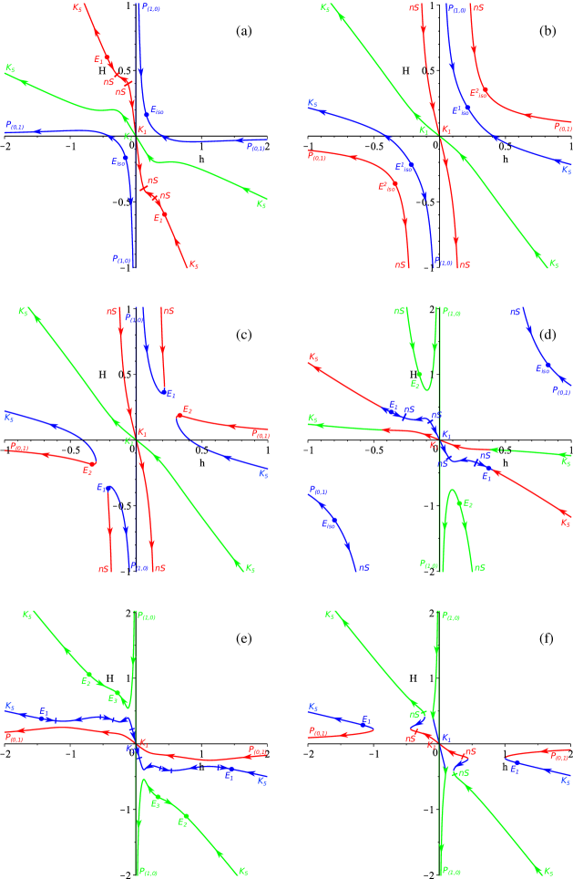
Figure 1: Final compilations of all possible regimes in $D=5$ vacuum cubic Lovelock case, on $H(h)$ evolution curves; different colors correspond to three different branches $H_{1}$, $H_{2}$ and $H_{3}$; panels layout is as follows: $\alpha<0$, $\beta<0$ on (a) panel, $\alpha<0$, $\beta>0$, $\mu<5/8$ on (b) panel, $\alpha<0$, $\beta>0$, $\mu>5/8$ on (c) panel, $\alpha>0$, $\beta<0$ on (d) panel, $\alpha>0$, $\beta>0$, $\mu<\mu_{3}$ on (e) panel, and $\alpha>0$, $\beta>0$, $\mu>\mu_{7}$ on (f) panel (see the text for more details).

We analyze the individual $\dot{H}(h)$, $\dot{h}(h)$, $p_{H}$, $p_{h}$ curves and plot the derived regimes directly on $H(h)$ evolution curves (see Fig. 1). The resulting regimes for $\alpha<0$, $\beta<0$, presented in Fig. 1(a), are: $P_{1,0}\leftrightarrow E_{iso}$ and $P_{0,1}\leftrightarrow E_{iso}$ on blue hyperbola-like $H_{2}$ curve, $K_{5}\leftrightarrow K_{1}$ on green $H_{3}$ curve and $K_{5}\leftrightarrow E_{1}$, $nS\leftrightarrow E_{1}$, $nS\leftrightarrow nS$ and $K_{1}\leftrightarrow nS$ on $H_{1}$. One can see that neither of the regimes have compactification feature – $K_{1}$ from $H_{3}$ has $H<0$, $K_{1}$ from $H_{1}$ has $nS$ as past attractor, $E_{1}$ with $H>0$ is unstable.

The next case to consider is $\alpha<0$, $\beta>0$, $\mu<5/8$, presented in Fig. 1(b). The regimes there are: $P_{0,1}\leftrightarrow E_{iso}^{2}$ and $nS\leftrightarrow E_{iso}^{2}$ on hyperbola-like part of $H_{1}$, $nS\leftrightarrow K_{1}$ on the remaining part of $H_{1}$, $P_{1,0}\leftrightarrow E_{iso}^{1}$ and $K_{5}\leftrightarrow E_{iso}^{1}$ on hyperbola-like $H_{2}$, and $K_{5}\leftrightarrow K_{1}$ on $H_{3}$. For the same reasons as in the previous case, $K_{1}$ cannot be called realistic compactifications, and since there are no other candidates, there are no compactifications in this case either.

Previous case naturally followed by $\alpha<0$, $\beta>0$, $\mu>5/8$, presented in Fig. 1(c). On the boundary value, $\mu=5/8$, the isotropic exponential solutions from Fig. 1(b) coincide so that we have one pair instead of two, but the other regimes are the same so we skipped $\mu=5/8$ from separate consideration. The $\mu>5/8$ case has the regimes: $K_{5}\leftrightarrow K_{1}$ on $H_{3}$ and $nS\leftrightarrow K_{1}$ like in previous case, $E_{1}\leftrightarrow nS$ and $E_{1}\leftrightarrow P_{1,0}$ on one banana-like curve and $E_{2}\leftrightarrow P_{0,1}$ and $E_{2}\leftrightarrow K_{5}$ on another banana-like curve. For the same reasons as in the previous cases, $K_{1}$ cannot give us realistic compactification, and $E_{1}$ and $E_{2}$ are located either in first, so that having $H>0$, $h>0$, or in third ($H<0$, $h<0$) quadrants, so that also cannot serve as realistic compactification either. For $\alpha<0$, similar to the previous $D$ cases (see my18b ), there are no realistic compactification regimes.

We proceed with $\alpha>0$, and the first case to consider is $\beta<0$, presented in Fig. 1(d). There on a hyperbola-like part of $H_{2}$ branch we have $P_{0,1}\leftrightarrow E_{iso}$ and $nS\leftrightarrow E_{iso}$ and $P_{1,0}\leftrightarrow E_{2}$ and $nS\leftrightarrow E_{2}$ on edge-shaped part of $H_{3}$ branch. On the latter, $P_{1,0}\to E_{2}$ is viable compactification regime – $E_{2}$ has $H>0$ and $h<0$ and is stable past asymptote. The remaining regimes include $K_{5}\leftrightarrow K_{1}$ which possesses features of the previous cases and so has not compactifications, and the following combination of regimes along $H_{1}-H_{2}$ physical branch: $K_{5}\to E_{1}\leftarrow nS\to nS\leftarrow K_{1}$. The regimes are given according to fourth quadrant, in the second quadrant they are time-reversed. For the similar reasons as in the previous cases, neither of the regimes along $H_{1}-H_{2}$ physical branch have realistic compactification.

The final case to consider is $\alpha>0$, $\beta>0$. The limiting cases – $\mu<\mu_{3}$ and $\mu>\mu_{7}$ are presented in Fig. 1 – Fig. 1(e) for $\mu<\mu_{3}$ and Fig. 1(f) for $\mu>\mu_{7}$; the fine structure between them is presented in Fig. 2: $\mu<\mu_{3}$ (the same as in Fig. 1(e) but detailed range) on (a) panel, $\mu=\mu_{3}$ on (b) panel, $\mu_{4}>\mu>\mu_{3}$ on (c) panel, $\mu=\mu_{4}$ on (d) panel, $\mu_{1}>\mu>\mu_{4}$ on (e) panel, $\mu=\mu_{1}$ on (f) panel, $\mu_{7}>\mu>\mu_{1}$ on (g) panel, $\mu=\mu_{7}$ on (h) panel and $\mu>\mu_{7}$ (the same as in Fig. 1(f) but detailed range) on (i) panel.

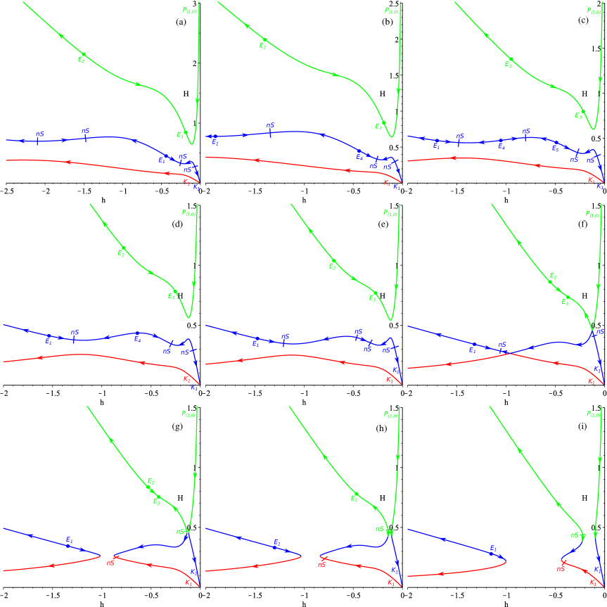
Figure 2: The fine structure of the solutions in the $\alpha>0$, $\beta>0$ $D=5$ vacuum case: $\mu<\mu_{3}$ on (a) panel, $\mu=\mu_{3}$ on (b) panel, $\mu_{4}>\mu>\mu_{3}$ on (c) panel, $\mu=\mu_{4}$ on (d) panel, $\mu_{1}>\mu>\mu_{4}$ on (e) panel, $\mu=\mu_{1}$ on (f) panel, $\mu_{7}>\mu>\mu_{1}$ on (g) panel, $\mu=\mu_{7}$ on (h) panel and $\mu>\mu_{7}$ on (i) panel. Different colors correspond to the different branches (red – to $H_{1}$, blue – to $H_{2}$ and green – to $H_{3}$, in accordance with the designation in Fig. 1) (see the text for more details).

Let us now describe the regimes which appear in these cases. At $\mu<\mu_{3}$ (see Figs. 1(e) and 2(a)) we have $K_{1}\to K_{5}$ along the $H_{1}$ branch (we focus on the second quadrant; the regimes in the fourth quadrant are time-reversal of the described), $K_{1}\leftarrow nS\to nS\leftarrow E_{1}\to nS\leftarrow nS\to K_{5}$ along $H_{2}$ and $P_{1,0}\to E_{3}\leftarrow E_{2}\to K_{5}$ along $H_{3}$. Of these regimes only $P_{1,0}\to E_{3}$ from the $H_{3}$ branch has realistic compactification. For the next several cases the regimes along $H_{1}$ and $H_{3}$ do not change (and so the realistic compactification $P_{1,0}\to E_{3}$ from the $H_{3}$ branch is presented in them as well), the difference is only within $H_{2}$ branch and we describe only these changes. This way, for $\mu=\mu_{3}$ (Fig. 2(b)) along $H_{2}$ we have $K_{1}\leftarrow nS\to nS\leftarrow E_{4}\to nS\leftarrow E_{1}\to K_{5}$ (the outmost $nS$ turned into anisotropic exponential solution), but no new viable compactifications appear; for $\mu_{4}>\mu>\mu_{3}$ (Fig. 2(c)) we have $K_{1}\leftarrow nS\to nS\leftarrow E_{5}\to nS\leftarrow E_{4}\to nS\leftarrow E_{1}\to K_{5}$; for for $\mu=\mu_{4}$ (Fig. 2(d)) we have $K_{1}\leftarrow nS\to nS\leftarrow E_{4}\to nS\leftarrow E_{1}\to K_{5}$; for $\mu_{1}>\mu>\mu_{4}$ (Fig. 2(e)) we have $K_{1}\leftarrow nS\to nS\leftarrow nS\to nS\leftarrow E_{2}\to K_{5}$. One can see that neither of the regimes which appear on $H_{2}$ have realistic compactification. The next case is $\mu=\mu_{1}$, presented in Fig. 2(f) and this is the situation when the physical branches “touch” each other and “reconnecting”, making different “routes”, so that many of the existing regimes terminating and other regimes are formed instead. New regimes could be found on Fig. 2(g), where we plot $\mu_{7}>\mu>\mu_{1}$ case. One can note that the abundance of the exponential solutions and nonstandard singularities is exactly the same as for $\mu_{1}\geqslant\mu>\mu_{4}$ (Figs. 2(e, f)) but the regimes are completely different, since $H(h)$ forming completely different physical branches. So the new regimes for $\mu_{7}>\mu>\mu_{1}$ (Fig. 2(g)) are: $K_{5}\leftarrow E_{1}\to K_{5}$ on the outmost branch, $K_{5}\leftarrow E_{2}\to E_{3}\leftarrow nS\to nS\leftarrow K_{1}$ on the middle branch and $P_{1,0}\to K_{1}$ on the innermost branch. One can see that only the latter gives us realistic compactification – in all other cases $K_{5}$ is future asymptote (or past asymptote but for the regimes in the fourth quadrant, which have $H<0$). Further increase of $\mu$ changing the regimes along middle branch, leaving the outmost and innermost unchanged and so keeping $P_{1,0}\to K_{1}$ as a viable compactification. The change of the regimes along the middle branch is as follows: $K_{5}\leftarrow E_{2}\leftarrow nS\to nS\leftarrow K_{1}$ for $\mu=\mu_{7}$ (see Fig. 2(h)) and $K_{5}\leftarrow nS\to nS\leftarrow K_{1}$ for $\mu>\mu_{7}$ (see Fig. 2(i)); one can see that there are no realistic compactification regimes among those within $H_{2}$.

To conclude, the amount of the viable compactification regimes exactly the same as in $D=4$ case (see my18b ) – in both cases we have $P_{1,0}\to E_{3+D}$ for $\alpha>0$, $\beta<0$ and $P_{1,0}\to E_{3+D}/K_{1}$ for $\alpha>0$, $\beta>0$, $\mu<\mu_{1}$ or $\mu>\mu_{1}$ where $\mu_{1}$ is separating value for $H(h)$. And again, for entire $\alpha>0$ we have realistic compactification regimes.

V General $D\geqslant 6$ case

In this case we use the core (6)–(8) equations – for all $D\geqslant 6$ the structure of the equations of motion is unchanged. Following the procedure, we find the discriminant of (8) with respect to $H$ and then its discriminant with respect to $h$ – it is 16th-order polynomial with respect to $\mu=\beta/\alpha^{2}$ and it has the following roots:

$$\mu_{1}=\displaystyle\frac{D(D+1)}{4(D-1)(D-2)}$$

and $\mu_{2}<\mu_{3}$ – the solutions of certain six-order polynomial with the coefficients made up to $D^{16}$. The expressions for $\mu_{2,3}$ cannot be obtained in terms of elementary functions in the general case but for each $D$ they could be derived, at least numerically. Similar to the previous cases, $\mu_{1}$ separates two different $H(h)$ regimes in $\alpha<0$, $\beta>0$ while $\mu_{2,3}$ – for $\alpha>0$, $\beta>0$, Unlike previous $D=3,4$ cases (see my18b ), where there is only one separation $\mu$ in the $\alpha>0$, $\beta>0$ case, now we have two.

Substituting $\dot{H}=\dot{h}\equiv 0$ and $h\equiv H$ into (6)–(8) gives us single equation which governs isotropic exponential solutions:

$$H^{2}(D+2)(D+3)+\alpha H^{4}D(D+1)(D+2)(D+3)+\beta H^{6}(D-2)(D-1)D(D+1)(D+2)(D+3)=0.$$

Analysis of its nontrivial solution

$$H^{2}=-\displaystyle\frac{\alpha D(D+1)\pm\sqrt{\alpha D^{2}(D+1)^{2}-\beta D(D-2)(D-1)(D+1)}}{\beta D(D-2)(D-1)(D+1)}$$

suggests that there is one isotropic exponential solution for $\beta<0$ (for both signs of $\alpha$) and two for $\alpha<0$, $\beta>0$, $\mu<\mu_{1}$. Let us note that this is the same scheme we had for all previous cases, making it true for all $D$.

The situation with anisotropic exponential solutions is more complicated. Following usual procedure, we obtain equation for $h$ as bi-nine-power polynomial with the discriminant being 24th-order polynomial in $\mu$ with coefficients made up to $D^{130}$. Interesting enough, in the general case there are only two roots of this discriminant which affect the structure of the anisotropic exponential solutions: $\mu_{1}$ – the same as in $H(h)$ and isotropic exponential solutions – and

$$\mu_{4}=-\displaystyle\frac{D^{4}+30G^{3}+189D^{2}-540D+324}{D^{4}-6D^{3}-25D^{2}+102D-72}.$$

So that we can say that in the general $D\geqslant 6$ case there is no “fine structure” of the anisotropic exponential solutions – at least not in the sense we have it for $D=3,4,5$. One can also note that $\mu_{2,3,4}$ have different locations at different $D$: $\mu_{3}>\mu_{4}>\mu_{2}>0$ for $D=6$, $\mu_{4}>\mu_{3}>\mu_{2}>0$ for $D=7$ and $\mu_{4}<0$ for $D\geqslant 8$. So that these three cases have slightly different dynamics and we decided to describe them separately. We fully describe $D=6$ and then describe the changes and new regimes which come from $D=7$ and $D\geqslant 8$.

V.1 $D=6$ case

First let us write down the values for $\mu_{i}$ in this case. So $\mu_{1}=21/40=0.525$, $\mu_{2}\approx 0.2151$, $\mu_{3}\approx 0.3382$ and $\mu_{4}=0.3$.

We perform the same procedure as in the previous cases and obtain the resulting regimes on the $H(h)$ curves; we present them in Fig. 3. As always, different colors correspond to different branches: $H_{1}$ is red, $H_{2}$ is blue and $H_{3}$ is green. The panels layout is the following: $\alpha<0$, $\beta<0$ presented on (a) panel, $\alpha<0$, $\beta>0$, $\mu<\mu_{1}$ on (b) panel, $\alpha<0$, $\beta>0$, $\mu>\mu_{2}$ on (c) panel, $\alpha>0$, $\beta<0$ on (d) panel, $\alpha>0$, $\beta>0$, $\mu<\mu_{2}$ on (e) panel, and $\alpha>0$, $\beta>0$, $\mu>\mu_{3}$ on (f) panel. Let us now describe the regimes.

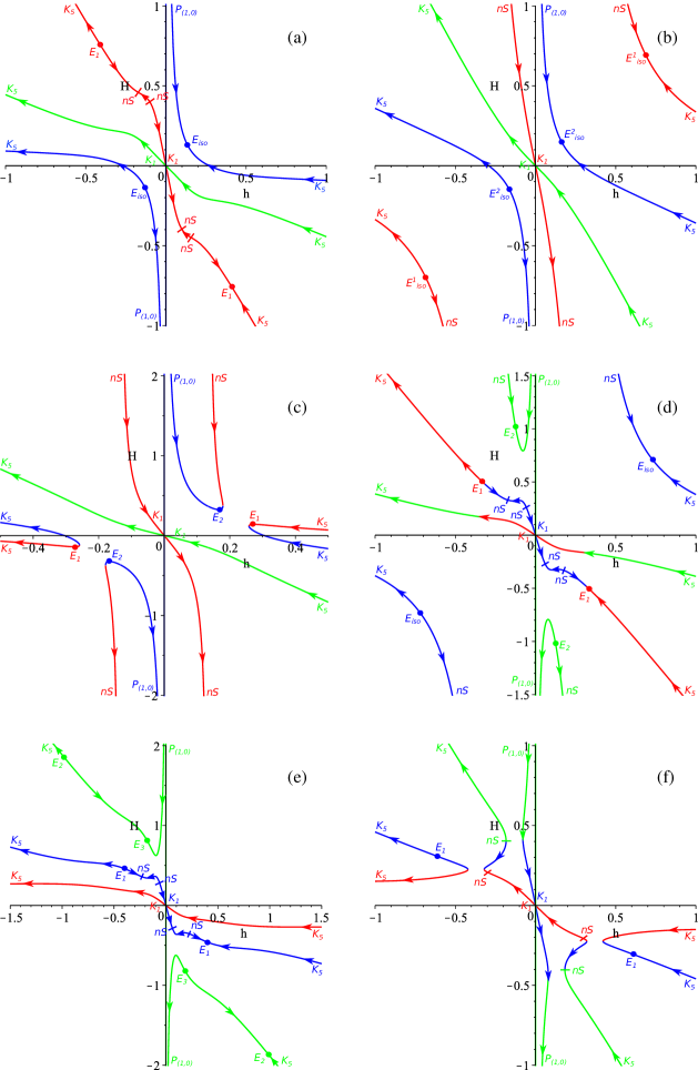
Figure 3: Final compilations of all possible regimes in $D=6$ vacuum cubic Lovelock case, on $H(h)$ evolution curves; different colors correspond to three different branches $H_{1}$, $H_{2}$ and $H_{3}$; panels layout is as follows: $\alpha<0$, $\beta<0$ on (a) panel, $\alpha<0$, $\beta>0$, $\mu<\mu_{1}$ on (b) panel, $\alpha<0$, $\beta>0$, $\mu>\mu_{1}$ on (c) panel, $\alpha>0$, $\beta<0$ on (d) panel, $\alpha>0$, $\beta>0$, $\mu<\mu_{2}$ on (e) panel, and $\alpha>0$, $\beta>0$, $\mu>\mu_{3}$ on (f) panel (see the text for more details).

The first case to consider, $\alpha<0$, $\beta<0$, is presented in Fig. 3(a). There one can see $K_{5}\leftrightarrow E_{iso}$ and $P_{1,0}\leftrightarrow E_{iso}$ on hyperbola-like $H_{2}$ branch, $K_{5}\leftrightarrow K_{1}$ on $H_{3}$ and a number of regimes along $H_{1}$ (according to the second quadrant; in fourth quadrant they are time-reversed): $K_{5}\leftarrow E_{1}\to nS\leftarrow nS\to K_{1}$. One can see that neither of the listed regimes have viable compactification: $E_{1}$ is either unstable or has $H<0$, as for $K_{1}$, it is either past attractor or has $H<0$, or has $nS$ as a past attractor.

The next case is $\alpha<0$, $\beta>0$, $\mu<\mu_{1}$ and it is presented in Fig. 3(b). There we have $K_{5}\leftrightarrow E_{iso}^{1}$ and $nS\leftrightarrow E_{iso}^{2}$ on hyperbola-like part of $H_{1}$ branch and $nS\leftrightarrow K_{1}$ on the remaining part, $K_{5}\leftrightarrow E_{iso}^{2}$ and $P_{1,0}\leftrightarrow E_{iso}^{2}$ on $H_{2}$ and $K_{5}\leftrightarrow K_{1}$ on $H_{3}$. Similar to the previous case (and for the similar reasons) there are no realistic compactification schemes in this case as well.

Similarly to previously considered $D$ cases, at $\mu=\mu_{1}$ the isotropic exponential solutions $E_{iso}^{1}$ and $E_{iso}^{2}$ “touch” each other and coincide; the regimes remain the same so we skip this case from consideration.

With further increase of $\mu$ we have the next case – $\alpha<0$, $\beta>0$, $\mu>\mu_{1}$, presented in Fig. 3(c). Again, similar to the previous $D$ cases, isotropic exponential solutions switched into anisotropic ones; hyperbola-like branches, which “touch” each other at $\mu=\mu_{1}$, “detouch” and form new physical “banana-shaped” branches with the exponential solutions are located on them – one at a branch. So on one of them we have $K_{5}\leftrightarrow E_{1}$ with two different $K_{5}$, on another $nS\leftrightarrow E_{2}$ and $P_{1,0}\leftrightarrow E_{2}$; there are also $nS\leftrightarrow K_{1}$ and $K_{1}\leftrightarrow K_{5}$ on $H_{3}$ – the sane as in previous cases. One can see that $E_{1}$ and $E_{2}$ in the third quadrant are unstable while those in the first are stable but have $H>0$ and $h>0$ so they cannot describe realistic compactification. The comments about $K_{1}$ from the previous cases are true here as well, so there are no viable compactification in this case. To conclude, similarly to the previous $D$ cases, $\alpha<0$ domain does not have realistic compactification regimes.

Now let us turn to $\alpha>0$. The first of these cases is $\beta<0$, presented in Fig. 3(d). The regimes for this case are: $K_{5}\leftrightarrow E_{iso}$ and $nS\leftrightarrow E_{iso}$ on hyperbola-like $H_{2}$ part, $P_{1,0}\leftrightarrow E_{2}$ and $nS\leftrightarrow E_{2}$ on the edge-shaped $H_{3}$ part; among them $P_{1,0}\to E_{2}$ is a realistic compactification regime. Other regimes include $K_{5}\to K_{1}$ on one and $K_{5}\leftarrow E_{1}\to nS\leftarrow nS\to K_{1}$ on another physical branch, listed according to the second quadrant. Let us note that the listed regimes along the second branch are exactly the same as in the described above $\alpha<0$, $\beta<0$ case (see Fig. 3(a)). So that in this case we have one viable compactification regime – $P_{1,0}\to E_{2}$.

What remains is the description of the cases for $\alpha>0$, $\beta>0$. The first of the $\alpha>0$, $\beta>0$ cases, $\mu<\mu_{2}$, is presented in Fig. 3(e), the following cases – in Fig. 4 and the last case, $\mu>\mu_{3}$, in Fig. 3(f). In this regard, we called the subcases in Fig. 4 as a “fine-structure” of the $\alpha>0$, $\beta>0$ case, but it is not in the same sense as previous $D$ cases. In the previous $D$ cases we have fine-structure with respect to the rapid change in the number of exponential solutions – within a small $\mu$ region, the exponential solutions appear, disappear, merge, turn in $nS$ – they have rich and rapid-changing dynamics. In this case we does not have all of this, but we have change of the physical branches. So the manner is the same and so we keep the name “fine-structure”. The subcases within it are presented in Fig. 4 and the panel layout is as follows: $\mu=\mu_{2}$ is on (a) panel, $\mu_{4}>\mu>\mu_{2}$ is on (b) panel, $\mu=\mu_{4}$ is on (c) panel, $\mu_{3}>\mu>\mu_{4}$ is on (d) panel and $\mu=\mu_{3}$ is on (e) panel.

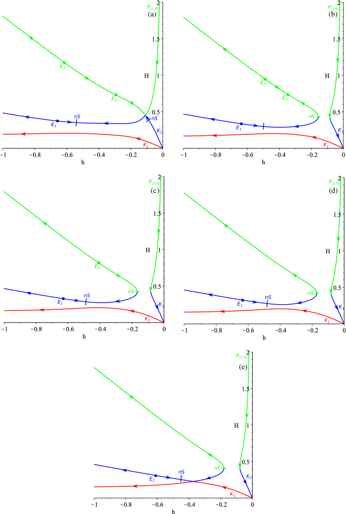
Figure 4: The fine structure of the solutions in the $\alpha>0$, $\beta>0$ $D=6$ vacuum case: $\mu=\mu_{2}$ on (a) panel, $\mu_{4}>\mu>\mu_{2}$ on (b) panel, $\mu=\mu_{4}$ on (c) panel, $\mu_{3}>\mu>\mu_{4}$ on (d) panel and $\mu=\mu_{3}$ on (e) panel. Different colors correspond to different branches: $H_{1}$ is red, $H_{2}$ is blue and $H_{3}$ is green, in accordance with Fig. 3 (see the text for more details).

Let us start with $\mu<\mu_{2}$ case, presented in Fig. 3(e). The regimes for this case are (we list them according to the second quadrant): $K_{1}\to K_{5}$ on $H_{1}$, $K_{5}\leftarrow E_{1}\to nS\leftarrow nS\to K_{1}$ on $H_{2}$ and $K_{5}\leftarrow E_{2}\to E_{3}\leftarrow P_{1,0}$. Of all the regimes, only $P_{1,0}\to E_{3}$ have realistic compactification. The next case is $\mu=\mu_{2}$, presented in Fig. 4(a). Here one can immediately see the difference between $D=4,5$ and the general $D\geqslant 6$ cases – one can see that there are two touching points for the branches and in $D=4,5$ they touch and decouple at the same $\mu$ (see e.g. Fig. 2(f)). But in the general $D\geqslant 6$ they touch and decouple at two different $\mu$ – one at a time – and this is the reason for “fine-structured” consideration of the $\alpha>0$, $\beta>0$ case. The regimes in this case are the same as for $\mu<\mu_{2}$. Once $\mu$ is increased to $\mu_{4}>\mu>\mu_{2}$, the regimes changes and are presented in Fig. 4(b). The regimes are: $P_{1,0}\to K_{1}$, $K_{1}\to K_{5}$ and $K_{5}\leftarrow E_{2}\to E_{3}\leftarrow nS\to nS\leftarrow E_{1}\to K_{5}$. Of them, only $P_{1,0}\to K_{1}$ has realistic compactification. The next case is $\mu=\mu_{4}$, presented in Fig. 4(c), and at this point the number of the exponential solution changes. So that instead of a pair of anisotropic exponential solutions $E_{2}$ and $E_{3}$ on $H_{3}$, we have singe meta-stable ($\sum H=0$ – constant-volume solution, see CST2 ) $E_{2}$. The $P_{1,0}\to K_{1}$ and $K_{1}\to K_{5}$ regimes remain unchanged and the regimes list with anisotropic exponential solution is: $K_{5}\leftarrow E_{2}\leftarrow nS\to nS\leftarrow E_{1}\to K_{5}$. The same as in previous case, only $P_{1,0}\to K_{1}$ has realistic compactification. With further increase of $\mu$, for $\mu_{3}>\mu>\mu_{4}$, presented in Fig. 4(d), even $E_{2}$ disappears, leaving $K_{5}\leftarrow nS\to nS\leftarrow E_{1}\to K_{5}$ in addition to $P_{1,0}\to K_{1}$ and $K_{1}\to K_{5}$ to the list of regimes; of them only $P_{1,0}\to K_{1}$ has realistic compactification. With further increase to $\mu=\mu_{3}$, the second “touch” happening – see Fig. 4(e). And finally the situation for $\mu>\mu_{3}$ is presented in Fig. 3(f). The regimes there are: $P_{1,0}\to K_{1}$, $K_{5}\leftarrow E_{1}\to K_{5}$ (two different $K_{5}$) and $K_{5}\leftarrow nS\to nS\leftarrow K_{1}$. One can see that of them only $P_{1,0}\to K_{1}$ has viable compactification.

This finalize our study of $D=6$ vacuum case. We see that the dynamics and its features are different from the previous cases, but the regimes with realistic compactification and their abundance is the same: all of the regimes require $\alpha>0$ and there are two distinct regimes – $P_{1,0}\to E_{3+6}$ for $\mu<\mu_{2}$ (including $\beta<0$) and $P_{1,0}\to K_{1}$ for $\mu>\mu_{2}$.

V.2 $D=7$ case

The values for $\mu_{i}$ for $D=7$ are: $\mu_{1}=7/15\approx 0.4667$, $\mu_{2}\approx 0.2324$, $\mu_{4}\approx 0.4084$ and $\mu_{4}=289/405\approx 0.7136$. One can see that in the previous $D=6$ case we had $\mu_{3}>\mu_{4}>\mu_{2}$ – the disappearance of the exponential solutions along $H_{3}$ branch happened between the decouplings (at $\mu_{2,3}$. Now, in $D=7$ case, we have $\mu_{4}>\mu_{3}>\mu_{2}$ – the disappearance should happen after the second decoupling. So that the regimes up to $\alpha>0$, $\beta>0$, $\mu_{4}>\mu>\mu_{2}$ (Fig. 4(b)) are exactly the same with the difference that now Fig. 4(b) serves as a representative for $\mu_{3}>\mu>\mu_{2}$ range. The remaining cases for $D=7$ are shown in Fig. 5. As always, different colors correspond to three different branches: $H_{1}$ is red, $H_{2}$ is blue and $H_{3}$ is green, and the panels layout is the following: $\mu_{3}>\mu>\mu_{2}$ in Fig. 5(a), $\mu=\mu_{3}$ in Fig. 5(b), $\mu_{4}>\mu>\mu_{3}$ in Fig. 5(c) and $\mu=\mu_{4}$ in Fig. 5(d); for $\mu>\mu_{4}$ the situation and the regimes are the same as in $\mu>\mu_{3}$ for $D=6$ and so are presented in Fig. 3(f).

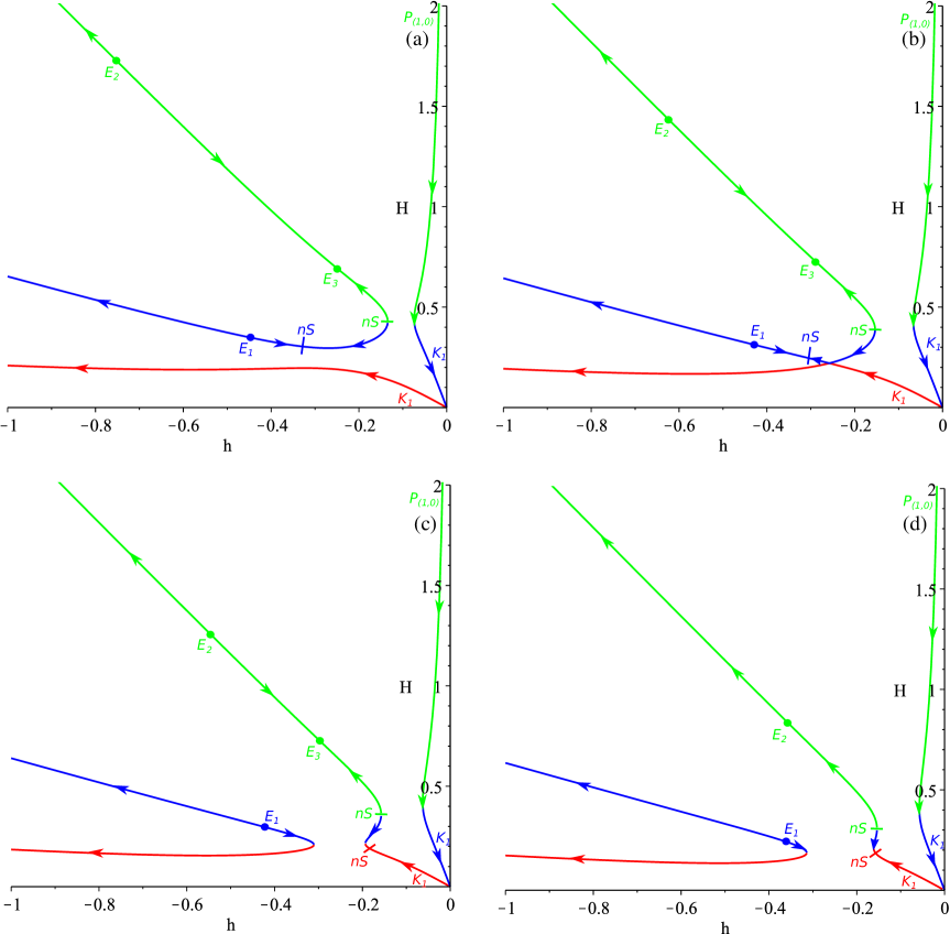
Figure 5: Additional regimes which emerge in $D=7$ vacuum cubic Lovelock case, on $H(h)$ evolution curves; different colors correspond to three different branches $H_{1}$, $H_{2}$ and $H_{3}$; panels layout is as follows: $\mu_{3}>\mu>\mu_{2}$ on (a) panel, $\mu=\mu_{3}$ on (b) panel, $\mu_{4}>\mu>\mu_{3}$ on (c) panel and $\mu=\mu_{4}$ on (d) panel (see the text for more details).

Let us have a closer look on new regimes in this case. The first case, $\mu_{3}>\mu>\mu_{2}$, is presented in Fig. 5(a) and is exactly the same as $\mu_{4}>\mu>\mu_{2}$ from $D=6$, presented in Fig. 4(b) (one can compare and verify that the regimes are the same). Then, the regime with realistic compactification is also the same – it is $P_{1,0}\to K_{1}$. The next case is $\mu=\mu_{3}$, presented in Fig. 5(b) – the second “detouch” – and the regimes are the same. With further increase of $\mu$ to the $\mu_{4}>\mu>\mu_{3}$ range, the situation is presented in Fig. 5(c) and the regimes are: $P_{1,0}\to K_{1}$, $K_{5}\leftarrow E_{1}\to K_{5}$ (with two different $K_{5}$) and $K_{5}\leftarrow E_{2}\to E_{3}\leftarrow nS\to nS\leftarrow K_{1}$. One can see that the regimes along the last mentioned branch are the same as they are in the appropriate $\mu$ range for $D=6$. The realistic compactification in this case is only $P_{1,0}\to K_{1}$. The next case is $\mu=\mu_{4}$, presented in Fig. 5(d), and the changes are the same as they are in $D=6$ – a pair of anisotropic exponential solutions $E_{2}$ and $E_{3}$ collapsed to a single $E_{2}$ with $\sum H=0$; the regimes are $K_{5}\leftarrow E_{2}\leftarrow nS\to nS\leftarrow K_{1}$ and the only realistic compactification regime is $P_{1,0}\to K_{1}$. Finally, for $\mu>\mu_{4}$ $E_{2}$ also disappears and the situation and the regimes are identical to those in $\mu>\mu_{3}$ $D=6$ case, presented in Fig. 3(f).

This concludes our study of $D=7$ vacuum case. We see that the regimes demonstrate difference from $D=6$ case, but the realistic compactifications and their abundances remain the same: all regimes require $\alpha>0$ and there are two of them – $P_{1,0}\to E_{3+7}$ for $\mu<\mu_{2}$ (including $\beta<0$) and $P_{1,0}\to K_{1}$ for $\mu>\mu_{2}$.

V.3 General $D\geqslant 8$ case

As we have learned previously, $\mu_{4}$ is the value for $\mu$ where the change of the number of anisotropic exponential solutions occurs. In all previous cases $D=3\div 7$ this value is positive, so that this change is happening in $\alpha>0$, $\beta>0$. But starting $D\geqslant 8$ it is negative, so that the change happening at $\alpha>0$, $\beta<0$. As a result, the regimes for $\alpha<0$ are exactly the same as in $D=6,7$ (see Figs. 3(a)–(c)), and there are no realistic compactifications. New regimes appear starting $\alpha>0$, $\beta<0$ are they are presented in Fig. 6. As usual, different colors correspond to three different branches: $H_{1}$ is red, $H_{2}$ is blue and $H_{3}$ is green, and the panels layout is the following: $\alpha>0$, $\beta<0$, $\mu<\mu_{4}$ is in Fig. 6(a), $\alpha>0$, $\beta<0$, $\mu=\mu_{4}$ is in Fig. 6(b), $\alpha>0$, $\beta<0$, $\mu>\mu_{4}$ is in Fig. 6(c), $\alpha>0$, $\beta>0$, $\mu<\mu_{2}$ is in Fig. 6(d), $\alpha>0$, $\beta>0$, $\mu_{3}>\mu>\mu_{2}$ is in Fig. 6(e) and $\alpha>0$, $\beta>0$, $\mu>\mu_{3}$ is in Fig. 6(f). We skipped cases with exact $\mu=\mu_{2,3}$ as the situation with exact value was described above. Let us have a closer look on individual panels.

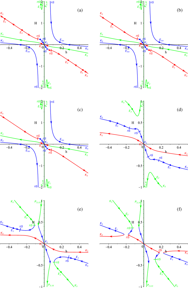
Figure 6: Additional regimes which emerge in $D\geqslant 8$ vacuum cubic Lovelock case, on $H(h)$ evolution curves; different colors correspond to three different branches $H_{1}$, $H_{2}$ and $H_{3}$; panels layout is as follows: $\alpha>0$, $\beta<0$, $\mu<\mu_{4}$ on (a) panel, $\alpha>0$, $\beta<0$, $\mu=\mu_{4}$ on (b) panel, $\alpha>0$, $\beta<0$, $\mu>\mu_{4}$ on (c) panel, $\alpha>0$, $\beta>0$, $\mu<\mu_{2}$ on (d) panel, $\alpha>0$, $\beta>0$, $\mu_{3}>\mu>\mu_{2}$ on (e) panel and $\alpha>0$, $\beta>0$, $\mu>\mu_{3}$ on (f) panel (see the text for more details).

In Fig. 6(a) we have presented $\alpha>0$, $\beta<0$, $\mu<\mu_{4}$ case. One can see that the behavior along hyperbola-like $H_{2}$, edge-shaped part of $H_{3}$ and $H_{1}-H_{3}$ physical branch is the same as in $D=6$ case (compare with Fig. 3(d)), the changes are introduced to $H_{1}-H_{2}$ physical branch. One of the changes regards the number of the anisotropic exponential solutions and another – the time direction of the evolution. One can see that ever since this branch (or its predecessor) appear in $D=4$ (see my18b ) and in following cases $D=5$ (see Fig. 1(d)) and $D=6,7$ (see Fig. 3(d)), $K_{5}$ always was future attractor – the regime was $E_{1}\to K_{5}$. But in $D\geqslant 8$ it is reversed – $K_{5}$ now is past attractor and can serve as a cosmological singularity, making $K_{5}\to E_{1}$ successful compactification. Apart from it, another realistic compactification regime is $P_{1,0}\to E_{2}$ from edge-shaped part of $H_{3}$ branch. The other regimes along the physical branch under consideration include $E_{2}\to E_{1}$, $E_{2}\to nS$, $nS\to nS$ and $K_{1}\to nS$. To conclude, this is the first time in vacuum cubic Lovelock model when we see $K_{5}$ as an origin of viable compactification scheme. The next case is $\alpha>0$, $\beta<0$, $\mu=\mu_{4}$ and it is presented in Fig. 6(b). Similar to the previously considered cases, at $\mu=\mu_{2}$ we have reduction of the anisotropic solutions – $E_{1}$ and $E_{2}$ merge into a single constant volume $E_{1}$ solution; the $K_{5}\to E_{1}$ regime remains, as well as $P_{1,0}\to E_{2}$. With further growth of $\mu$, to $\mu>\mu_{4}$, the situation is presented in Fig. 6(c). One can see that $E_{1}$ disappeared and so we have $K_{5}\to nS$ instead and only $P_{1,0}\to E_{1}$ remains as a realistic compactification regime. So that, for $D\geqslant 8$ at $\alpha>0$, $\beta<0$, $\mu\leqslant\mu_{4}$ we have new realistic compactification regime – $K_{5}\to E_{1}$.

The change of the time direction of one of the branches, described just above, affect $\alpha>0$, $\beta>0$ as well – $K_{5}$ on $H_{3}$ branch, which is future asymptote in $D=4$ (see my18b ), $D=5$ (see Figs. 1(e, f)), $D=6$ (see Figs. 3(e, f)) and $D=7$ (see Figs. 5), now in $D\geqslant 8$ it is a past asymptote, in analogue with $\alpha>0$, $\beta<0$ case described above. So that, similar to the previous case, we have $K_{5}\to E_{2}$ realistic compactification, and it is present for all $\mu>0$ (see Figs. 6(d)–(f)). Another realistic compactification regime is $P_{1,0}\to E_{2}$ for $\mu<\mu_{2}$ (see Fig. 6(d)) and $P_{1,0}\to K_{1}$ for $\mu>\mu_{2}$ (see Figs. 6(e), (f)). The details and other regimes (without compactifications) are quite similar to the analogues in previous case so we skip their consideration.

To conclude, general $D\geqslant 8$ bring us new realistic compactification regime – $K_{5}\to E_{3+D}$ – the only regime with realistic compactification which originates from $K_{5}$. The regime appear for $\alpha>0$, $\beta<0$, $\mu\leqslant\mu_{4}$ and the entire $\alpha>0$, $\beta>0$.

VI Discussions

In the current paper we have analyzed the cosmological dynamics of the cubic Lovelock gravity, with Einstein-Hilbert and Gauss-Bonnet terms present as well. We have chosen a setup with a topology being a product of two isotropic subspaces – three-dimensional, representing our Universe, and $D$-dimensional, representing extra dimensions. Both subspaces are flat, which simplifies our equations of motion and makes it possible to analyze them analytically. Current paper is a direct continuation of my18b where we considered low-$D$ ($D=3,4$) cases and in current paper we extend the analysis on the remaining high-$D$ cases. In a sense, it is also a logical continuation of my16a ; my16b ; my17a ; my18a , where we considered the same problem but in EGB gravity – vacuum case in my16a ; my18a and $\Lambda$-term case in my16b ; my17a ; my18a . In my18a we reviewed all the results for EGB from my16a ; my16b ; my17a and changed the visualization of the regimes – in the original papers my16a ; my16b ; my17a we use tables to list of all the regimes, and this way sometimes is not easy to read. On the contrary, in my18a we put all the regimes on $H(h)$ curves and added arrows to demonstrate $t\to\infty$ directed evolution. In the current paper we decided to keep visualization from my18a .

First of all, let us summarize the results, as they are scattered over mini-conclusions in each particular sections here and in my18b . The fist case is $D=3$, presented in my18b and it has interesting feature – since the equations of motion are cubic in both $H$ and $h$, there could be up to three branches of the solutions. On the other hand, it is the lowest possible dimension for cubic Lovelock gravity, so there are no Kasner solutions (see PT ). Then the only possibility is what we call “generalized Taub” solution – the situation when the expansion in each direction is characterized by Kasner exponent $p_{i}=-H_{i}^{2}/\dot{H}_{i}$ equal to either 1 or 0; so that for our topology it is either $P_{1,0}$ ($p_{H}=1,p_{h}=0$ – expansion of the three-dimensional subspace and “static” extra dimensions) or $P_{0,1}$ ($p_{H}=0,p_{h}=1$ – expansion of the extra-dimensional subspace and “static” three dimensions). Then the remaining branches – which cannot be connected to either $P_{1,0}$ or $P_{0,1}$, form closed evolution curves for ($\alpha<0,\beta<0$) and ($\alpha>0,\beta>0$); for ($\alpha<0,\beta>0$) and ($\alpha>0,\beta<0$) they encounter nonstandard singularities (see my18b for details). The realistic compactification regimes are $P_{1,0}/P_{0,1}\to E_{3+3}$ for ($\alpha>0,\beta<0$) and $P_{1,0}/P_{0,1}\to K_{1}$ for ($\alpha>0,\beta>0$); let us note that both of the regimes exist only for $\alpha>0$.

The $D=4$ case has one cubic Lovelock Kasner solution $K_{5}$ but it is still not enough for all branches, so we still nonstandard singularities at ($\alpha<0,\beta>0$) and ($\alpha>0,\beta<0$) while for ($\alpha<0,\beta<0$) and ($\alpha>0,\beta>0$) the evolution curves have complicated shapes. In $D=4$ we still have $P_{1,0}$ regime, but not $P_{0,1}$, and some of the nonstandard singularities have power-law behavior and so designated as $nS/P$. Unlike $D=3$, where the regimes within the fine structure existed on an isolated $H(h)$ curve, in $D=4$ they are located on one of the physical branches connected with $K_{1}$ (see my18b for details). The realistic compactification regimes are $P_{1,0}\to E_{3+4}$ for $\alpha>0$, $\mu<\mu_{1}$ (including entire $\beta<0$) and $P_{1,0}\to K_{1}$, for $\alpha>0$, $\mu>\mu_{1}$ – exactly the same as in $D=3$ case, and again both of the regimes exist only for $\alpha>0$.

In $D=5$ (see Figs. 1 and 2) we have two different $K_{5}$ and a “return” of $P_{0,1}$, and the general evolution curves and the regimes resemble previous cases; the same is true for the realistic compactification regimes – the same $P_{1,0}\to E_{3+5}$ for $\alpha>0$, $\mu<\mu_{1}$ (including entire $\beta<0$) and $P_{1,0}\to K_{1}$, for $\alpha>0$, $\mu>\mu_{1}$. So that, we can conclude that in $D=3,4,5$ the dynamics, with the exception of some features, is generally the same, so as the realistic compactification regimes.

Formally the equations of motion keep the functional form in all $D\geqslant 6$ cases (meaning that no new terms appear, how it was in the lower dimensions), but our analysis suggests that the details of the dynamics – similar to the differences between $D=3,4,5$ – are different in $D=6,7$ and $D\geqslant 8$ cases, so that we considered them separately. With a minor details, the dynamics of $D=6$ (see Fig. 3) and $D=7$ (see Fig. 5) do not differ much from the previous cases, and the realistic compactification regimes are the same. The only difference is absence of the “fine-structure” of anisotropic exponential solutions, but instead we received the “fine-structure” of the $H(h)$ curves. On the other hand, general $D\geqslant 8$ case brought us a whole new regime with realistic compactification – $K_{5}\to E_{3+D}$ – a regime which originates from “normal” Kasner regime, instead of $P_{1,0}$. This regime exist in two domains: $\alpha>0$, $\beta<0$, $\mu\leqslant\mu_{4}$ and entire $\alpha>0$, $\beta>0$. The regimes $P_{1,0}\to E_{1}$ and $P_{1,0}\to K_{1}$ are also present in the general $D\geqslant 8$ case.

To conclude the situation with the realistic compactifications, for all $D\geqslant 3$ there are $P_{1,0}\to E_{3+D}$ regime for $\alpha>0$, $\mu<\mu_{1}$ (including entire $\beta<0$) and $P_{1,0}\to K_{1}$ regime for $\alpha>0$, $\mu>\mu_{1}$. For $D\geqslant 8$ there is additional regime $K_{5}\to E_{3+D}$ which exists in two domains: $\alpha>0$, $\beta<0$, $\mu\leqslant\mu_{4}$ and entire $\alpha>0$, $\beta>0$. Let us note that for $D\geqslant 8$ and $\alpha>0$, $\beta<0$, $\mu<\mu_{4}$ there are two realistic compactification regimes which exist at the same time and have two different anisotropic exponential solutions as a future asymptotes – $K_{5}\to E_{1}$ along $H_{2}$ branch and $P_{1,0}\to E_{3}$ on edge-shaped part of $H_{3}$ branch (see Fig. 6(a)). For $D\geqslant 8$ and $\alpha>0$, $\beta>0$, $\mu<\mu_{2}$ there are two realistic compactification regimes but they lead to the same anisotropic exponential solution – $K_{5}\to E_{2}$ and $P_{1,0}\to E_{2}$, both on the same $H_{3}$ branch (see Fig. 6(d)).

The above-mentioned “generalized Taub” solution deserves additional comments. Formally it fits the description of the “generalized Milne” solution – the second branch of the power-law solutions in Lovelock gravity (see prd09 for details), but only formally – it fits only because it is degenerative. As we demonstrated in PT , strict “generalized Milne” cannot exist in pure highest-order Lovelock gravity, as it leads to degeneracy in the equations of motion. But if additional (lower-order) Lovelock contributions are involved, it this branch of solutions could be restored, but it was never demonstrated before. So that on the particular example of $[3+D]$ spatial splitting we demonstrated this possibility. Still, a little is known about this regime and it deserves additional investigation in the separate papers.

When we consider this “generalized Taub” solution as a past asymptote – and this is the case for all possible realistic compactification models in $D=3\div 7$ – it feels unnatural. Indeed – the $P_{1,0}$ regime imply $H\to\infty$ and $h\to 0$ as $t\to 0$ (by “0” we mean here initial cosmological singularity), so that we initially have “burst”-like expansion of three-dimensional subspace while the extra-dimensional subspace is almost static. In addition to the feeling of unnaturalness, it is a question if this regime could be reached from totally anisotropic space, in a manner it was done in PT2017 for Kasner regimes in EGB case. So that it gives additional reason to deeply investigate this regime and we are going to do it in the nearest time.

Similar to the results of my18b , the results of this paper suggest that the variety and abundance of the regimes is closer to $\Lambda$-term EGB, rather then to the vacuum EGB models. The reasons for that are not exactly clear, but we suspect that number of the free parameters plays a role here. Indeed, for vacuum EGB model there is only one parameter – $\alpha$, Gauss-Bonnet coupling, while for $\Lambda$-term EGB and vacuum cubic Lovelock there are two – $\alpha$ and $\Lambda$ for the former and $\alpha$ and $\beta$ (cubic Lovelock coupling) for the latter. So that we expect that the dynamics of the $\Lambda$-term cubic Lovelock gravity to be even more interesting and we are going to consider this case shortly.

VII Conclusions

This concludes our study of the cosmological models in vacuum cubic Lovelock gravity. We have found that in all $D\geqslant 3$ there are compactification regimes of two kinds, the first of them originate from “generalized Taub” solution; for the future asymptote we have either Kasner regime or anisotropic exponential solution. In $D\geqslant 8$ there appears another compactification scheme which originates from high-energy Kasner regime and has anisotropic exponential solution as future asymptote. So that for $D\geqslant 8$ and some parameter the two of them coexist on different branches - the situation we never had in EGB gravity.

In addition to the regimes with successful compactification, we described and plotted on $H(h)$ curves all possible transitions for all initial conditions and all structurally different cases. The variety and abundance of the regimes exceed even $\Lambda$-term EGB case, featuring transition between two anisotropic exponential solutions and transition between two different “generalized Taub” solutions.

There are two interesting observations which require additional investigation, as both are quite unexpected. First of them is that all of the realistic compactification regimes have $\alpha>0$ requirement. This is unexpected, as in both vacuum and $\Lambda$-term EGB cases we have viable compactifications for both signs of $\alpha$. We can note that for the $\Lambda$-term case the joint analysis of our cosmological bounds and those coming from AdS/CFT and other considerations allows us to conclude $\alpha>0$ (see my16b ; my18a ), but for that we involved external (to our analysis) results. On the contrary, in the current case without any external bounds we already have realistic compactification only for $\alpha>0$.

The second observation is that there is no $K_{5}\to K_{1}$ transition with realistic compactification. In EGB vacuum case my16a ; my18a we have the transitions of this kind, so we expected that in the higher-order Lovelock gravity they would also appear, but our investigation reveals that they do not. There is $K_{5}\to K_{1}$ transition, but with contracting three and expanding extra dimensions, so it formally exist, but with no realistic compactification. As both of these observations are unexpected and are in disagreement with what we have learned from study of EGB case, this is a good direction for further improvement of our understanding of Lovelock gravity.

In fact, the cubic (and higher-order) Lovelock gravities are studied much less then the Gauss-Bonnet gravity (which is quadratic Lovelock gravity) – apart from the above-mentioned papers, we studied some properties of the power-law prd09 and exponential CST2 solutions and studied the stability of the latter my15 . Additionally, some properties of models with spatial curvature are studied in CGT18 . Our results suggest that there are some interesting features making the dynamics of the cubic Lovelock gravity different from EGB case, which increase the significance of the results and stimulate further investigation of cubic and higher-order Lovelock cosmologies.

References

- (1) G. Nordström, Phys. Z. 15, 504 (1914).
- (2) G. Nordström, Ann. Phys. (Berlin) 347, 533 (1913).
- (3) A. Einstein, Ann. Phys. (Berlin) 354, 769 (1916).
- (4) T. Kaluza, Sit. Preuss. Akad. Wiss. K1, 966 (1921).
- (5) O. Klein, Z. Phys. 37, 895 (1926).
- (6) O. Klein, Nature (London) 118, 516 (1926).
- (7) J. Scherk and J.H. Schwarz, Nucl. Phys. B81, 118 (1974).
- (8) M.A. Virasoro, Phys. Rev. 177, 2309 (1969).
- (9) J.A. Shapiro, Phys. Lett. 33B, 361 (1970).
- (10) P. Candelas, G.T. Horowitz, A. Strominger and E. Witten, Nucl. Phys. B258, 46 (1985).
- (11) D.J. Gross, J.A. Harvey, E. Martinec and R. Rohm, Phys. Rev. Lett. 54, 502 (1985).
- (12) B. Zwiebach, Phys. Lett. 156B, 315 (1985).
- (13) C. Lanczos, Z. Phys. 73, 147 (1932).
- (14) C. Lanczos, Ann. Math. 39, 842 (1938).
- (15) B. Zumino, Phys. Rep. 137, 109 (1986).
- (16) D. Lovelock, J. Math. Phys. (N.Y.) 12, 498 (1971).
- (17) F. Mller-Hoissen, Phys. Lett. 163B, 106 (1985).
- (18) N. Deruelle and L. Fariña-Busto, Phys. Rev. D 41, 3696 (1990).
- (19) F. Mller-Hoissen, Class. Quant. Grav. 3, 665 (1986).
- (20) S.A. Pavluchenko, Phys. Rev. D 80, 107501 (2009).
- (21) J. Demaret, H. Caprasse, A. Moussiaux, P. Tombal, and D. Papadopoulos, Phys. Rev. D 41, 1163 (1990).
- (22) G. A. Mena Marugán, Phys. Rev. D 46, 4340 (1992).
- (23) E. Elizalde, A.N. Makarenko, V.V. Obukhov, K.E. Osetrin, and A.E. Filippov, Phys. Lett. B644, 1 (2007).
- (24) K.I. Maeda and N. Ohta, Phys. Rev. D 71, 063520 (2005).
- (25) K.I. Maeda and N. Ohta, JHEP 1406, 095 (2014).
- (26) J.T. Wheeler, Nucl. Phys. B268, 737 (1986).
- (27) T. Torii and H. Maeda, Phys. Rev. D 71, 124002 (2005).
- (28) T. Torii and H. Maeda, Phys. Rev. D 72, 064007 (2005).
- (29) Sh. Nojiri and S. D. Odintsov, Phys. Lett. B521, 87 (2001); ibid B542, 301 (2002).
- (30) Sh. Nojiri, S. D. Odintsov and S. Ogushi , Int. J. Mod. Phys. A 17, 4809 (2002).
- (31) M. Cvetic, Sh. Nojiri and S. D. Odintsov, Nucl. Phys. B628, 295 (2002).
- (32) R.G. Cai, Phys. Rev. D 65, 084014 (2002).
- (33) D.G. Boulware and S. Deser, Phys. Rev. Lett. 55, 2656 (1985).
- (34) D.L. Wilshire. Phys. Lett. B169, 36 (1986).
- (35) R.G. Cai, Phys. Lett. 582, 237 (2004).
- (36) J. Grain, A. Barrau, and P. Kanti, Phys. Rev. D 72, 104016 (2005).
- (37) R.G. Cai and N. Ohta, Phys. Rev. D 74, 064001 (2006).
- (38) X.O. Camanho and J.D. Edelstein, Class. Quant. Grav. 30, 035009 (2013).
- (39) H. Maeda, Phys. Rev. D 73, 104004 (2006).
- (40) M. Nozawa and H. Maeda, Class. Quant. Grav. 23, 1779 (2006).
- (41) H. Maeda, Class. Quant. Grav. 23, 2155 (2006).
- (42) M.H. Dehghani and N. Farhangkhah, Phys. Rev. D 78, 064015 (2008).
- (43) H. Ishihara, Phys. Lett. B179, 217 (1986).
- (44) N. Deruelle, Nucl. Phys. B327, 253 (1989).
- (45) S.A. Pavluchenko and A.V. Toporensky, Mod. Phys. Lett. A24, 513 (2009).
- (46) S.A. Pavluchenko, Phys. Rev. D 82, 104021 (2010).
- (47) V. Ivashchuk, Int. J. Geom. Meth. Mod. Phys. 07, 797 (2010) arXiv: 0910.3426.
- (48) I.V. Kirnos, A.N. Makarenko, S.A. Pavluchenko, and A.V. Toporensky, General Relativity and Gravitation 42, 2633 (2010).
- (49) S.A. Pavluchenko and A.V. Toporensky, Gravitation and Cosmology 20, 127 (2014); arXiv: 1212.1386.
- (50) I.V. Kirnos, S.A. Pavluchenko, and A.V. Toporensky, Gravitation and Cosmology 16, 274 (2010) arXiv: 1002.4488.
- (51) D. Chirkov, S. Pavluchenko, A. Toporensky, Mod. Phys. Lett. A29, 1450093 (2014); arXiv: 1401.2962.
- (52) D. Chirkov, S. Pavluchenko, A. Toporensky, Gen. Rel. Grav. 46, 1799 (2014); arXiv: 1403.4625.
- (53) D. Chirkov, S. Pavluchenko, A. Toporensky, Gen. Rel. Grav. 47, 137 (2015); arXiv:1501.04360.
- (54) S.A. Pavluchenko, Phys. Rev. D 92, 104017 (2015).
- (55) V. D. Ivashchuk, Eur. Phys. J. C 76, 431 (2016).
- (56) F. Canfora, A. Giacomini and S. A. Pavluchenko, Phys. Rev. D 88, 064044 (2013).
- (57) F. Canfora, A. Giacomini and S. A. Pavluchenko, Gen. Rel. Grav. 46, 1805 (2014).
- (58) F. Canfora, A. Giacomini, S. A. Pavluchenko and A. Toporensky, Gravitation and Cosmology 24, 28 (2018).
- (59) S.A. Pavluchenko, Phys. Rev. D 94, 024046 (2016).
- (60) S.A. Pavluchenko, Particles 1, 4 (2018) [arXiv:1803.01887].
- (61) S.A. Pavluchenko, Phys. Rev. D 94, 084019 (2016)
- (62) S.A. Pavluchenko, Eur. Phys. J. C 77, 503 (2017).
- (63) S.A. Pavluchenko and A.V. Toporensky, Eur. Phys. J. C 78, 373 (2018).
- (64) S.A. Pavluchenko, Phys. Rev. D 67, 103518 (2003).
- (65) S.A. Pavluchenko, Phys. Rev. D 69, 021301 (2004).
- (66) S.A. Pavluchenko, Eur. Phys. J. C accepted (2018) [arXiv:1804.06934].
- (67) E. Kasner, Am. J. Math. 43, 217 (1921).
- (68) A.H. Taub, Ann. Math. 53, 472 (1951).
- (69) F.J. Tipler, Phys. Lett. A64, 8 (1977).
- (70) T. Kitaura and J.T. Wheeler, Nucl. Phys. B355, 250 (1991).
- (71) T. Kitaura and J.T. Wheeler, Phys. Rev. D 48, 667 (1993).
- (72) D. Chirkov, A. Giacomini and A. Toporensky, arXiv:1804.02193.