Answering Hindsight Queries with Lifted Dynamic Junction Trees

Abstract

The lifted dynamic junction tree algorithm (LDJT) efficiently answers filtering and prediction queries for probabilistic relational temporal models by building and then reusing a first-order cluster representation of a knowledge base for multiple queries and time steps. We extend LDJT to (i) solve the smoothing inference problem to answer hindsight queries by introducing an efficient backward pass and (ii) discuss different options to instantiate a first-order cluster representation during a backward pass. Further, our relational forward backward algorithm makes hindsight queries to the very beginning feasible. LDJT answers multiple temporal queries faster than the static lifted junction tree algorithm on an unrolled model, which performs smoothing during message passing.

1 Introduction

Areas like healthcare or logistics and cross-sectional aspects such as IT security involve probabilistic data with relational and temporal aspects and need efficient exact inference algorithms, as indicated by ? (?). These areas involve many objects in relation to each other with changes over time and uncertainties about object existence, attribute value assignments, or relations between objects. More specifically, IT security involves network dependencies (relational) for many components (objects), streams of attacks over time (temporal), and uncertainties due to, for example, missing or incomplete information, caused by faulty sensor data. By performing model counting, probabilistic databases can answer queries for relational temporal models with uncertainties (?; ?). However, each query embeds a process behaviour, resulting in huge queries with possibly redundant information. In contrast to PDBs, we build more expressive and compact models including behaviour (offline) enabling efficient answering of more compact queries (online). For query answering, our approach performs deductive reasoning by computing marginal distributions at discrete time steps. In this paper, we study the problem of exact inference, in form of smoothing, in large temporal probabilistic models.

We introduce parameterised probabilistic dynamic models to represent probabilistic relational temporal behaviour and propose the LDJT to exactly answer multiple filtering and prediction queries for multiple time steps efficiently (?). LDJT combines the advantages of the interface algorithm (?) and the lifted junction tree algorithm (LJT) (?). Specifically, this paper extends LDJT and contributes (i) an inter first-order junction tree (FO jtree) backward pass to perform smoothing for hindsight queries, (ii) different FO jtree instantiation options during a backward pass, and (iii) a relational forward backward algorithm. Our relational forward backward algorithm reinstantiates FO jtrees by leveraging LDJT’s forward pass. Without reinstantiating FO jtrees, the memory consumption of keeping all FO jtrees instantiated renders hindsight queries to the very beginning infeasible.

Even though smoothing is a main inference problem, to the best of our knowledge there is no approach solving smoothing efficiently for relational temporal models. Smoothing can improve the accuracy of hindsight queries by back-propagating newly gained evidence. Additionally, a backward pass is required for problems such as learning.

Lifting exploits symmetries in models to reduce the number of instances to perform inference on. LJT reuses the FO jtree structure to answer multiple queries. LDJT also reuses the FO jtree structure to answer queries for all time steps $t>0$. Additionally, LDJT ensures a minimal exact inter FO jtree information propagation. Thus, LDJT propagates minimal information to connect FO jtrees by message passing also during backward passes and reuses FO jtree structures to perform smoothing.

In the following, we begin by introducing PDMs as a representation for relational temporal probabilistic models and present LDJT, an efficient reasoning algorithm for PDMs. Afterwards, we extend LDJT with an inter FO jtrees backward pass and discuss different options to instantiate an FO jtree during a backward pass. Lastly, we evaluate LDJT against LJT and conclude by looking at extensions.

2 Related Work

We take a look at inference for propositional temporal models, relational static models, and give an overview about research regarding relational temporal models.

For exact inference on propositional temporal models, a naive approach is to unroll the temporal model for a given number of time steps and use any exact inference algorithm for static, i.e., non-temporal, models. In the worst case, once the number of time steps changes, one has to unroll the model and infer again. ? (?) proposes the interface algorithm consisting of a forward and backward pass that uses a temporal d-separation with a minimal set of nodes to apply static inference algorithms to the dynamic model.

First-order probabilistic inference leverages the relational aspect of a static model. For models with known domain size, it exploits symmetries in a model by combining instances to reason with representatives, known as lifting (?). ? (?) introduces parametric factor graphs as relational models and proposes lifted variable elimination (LVE) as an exact inference algorithm on relational models. Further, ? (?), ? (?), and ? (?) extend LVE to its current form. ? (?) introduce the junction tree algorithm. To benefit from the ideas of the junction tree algorithm and LVE, ? (?) present LJT that efficiently performs exact first-order probabilistic inference on relational models given a set of queries.

Inference on relational temporal models mostly consists of approximative approaches. Additionally, to being approximative, these approaches involve unnecessary groundings or are only designed to handle single queries efficiently. ? (?) propose lifted (loopy) belief propagation. From a factor graph, they build a compressed factor graph and apply lifted belief propagation with the idea of the factored frontier algorithm (?), which is an approximate counterpart to the interface algorithm and also provides means for a backward pass. ? (?) introduce CPT-L, a probabilistic model for sequences of relational state descriptions with a partially lifted inference algorithm. ? (?) present an online interface algorithm for dynamic Markov logic networks, similar to the work of ? (?). Both approaches slice DMLNs to run well-studied static MLN (?) inference algorithms on each slice. Two ways of performing online inference using particle filtering are described in (?; ?).

? (?) introduce an exact approach for relational temporal models involving computing probabilities of each possible interface assignment.

To the best of our knowledge, none of the relational temporal approaches perform smoothing efficiently. Besides of LDJT’s benefits of being an exact algorithm answering multiple filter and prediction queries for relation temporal models efficiently, we decided to extend LDJT as it offers the ability to reinstatiate previous time steps and thereby make hindsight queries to the very beginning feasible.

3 Parameterised Probabilistic Models

Based on (?), we shortly present parameterised probabilistic models for relational static models. Afterwards, we extend PMs to the temporal case, resulting in PDMs for relational temporal models, which, in turn, are based on (?).

3.1 Parameterised Probabilistic Models

PMs combine first-order logic with probabilistic models, representing first-order constructs using logical variables as parameters. As an example, we set up a PM for risk analysis with an attack graph (AG). An AG models attacks on targeted components in a network. A binary random variable (randvar) holds if a component is compromised, which provides an attacker with privileges to further compromise a network to reach a final target. We use logvars to represent users with certain privileges. The model is inspired by ? (?), who examine exact probabilistic inference for IT security with AGs.

Definition 1.

Let $\mathbf{L}$ be a set of logvar names, $\Phi$ a set of factor names, and $\mathbf{R}$ a set of randvar names. A parameterised randvar (PRV) $A=P(X^{1},...,X^{n})$ represents a set of randvars behaving identically by combining a randvar $P\in\mathbf{R}$ with $X^{1},...,X^{n}\in\mathbf{L}$. If $n=0$, the PRV is parameterless. The domain of a logvar $L$ is denoted by $\mathcal{D}(L)$. The term $range(A)$ provides possible values of a PRV $A$. Constraint $(\mathbf{X},C_{\mathbf{X}})$ allows to restrict logvars to certain domain values and is a tuple with a sequence of logvars $\mathbf{X}=(X^{1},...,X^{n})$ and a set $C_{\mathbf{X}}\subseteq\times_{i=1}^{n}\mathcal{D}(X^{i})$. The symbol $\top$ denotes that no restrictions apply and may be omitted. The term $lv(Y)$ refers to the logvars in some element $Y$. The term $gr(Y)$ denotes the set of instances of $Y$ with all logvars in $Y$ grounded w.r.t. constraints.

From $\mathbf{R}=\{Server,User\}$ and $\mathbf{L}=\{X,Y\}$ with $\mathcal{D}(X)=\{x_{1},x_{2},x_{3}\}$ and $\mathcal{D}(Y)=\{y_{1},y_{2}\}$, we build the boolean PRVs $Server$ and $User(X)$. With $C=(X,\{x_{1},x_{2}\})$, $gr(User(X)|C)=\{User(x_{1}),\linebreak User(x_{2})\}$. $gr(User(X)|\top)$ also contains $User(x_{3})$.

Figure 1: Parfactor graph for $G^{ex}$

Figure 2: $G_{\rightarrow}^{ex}$ the two-slice temporal parfactor graph for model $G^{ex}$

Definition 2.

We denote a parametric factor (parfactor) $g$ with $\forall\mathbf{X}:\phi(\mathcal{A})\;|C$, $\mathbf{X}\subseteq\mathbf{L}$ being a set of logvars over which the factor generalises, $C$ a constraint on $\mathbf{X}$, and $\mathcal{A}=(A^{1},...,A^{n})$ a sequence of PRVs. We omit $(\forall\mathbf{X}:)$ if $\mathbf{X}=lv(\mathcal{A})$. A function $\phi:\times_{i=1}^{n}range(A^{i})\mapsto\mathbb{R}^{+}$ with name $\phi\in\Phi$ is identical for all grounded instances of $\mathcal{A}$. The complete specification for $\phi$ is a list of all input-output values. A PM $G:=\{g^{i}\}_{i=0}^{n-1}$ is a set of parfactors and semantically represents the full joint probability distribution $P_{G}=\frac{1}{Z}\prod_{f\in gr(G)}\phi(f)$ with $Z$ as normalisation constant.

Adding boolean PRVs $Attack1$, $Attack2$, $Admin(Y)$, $Infects(X,Y)$, $G_{ex}=\{g^{i}\}^{4}_{i=0}$, $g^{0}=\phi^{0}(Attack1,User(X))$, $g^{1}=\phi^{1}(Attack2,Admin(Y))$, $g^{2}=\phi^{2}(User(X),Admin(Y),Infects(X,Y))$, $g^{3}=\phi^{3}(Server,User(X))$, and $g^{4}=\phi^{4}(Server,Admin(Y))$ forms a model. $g^{2}$ has eight, the others four input-output pairs (omitted). Constraints are $\top$, i.e., the $\phi$’s hold for all domain values. E.g., $gr(g^{0})$ contains three factors with identical $\phi$. Figure 1 depicts $G^{ex}$ as a graph with six variable nodes for the PRVs and five factor nodes for $g^{0}$ to $g^{4}$ with edges to the PRVs involved. Additionally, we can observe the state of the server. The remaining PRVs are latent.

The semantics of a model is given by grounding and building a full joint distribution. In general, queries ask for a probability distribution of a randvar using a model’s full joint distribution and given fixed events as evidence.

Definition 3.

Given a PM $G$, a ground PRV $Q$ and grounded PRVs with fixed range values $\mathbf{E}$, the expression $P(Q|\mathbf{E})$ denotes a query w.r.t. $P_{G}$.

3.2 Parameterised Probabilistic Dynamic Models

To define PDMs, we use PMs and the idea of how Bayesian networks give rise to dynamic Bayesian networks. We define PDMs based on the first-order Markov assumption, i.e., a time slice $t$ only depends on the previous time slice $t-1$. Further, the underlining process is stationary, i.e., the model behaviour does not change over time.

Definition 4.

A PDM is a pair of PMs $(G_{0},G_{\rightarrow})$ where $G_{0}$ is a PM representing the first time step and $G_{\rightarrow}$ is a two-slice temporal parameterised model representing $\mathbf{A}_{t-1}$ and $\mathbf{A}_{t}$ where $\mathbf{A}_{\pi}$ a set of PRVs from time slice $\pi$.

Figure 2 shows $G_{\rightarrow}^{ex}$ consisting of $G^{ex}$ for time step $t-1$ and $t$ with inter-slice parfactors for the behaviour over time. In this example, the parfactors $g^{A}$ and $g^{U}$ are the inter-slice parfactors, modelling the temporal behavior.

Definition 5.

Given a PDM $G$, a ground PRV $Q_{t}$ and grounded PRVs with fixed range values $\mathbf{E}_{0:t}$ the expression $P(Q_{t}|\mathbf{E}_{0:t})$ denotes a query w.r.t. $P_{G}$.

The problem of answering a marginal distribution query $P(A^{i}_{\pi}|\mathbf{E}_{0:t})$ w.r.t. the model is called prediction for $\pi>t$, filtering for $\pi=t$, and smoothing for $\pi<t$.

4 Lifted Dynamic Junction Tree Algorithm

We start by introducing LJT, mainly based on (?), to provide means to answer queries for PMs. Afterwards, we present LDJT, based on (?), consisting of FO jtree constructions for a PDM and an efficient filtering and prediction algorithm.

4.1 Lifted Junction Tree Algorithm

LJT provides efficient means to answer queries $P(\mathbf{Q}|\mathbf{E})$, with a set of query terms, given a PM $G$ and evidence $\mathbf{E}$, by performing the following steps: (i) Construct an FO jtree $J$ for $G$. (ii) Enter $\mathbf{E}$ in $J$. (iii) Pass messages. (iv) Compute answer for each query $Q^{i}\in\mathbf{Q}$.

We first define an FO jtree and then go through each step. To define an FO jtree, we first need to define parameterised clusters (parclusters), the nodes of an FO jtree.

Definition 6.

A parcluster $\mathbf{C}$ is defined by $\forall\mathbf{L}:\mathbf{A}|C$. $\mathbf{L}$ is a set of logvars, $\mathbf{A}$ is a set of PRVs with $lv(\mathbf{A})\subseteq\mathbf{L}$, and $C$ a constraint on $\mathbf{L}$. We omit $(\forall\mathbf{L}:)$ if $\mathbf{L}=lv(\mathbf{A})$. A parcluster $\mathbf{C}^{i}$ can have parfactors $\phi(\mathcal{A}^{\phi})|C^{\phi}$ assigned given that (i) $\mathcal{A}^{\phi}\subseteq\mathbf{A}$, (ii) $lv(\mathcal{A}^{\phi})\subseteq\mathbf{L}$, and (iii) $C^{\phi}\subseteq C$ holds. We call the set of assigned parfactors a local model $G^{i}$.
An FO jtree for a PM $G$ is $J=(\mathbf{V},\mathbf{E})$ where $J$ is a cycle-free graph, the nodes $\mathbf{V}$ denote a set of parcluster, and the set $\mathbf{E}$ edges between parclusters. An FO jtree must satisfy the properties: (i) A parcluster $\mathbf{C}^{i}$ is a set of PRVs from $G$. (ii) For each parfactor $\phi(\mathcal{A})|C$ in G, $\mathcal{A}$ must appear in some parcluster $\mathbf{C}^{i}$. (iii) If a PRV from $G$ appears in two parclusters $\mathbf{C}^{i}$ and $\mathbf{C}^{j}$, it must also appear in every parcluster $\mathbf{C}^{k}$ on the path connecting nodes i and j in $J$. The separator $\mathbf{S}^{ij}$ containing shared PRVs of edge $i-j$ is given by $\mathbf{C}^{i}\cap\mathbf{C}^{j}$.

LJT constructs an FO jtree using a first-order decomposition tree, enters evidence in the FO jtree, and passes messages through an inbound and an outbound pass, to distribute local information of the nodes through the FO jtree. To compute a message, LJT eliminates all non-seperator PRVs from the parcluster’s local model and received messages. After message passing, LJT answers queries. For each query, LJT finds a parcluster containing the query term and sums out all non-query terms in its local model and received messages.

Figure 3: FO jtree for $G^{ex}$ (local models in grey)

Figure 3 shows an FO jtree of $G^{ex}$ with the local models of the parclusters and the separators as labels of edges. During the inbound phase of message passing, LJT sends messages from $\mathbf{C}^{1}$ and $\mathbf{C}^{3}$ to $\mathbf{C}^{2}$ and during the outbound phase from $\mathbf{C}^{2}$ to $\mathbf{C}^{1}$ and $\mathbf{C}^{3}$. If we want to know whether $Attack1$ holds, we query for $P(Attack1)$ for which LJT can use parcluster $\mathbf{C}^{1}$. LJT sums out $User(X)$ from $\mathbf{C}^{1}$’s local model $G^{1}$, $\{g^{0}\}$, combined with the received messages, here, one message from $\mathbf{C}^{2}$.

Figure 4: Forward and backward pass of LDJT (local models and in- and out-cluster labeling in grey)

4.2 LDJT: Overview

LDJT efficiently answers queries $P(\mathbf{Q}_{t}|\mathbf{E}_{0:t})$, with a set of query terms $\{\mathbf{Q}_{t}\}_{t=0}^{T}$, given a PDM $G$ and evidence $\{\mathbf{E}_{t}\}_{t=0}^{T}$, by performing the following steps:

(i) Offline construction of two FO jtrees $J_{0}$ and $J_{t}$ with in- and out-clusters from $G$ (ii) For $t=0$, using $J_{0}$ to enter $\mathbf{E}_{0}$, pass messages, answer each query term $Q_{\pi}^{i}\in\mathbf{Q}_{0}$, and preserve the state in message $\alpha_{0}$ (iii) For $t>0$, instantiate $J_{t}$ for the current time step $t$, recover the previous state from message $\alpha_{t-1}$, enter $\mathbf{E}_{t}$ in $J_{t}$, pass messages, answer each query term $Q_{\pi}^{i}\in\mathbf{Q}_{t}$, and preserve the state in message $\alpha_{t}$

We begin with LDJT’s FO jtrees construction, which contain a minimal set of PRVs to m-separate the FO jtrees. M-separation means that information about these PRVs make FO jtrees independent from each other. Afterwards, we present how LDJT connects FO jtrees for reasoning to solve the filtering and prediction problems efficiently.

4.3 LDJT: FO Jtree Construction for PDMs

LDJT constructs FO jtrees for $G_{0}$ and $G_{\rightarrow}$, both with an incoming and outgoing interface. To be able to construct the interfaces in the FO jtrees, LDJT uses the PDM $G$ to identify the interface PRVs $\mathbf{I}_{t}$ for a time slice $t$.

Definition 7.

The forward interface is defined as $\mathbf{I}_{t}=\{A_{t}^{i}\mid\exists\phi(\mathcal{A})|C\in G:A_{t}^{i}\in\mathcal{A}\wedge\exists A_{t+1}^{j}\in\mathcal{A}\}$, i.e., the PRVs which have successors in the next slice.

PRVs $User_{t-1}(X)$ and $Admin_{t-1}(Y)$ from $G_{\rightarrow}^{ex}$, shown in Fig. 2, have successors in the next time slice, making up $\mathbf{I}_{t-1}$. To ensure interface PRVs $\mathbf{I}$ ending up in a single parcluster, LDJT adds a parfactor $g^{I}$ over the interface to the model. Thus, LDJT adds a parfactor $g^{I}_{0}$ over $\mathbf{I}_{0}$ to $G_{0}$, builds an FO jtree $J_{0}$, and labels the parcluster with $g^{I}_{0}$ from $J_{0}$ as in- and out-cluster. For $G_{\rightarrow}$, LDJT removes all non-interface PRVs from time slice $t-1$, adds parfactors $g^{I}_{t-1}$ and $g^{I}_{t}$, constructs $J_{t}$, and labels the parcluster containing $g^{I}_{t-1}$ as in-cluster and the parcluster containing $g^{I}_{t}$ as out-cluster.

The interface PRVs are a minimal required set to m-separate the FO jtrees. LDJT uses these PRVs as separator to connect the out-cluster of $J_{t-1}$ with the in-cluster of $J_{t}$, allowing to reuse the structure of $J_{t}$ for all $t>0$.

4.4 LDJT: Reasoning with PDMs

Since $J_{0}$ and $J_{t}$ are static, LDJT uses LJT as a subroutine by passing on a constructed FO jtree, queries, and evidence for step $t$ to handle evidence entering, message passing, and query answering using the FO jtree. Further, for proceeding to the next time step, LDJT calculates an $\alpha_{t}$ message over the interface PRVs using the out-cluster to preserve the information about the current state. Afterwards, LDJT increases $t$ by one, instantiates $J_{t}$, and adds $\alpha_{t-1}$ to the in-cluster of $J_{t}$. During message passing, $\alpha_{t-1}$ is distributed through $J_{t}$. Thereby, LDJT performs an inter FO jtree forward pass to proceed in time. Additionally, due to the inbound and outbound message passing, LDJT also performs an intra backward pass for the current FO jtree.

Figure 4 depicts the passing on of the current state from time step three to four. To capture the state at $t=3$, LDJT sums out the non-interface PRVs $Server_{3}$ and $Admin_{2}(Y)$ from $\mathbf{C}_{3}^{3}$’s local model and the received messages and saves the result in message $\alpha_{3}$. After increasing $t$ by one, LDJT adds $\alpha_{3}$ to the in-cluster of $J_{4}$, $\mathbf{C}_{4}^{2}$. $\alpha_{3}$ is then distributed by message passing and accounted for during calculating $\alpha_{4}$.

5 Smoothing Extension for LDJT

We introduce an inter FO jtree backward pass and extend LDJT with it to also answer smoothing queries efficiently.

5.1 Inter FO Jtree Backward Pass

Using the forward pass, each instantiated FO jtree contains evidence from the initial time step up to the current time step. The inter FO jtrees backward pass propagates information to previous time steps, allowing LDJT to answer marginal distribution queries $P(A^{i}_{\pi}|\mathbf{E}_{0:t})$ with $\pi<t$.

The backward pass, similar to the forward pass, uses the interface connection of the FO jtrees, calculating a message over the interface PRVs for an inter FO jtree message pass. To perform a backward pass, LDJT uses the in-cluster of the current FO jtree $J_{t}$ to calculate a $\beta_{t}$ message over the interface PRVs. LDJT first has to remove the $\alpha_{t-1}$ message from the in-cluster of $J_{t}$, since $J_{t}$ received the $\alpha_{t-1}$ message from the destination of the $\beta_{t}$ message. After LDJT calculates $\beta_{t}$ by summing out all non-interface PRVs, it decreases $t$ by one. Finally, LDJT instantiates the FO jtree for the new time step and adds the $\beta_{t+1}$ message to the out-cluster of $J_{t}$.

Figure 4 also depicts how LDJT performs a backward pass. LDJT uses the in-cluster of $J_{4}$ to calculate $\beta_{4}$ by summing out all non-interface PRVs of $\mathbf{C}_{4}^{2}$’s local model without $\alpha_{3}$. After decreasing $t$ by one, LDJT adds $\beta_{4}$ to the out-cluster of $J_{3}$. $\beta_{4}$ is then distributed and accounted for in $\beta_{3}$.

The forward and backward pass instantiate FO jtrees from the corresponding structure given a time step. However, since LDJT already instantiates FO jtrees during a forward pass, it has different options to instantiate FO jtrees during a backward pass. The first option is to keep all instantiated FO jtrees from the forward pass and the second option is to reinstantiate FO jtrees using evidence and $\alpha$ messages. The second option, to reinstantiate previous time steps is only possible by leveraging how LDJT’s forward pass is defined.

Preserving FO Jtree Instantiations

To keep all instantiated FO jtrees, including computed messages, is quite time-efficient since the option reuses already performed computation. Thereby, during an intra FO jtree message pass, LDJT only needs to account for the $\beta$ message. By selecting the out-cluster as the root node for message passing, this leads to $n-1$ instead of $2\times(n-1)$ messages, where $n$ is the number of parclusters. The required FO jtree is already instantiated and does not need to be instantiated. The main drawback is the memory consumption. Each FO jtree contains all computed messages, evidence, and structure.

FO Jtree Reinstantiation

Leveraging LDJT’s forward pass, another approach is to reinstantiate FO jtrees on demand during a backward pass using evidence and $\alpha$ messages. LDJT repeats the steps to instantiate the FO jtree for which it only needs to save the $\alpha$ message and the evidence. Thus, LDJT can reinstantiate FO jtrees on-demand.

The main drawback are the repeated computations. After LDJT instantiates the FO jtree, it enters evidence, $\alpha$, and $\beta$ messages to perform a complete message pass. Thereby, LDJT repeats computations compared to keeping the instantiations and calculating messages can be costly, as in the worst case the problem is exponential to the number of PRVs to be eliminated (?).

In case LDJT only reinstantiates an FO jtree to calculate a $\beta_{t}$ message, meaning there are no smoothing queries for that time step, LDJT can calculate the $\beta_{t}$ message with only $n-1$ messages. By selecting the in-cluster as root, LDJT has already after $n-1$ messages (inbound pass) all required information in the in-cluster to calculate a $\beta_{t}$ message.

5.2 Extended LDJT

Algorithm 1 shows the general steps of LDJT including the backward pass, as an extension to the original LDJT (?). LDJT uses the function DFO-JTREE to construct the structures of the FO jtrees $J_{0}$ and $J_{t}$ and the set of interface PRVs as described in Section 4.3. Afterwards, LDJT enters a while loop, which it leaves after reaching the last time step, and performs the routine of entering evidence, message passing and query answering for the current time step. Lastly, LDJT performs one forward pass, as described in Section 4.4, to proceed in time.

Algorithm 1 LDJT Alg. for PDM $(G_{0},G_{\rightarrow})$, Queries $\{\mathbf{Q}\}_{t=0}^{T}$, Evidence $\{\mathbf{E}\}_{t=0}^{T}$

procedure LDJT($G_{0},G_{\rightarrow},\{\mathbf{Q}\}_{t=0}^{T},\{\mathbf{E}\}_{t=0}^{T}$)

     $t:=0$

     $(J_{0},J_{t},\mathbf{I}_{t}):=$ DFO-JTREE$(G_{0},G_{\rightarrow})$

     while $t\neq T+1$ do

         $J_{t}:=$ LJT.EnterEvidence($J_{t},\mathbf{E}_{t}$)

         $J_{t}:=$ LJT.PassMessages($J_{t}$)

         for $q_{\pi}\in\mathbf{Q}_{t}$ do

              AnswerQuery($J_{0},J_{t},q_{\pi},\mathbf{I}_{t},\alpha,t$)          

         $(J_{t},t,\alpha[t-1]):=$ ForwardPass$(J_{0},J_{t},t,\mathbf{I}_{t})$      

procedure AnswerQuery($J_{0},J_{t},q_{\pi},\mathbf{I}_{t},\alpha,t$)

     while $t\neq\pi$ do

         if $t>\pi$ then

              $(J_{t},t):=$ BackwardPass$(J_{0},J_{t},\mathbf{I}_{t},\alpha[t-1],t)$

         else

              $(J_{t},t,\_):=$ ForwardPass$(J_{0},J_{t},\mathbf{I}_{t},t)$          

         LJT.PassMessages$(J_{t})$      

     print LJT.AnswerQuery$(J_{t},q_{\pi})$

function ForwardPass($J_{0},J_{t},\mathbf{I}_{t},t$)

     $\alpha_{t}:=\sum_{J_{t}(\text{out-cluster})\setminus\mathbf{I}_{t}}J_{t}(\text{out-cluster})$

     $t:=t+1$

     $J_{t}(\text{in-cluster}):=\alpha_{t-1}\cup J_{t}(\text{in-cluster})$

     return $(J_{t},t,\alpha_{t-1})$

function BackwardPass($J_{0},J_{t},\mathbf{I}_{t},\alpha_{t-1},t$)

     $\beta_{t}:=\sum_{J_{t}(\text{in-cluster})\setminus\mathbf{I}_{t}}(J_{t}(\text{in-cluster})\setminus\alpha_{t-1})$

     $t:=t-1$

     $J_{t}(\text{out-cluster}):=\beta_{t+1}\cup J_{t}(\text{out-cluster})$

     return $(J_{t},t)$

The main extension of Algorithm 1 is in the query answering function. First, LDJT identifies the type of query, namely filtering, prediction, and smoothing. To perform filtering, LDJT passes the query and the current FO jtree to LJT to answer the query. LDJT applies the forward pass until the time step of the query is reached to answer the query for prediction queries. To answer smoothing queries, LDJT applies the backward pass until the time step of the query is reached and answers the query. Further, LDJT uses LJT for message passing to account for $\alpha$ respectively $\beta$ messages.

Let us now illustrate how LDJT answers smoothing queries. We assume that the server is compromised at time step $1983$ and we want to know whether $Admin(y_{1})$ infected $User(x_{1})$ at time step $1973$ and whether $User(x_{1})$ is compromised at timestep $1978$. Hence, LDJT answers the marginal distribution queries $P(\mathbf{Q}_{1983}|\mathbf{E}_{0:1983})$, where the new evidence $\mathbf{E}_{1983}$ consists of $\{Server_{1983}=true\}$ and the set of query terms $\mathbf{Q}_{1983}$ consists of at least the query terms $\{User_{1978}(x_{1}),Infects_{1973}(x_{1},y_{1})\}$.

LDJT enters the evidence $\{Server_{1983}=true\}$ in $J_{1983}$ and passes messages. To answer the queries, LDJT performs a backward pass and first calculates $\beta_{1983}$ by summing out $User_{1983}(X)$ from $\mathbf{C}^{2}_{1983}$’s local model and received messages without $\alpha_{1982}$. LDJT adds the $\beta_{1983}$ message to $\mathbf{C}^{3}_{1982}$’s local model and passes messages in $J_{1982}$ using LJT. In such a manner LDJT proceeds until it reaches time step $1978$ and thus propagated the information to $J_{1978}$.

Having $J_{1978}$, LDJT can answer the marginal distribution query $P(User_{1978}(x_{1})|\mathbf{E}_{0:1983})$. To answer the query, LJT can sum out $Attack1_{1978}$ and $User_{1978}(X)$ where $X\neq x_{1}$ from $\mathbf{C}^{4}_{1978}$’s local model and the received message from $\mathbf{C}^{3}_{1978}$. To answer the other marginal distribution query $P(Infects_{1973}(x_{1},y_{1})|\mathbf{E}_{0:1983})$, LDJT performs additional backward passes until it reaches time step $1973$ and then uses again LJT to answer the query term $Infects_{1973}(x_{1},y_{1})$ given $J_{1973}$. Even though, Algorithm 1 states that LDJT has to start the smoothing query for time step $1973$ from $1983$, LDJT can reuse the computations it performed for the first smoothing query.

Theorem 1.

LDJT is correct regarding smoothing.

Proof.

Each FO jtree contains evidence up to the time step the FO jtree is instantiated for. To perform smoothing, LDJT distributes information, including evidence, from the current FO jtree $J_{t}$ backwards. Therefore, LDJT performs an inter FO jtrees backward message pass over the interface separator. The $\beta_{t}$ message is correct, since calculating the $\beta_{t}$ message, the in-cluster received all messages from its neighbours and removes the $\alpha_{t-1}$ message, which originated from the designated receiver. The $\beta_{t}$ message, which LDJT adds to the out-cluster of $J_{t-1}$, is then accounted for during the message pass inside $J_{t-1}$ and thus, during the calculation of $\beta_{t-1}$. Following this approach, every FO jtree included in the backward pass contains all evidence. Thus, it suffices to apply the backward pass until LDJT reaches the desired time step and does not need to apply the backward pass until $t=0$. Hence, LDJT propagates back information until it reaches the desired time step and performs filtering on the corresponding FO jtree to answer the query. ∎

5.3 Discussion

As LDJT has two options to instantiate previous time steps, we discuss how to combine the options efficiently. Further, LDJT can also leverage calculations from the current time step for multiple smoothing and prediction queries.

Combining Instantiation Options

To provide the queries to LDJT, a likely scenario is a predefined set of queries for each time step with an option for additional queries on-demand. In such a scenario, reoccurring smoothing queries are in the predefined set, also called fixed-lag smoothing, and therefore, the number of time steps for which LDJT has to perform a backward pass is known. With a known fixed-lag a combination of our two options is advantageous. Assuming the largest smoothing lag is $10$, LDJT can always keep the last $10$ FO jtrees in memory and reinstantiate FO jtrees on-demand. Further, in case an on-demand smoothing query has a lag of $20$, LDJT can reinstantiate the FO jtrees starting with $J_{t-11}$. Thereby, LDJT can keep a certain number of FO jtrees instantiated, for fast query answering, and in case a smoothing query is even further in the past, reconstruct the FO jtrees on demand using evidence and $\alpha$ messages. Hence, combining the approaches is a good compromise between time and space efficiency.

To process a data stream, one possibility is to reason over a sliding window that proceeds with time (?). Thereby, each window stores a processable amount of data. To keep FO jtrees instantiated to faster answer hindsight queries is comparable to sliding windows in stream data processing. LDJT keeps only a reasonable amount of FO jtrees and the window slides to the next time step, when LDJT proceeds in time.

Reusing Computations for One Time Step

During query answering for one time step, LDJT can also reuse computations. For example, let us assume, we have two smoothing queries, one with a lag of $2$ and the other with a lag of $4$. LDJT can reuse the calculations it performed during the smoothing query with a lag of $2$, namely it can start the backward pass for the query with lag $4$ at $J_{t-2}$ and does not need to recompute the already performed two backward passes. To reuse the computations, there are two options.

The first option is that the smoothing queries are sorted based on the time difference to the current time step. Here, LDJT can keep the FO jtree from the last smoothing query and perform additional backward passes, but does not repeat computations that lead to the FO jtree of the last smoothing query. The second option is similar to the FO jtree reinstantition, namely to keep the calculated $\beta$ messages for the current time step and reinstantiate the FO jtree closest to the currently queried time step. Analogously, LDJT can reuse computations for answering prediction queries.

Under the presence of prediction queries, LDJT does not have to recompute $\alpha_{t}$ after it answered all queries, since LDJT already computed $\alpha_{t}$ during a prediction query with the very same evidence in the FO jtree present. Unfortunately, given new evidence for a new time step all other $\alpha$ and $\beta$ messages that LDJT calculated during prediction and smoothing queries from the previous time step are invalid.

6 Evaluation

We compare LDJT against LJT provided with the unrolled model for multiple maximum time steps. To be more precise, we compare, for each maximum time step, the runtime of LDJT with instant complete FO jtree reinstantiation, the worst case, against the runtime of LJT directly provided all information for all time steps, resulting in one message pass, which is the best case for LJT. For the evaluation, we use the example model $G^{ex}$ with the set of evidence being empty.

We start by defining a set of queries that is executed for each time step and then evaluate the runtimes of LDJT and LJT. Our predefined set of queries for each time step is: $\{Server_{t}$, $User_{t}(x_{1})$, $Admin_{t}(y_{1})\}$ with lag $0$, $2$, $5$, and $10$. For each time step these $12$ queries are executed.

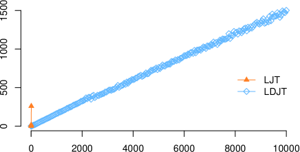
Figure 5: Runtimes [seconds], x-axis: maximum time steps

Now, we evaluate how long LDJT and LJT take to answer the queries for up to $10000$ time steps. Figure 5 shows the runtime in seconds for each maximum time step. We can see that the runtime of LDJT (diamond) to answer the questions is linear to the maximum number of time steps. Thus, LDJT more or less needs a constant time to answer queries once it instantiated the corresponding FO jtree and also the time to perform a forward or backward pass is more or less constant w.r.t. time, no matter how far LDJT already proceeded in time. For LDJT the runtimes for each operation are independent from the current time step, since the structure of the model stays the same over time. To be more precise, for our example LDJT takes about ${\sim}5$ms to initially construct the two FO jtrees. For a forward or backward pass, LDJT roughly needs ${\sim}6.5$ms. Both passes include a complete message pass, which roughly takes ${\sim}6$ms. Thus, most of the time for a forward or backward pass is spent on message passing. To answer a query, LDJT needs on average ${\sim}5$ms. To obtain the runtimes, we used a virtual machine having a 4 core Intel Xeon E5 with 2.4 GHz , 16 GB of RAM, and running Ubuntu 14.04.5 LTS (64 Bit).

Providing the unrolled model to LJT, it produces results for the first $8$ time steps with a reduced set of queries. Here, we can see that the runtime of LJT appears to be exponential to the maximum number of time steps, which is expected. The FO jtree construction of LJT is not optimised for the temporal case, such as creating an FO jtree similar to an unrolled version of LDJT’s FO jtree. Therefore, the number of PRVs in a parcluster increases with additional time steps in LJT. With additional time steps, the unrolled model becomes larger and while constructing an FO jtree, PRVs that depend on each other are more likely to be clustered in a parcluster. Thus, with more PRVs, the number of PRVs in a parcluster is expected to grow. In our example, maximum number of PRVs in a parcluster for $4$ time steps is $14$ and for $8$ time steps is $27$. For a ground jtree, the complexity of variable elimination is exponential to the largest cluster in the jtree (?). Thus, we can explain why LJT is more or less exponential to the maximum number of time steps.

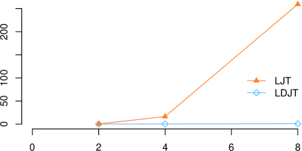
Figure 6: Runtimes [seconds], x-axis: maximum time steps

Overall, Fig. 5 shows (i) how crucial proper handling of temporal aspects is and (ii) that LDJT performs really well. Further, we can see that LDJT can handle combinations of different query types, such as smoothing and filtering. With evidence as input for all time steps the runtime is only marginally slower. Executing the example with evidence for all time steps produces an overhead of roughly ${\sim}8$ms on average for each time step. Therefore, for each time step, reinstantiating $10$ FO jtrees with evidence and performing message passing only produces an overhead of ${\sim}8$ms compared to having an empty set of evidence. The linear behaviour with increasing maximum time steps is the expected and desired behaviour for an algorithm handling temporal aspects. Furthermore, from a runtime complexity of LDJT there should be no difference in either performing a smoothing query with lag $10$ or a prediction query with $10$ time steps into the future. Thus, the previous results that LDJT outperforms the ground case still hold.

For the evaluation, the more time efficient version would be to always keep the last $10$ FO jtrees. Each message pass takes ${\sim}6$ms on average and during each backward pass LDJT performs a message pass. By keeping the instantiated FO jtrees, LDJT can halve the number of messages during a message passing. Assuming that the runtime of the message pass is linear to the number of calculated messages, resulting in reducing the runtime of each message pass to ${\sim}3$ms by keeping the FO jtrees. Further, for each time step, LDJT performs $10$ backward passes each with a message pass. Thus, LDJT can reduce the runtime by ${\sim}30$ms per time step and an overall reduce the runtime by ${\sim}300$s, which is about $20\%$ of the overall runtime for $10000$ timesteps.

7 Conclusion

We present a complete inter FO jtree backward pass for LDJT, allowing to perform smoothing efficiently for relational temporal models. LDJT answers multiple queries efficiently by reusing a compact FO jtree structure for multiple queries. Due to temporal m-separation, which is ensured by the in- and out-clusters, LDJT uses the same compact structure for all time steps $t>0$. Thus, LDJT also reuses the structure during a backward pass. Further, it reuses computations from a forward pass during a backward pass. LDJT’s relational forward backward pass also makes smoothing queries to the very beginning feasible. First results show that LDJT significantly outperforms LJT.

We currently work on extending LDJT to also calculate the most probable explanation as well as a solution to the maximum expected utility problem. The presented backward pass could also be helpful to deal with incrementally changing models. Additionally, it would be possible to reinstantiate an FO jtree for a backward pass solely given the $\alpha$ messages. Other interesting future work includes a tailored automatic learning for PDMs, parallelisation of LJT.

Acknowledgement

This research originated from the Big Data project being part of Joint Lab 1, funded by Cisco Systems, at the centre COPICOH, University of Lübeck

References

- [Ahmadi et al. 2013] Ahmadi, B.; Kersting, K.; Mladenov, M.; and Natarajan, S. 2013. Exploiting Symmetries for Scaling Loopy Belief Propagation and Relational Training. Machine learning 92(1):91–132.
- [Braun and Möller 2016] Braun, T., and Möller, R. 2016. Lifted Junction Tree Algorithm. In Proceedings of the Joint German/Austrian Conference on Artificial Intelligence (Künstliche Intelligenz), 30–42. Springer.
- [Braun and Möller 2017] Braun, T., and Möller, R. 2017. Preventing Groundings and Handling Evidence in the Lifted Junction Tree Algorithm. In Proceedings of the Joint German/Austrian Conference on Artificial Intelligence (Künstliche Intelligenz), 85–98. Springer.
- [Braun and Möller 2018] Braun, T., and Möller, R. 2018. Counting and Conjunctive Queries in the Lifted Junction Tree Algorithm. In Postproceedings of the 5th International Workshop on Graph Structures for Knowledge Representation and Reasoning, GKR 2017, Melbourne, Australia, August 21, 2017. Springer.
- [Darwiche 2009] Darwiche, A. 2009. Modeling and Reasoning with Bayesian Networks. Cambridge University Press.
- [de Salvo Braz 2007] de Salvo Braz, R. 2007. Lifted First-Order Probabilistic Inference. Ph.D. Dissertation, Ph. D. Dissertation, University of Illinois at Urbana Champaign.
- [Dignös, Böhlen, and Gamper 2012] Dignös, A.; Böhlen, M. H.; and Gamper, J. 2012. Temporal Alignment. In Proceedings of the 2012 ACM SIGMOD International Conference on Management of Data, 433–444. ACM.
- [Dylla, Miliaraki, and Theobald 2013] Dylla, M.; Miliaraki, I.; and Theobald, M. 2013. A Temporal-Probabilistic Database Model for Information Extraction. Proceedings of the VLDB Endowment 6(14):1810–1821.
- [Gehrke, Braun, and Möller 2018] Gehrke, M.; Braun, T.; and Möller, R. 2018. Lifted Dynamic Junction Tree Algorithm. In Proceedings of the 23rd International Conference on Conceptual Structures. Springer. [to appear].
- [Geier and Biundo 2011] Geier, T., and Biundo, S. 2011. Approximate Online Inference for Dynamic Markov Logic Networks. In Proceedings of the 23rd IEEE International Conference on Tools with Artificial Intelligence (ICTAI), 764–768. IEEE.
- [Lauritzen and Spiegelhalter 1988] Lauritzen, S. L., and Spiegelhalter, D. J. 1988. Local Computations with Probabilities on Graphical Structures and their Application to Expert Systems. Journal of the Royal Statistical Society. Series B (Methodological) 157–224.
- [Manfredotti 2009] Manfredotti, C. E. 2009. Modeling and Inference with Relational Dynamic Bayesian Networks. Ph.D. Dissertation, Ph. D. Dissertation, University of Milano-Bicocca.
- [Milch et al. 2008] Milch, B.; Zettlemoyer, L. S.; Kersting, K.; Haimes, M.; and Kaelbling, L. P. 2008. Lifted Probabilistic Inference with Counting Formulas. In Proceedings of AAAI, volume 8, 1062–1068.
- [Muñoz-González et al. 2017] Muñoz-González, L.; Sgandurra, D.; Barrere, M.; and Lupu, E. 2017. Exact Inference Techniques for the Analysis of Bayesian Attack Graphs. IEEE Transactions on Dependable and Secure Computing.
- [Murphy and Weiss 2001] Murphy, K., and Weiss, Y. 2001. The Factored Frontier Algorithm for Approximate Inference in DBNs. In Proceedings of the Seventeenth conference on Uncertainty in artificial intelligence, 378–385. Morgan Kaufmann Publishers Inc.
- [Murphy 2002] Murphy, K. P. 2002. Dynamic Bayesian Networks: Representation, Inference and Learning. Ph.D. Dissertation, University of California, Berkeley.
- [Nitti, De Laet, and De Raedt 2013] Nitti, D.; De Laet, T.; and De Raedt, L. 2013. A particle Filter for Hybrid Relational Domains. In Proceedings of the IEEE/RSJ International Conference on Intelligent Robots and Systems (IROS), 2764–2771. IEEE.
- [Özçep, Möller, and Neuenstadt 2015] Özçep, Özgür. L.; Möller, R.; and Neuenstadt, C. 2015. Stream-Query Compilation with Ontologies. In Proceedings of the 28th Australasian Joint Conference on Artificial Intelligence 2015 (AI 2015). Springer International Publishing.
- [Papai, Kautz, and Stefankovic 2012] Papai, T.; Kautz, H.; and Stefankovic, D. 2012. Slice Normalized Dynamic Markov Logic Networks. In Proceedings of the Advances in Neural Information Processing Systems, 1907–1915.
- [Poole 2003] Poole, D. 2003. First-order probabilistic inference. In Proceedings of IJCAI, volume 3, 985–991.
- [Richardson and Domingos 2006] Richardson, M., and Domingos, P. 2006. Markov Logic Networks. Machine learning 62(1):107–136.
- [Taghipour et al. 2013] Taghipour, N.; Fierens, D.; Davis, J.; and Blockeel, H. 2013. Lifted Variable Elimination: Decoupling the Operators from the Constraint Language. Journal of Artificial Intelligence Research 47(1):393–439.
- [Taghipour, Davis, and Blockeel 2013] Taghipour, N.; Davis, J.; and Blockeel, H. 2013. First-order Decomposition Trees. In Proceedings of the Advances in Neural Information Processing Systems, 1052–1060.
- [Thon, Landwehr, and De Raedt 2011] Thon, I.; Landwehr, N.; and De Raedt, L. 2011. Stochastic relational processes: Efficient inference and applications. Machine Learning 82(2):239–272.
- [Vlasselaer et al. 2014] Vlasselaer, J.; Meert, W.; Van den Broeck, G.; and De Raedt, L. 2014. Efficient Probabilistic Inference for Dynamic Relational Models. In Proceedings of the 13th AAAI Conference on Statistical Relational AI, AAAIWS’14-13, 131–132. AAAI Press.
- [Vlasselaer et al. 2016] Vlasselaer, J.; Van den Broeck, G.; Kimmig, A.; Meert, W.; and De Raedt, L. 2016. TP-Compilation for Inference in Probabilistic Logic Programs. International Journal of Approximate Reasoning 78:15–32.