Indirect inference through prediction

Abstract

By recasting indirect inference estimation as a prediction rather than a minimization and by using regularized regressions, we can bypass the three major problems of estimation: selecting the summary statistics, defining the distance function and minimizing it numerically. By substituting regression with classification we can extend this approach to model selection as well. We present three examples: a statistical fit, the parametrization of a simple real business cycle model and heuristics selection in a fishery agent-based model. The outcome is a method that automatically chooses summary statistics, weighs them and use them to parametrize models without running any direct minimization.

JEL Classification

C15; C63; C3

Keywords

Agent-based models; Indirect inference; Estimation; Calibration; Simulated minimum distance;

1 Introduction

We want to tune the parameters of a simulation model to match data. When the likelihood is intractable and the data high-dimensional, the common approach is the simulated minimum distance (Grazzini and Richiardi 2015). This involves summarising real and simulated data into a set of summary statistics and then tuning the model parameters to minimize their distance.

Minimization involves three tasks. First, choose the summary statistics. Second, weight their distance. Third, perform the numerical minimization keeping in mind that simulation may be computationally expensive.

Conveniently, “regression adjustment methods” from the approximate Bayesian computation(ABC) literature (Blum et al. 2013) can be adapted to side-step all 3 tasks. Moreover we can use these techniques outside of the ABC super-structure.

We substitute the minimization with a regression. First, run the model “many” times and observe pairs of model parameters and generated summary statistics. Then, regress the parameters as the dependent variable against all the simulated summary statistics. Finally, plug in the real summary statistics in the regression to obtain the tuned parameters. Model selection can be similarly achieved by training a classifier instead.

While the regressions can in principle be non-linear and/or non-parametric, we limit ourselves here to regularized linear regressions (the regularization is what selects the summary statistics). In essence, we can feed the regression a long list of summary statistics we think relevant and have the regularization select only what matters for parametrization.

We summarize the agent-based estimation in general and regression adjustment methods in particular in section 2. We describe how to parametrize models in section 3. We then provide 3 examples: a statistical line fit in section 4.1, a real business cycle macroeconomic model in section 4.2 and a fishery agent-based model in section 4.3. We conclude by pointing out weaknesses and possible extensions in section 5.

2 Literature review

The approach of condensing data and simulations into a set of summary statistics in order to match them is covered in detail in two review papers: Hartig et al. (2011) in ecology and Grazzini and Richiardi (2015) in economics.
They differ only in their definition of summary statistics: Hartig et al. (2011) defines it as any kind of observation available in both model and reality while Grazzini and Richiardi (2015), with its focus on consistency, allows only for statistical moments or auxiliary parameters from ergodic simulations.

Grazzini and Richiardi (2015) also introduces the catch-all term “simulated minimum distance” for a set of related estimation techniques, including indirect inference(Gourieroux, Monfort, and Renault 1993) and the simulated method of moments(McFadden 1989). Smith (1993) first introduced indirect inference to fit a 6-parameter real business cycle macroeconomic model.
In agent-based models, indirect inference was first advocated in Richiardi et al. (2006; see also Shalizi 2017) and first implemented in Zhao (2010) (who also proved mild conditions for consistency).

Common to all is the need to accomplish three tasks: selecting the summary statistics, defining the distance function and choosing how to minimize it.

Defining the distance function may at first appear the simplest of these tasks. It is standard to use the Euclidean distance between summary statistics weighed by the inverse of their variance or covariance matrix. However, while asymptotically efficient, this was shown to underperform in Smith (1993) and Altonji and Segal (1996). The distance function itself is a compromise, since in all but trivial problems we face a multi-objective optimization(see review by Marler and Arora 2004) where we should minimize the distance to each summary statistic independently. In theory, we could solve this by searching for an optimal Pareto front (see Badham et al. 2017 for an example of dominance analysis applied to agent-based models). In practice, however, even a small number of summary statistics make this approach infeasible and unintelligible. Better then to focus on a single imperfect distance function (a weighted global criterion, in multi-objective optimization terms) where there is at least the hope of effective minimization. A practical solution that may nonetheless obscure tradeoffs between summary statistic distances.

We can minimize distance function with off-the-shelf methods such as genetic algorithms (Calver and Hutzler 2006; Heppenstall, Evans, and Birkin 2007; Lee et al. 2015) or simulated annealing (Le et al. 2016; Zhao 2010). More recently two Bayesian frameworks have been prominent: BACCO (Bayesian Analysis of Computer Code Output) and ABC (Approximate Bayesian Computation).

BACCO involves running the model multiple times for random parameter inputs, building a statistical meta-model (sometimes called emulator or surrogate) predicting distance as a function of parameters and then minimizing the meta-model as a short-cut to minimizing the real distance. Kennedy and O’Hagan (2001) introduced the method(see O’Hagan 2006 for a review). Ciampaglia (2013), Parry et al. (2013) and Salle and Yıldızoğlu (2014) are recent agent-based model examples.

A variant of this approach interleaves running simulations and training the meta-model to sample more promising areas and achieve better minima. The general framework is the “optimization by model fitting”(see chapter 9 of Sean 2010 for a review; see Michalski 2000 for an early example). Lamperti, Roventini, and Sani (2018) provides an agent-based model application (using gradient trees as a meta-model). Bayesian optimization (see Shahriari et al. 2016 for a review) is the equivalent approach using Gaussian processes and Bailey et al. (2018) first applied it to agent-based models.

As in BACCO, ABC methods also start by sampling the parameter space at random but they only retain simulations whose distance is below a pre-specified threshold in order to build a posterior distribution of acceptable parameters(see Beaumont 2010 for a review). Drovandi, Pettitt, and Faddy (2011), Grazzini, Richiardi, and Tsionas (2017) and Zhang et al. (2017) apply the method to agent-based models. Zhang et al. (2017) notes that ABC matches the “pattern oriented modelling” framework of Grimm et al. (2005).

All these algorithms however require the user to select the summary statistics first. This is always an ad-hoc procedure. Beaumont (2010) describes it as “rather arbitrary” and notes that its effects “[have] not been systematically studied”. The more summary statistics we use, the more informative the simulated distance is (see Bruins et al. 2018 which compares four auxiliary models of increasing complexity). However the more summary statistics we use the harder the minimization (and the more important the weighting of individual distances) becomes.

Because of its use of kernel smoothing, ABC methods are particularly vulnerable to the “curse of dimensionality” with respect to the number of summary statistics. As a consequence the ABC literature has developed many “dimension reduction” techniques (see Blum et al. 2013 for a review). Of particular interest here is the “regression adjustment” literature (Beaumont, Zhang, and Balding 2002; Blum and Francois 2010; Nott et al. 2011) which advocates various ways to build regressions to map parameters from the summary statistics they generate. Our paper simplifies and applies this approach to agent-based models.

Model selection in agent-based models has received less attention. As in statistical learning one can select models on the basis of their out-of-sample predictive power (see Chapter 8 of Hastie, Tibshirani, and Friedman 2009). The challenge is then to develop a single measure to compare models of different complexity making multi-variate predictions. This has been fundamentally solved in Barde (2017) by using Markovian Information Criteria.
Our approach in section 3.2 differs from standard statistical model selection by treating it as a pattern recognition problem (that is, a classification), rather than making the choice based on ranking of out-of-sample prediction performance.

Fagiolo, Moneta, and Windrum (2007) were the first to tackle the growing variety of calibration methods in agent-based models. In the ensuing years, this variety has grown enormously. In the next section we add to this problem by proposing yet another estimation technique.

3 Method

3.1 Estimation

Take a simulation model depending on $K$ parameters $\theta=\left[\theta_{1},\theta_{2},\dots,\theta_{K}\right]$ to output $M$ simulated summary statistics $S(\theta)=\left[S_{1}(\theta),S_{2}(\theta),\dots,S_{M}(\theta)\right]$. Given real-world observed summary statistics $S^{*}$ we want to find the parameter vector $\theta^{*}$ that generated them.
Our method proceeds as follows:

1. Repeatedly run the model each time supplying it a random vector $\hat{\theta}$

2. Collect for each simulation its output as summary statistics $S(\hat{\theta})$

3. Run $K$ separate regularized regressions, $r_{i}$, one for each parameter. The parameter is the dependent variable and all the candidate summary statistics are independent variables:

   $$\left\{\begin{matrix}\theta_{1}=r_{1}(S_{1},S_{2},\dots,S_{M})\\ \theta_{2}=r_{2}(S_{1},S_{2},\dots,S_{M})\\ \vdots\\ \theta_{n}=r_{n}(S_{1},S_{2},\dots,S_{M})\end{matrix}\right.$$ (1)

4. Plug in the “real” summary statistics $S^{*}$ in each regression to predict the “real” parameters $\theta^{*}$

In step 1 and 2 we use the model to generate a data-set: we repeatedly input random parameters $\hat{\theta}$ and we collect the output $\hat{S}_{1},\dots,\hat{S}_{M}$ (see Table 1 for an example). In step 3 we take the data we generated and use it to train regressions (one for each model input) where we want to predict each model input $\theta$ looking only at the model output $S_{1},\dots,S_{M}$. The regressions map observed outputs back to the inputs that generated them.
Only in step 4 we use the real summary statistics (which we have ignored so far) to plug in the regressions we built in step 3. The prediction the regressions make when we feed in the real summary statistics $S^{*}$ are the estimated parameters $\theta^{*}$.

Table 1: A sample table generated after step 1 and 2 of the estimation procedure (assuming the simulation model depends on a single parameter $\theta_{1}$ ). Each row is a separate simulation run where $\hat{\theta}_{1}$ was the input of the model and $\hat{S}_{1},\dots,\hat{S}_{M}$ was its output. In step 3 we use this table to train a regression that uses as explanatory variables the output of the model $S_{1},\dots,S_{M}$ and try to predict from them the model input that generated them $\theta_{1}$

$\hat{\theta}_{1}$	$\hat{S}_{1}$	$\hat{S}_{2}$	$\dots$	$\hat{S}_{M}$
$\vdots$	$\vdots$	$\vdots$	$\vdots$	$\vdots$
$\vdots$	$\vdots$	$\vdots$	$\vdots$	$\vdots$

The key implementation detail is to use regularized regressions. We used elastic nets (Friedman, Hastie, and Tibshirani 2010) because they are linear and they combine the penalties of LASSO and ridge regressions. LASSO penalties automatically drop summary statistics that are uninformative. Ridge penalties lower the weight of summary statistics that are strongly correlated to each other.
We can then start with a large number of summary statistics (anything we think may matter and that the model can reproduce) and let the regression select only the useful ones. The regressions could also be made non-linear and non-parametric but this proved not necessary for our examples.

Compare this to simulated minimum distance. There, the mapping between model outputs $S(\cdot)$ and inputs $\theta$ is defined by the minimization of the distance function:

$$\theta^{*}=\arg_{\theta}\min(S(\theta)-S^{*})W(S(\theta)-S^{*})$$ (2)

When using a simulated minimum distance approach, both the summary statistics $S(\cdot)$ and their weights $W$ need to be chosen in advance. Then one can estimates $\theta^{*}$ by explicitly minimizing the distance. In effect the $\arg\min$ operator maps model output $S(\cdot)$ to model input $\theta$.
Instead, in our approach, the regularized regression not only selects and weights summary statistics but, more importantly, also maps them back to model input. Hence, the regression bypasses (takes the place of) the usual minimization.

3.2 Model Selection

We observe summary statistics $S^{*}$ from the real world and we would like to know which candidate model $\{m_{1},\dots,m_{n}\}$ generated them.
We can solve this problem by training a classifier against simulated data.

1. Repeatedly run each model

2. Collect for each simulation its generated summary statistics $S(m_{i})$

3. Build a classifier predicting the model by looking at summary statistics and train it on the data-set just produced:

   $$i\sim g(S_{1},S_{2},\dots,S_{M})$$ (3)

4. Plug in “real” summary statistics $S^{*}$ in the classifier to predict which model generated it

The classifier family $g(\cdot)$ can also be non-linear and non-parametric. We used a multinomial regression with elastic net regularization(Friedman, Hastie, and Tibshirani 2010); its advantages is that the regularization selects summary statistics and the output is a classic logit formula that is easily interpretable.

Model selection cannot be done on the same data-set used for estimation. If the parameters of a model need to be estimated, the estimation must be performed on on either a separate training data-set or the inner loop of a nested cross-validation(Hastie, Tibshirani, and Friedman 2009).

4 Examples

4.1 Fit Lines

4.1.1 Regression-based methods fit straight lines as well as ABC or Simulated Minimum Distance

In this section we present a simplified one-dimensional parametrization problem and show that regression methods perform as well as ABC and simulated minimum distance.

We observe 10 summary statistics (in this case these are just direct observations) $S^{*}=(S^{*}_{0},\dots,S^{*}_{9})$ and we assume they were generated by the model $S_{i}=\beta i+\epsilon$ where $\epsilon\sim\mathcal{N}(0,1)$. Assuming the model is correct, we want to estimate the $\beta^{*}$ parameter that generated the observed $S^{*}$. Because the model is a straight line, we could solve the estimation by least squares. Pretend however this model is a computational black box where the connection between it and drawing straight lines is not apparent.

We run 1,000 simulations with $\beta\sim U[0,2]$ (the range is arbitrary and could represent either a prior or a feasible interval), collecting the 10 simulated summary statistics $\hat{S}(\beta_{i})$. We then train a linear elastic net regression of the form:

$$\beta=a+\sum_{i=0}^{9}b_{i}\hat{S}_{i}$$ (4)

Table 2 shows the $b$ coefficients of the regression. $S_{0}$ contains no information about $\beta$ (since it is generated as $S_{0}=\epsilon$) and the regression correctly ignores it by dropping $b_{0}$. The elastic net weights larger summary statistics more because the effect of $\beta$ is larger there compared to the $\epsilon$ noise.

Table 2: Coefficients generated by fitting an elastic net against a training sample of size 1000. Notice that $b_{0}$ has been automatically dropped since in this case $S_{0}$ contains no information about $\beta$

Term	Estimate
(Intercept)	0.0297673
$b_{1}$	0.0010005
$b_{2}$	0.0065579
$b_{3}$	0.0056334
$b_{4}$	0.0109605
$b_{5}$	0.0134782
$b_{6}$	0.0190075
$b_{7}$	0.0203925
$b_{8}$	0.0238694
$b_{9}$	0.0281099

We test this regression by making it predict, out-of-sample, the $\beta$ of 1000 more simulations looking only at their summary statistics. Figure 1 and table 3 compare the estimation quality with those achieved by the standard rejection ABC and MCMC ABC (following Marjoram et al. 2003; Wegmann, Leuenberger, and Excoffier 2009; both methods implemented in Jabot et al. 2015). All achieve similar error rates.

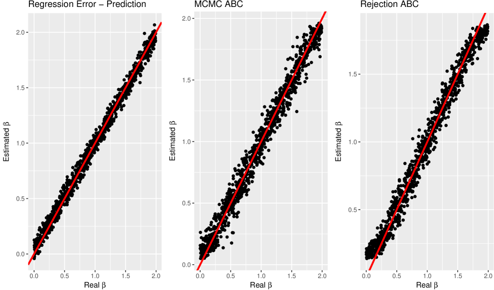
Figure 1: A side by side comparison between the ‘real’ and discovered $\beta$ as generated by either the regression method or two standard ABC algorithms: rejection sampling or MCMC. The x-axis represents the real $\beta$, the y-axis its estimate. Each point represents the estimation against a different set of summary statistics. The red line is the 45 degree line: the closer the points are to it the better the estimation. All methods perform equally well.

Table 3: All three methods achieve on average similar estimation errors, although the regression-based method is much quicker

Estimation	Average RMSE	Runtime	Runtime(scaled)
Regression Method	0.0532724	0.002239561 mins	1.0000
Rejection ABC	0.0823950	0.9586897 mins	428.0703
MCMC ABC	0.0835164	5.453199 mins	2434.9408

We can also compare the regression against the standard simulated minimum distance approach. Simulated minimum distance search for the parameters that minimize:

$$\beta^{*}=\arg_{\beta}\min(S(\beta)-S^{*})W(S(\beta)-S^{*})$$ (5)

The steeper its curvature, the easier it is to minimize numerically.
In figure 2 we compare the curvature defined by $W=I$ and $W=\left(\text{diag}(\Sigma)\right)^{-1}$ (where $I$ is the identity matrix and $\Sigma$ is the covariance matrix of summary statistics) against the curvature implied by our regression $r$: $|r(S^{*})-r(S)|$ (that is, the distance between the estimation made given the real summary statistics, $r(S^{*})$, and the estimation made at other simulated summary statistics $r(S)$) . This problem is simple enough that the usual weight matrices produce distance functions that are easy to numerically minimize.

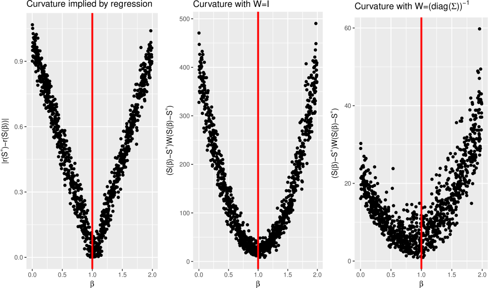
Figure 2: Curvature of the fitness function as implied by the regression versus weighted Euclidean distance between summary statistics. We take the 1000 testing simulation runs, we pick one in the middle ($\beta\approx 1$) as the ‘real’ one and we compute the summary statistics distances between all the other simulations to it. The red line represents the real $\beta$, each dot is the distance to the real $\beta$ for that simulation run and its associated $\beta$.

We showed here that regression-based methods perform as well as ABC and simulated minimum distance in a simple one-dimensional problem.

4.1.2 Regression-based methods fit broken lines better than ABC or simulated minimum distance

In this section we present another simplified one-dimensional parametrization but show that regression methods outperform both ABC and simulated minimum distance because of better selection of summary statistics.

We observe 10 summary statistics $S=(S_{0},\dots,S_{9})$ but we assume they were generated by the “broken line” model:

$$S_{i}=\left\{\begin{matrix}\epsilon&i<5\\ \beta i+\epsilon&i\geq 5\end{matrix}\right.$$ (6)

where $\epsilon\sim\mathcal{N}(0,1)$.
We want to find the $\beta$ that generated the observed summary statistics. Notice that $S_{0},\dots,S_{4}$ provide no information on $\beta$.

As before we run the model 1000 times to train an elastic net of the form:

$$\beta=a+\sum_{i=0}^{9}b_{i}S_{i}$$ (7)

Table 4 shows the coefficients found. The regression correctly drops $b_{0},\dots,b_{4}$ and weighs the remaining summary statistics more the higher they are.

We run the model another 1000 times to test the regression ability to estimate their $\beta$. As shown in Figure 3 and Table 5 the regression outperforms both ABC alternatives. This is due to the elastic net ability to prune unimportant summary statistics.

Table 4: Coefficient estimates after 1000 training observations; notice that all the uninformative summary statistics have been automatically dropped.

Term	Estimate
(Intercept)	0.0360036
$b_{5}$	0.0189285
$b_{6}$	0.0202486
$b_{7}$	0.0222020
$b_{8}$	0.0288608
$b_{9}$	0.0273448

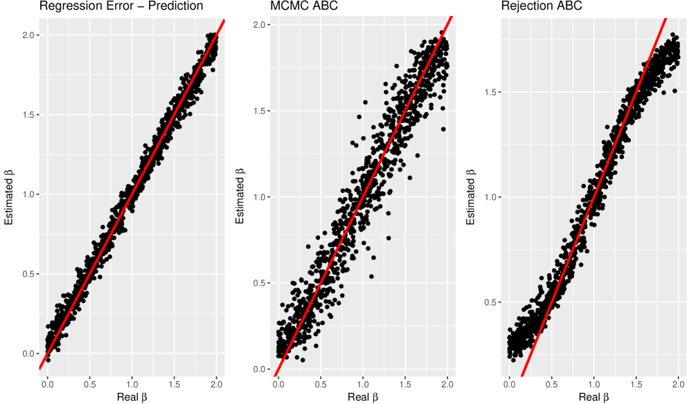
Figure 3: A side by side comparison between the ‘real’ and discovered $\beta$ as generated by either the regression method or two standard ABC algorithms: rejection sampling or MCMC. The x-axis represents the real $\beta$, the y-axis its estimate. Each point represents the estimation against a different set of summary statistics. The red line is the 45 degree line: the closer the points are to it the better the estimation. Notice that rejection sampling (ABC) is inaccurate when $\beta$ is very small (near 0) or very large (near 2) while MCMC has a larger average error than regression-based methods

Table 5: Regression errors achieve lower estimation errors in a fraction of the time. This is because they automatically ignore all summary statistics that do not inform $\beta$

Estimation	Average RMSE	Runtime	Runtime(scaled)
Regression Method	0.0579736	0.0008367697 mins	1.000
Rejection ABC	0.1278042	0.9592413 mins	1146.362
MCMC ABC	0.1343737	6.273226 mins	7496.956

In simulated minimum distance methods, choosing the wrong $W$ can compound the problem of poor summary statistics selection. As shown in Figure 4 the default choice $W=\left(\text{diag}(\Sigma)\right)^{-1}$ detrimentally affects the curvature of the distance function, by adding noise. This is because summary statistics $S_{0},\dots,S_{4}$, in spite of containing no useful information, are the values with the lowest variance and are therefore given larger weights.

Figure 4: Curvature of the fitness function as implied by the regression versus weighted Euclidean distance between summary statistics. We take the 1000 training simulation runs, we pick one in the middle ($\beta\approx 1$) as the ‘real’ one and we compute the summary statistics distances between all the other simulations to it. The red line represents the real $\beta$, each dot is the distance to the real $\beta$ for that simulation run and its associated $\beta$. For this model the default choice of weighing matrix (the inverse of the variance diagonal) makes numerical minimization harder.

We showed here how, even in a simple one dimensional problem, the ability to prune uninformative summary statistics will result in better estimation (as shown by RMSE in table 5) .

4.1.3 Model selection through regression-based methods is informative and accurate

In this section we train a classifier to choose which of the two models we described above (‘straight-’ and ‘broken-line’) generated the observed data. We show that the classifier does a better job than choosing the model that minimizes prediction errors.

We observe 10 summary statistics $S^{*}=(S^{*}_{0},\dots,S^{*}_{9})$ and we would like to know if they were generated by the “straight-line” model:

$$S_{i}=\beta i+\epsilon$$ (8)

or the “broken-line” model:

$$S_{i}=\left\{\begin{matrix}\epsilon&i<5\\ \beta i+\epsilon&i\geq 5\end{matrix}\right.$$ (9)

where $\epsilon\sim N(0,1)$ and $i\in[0,9]$. Assume we have already estimated both models and $\beta=1$.

We run each model 1000 times and then train a logit classifier:

$$\text{Pr}(\text{broken line model})=\frac{1}{1+\exp(-[a+\sum b_{i}S_{i}])}$$ (10)

Notice that $S_{0}$ and $S_{5},\dots,S_{9}$ are generated by the same rule in both models: both draw a straight line through those points. Their values will then not be useful for model selection. We should focus instead exclusively on $S_{1},\dots,S_{4}$ since that is the only area where one model draws a straight line and the other does not.
The regularized regression discovers this, by dropping $b_{0}$ and $b_{5},\dots,b_{9}$ as Table 6 shows.

Table 6: Coefficient estimates after 2000 training observations; notice how only the low summary statistics have a coefficient associated to them. This is because they are the only part of the line that is ’broken’: $S_{5},\dots,S_{9}$ are generated the same way for both models and are therefore of no use for differentiating the two models.

Term	Estimate
(Intercept)	-11.1578231
$b_{1}$	0.5733553
$b_{2}$	1.1016989
$b_{3}$	2.0715734
$b_{4}$	1.8777375

Figure 5 tabulates the success rate from 2000 out-of-sample simulations by the classifier and compares it with picking models by choosing the one that minimizes the distance between summary statistics. The problem is simple enough that choosing $W=I$ achieves almost perfect success rate; using the more common variance-based weights does not.

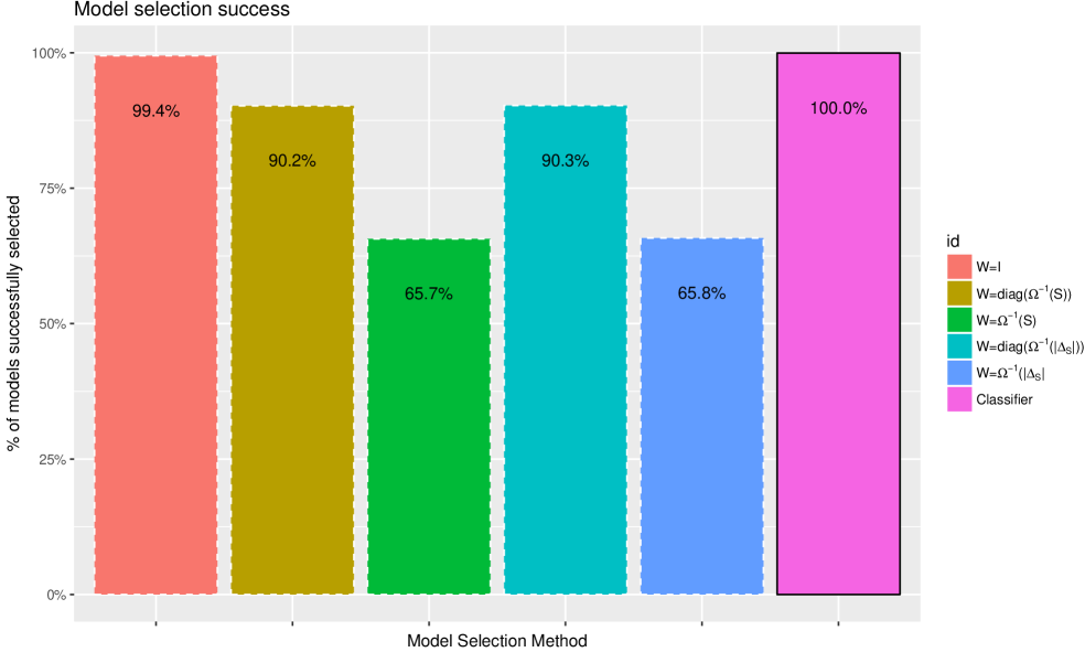
Figure 5: A comparison between training a classifier to do model selection versus choosing the model whose distance to summary statistics is smaller. All weighing schemes except $W=I$ underperform compared to the classifier. Model selection performed on 2000 testing runs (not used for training the classifier)

4.2 Fit RBC

4.2.1 Fit against cross-correlation matrix

In this section we parametrize a simple macro-economic model by looking at the time series it simulates. We show that we can use a large number of summary statistics efficiently and that we can diagnose estimation strengths and weaknesses the same way we diagnose regression outputs.

We observe 150 steps of 5 quarterly time series: $Y,r,I,C,L$. Assuming we know they come from a standard real business cycle (RBC) model (the default RBC implementation of the gEcon package in R, see Klima, Podemski, and Retkiewicz-Wijtiwiak 2018, see also Appendix A), we estimate the 6 parameters ($\beta,\delta,\eta,\mu,\phi,\sigma$) that generated them.

Summarize the time series observed with (a) the $t=-5,\dots,+5$ cross-correlation vectors of $Y$ against $r,I,C,L$, (b) the lower-triangular covariance matrix of $Y,r,I,C,L$, (c) the squares of all cross-correlations and covariances, (d) the pair-wise products between all cross-correlations and covariances. This totals to 2486 summary statistics: too many for most ABC approaches.
This problem is however still solvable by regression. We train 6 separate regressions, one for each parameter, as follows:

$$\left\{\begin{matrix}\beta&=\sum a_{\beta,i}S_{i}+\sum b_{\beta,i}S_{i}^{2}+\sum c_{\beta,i,j}S_{i}S_{j}\\ \gamma&=\sum a_{\gamma,i}S_{i}+\sum b_{\gamma,i}S_{i}^{2}+\sum c_{\gamma,i,j}S_{i}S_{j}\\ &\vdots\\ \sigma&=\sum a_{\sigma,i}S_{i}+\sum b_{\sigma,i}S_{i}^{2}+\sum c_{\sigma,i,j}S_{i}S_{j}\\ \end{matrix}\right.$$ (11)

Where $a,b,c$ are elastic net coefficients.

We train the regressions over 2000 RBC runs then produce 2000 more to test its estimation. Figure 6 and Table 7 show that all the parameters are estimated correctly but $\eta$ and $\delta$ less precisely than the others. We judge the quality of the estimation through the predictivity coefficient (see Salle and Yıldızoğlu 2014; also known as modelling efficiency as in Stow et al. 2009) which measures the improvement of using an estimate $\hat{\beta}$ to discover the real $\beta^{*}$ as opposed to just using the hindsight average $\bar{\beta}$:

$$\text{Predictivity}=\frac{\sum\left(\beta^{*}_{i}-\bar{\beta}\right)^{2}-\sum\left(\beta^{*}_{i}-\hat{\beta}_{i}\right)^{2}}{\sum\left(\beta^{*}_{i}-\bar{\beta}\right)^{2}}$$ (12)

Intuitively, this is just an extension of the definition to $R^{2}$ to out-of-sample predictions. A predictivity of 1 implies perfect estimation, 0 implies that averaging would have performed as well as the estimate.

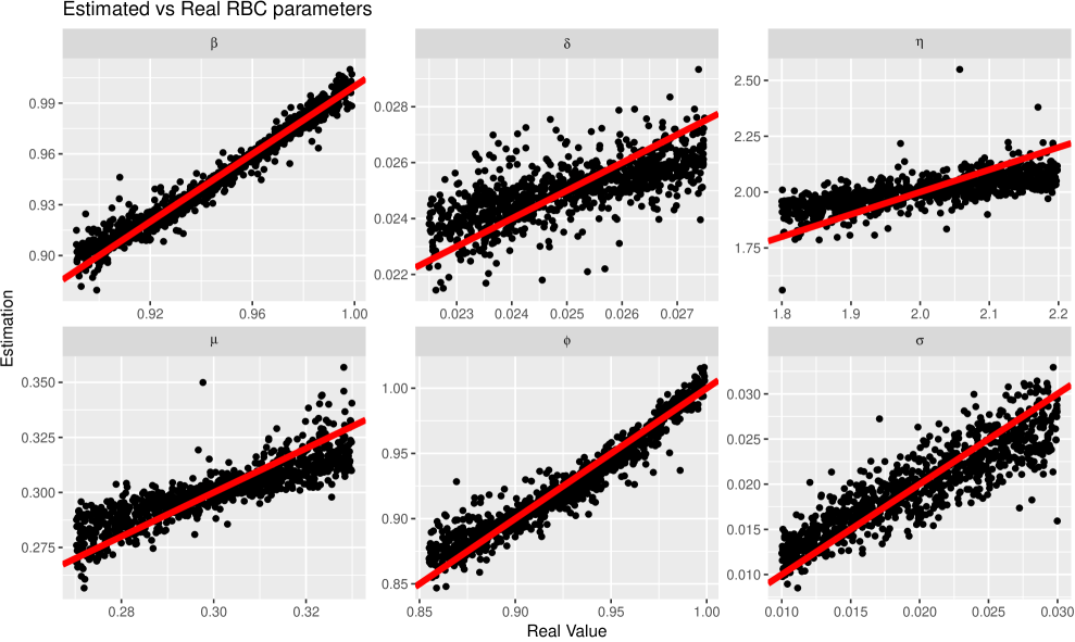
Figure 6: Estimated versus real parameters for 2000 RBC runs in the testing data-set (not used for training the regressions). Each dot is a pair real-estimate parameter from a single RBC run. Red line is the 45 degree line: the closer the dots are to it the better estimated that parameter is. The parameters $\delta$ and $\eta$ are not as well estimated as the other 4

Table 7: Predictivity for each variable when estimating parameters of the RBC model looking at cross-correlations and covariance; $\delta$ and $\eta$ are less precisely estimated than the other parameters. All results obtained on a testing data-set (not used for training) of 2000 RBC runs. Bias is defined as average distance between real and estimated parameter: $\theta^{*}-\theta$, RMSE is the root mean square error: $\sqrt{\sum\frac{\left(\theta^{*}-\theta\right)^{2}}{2000}}$. Variable bounds are the interval 20% below and above the default RBC parameters in the original gEcon implementation.

Variable	Variable Bounds	Average Bias	Average RMSE	Predictivity
$\beta$	[0.891,0.999]	0.0003105	0.0000351	0.9635677
$\delta$	[0.225,0.275]	-0.0000426	0.0000010	0.4997108
$\eta$	[1.8,2.2]	-0.0009051	0.0062672	0.5168588
$\mu$	[0.27,0.33]	0.0001315	0.0000774	0.7419450
$\sigma$	[0.01,0.03]	-0.0000391	0.0000071	0.7941670
$\phi$	[0.855,0.999]	-0.0001568	0.0001203	0.9265618

We showed here that we can estimate the parameters of a simple RBC model by looking at their cross-correlations. However this method is better served by looking at multiple auxiliary models as we show in the next section.

4.2.2 Fit against auxiliary fits

In this section we parametrize the same simple macro-economic model by looking at the same time series it simulates but using a more diverse array of summary statistics. We show how that improves the estimation of the model.

Again, we observe 150 steps of 5 quarterly time series: $Y,r,I,C,L$. Assuming we know they come from a standard RBC model, we want to estimate the 6 parameters ($\beta,\delta,\eta,\mu,\phi,\sigma$) that generated them.

In this section we use a larger variety of summary statistics. Even though they derive from auxiliary models that convey much of the same information, we are able to use them efficiently for estimation. We summarize output by (i) coefficients of regressing $Y$ on $Y_{t-1},I_{t},I_{t-1}$, (ii) coefficients of regressing $Y$ on $Y_{t-1},C_{t},C_{t-1}$, (iii) coefficients of regressing $Y$ on $Y_{t-1},r_{t},r_{t-1}$, (iv) coefficients of regressing $Y$ on $Y_{t-1},L_{t},L_{t-1}$, (v) coefficients of regressing $Y$ on $C,r$ (vi) coefficients of fitting AR(5) on $Y$, (vii) the (lower triangular) covariance matrix of $Y,I,C,r,L$.
In total there are 48 summary statistics to which we add all their squares and cross-products.

Again we train 6 regressions against 2000 RBC observations and test their estimation against 2000 more.
Figure 7 and Table 8 shows that all the parameters are estimated correctly and with higher predictivity coefficient. In particular $\delta$ and $\eta$ are better predicted than by looking at cross-correlations.

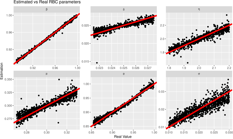
Figure 7: Estimated versus real parameters for 2000 RBC runs in the testing data-set (not used for training the regressions). Each dot is a pair of real-estimate parameters from a single RBC run. The red line is the 45 degree line: the closer the dots are to it the better estimated that parameter is. All parameters are well estimated

Table 8: Predictivity for each variable when estimating parameters of the RBC model looking at cross-correlations and covariance; All parameters are well estimated. All results obtained on a testing data-set (not used for training) of 2000 RBC runs. Bias is defined as average distance between real and estimated parameter: $\theta^{*}-\theta$, RMSE is the root mean square error: $\sqrt{\sum\frac{\left(\theta^{*}-\theta\right)^{2}}{2000}}$. Variable bounds are the interval 20% below and above the default RBC parameters in the original gEcon implementation.

Variable	Variable Bounds	Average Bias	Average RMSE	Predictivity
$\beta$	[0.891,0.999]	0.0000154	0.0000023	0.9975601
$\delta$	[0.225,0.275]	-0.0000308	0.0000003	0.8285072
$\eta$	[1.8,2.2]	0.0001992	0.0012552	0.9040992
$\mu$	[0.27,0.33]	0.0000126	0.0000357	0.8793255
$\sigma$	[0.01,0.03]	-0.0000638	0.0000061	0.8100463
$\phi$	[0.855,0.999]	0.0002740	0.0000244	0.9862208

4.3 Heuristic selection in the face of input uncertainty

In this section we select between 10 variations of an agent-based model where some inputs and parameters are unknowable. By training a classifier we are able to discover which summary statistics are robust to the unknown parameters and leverage this to outperform standard model selection by prediction error.

Assume all fishermen in the world can be described by one of 10 decision-making algorithms (heuristics). We observe 100 fishermen for five years and we want to identify which heuristic they are using. The heuristic selection is however complicated by not knowing basic biological facts about the environment the fishermen exploit.
This is a common scenario in fisheries: we can monitor boats precisely through electronic logbooks and satellites but more than 80% of global catch comes from unmeasured fish stocks(Costello et al. 2012).
Because heuristics are adaptive, the same heuristic will generate very different summary statistics when facing different biological constraints. We show here that we can still identify heuristics even without knowing how many fish there are in the sea.

We can treat each heuristic as a separate model and train a classifier that looks at summary statistics to predict which heuristic generated them. The critical step is to train the classifier on example runs where the uncertain inputs (the unknown biological constraints) are randomized. This way the classifier automatically learns which summary statistics are robust to biological changes and look only at those when selecting the right heuristic.

We use POSEIDON(Bailey et al. 2018), a fishery agent-based model to simulate the fishery. We observe the fishery for five years and we collect 17 summary statistics: (i) aggregate five year averages on landings, effort (hours spent fishing), distance travelled from port, number of trips per year and average hours at sea per trip, (ii) a discretized(3 by 3 matrix) heatmap of geographical effort over the simulated ocean, (iii) the coefficients and $R^{2}$ of a discrete choice model fitting area fished as a function of distance from port and habit (an integer describing how many times that particular fisher has visited that area before in the past 365 days ).
These summary statistics are a typical information set we might expect to obtain in a developed fishery.

Within each simulation, all fishers use the same heuristic. There are 10 possible candidates,all described more in depth in a separate paper:

• Random: each fisher each trip picks a random cell to trawl

• Gravitational Search: agents copy one another as if planets attracted by gravity where mass is equal to profits made in the previous trip (see Rashedi, Nezamabadi-pour, and Saryazdi 2009)

• $\epsilon$-greedy bandit: agents have a fixed 20% chance of exploring a new random area otherwise exploiting(fishing) the currently most profitable discovered location. Two parametrizations of this heuristic are available, depending on whether fishers discretize the map in a 3 by 3 matrix or a 9 by 9 one.

• “Perfect” agent: agents knows perfectly the profitability of each area $\Pi(\cdot)$ and chooses to fish in area $i$ by SOFTMAX:

  $$\text{Probability}(i)=\frac{e^{\Pi(i)}}{\sum_{j}e^{\Pi(j)}}$$ (13)

• Social Annealing: agents always return to the same location unless they are making less than fishery’s average profits(across the whole fishery), in which case they try a new area at random

• Explore-Exploit-Imitate: like $\epsilon$-greedy agents, they have a fixed probability of exploring. When not exploring each fisher checks the profits of two random “friends” and copies their location if either are doing better. Three parametrizations of this heuristics are possible: exploration rate at 80% or 20% with exploration range of 5 cells, or 20% exploration rate with exploration range of 20 cells.

• Nearest Neighbour: agents keep track of the profitability of all the areas they have visited through a nearest neighbour regression and always fish the peak area predicted by the regression.

All runs are simulations of the single-species “baseline” fishery described in the ESM of Bailey et al. (2018) (see also Appendix B).
We run the model 10,000 times in total, 1000 times for each heuristic. We also randomize in each simulation three biological parameters: (i) carrying capacity of the each cell map, (ii) diffusion speed of fish, (iii) the Malthusian growth parameter of the stock.

We train a multi-logit classifier on the simulation outputs as shown in section 3.2:

$$\text{Pr}(\text{Heuristic }i)=\frac{e^{b_{i}^{\prime}S}}{1+\sum_{j}e^{b_{j}^{\prime}S}}$$ (14)

where $b_{1},\dots,b_{10}$ are vectors of elastic net coefficients.

We build the testing data-set by running the model 10,000 more times. We compare the quality of model selection against selection by weighted prediction error.
First, in Figure 8 the prediction error is computed by re-running simulations with the correct random biological parameters. In spite of having a knowledge advantage over the classifier, selection by prediction error performs worse than the classifier. In Figure 9 we do not assume to know the random biological parameters. Prediction error (which now tries to minimize the distance between simulations which differ in both heuristics and biological parameters) performs much worse.

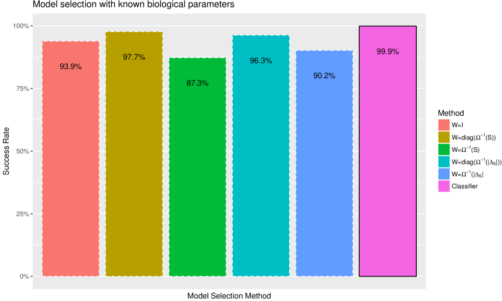
Figure 8: Comparison of success rate in correctly estimating which heuristics generated a given summary statistics $S$. The classifier success rate has solid borders. In this set of simulations model selection by minimum prediction error is advantaged by knowing the correct biological parameters while the classifier is a single global model trained over all combinations of biological parameters.

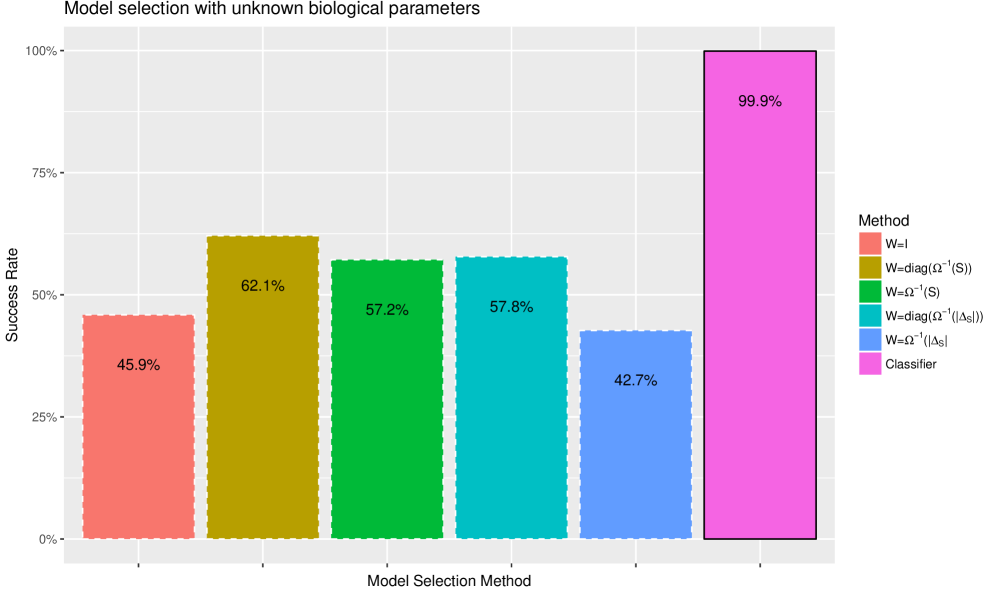
Figure 9: Comparison of success rate in correctly estimating which heuristics generated a given summary statistics $S$. The classifier success rate has solid borders. In this set of simulations model selection by minimum prediction error has no additional knowledge about the biological parameters.

Model selection by prediction error is hard if we are not certain about all model inputs. However it is trivial to train a classifier by feeding it observations from different parameter configurations such that only the summary statistics “robust” to such parameter noise are used for model selection.

5 Discussion

5.1 Advantages of a regression-based approach

Regression are commonly-used and well-understood. We leverage that knowledge for parameter estimation.
By looking at out-of-sample prediction we can immediately diagnose parameter identification problems: the lower the accuracy, the weaker the identification (compare this to diagnosis of numerical minimization outputs as in Canova and Sala 2009) . Moreover, if the regression is linear, its coefficients show which summary statistic $S_{i}$ inform which model parameter $\theta_{i}$.

A secondary advantage of building a statistical model is the ease with which additional input uncertainty can be incorporated as shown in section 4.3. If we are uncertain about an input and cannot estimate it directly (because of lack of data or under-identification), it is straightforward to simulate for multiple values of the input, train a statistical model and then check whether it is possible to estimate reliably the other parameters. In a simulated minimum distance setting we would have to commit to a specific guess of the uncertain input before running a minimization or minimize multiple times for each guess (without any assurance that the weighing matrix ought to be kept constant between guesses).

5.2 Weaknesses

This method has two main limits. First, users cannot weight summary statistics by importance. As a consequence, the method cannot be directed to replicate a specific summary statistic. Imagine a financial model of the housing market which we may judge primarily by its ability of matching real house prices. However, when estimating its parameters the regression may ignore house prices entirely and focus on another seemingly minor summary statistic (say, total number of bathrooms). While that may be an interesting and useful way of parametrizing the model, it does not guarantee a good match with observed house prices.
Nevertheless, in this case one option would be to transition to a weighted regression and weigh more the observations whose generated summary statistic $S_{i}$ were close to the value of $S_{i}^{*}$ we are primarily interested in replicating. As such, the model would be forced to include component deemed important, even if not the most efficient in terms of explanatory power. Comparing this fit with the unweighted one may also be instructive.

The second limit is that the each parameter is estimated separately. Because each parameter is given a separate regression, this method may underestimate underlying connections (dependencies) between two or more parameters when such connections are not reflected in changes to summary statistics. This issue is mentioned in the ABC literature by Beaumont (2010) although it is also claimed that in practice it does not seem to be an issue. It may however be more appropriate to use a simultaneous system estimation routine(Henningsen and Hamann 2007) or a multi-task learning algorithm(Evgeniou and Pontil 2004).

5.3 Possible Extensions

Our method contains a fundamental inefficiency: we build a global statistical model to use only once when plugging in the real summary statistics $S^{*}$. Given that the real summary statistics $S^{*}$ are known in advance, a direct search ought to be more efficient.
Our method makes up for this by solving multiple problems at once as it implicitly selects summary statistics and weights them while estimating the model parameters.

In machine learning, transduction substitutes regression when we are interested in a prediction for a known $S^{*}$ only, without the need to build a global statistical model(see Chapter 10 of Cherkassky and Mulier 2007; Beaumont, Zhang, and Balding 2002 weights simulations depending on the distance to known $S^{*}$ in essentially the same approach). Switching to transduction would however remove the familiarity advantage of using regressions as well as the ease to test its predictive power with randomly generated summary statistics.

Another avenue for improvement is to use non-linear, non-parametric regressions. Blum and Francois (2010) used neural networks, for example. Non-parametrics are more flexible but they may be more computationally demanding and their final output harder to interpret.

It may also be possible to use regressions as an intermediate step in a more traditional simulated minimum distance problem. We would still build a regression for each parameter but then using them as the distance function to minimize by standard numerical methods.

5.4 Conclusion

We presented here a general method to fit agent-based and simulation models. We perform indirect inference using prediction rather than minimization, and, by using regularized regressions, we avoid three major problems of estimation: selecting the most valuable of the summary statistics, defining the distance function, and achieving reliable numerical minimization. By substituting regression with classification we can further extend this approach to model selection. This approach is relatively easy to understand and apply, and at its core uses statistical tools already familiar to social scientists. The method scales well with the complexity of the underlying problem, and as such may find broad application.

Appendix A: RBC Model

Consumer

$$\max_{K^{\mathrm{s}}_{t},C_{t},L^{\mathrm{s}}_{t},I_{t}}U_{t}={\beta}{\mathrm{E}_{t}\left[U_{t+1}\right]}+\left(1-\eta\right)^{-1}{\left({{C_{t}}^{\mu}}{\left(1-L^{\mathrm{s}}_{t}\right)^{1-\mu}}\right)^{1-\eta}}$$ (15)

$$C_{t}+I_{t}=\pi_{t}+{K^{\mathrm{s}}_{t-1}}{r_{t}}+{L^{\mathrm{s}}_{t}}{W_{t}}$$ (16)

$$K^{\mathrm{s}}_{t}=I_{t}+{K^{\mathrm{s}}_{t-1}}\left(1-\delta\right)$$ (17)

Firm

$$\max_{K^{\mathrm{d}}_{t},L^{\mathrm{d}}_{t},Y_{t}}\pi_{t}=Y_{t}-{L^{\mathrm{d}}_{t}}{W_{t}}-{r_{t}}{K^{\mathrm{d}}_{t}}$$ (18)

$$Y_{t}={Z_{t}}{{K^{\mathrm{d}}_{t}}^{\alpha}}{{L^{\mathrm{d}}_{t}}^{1-\alpha}}$$ (19)

Equilibrium

$$K^{\mathrm{d}}_{t}=K^{\mathrm{s}}_{t-1}$$ (20)

$$L^{\mathrm{d}}_{t}=L^{\mathrm{s}}_{t}$$ (21)

$$Z_{t}=e^{\epsilon^{\mathrm{Z}}_{t}+{\phi}{\log{Z_{t-1}}}}$$ (22)

$$-0.36Y_{\mathrm{ss}}+{r_{\mathrm{ss}}}{K^{\mathrm{s}}_{\mathrm{ss}}}=0$$ (23)

Appendix B: Fishery Parameters

Parameter	Value	Meaning
Biology	Logistic
$K$	$\sim U[1000,10000]$	max units of fish per cell
$m$	$\sim U[0,0.003]$	fish speed
$r$	$\sim U[.3,.8]$	Malthusian growth parameter
Fisher	Explore-Exploit-Imitate
rest hours	12	rest at ports in hours
$\epsilon$	0.2	exploration rate
$\delta$	$\sim U[1,10]$	exploration area size
fishers	100	number of fishers
friendships	2	number of friends each fisher has
max days at sea	5	time after which boats must come home
Map
width	50	map size horizontally
height	50	map size vertically
port position	40,25	location of port
cell width	10	width (and height) of each cell map
Market
market price	10	$ per unit of fish sold
gas price	0.01	$ per litre of gas
Gear
catchability	0.01	% biomass caught per tow hour
speed	5.0	distance/h of boat
hold size	100	max units of fish storable in boat
litres per unit of distance	10	litres consumed per distance travelled
litres per trawling hour	5	litres consumed per hour trawled

References

Altonji, Joseph G., and Lewis M. Segal. 1996. “Small-Sample Bias in GMM Estimation of Covariance Structures.” Journal of Business & Economic Statistics 14 (3). Taylor & Francis, Ltd.American Statistical Association:353. https://doi.org/10.2307/1392447.

Badham, Jennifer, Chipp Jansen, Nigel Shardlow, and Thomas French. 2017. “Calibrating with Multiple Criteria: A Demonstration of Dominance.” Journal of Artificial Societies and Social Simulation 20 (2). JASSS:11. https://doi.org/10.18564/jasss.3212.

Bailey, R, Ernesto Carrella, Robert Axtell, M Burgess, R Cabral, Michael Drexler, Chris Dorsett, J Madsen, Andreas Merkl, and Steven Saul. 2018. “A computational approach to managing coupled human-environmental systems: the POSEIDON model of ocean fisheries.” Sustainability Science, June. Springer Japan, 1–17. https://doi.org/10.1007/s11625-018-0579-9.

Barde, Sylvain. 2017. “A Practical, Accurate, Information Criterion for Nth Order Markov Processes.” Computational Economics 50 (2). Springer US:281–324. https://doi.org/10.1007/s10614-016-9617-9.

Beaumont, Mark A. 2010. “Approximate Bayesian Computation in Evolution and Ecology.” Annual Review of Ecology, Evolution, and Systematics 41 (1):379–406. https://doi.org/10.1146/annurev-ecolsys-102209-144621.

Beaumont, Mark A, Wenyang Zhang, and David J Balding. 2002. “Approximate Bayesian computation in population genetics.” Genetics 162 (4):2025–35. https://doi.org/Genetics December 1, 2002 vol. 162 no. 4 2025-2035.

Blum, M G B, M A Nunes, D Prangle, and S A Sisson. 2013. “A comparative review of dimension reduction methods in approximate Bayesian computation.” Statistical Science 28 (2):189–208. https://doi.org/10.1214/12-STS406.

Blum, Michael G B, and Olivier Francois. 2010. “Non-linear regression models for Approximate Bayesian Computation.” Statistics and Computing 20 (1):63–73. https://doi.org/10.1007/s11222-009-9116-0.

Bruins, Marianne, James A Duffy, Michael P Keane, and Anthony A Smith. 2018. “Generalized indirect inference for discrete choice models.” Journal of Econometrics 205 (1):177–203. https://doi.org/10.1016/j.jeconom.2018.03.010.

Calver, Benoit, and Guillaume Hutzler. 2006. “Automatic Tuning of Agent-Based Models Using Genetic Algorithms.” In Lecture Notes in Computer Science, 3891:41–57. Springer, Berlin, Heidelberg. https://doi.org/10.1007/11734680.

Canova, Fabio, and Luca Sala. 2009. “Back to square one: Identification issues in DSGE models.” Journal of Monetary Economics 56 (4):431–49. https://doi.org/10.1016/j.jmoneco.2009.03.014.

Cherkassky, Vladimir S., and Filip. Mulier. 2007. Learning from data : concepts, theory, and methods. IEEE Press. https://www.wiley.com/en-gb/Learning+from+Data:+Concepts,+Theory,+and+Methods,+2nd+Edition-p-9780471681823.

Ciampaglia, Giovanni Luca. 2013. “A framework for the calibration of social simulation models.” Advances in Complex Systems 16 (04n05). World Scientific Publishing Company:1350030. https://doi.org/10.1142/S0219525913500306.

Costello, Christopher, Daniel Ovando, Ray Hilborn, Steven D. Gaines, Olivier Deschenes, and Sarah E. Lester. 2012. “Status and solutions for the world’s unassessed fisheries.” Science 338 (6106):517–20. https://doi.org/10.1126/science.1223389.

Drovandi, Christopher C., Anthony N. Pettitt, and Malcolm J. Faddy. 2011. “Approximate Bayesian computation using indirect inference.” Journal of the Royal Statistical Society. Series C: Applied Statistics 60 (3). Blackwell Publishing Ltd:317–37. https://doi.org/10.1111/j.1467-9876.2010.00747.x.

Evgeniou, Theodoros, and Massimiliano Pontil. 2004. “Regularized multi–task learning.” In Proceedings of the 2004 Acm Sigkdd International Conference on Knowledge Discovery and Data Mining - Kdd ’04, 109. New York, New York, USA: ACM Press. https://doi.org/10.1145/1014052.1014067.

Fagiolo, Giorgio, Alessio Moneta, and Paul Windrum. 2007. “A critical guide to empirical validation of agent-based models in economics: Methodologies, procedures, and open problems.” Computational Economics 30 (3):195–226. https://doi.org/10.1007/s10614-007-9104-4.

Friedman, Jerome, Trevor Hastie, and Robert Tibshirani. 2010. “Regularization Paths for Generalized Linear Models via Coordinate Descent.” Journal of Statistical Software 33 (1):1–22. https://doi.org/10.18637/jss.v033.i01.

Gourieroux, C., A. Monfort, and E. Renault. 1993. “Indirect Inference.” Journal of Applied Econometrics 8. Wiley:85–118. https://doi.org/10.2307/2285076.

Grazzini, Jakob, and Matteo Richiardi. 2015. “Estimation of ergodic agent-based models by simulated minimum distance.” Journal of Economic Dynamics and Control 51 (February). North-Holland:148–65. https://doi.org/10.1016/j.jedc.2014.10.006.

Grazzini, Jakob, Matteo G. Richiardi, and Mike Tsionas. 2017. “Bayesian estimation of agent-based models.” Journal of Economic Dynamics and Control 77 (April). North-Holland:26–47. https://doi.org/10.1016/j.jedc.2017.01.014.

Grimm, Volker, Eloy Revilla, Uta Berger, Florian Jeltsch, Wolf M Mooij, Steven F Railsback, Hans-Hermann Thulke, Jacob Weiner, Thorsten Wiegand, and Donald L DeAngelis. 2005. “Pattern-Oriented Modeling of Agent Based Complex Systems: Lessons from Ecology.” Science 310 (5750). American Association for the Advancement of Science:987–91.

Hartig, F., J.M. Calabrese, B. Reineking, T. Wiegand, and A. Huth. 2011. “Statistical inference for stochastic simulation models - theory and application.” Ecology Letters 14 (8):816–27. https://doi.org/10.1111/j.1461-0248.2011.01640.x.

Hastie, Trevor, Robert Tibshirani, and Jerome Friedman. 2009. The Elements of Statistical Learning. 1st ed. Vol. 1. Berlin: Springer series in statistics Springer, Berlin. https://doi.org/10.1007/b94608.

Henningsen, Arne, and Jeff D Hamann. 2007. “{systemfit}: A Package for Estimating Systems of Simultaneous Equations in {R}.” Journal of Statistical Software 23 (4):1–40. https://doi.org/10.1088/0953-8984/19/36/365219.

Heppenstall, Alison J, Andrew J Evans, and Mark H Birkin. 2007. “Genetic algorithm optimisation of an agent-based model for simulating a retail market.” Environment and Planning B: Planning and Design 34 (6):1051–70. https://doi.org/10.1068/b32068.

Jabot, Franck, Thierry Faure, Nicolas Dumoulin, and Carlo Albert. 2015. “EasyABC: Efficient Approximate Bayesian Computation Sampling Schemes.” https://cran.r-project.org/package=EasyABC.

Kennedy, Marc C, and Anthony O’Hagan. 2001. “Bayesian calibration of computer models.” J. R. Stat. Soc. Ser. B Stat. Methodol. 63 (3):425–64. https://doi.org/10.1111/1467-9868.00294.

Klima, Grzegorz, Karol Podemski, and Kaja Retkiewicz-Wijtiwiak. 2018. “gEcon: General Equilibrium Economic Modelling Language and Solution Framework.”

Lamperti, Francesco, Andrea Roventini, and Amir Sani. 2018. “Agent-based model calibration using machine learning surrogates.” Journal of Economic Dynamics and Control 90:366–89. https://doi.org/10.1016/j.jedc.2018.03.011.

Le, Vo Phuong Mai, David Meenagh, Patrick Minford, Michael Wickens, and Yongdeng Xu. 2016. “Testing Macro Models by Indirect Inference: A Survey for Users.” Open Economies Review 27 (1). Springer US:1–38. https://doi.org/10.1007/s11079-015-9377-5.

Lee, Ju Sung, Tatiana Filatova, Arika Ligmann-Zielinska, Behrooz Hassani-Mahmooei, Forrest Stonedahl, Iris Lorscheid, Alexey Voinov, Gary Polhill, Zhanli Sun, and Dawn C. Parker. 2015. “The complexities of agent-based modeling output analysis.” Journal of Artificial Societies and Social Simulation 18 (4). https://doi.org/10.18564/jasss.2897.

Marjoram, Paul, John Molitor, Vincent Plagnol, and Simon Tavare. 2003. “Markov chain Monte Carlo without likelihoods.” Proceedings of the National Academy of Sciences 100 (26). National Academy of Sciences:15324–8. https://doi.org/10.1073/pnas.0306899100.

Marler, R T, and J S Arora. 2004. “Survey of multi-objective optimization methods for engineering.” https://doi.org/10.1007/s00158-003-0368-6.

McFadden, Daniel. 1989. “A Method of Simulated Moments for Estimation of Discrete Response Models Without Numerical Integration.” Econometrica 57 (5). Econometric Society:995. https://doi.org/10.2307/1913621.

Michalski, Ryszard S. 2000. “LEARNABLE EVOLUTION MODEL: Evolutionary Processes Guided by Machine Learning.” Machine Learning 38 (1). Kluwer Academic Publishers:9–40. https://doi.org/10.1023/A:1007677805582.

Nott, D. J., Y. Fan, L. Marshall, and S. A. Sisson. 2011. “Approximate Bayesian computation and Bayes linear analysis: Towards high-dimensional ABC.” Journal of Computational and Graphical Statistics 23 (1). Taylor & Francis:65–86. https://doi.org/10.1080/10618600.2012.751874.

O’Hagan, A. 2006. “Bayesian analysis of computer code outputs: A tutorial.” Reliability Engineering and System Safety 91 (10-11):1290–1300. https://doi.org/10.1016/j.ress.2005.11.025.

Parry, Hazel R., Christopher J. Topping, Marc C. Kennedy, Nigel D. Boatman, and Alistair W.A. Murray. 2013. “A Bayesian sensitivity analysis applied to an Agent-based model of bird population response to landscape change.” Environmental Modelling and Software 45 (July):104–15. https://doi.org/10.1016/j.envsoft.2012.08.006.

Rashedi, Esmat, Hossein Nezamabadi-pour, and Saeid Saryazdi. 2009. “GSA: A Gravitational Search Algorithm.” Information Sciences, Special section on high order fuzzy sets, 179 (13):2232–48. https://doi.org/10.1016/j.ins.2009.03.004.

Richiardi, Matteo, Roberto Leombruni, Nicole Saam, and Michele Sonnessa. 2006. “A Common Protocol for Agent-Based Social Simulation,” January. JASSS. http://jasss.soc.surrey.ac.uk/9/1/15.html.

Salle, Isabelle, and Murat Yıldızoğlu. 2014. “Efficient sampling and meta-modeling for computational economic models.” Computational Economics 44 (4). Springer US:507–36. https://doi.org/10.1007/s10614-013-9406-7.

Sean, Luke (George Mason University). 2010. Essentials of Metaheuristics: A Set of Undergraduate Lecture Notes. Lulu. https://doi.org/10.1007/s10710-011-9139-0.

Shahriari, Bobak, Kevin Swersky, Ziyu Wang, Ryan P. Adams, and Nando De Freitas. 2016. “Taking the human out of the loop: A review of Bayesian optimization.” Proceedings of the IEEE 104 (1):148–75. https://doi.org/10.1109/JPROC.2015.2494218.

Shalizi, Cosma Rohilla. 2017. “Indirect Inference.” http://bactra.org/notebooks/indirect-inference.html.

Smith, A. A. 1993. “Estimating nonlinear time-series models using simulated vector autoregressions.” Journal of Applied Econometrics 8 (1 S). Wiley Subscription Services, Inc., A Wiley Company:S63–S84. https://doi.org/10.1002/jae.3950080506.

Stow, Craig A., Jason Jolliff, Dennis J. McGillicuddy, Scott C. Doney, J. Icarus Allen, Marjorie A.M. Friedrichs, Kenneth A. Rose, and Philip Wallhead. 2009. “Skill assessment for coupled biological/physical models of marine systems.” Journal of Marine Systems 76 (1-2):4–15. https://doi.org/10.1016/j.jmarsys.2008.03.011.

Wegmann, Daniel, Christoph Leuenberger, and Laurent Excoffier. 2009. “Efficient approximate Bayesian computation coupled with Markov chain Monte Carlo without likelihood.” Genetics 182 (4). Genetics:1207–18. https://doi.org/10.1534/genetics.109.102509.

Zhang, Jingjing, Todd E. Dennis, Todd J. Landers, Elizabeth Bell, and George L.W. Perry. 2017. “Linking individual-based and statistical inferential models in movement ecology: A case study with black petrels (Procellaria parkinsoni).” Ecological Modelling 360:425–36. https://doi.org/10.1016/j.ecolmodel.2017.07.017.

Zhao, Linqiao. 2010. “A Model of Limit-Order Book Dynamics and a Consistent Estimation Procedure.” Carnegie Mellon University.