Geometry of motion and nutation stability of free axisymmetric variable mass systems

Abstract

In classical mechanics, the ‘geometry of motion’ refers to a development to visualize the motion of freely spinning bodies. In this paper, such an approach of studying the rotational motion of axisymmetric variable mass systems is developed. An analytic solution to the second Euler angle characterising nutation naturally falls out of this method, without explicitly solving the nonlinear differential equations of motion. This is used to examine the coning motion of a free axisymmetric cylinder subject to three idealized models of mass loss and new insight into their rotational stability is presented. It is seen that the angular speeds for some configurations of these cylinders grow without bounds. In spite of this phenomenon, all configurations explored here are seen to exhibit nutational stability, a desirable property in solid rocket motors.

Nomenclature

B	=	rigid base of system
${\bf b}_{i}(i=1,2,3)$	=	dextral unit vectors attached to B
C	=	rigid massless control volume
F	=	fluid phase of variable mass system
${\bf H}^{*}$	=	central angular momentum of
		variable mass system
$h$	=	initial half length of cylinder
${\bf I}^{*}$	=	central moment of inertia of
		the variable mass system
$I$	=	transverse moment of inertia scalar
$J$	=	spin moment of inertia scalar
$m$	=	instantaneous mass of the system
${\bf M}^{*}$	=	resultant external moment about $S^{*}$
$\bf n$	=	unit normal directed outward from
		the exit face of C
${\bf n}_{i}(i=f,g,h)$	=	dextral unit vectors attached to
		an inertial frame
O	=	point on B
${\bf p}$	=	position vector from ${\text{S}}^{*}$ to P
P	=	a generic particle within C
${\bf r}$	=	position vector from O to P
${\bf r}^{*}$	=	position vector from O to ${\text{S}}^{*}$
$R$	=	radius of exit plane,
		and initial radius of cylindrical body
$\text{S}^{*}$	=	mass center of system
$V_{0}$	=	volume of C
${\bf v}$	=	inertial velocity of P
${\bf v}_{r}$	=	velocity of P relative to B
$z$	=	instantaneous half length of cylinder
$z_{e}$	=	shortest distance between ${\text{S}}^{*}$ & exit
$\alpha$	=	angular acceleration of the system
$\omega$	=	angular velocity of the system
$\rho$	=	density of matter within C

1 Introduction

Recent examinations into the dynamics of variable mass systems can be divided into two distinct periods; the first begins in the mid-1940’s and spans the early 1970’s while the current generation of studies begins in the 1990’s. The main interest during the first stage appears to be interest in the rocket modeling problem; here, the contributions of Rosser et al. [rosser ] and Thomson [thom1 ; thom2 ; thom3 ] are essential reading on the topic. Whereas Rosser et al. were the first to present the concept of jet damping of rotating rockets, Thomson added to the body of work on more general variable mass systems [thom1 ] and also examined jet damping in the specific case of solid rocket motors [thom2 ]. His classic text [thom3 ] is notable for presenting one of the first broadly accessible discussions on attitude dynamics of rocket-type systems. The second generation of studies was more expansive. Apart from revisiting the derivation of the equations of motion of continuous mass varying systems [ekewang1 ; ekemao1 ; ekeme1 ], attention has also been paid to algorithm development for simulating rigid [djerassi ] and flexible systems with mass variation [banerjee ; hu ], as well as analyses of systems with discontinuous mass variation [cveticanin1 ; cveticanin2 ].

Yet another aspect that has been scrutinized in this period is the stability of the rotational (or attitude) motion of spinning rigid systems with continuous mass loss. These investigations into the stability of axisymmetric rigid systems with mass loss [ekewang2 ; ekewang3 ; ekemao2 ] were motivated by the anomalous coning motion seen in some solid rocket motors (SRM) [flandro ; ekejpl ]. The resulting growth in the cone angle or nutationa angle leads to a velocity pointing error and is referred to as a coning or nutation instability. The set of papers by Eke and Wang [ekewang1 ; ekewang2 ; ekewang3 ] began a systematic re-examination of attitude dynamics of general variable mass systems. In the first of these papers [ekewang1 ], the equations of motion are revisited; apart from presenting three forms of the equation of attitude motion, they also discuss the pros and cons of analysis with each model. In their second paper [ekewang2 ], axisymmetric cylindrical systems with mass loss are examined; the work presented in the present manuscript most closely relates to their work. In the last of their papers [ekewang3 ], a more general version of the axisymmetric system with mass loss is examined where they show that accounting for the whirl component of internal flow in these systems does not affect the magnitude of the transverse angular velocity. This finding informs the approach of the current paper where a similar non-whirling flow pattern is assumed. Following up, Eke and Mao derive the governing equations via Kane’s method [ekemao1 ] and proceed to study a composite variable mass system: a constant mass spacecraft with mass-varying cylindrical propellant [ekemao2 ]. More recently, Ha and Janssens [vanderha ] investigated the CONTOUR mishap using an identical model for mass variation as the aforementioned papers. As the CONTOUR spacecraft exhibits slight variations in its transverse moments of inertia, an approach to analytically determine the angular speeds of such a nearly-symmetric system with mass loss has recently been developed and numerically validated [ekeme2 ].

A limitation of some of these studies on variable mass systems [ekewang2 ; ekemao2 ; ekeme2 ] is that stability information is heuristically interpreted by examining the evolution of the angular velocity. This paper develops an alternative graphical approach to assess the coning motion by generating a solution to the second Euler angle. This is used to evaluate the system’s nutational stability. The approach is also referred to as the ‘geometry of motion’ in classical textbooks on mechanics [likinstext ] and spacecraft dynamics [kaplan ]. Apart from allowing an analytic solution to the Euler angle characterizing nutation, it also permits visualizing the motion of a system’s angular velocity vector from body-fixed and inertial frames; the document also covers this aspect. As shown in this paper, this technique offers a more mathematically rigorous explanation of the coning motion than one obtained from analysing the angular speeds alone. It has previously been shown [ekewang2 ; ekemao2 ] that some idealized burns of axisymmetric cylinders can lead to unbounded growths in the transverse angular speeds. In this paper, it is shown that these burns still damp out the coning motion in spite of unbounded transverse speeds. A limitation of this work and prior studies that will need to be explored in a future study is the effect of thrust misalignment effects on the coning motion; such effects have been studied in greater detail recently for spinning rigid systems of constant mass [ayoubi ; martin ; javorsek ].

The structure of this paper is as follows. First, the scalar equations of attitude motion for a general axisymmetric system are formulated and analytic solutions to these equations are obtained. Then, based on a recent result concerning the inertial fixedness of the central angular momentum vector of such systems [ekeme3 ; diss ], the approach to visualize the rotations of these systems from both body-fixed and inertial frames is developed. Finally, this theory is used to evaluate the motion of axisymmetric rigid cylinders subject to three idealized models of mass loss. From analysis, it is deduced that all of these freely spinning cylindrical configurations are nutationally stable i.e. the coning motion damps out or remains bounded.

2 Equations of Motion and the Angular Velocity of an Axisymmetric Systems

Figure 1 is of a general variable mass system. It comprises a consumable rigid base B and a fluid phase F. A massless shell C of constant volume $V_{0}$ and constant surface area $S_{0}$ is rigidly attached to B. It is assumed that mass can enter or exit C through the region represented as a dashed circle of radius $R$. At every instant, the shell and everything within it is considered to be the system of interest.

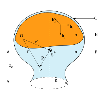
Figure 1: General variable mass system

The vector equation of attitude motion of such a system can be derived from the laws of mechanics (such as Newton-Euler equations, Lagrange’s method, etc.) and appropriately invoking Reynold’s Transport Theorem. This approach has been discussed in several papers [ekewang1 ; ekemao1 ; ekeme1 ]. The following is the equation of attitude motion of a general variable mass system

$${\bf M}^{*}= {\bf I}^{*}\cdot\textrm{\boldmath$\alpha$}+\textrm{\boldmath$\omega$}\times({\bf I}^{*}\cdot\textrm{\boldmath$\omega$})+\frac{{}^{B}d{\bf I}^{*}}{\mathrm{d}t}\cdot\textrm{\boldmath$\omega$}$$ (1)

$$+\int_{S_{0}}\rho\mathbf{[p\times(\textrm{\boldmath$\omega$}\times p)](v_{r}\cdot{n})}\,dS$$

$$+\int_{V_{0}}\rho\mathbf{[\textrm{\boldmath$\omega$}\times(p\times v_{r})]}\,dV+\frac{{}^{B}d}{\mathrm{d}t}\int_{V_{0}}\rho\mathbf{(p\times v_{r})}\,dV$$

$$+\int_{S_{0}}\rho\mathbf{(p\times v_{r})}(\mathbf{v_{r}}\cdot{\mathbf{n}})\,dS.$$

Several other forms of the equation of attitude motion have been derived for a variable mass system in the literature. However, Equation (1) is most tractable for examining the attitude evolution as it is decoupled from the translational dynamics. The volume integrals in Equation (1) are typically hard to evaluate in closed-form since the internal flow field is not generally known within a system. However, in the case of rockets, reasonable assumptions can be made about this internal flow. It is typically assumed that the internal flow of gases within a rocket relative to its casing is both steady and axisymmetric. Further assuming that the flow lacks a whirl component force the last three terms of Equation (1) to disappear, making it less cumbersome. Thus, the equation of attitude motion becomes

$${\bf M}^{*}={\bf I}^{*}\cdot\textrm{\boldmath$\alpha$} +\omega\times({\bf I^{*}}\cdot\textrm{\boldmath$\omega$})+\frac{{}^{B}d{\bf I}^{*}}{\mathrm{d}t}\cdot\textrm{\boldmath$\omega$}$$ (2)

$$+\int_{S_{0}}\rho\mathbf{\bigg{[}p\times(\textrm{\boldmath$\omega$}\times p)\bigg{]}(v_{r}\cdot{n})}\,dS.$$

The remainder of this paper concerns the torque-free motions of axisymmetric variable mass systems so $\mathbf{M^{*}=0}$. Note that though this non-whirling flow assumption is not realistic, it has been shown that the magnitude of the transverse angular rates are unaffected by such a flow assumption[ekewang3 ]. As stability information in this paper is derived from the magnitude of the angular rates, the non-whirling flow assumption is sufficient.

Referring back to Figure 1, ${\bf b}_{1},{\bf b}_{2},{\bf b}_{3}$ are a dextral set of unit vectors affixed in B and parallel to its principal directions. The instantaneous central inertia dyadic of this axisymmetric system is

$${\bf I}^{*}\triangleq I\,\,{\bf b}_{1}{\bf b}_{1}+I\,\,{\bf b}_{2}{\bf b}_{2}+J\,\,{\bf b}_{3}{\bf b}_{3}$$ (3)

where $I$ and $J$ are the instantaneous central principal moments of inertia of the variable mass system. Note that, the mass center, $S^{*}$ is not necessarily fixed relative to B and is always located on the symmetry axis, parallel to ${\bf b}_{3}$. Further, the inertial angular velocity of B at any instant is

$$\textrm{\boldmath$\omega$}\triangleq\omega_{1}{\bf b}_{1}+\omega_{2}{\bf b}_{2}+\omega_{3}{\bf b}_{3}$$ (4)

and, as a result, the inertial angular acceleration is

$$\textrm{\boldmath$\alpha$}=\dot{\omega}_{1}{\bf b}_{1}+\dot{\omega}_{2}{\bf b}_{2}+\dot{\omega}_{3}{\bf b}_{3}.$$ (5)

The first three terms on the right-hand side of Equation (2) evaluate to

$${\bf I}^{*}\cdot\textrm{\boldmath$\alpha$}=I\dot{\omega}_{1}{\bf b}_{1}+I\dot{\omega}_{2}{\bf b}_{2}+J\dot{\omega}_{3}{\bf b}_{3},$$ (6)

$$\textrm{\boldmath$\omega$}\times({\bf I}^{*}\cdot\textrm{\boldmath$\omega$})=\bigg{(}J-I\bigg{)}\omega_{2}\omega_{3}{\bf b}_{1}-\bigg{(}J-I\bigg{)}\omega_{1}\omega_{3}{\bf b}_{2},$$ (7)

and

$$\frac{{}^{B}d{\bf I}^{*}}{dt}\cdot\textrm{\boldmath$\omega$}=\dot{I}\omega_{1}{\bf b}_{1}+\dot{I}\omega_{2}{\bf b}_{2}+\dot{J}\omega_{3}{\bf b}_{3},$$ (8)

respectively. The assumed steady symmetry of the internal fluid flow is further constrained to be uniform along the exit plane so that ${\bf v_{r}\cdot n}=u={\text{c}onstant}$, which then yields the following expression for the surface integral in Equation (2)

$$\int_{S_{o}}\rho{\bf{p\times(\textrm{\boldmath$\omega$}\times p)(v_{r}\cdot{n})}}\,dS=$$ (9)

$$-\dot{m}\bigg{[}(z_{e}^{2}+\frac{R^{2}}{4})(\omega_{1}{\bf b_{1}}+\omega_{2}{\bf b_{2}}) +\frac{R^{2}}{2}\omega_{3}{\bf b_{3}}\bigg{]}.$$

where $\dot{m}$, the rate of mass loss, is given by

$$\dot{m}=-\rho_{exit}\pi R^{2}u=constant.$$ (10)

$\rho_{exit}$ is the assumed density of exhaust gases on the exit plane.

Substituting Equations (6), (7), (8), and (9) into Equation (2) yields

$$\dot{\omega}_{1}=\frac{I-J}{I}\omega_{2}\omega_{3}-\frac{1}{I}\bigg{[}\dot{I}-\dot{m}(z_{e}^{2}+\frac{R^{2}}{4})\bigg{]}\omega_{1}$$ (11)

$$\dot{\omega}_{2}=-\frac{I-J}{I}\omega_{3}\omega_{1}-\frac{1}{I}\bigg{[}\dot{I}-\dot{m}(z_{e}^{2}+\frac{R^{2}}{4})\bigg{]}\omega_{2}$$ (12)

and

$$\dot{\omega}_{3}=-\frac{1}{J}[\dot{J}-\dot{m}(\frac{R^{2}}{2})]\omega_{3}.$$ (13)

Equations (11)-(13) are the scalar equations of attitude motion for an axisymmetric, torque-free variable mass system with axisymmetric non-whirling internal mass flow. Equations (11) and (12) are commonly referred to as the equations of transverse motion while Equation (13) is the spin equation of motion; $\omega_{1}$ and $\omega_{2}$ are transverse rates and $\omega_{3}$ is the spin rate. The attitude motion of a variable system is characterized by solving these equations.

2.1 Spin rate

As the spin equation of motion is decoupled from the transverse equations of motion, an expression for the spin rate can be easily obtained and is given by

$$\omega_{3}=\omega_{30}\text{exp}(\Phi)$$ (14)

where

$$\Phi=-\int_{0}^{t}\bigg{[}\bigg{(}\dot{J}-\dot{m}R^{2}/2\bigg{)}/J\bigg{]}\mathrm{d}t.$$ (15)

If $J\triangleq mk_{3}^{2}$, where $k_{3}$ is the time-varying axial radius of gyration, then $\Phi$ evaluates to

$$\Phi=\int_{m(0)}^{m}\frac{(R^{2}/2)}{k_{3}^{2}}\frac{\mathrm{d}m}{m}+\mathrm{ln}\bigg{(}\frac{J(0)}{J}\bigg{)}.$$ (16)

Substituting for $\Phi$ in Equation (14) gives the following expression for the spin rate

$$\omega_{3}=\omega_{30}\frac{J(0)}{J}\text{exp}\bigg{(}\int_{m(0)}^{m}\frac{(R^{2}/2)}{k_{3}^{2}}\frac{\mathrm{d}m}{m}\bigg{)}$$ (17)

Examining Equation (17), the spin rate may decay, stay constant, grow, or fluctuate. Another observation that can be added to this is that the spin rate retains the polarity of its initial condition; if the initial condition is positive, then the spin rate is always non-negative, and vice versa. Further analysis in this chapter assumes a positive value for the initial spin rate. Additionally, if $k_{3}^{2}$ is assumed to be a constant in Equation (17), then

$$\omega_{3}=\omega_{30}\bigg{(}\frac{m(0)}{m}\bigg{)}^{1-\frac{R^{2}}{2k_{3}^{2}}}.$$ (18)

Equation (18) asserts that the spin rate can not fluctuate for a system with constant axial radius of gyration; it can only grow or decay monotonically, or stay constant. It can then also be inferred that a time-varying axial radius of gyration can lead to fluctuations in the spin rate. Thus, the radius of gyration has a crucial effect on the spin rate. These comments on the spin rate are in agreement with the work of Snyder and Warner [snyder ], and Wang and Eke [ekewang3 ].

2.2 Transverse rate

The transverse angular speeds can be solved for in a variety of different ways. Defining a complex variable $\omega_{c}$ as

$$\omega_{c}\triangleq\omega_{1}+j\omega_{2}$$ (19)

allows Equations (11) and (12) to be combined to yield a differential equation linear in $\omega_{c}$:

$$\dot{\omega}_{c}=\Bigg{\{}-j\frac{I-J}{I}\omega_{3}-\frac{1}{I}\bigg{[}\dot{I}-\dot{m}(z_{e}^{2}+\frac{R^{2}}{4})\bigg{]}\Bigg{\}}\omega_{c}.$$ (20)

Integrating Equation (20) yields

$${\omega}_{c}=\omega_{co}\cdot\Gamma\cdot\text{exp}\bigg{(}-j\chi\bigg{)}$$ (21)

where

$$\Gamma=\text{exp}\bigg{[}-\int_{0}^{t}\frac{1}{I}\bigg{[}\dot{I}-\dot{m}(z_{e}^{2}+\frac{R^{2}}{4})\bigg{]}\mathrm{d}t\bigg{]}$$ (22)

and

$$\chi=\int_{0}^{t}(1-\frac{J}{I})\omega_{3}\mathrm{d}t.$$ (23)

A consequence of Equation (23) is

$$\dot{\chi}=(1-\frac{J}{I})\omega_{3}$$ (24)

where $\dot{\chi}$ has the units of angular speed.

From Equations (21) and (19), the transverse speeds are given by

$$\omega_{1}=\Gamma(\omega_{10}\cos\chi+\omega_{20}\sin\chi)$$ (25)

$$\omega_{2}=\Gamma(-\omega_{10}\sin\chi+\omega_{20}\cos\chi)$$ (26)

and are oscillatory in nature.

Further, a transverse angular velocity vector $\omega$_t which lies in the plane made by the principal directions ${\bf b}_{1}$ and ${\bf b}_{2}$ can also be defined as

$$\textrm{\boldmath$\omega$}_{t}\triangleq\omega_{1}{\bf b}_{1}+\omega_{2}{\bf b}_{2},$$ (27)

whose magnitude is

$$\omega_{12}=||\textrm{\boldmath$\omega$}_{t}||=\sqrt{\omega_{1}^{2}+\omega_{2}^{2}}=\sqrt{\Gamma^{2}(\omega_{10}^{2}+\omega_{20}^{2})}=\Gamma\omega_{0}$$ (28)

where $\omega_{0}\triangleq\sqrt{\omega_{10}^{2}+\omega_{20}^{2}}=\text{constant}$. The principal directions may be chosen such that $\omega_{10}=0$ and $\omega_{20}=\omega_{0}$. This simplifies the appearance of the solutions in Equations (25) and (26) to

$$\omega_{1}=\omega_{0}\Gamma\sin\chi$$ (29)

$$\omega_{2}=\omega_{0}\Gamma\cos\chi.$$ (30)

Equation (27) can then be written as

$$\textrm{\boldmath$\omega$}_{t}=\omega_{0}\Gamma[\sin\chi{\bf b}_{1}+\cos\chi{\bf b}_{2}]=\omega_{0}\Gamma{\bf b}_{12}=\omega_{12}{\bf b}_{12},$$ (31)

where ${\bf b}_{12}=\sin\chi{\bf b}_{1}+\cos\chi{\bf b}_{2}$; ${\bf b}_{12}$ is clearly a unit vector that is orthogonal to ${\bf b}_{3}$. These developments concerning the transverse angular velocity vector will be useful in developments in Section 3 on the geometry of motion.

From examining Equations (31) and (22), it is evident that the spin rate has no influence on the magnitude of the transverse angular velocity. Further, it shows that the magnitude of the transverse angular velocity vector is a rescaling of $\omega_{0}$ by $\Gamma$, a function of time that can either grow, decay, or fluctuate. ${\bf b}_{12}$ is a unit vector that rotates in the plane of ${\bf b}_{1}$ and ${\bf b}_{2}$ at the angular speed $\dot{\chi}$. As revealed by Equation (24), $\dot{\chi}$ may be positive or negative (assuming that $\omega_{3}$ is always positive), depending on the relative values of $k_{1}$ and $k_{3}$; if $k_{3}>k_{1}$, then ${\bf b}_{12}$ rotates negatively in the body, advancing from ${\bf b}_{1}$ to $-{\bf b}_{2}$ and around; if $k_{1}>k_{3}$, then ${\bf b}_{12}$ rotates positively in the body, coinciding with ${\bf b}_{1}$ and then with ${\bf b}_{2}$ and so on. As the interest of this paper is in understanding the nutational stability, no attempt is made to obtain an analytically expression for $\chi$. Its value can be obtained numerically from Equation (23).

An expression for $\Gamma$ can be developed involving the system’s transverse radius of gyration, $k_{1}$. If $I\triangleq mk_{1}^{2}$, $\Gamma$ may be reformulated in Equation (22) as

$$\Gamma=\frac{I(0)}{I}\text{exp}\bigg{[}\int_{m(0)}^{m}\frac{\bigg{[}z_{e}^{2}+\frac{R^{2}}{4}\bigg{]}}{k_{1}^{2}}\frac{\mathrm{d}m}{m}\bigg{]}$$ (32)

Here, $R$ is the constant radius of the exit plane while $k_{1}$ and $z_{e}$ can vary; these are parameters that are modeling constraints. Substituting for $\Gamma$ into Equation (28) yields the following expression for the magnitude of the transverse angular velocity:

$$\omega_{12}=\omega_{0}\bigg{(}\frac{I(0)}{I}\bigg{)}\text{exp}\bigg{[}\int_{m(0)}^{m}\frac{\bigg{[}z_{e}^{2}+\frac{R^{2}}{4}\bigg{]}}{k_{1}^{2}}\frac{\mathrm{d}m}{m}\bigg{]}.$$ (33)

Some of the effects of the variations in $z_{e}$ and $k_{1}$ on the transverse rate will be studied in the subsequent passage on variable mass cylinders. However, it should be evident that $\omega_{12}$ can grow, decay, or fluctuate but under no circumstance is it constant for an axisymmetric variable mass system.

Finally, the inertial angular velocity of an axisymmetric variable mass system can now be written as

$$\textrm{\boldmath$\omega$}=\omega_{0}\Gamma{\bf b}_{12}+\omega_{3}{\bf b}_{3},$$ (34)

the form of which mimics the constant-mass rigid body case, for which $\Gamma=1$.

3 Geometry of Torque-free Motion and Nutation Angle Solution

Explicit description of the inertia parameters coupled with the developments regarding the angular speeds from the previous section are sufficient to visualize the motion of the angular velocity vector from the body-fixed frame. However, it is also possible to visualize its motion in an inertially fixed reference frame which is the focus of this section. These developments are then used to study the variable mass cylinder problem in the following section.

Exploiting the fact that the variable mass system’s angular momentum vector is fixed in inertial space [ekeme3 ; diss ] enables us to visually study the angular velocity evolution from an inertial frame. The angular momentum of a general variable mass system can be written as

$${\bf H}^{*}=\int_{V_{0}}\rho[{\bf p}\times[{\bf v}_{r}+(\textrm{\boldmath$\omega$}\times{\bf p})]\,\mathrm{d}V.$$ (35)

Retaining the assumption of steady and axisymmetric relative internal mass flow reduces Equation (35) to

$${\bf H}^{*}=\int_{V_{0}}\rho[{\bf p}\times(\textrm{\boldmath$\omega$}\times{\bf p})]\,\mathrm{d}V={\bf I}^{*}\cdot\textrm{\boldmath$\omega$}.$$ (36)

With the definitions of ${\bf I}^{*}$ and $\omega$ from Equations (3) and (4), respectively, the component form of the angular momentum vector is

$${\bf H}^{*}=I(\omega_{1}{\bf b}_{1}+\omega_{2}{\bf b}_{2})+J\omega_{3}{\bf b}_{3}$$ (37)

or

$${\bf H}^{*}=I\textrm{\boldmath$\omega$}_{t}+J\omega_{3}{\bf b}_{3}.$$ (38)

Using the component form of $\textrm{\boldmath$\omega$}_{t}$ from Equation (31) in Equation (38) gives

$${\bf H}^{*}=I\omega_{0}\Gamma{\bf b}_{12}+J\omega_{3}{\bf b}_{3}$$ (39)

Equation (39) gives an alternate form of the angular momentum of an axisymmetric variable mass system. Axisymmetric rigid systems (of constant or variable mass) are unique in that their angular momentum and angular velocity vectors are always in the same plane, evident by comparing Equations (34) to (39); ${\bf H}^{*}$ and $\omega$ are in the same plane formed by ${\bf b}_{12}$ and ${\bf b}_{3}$ and this is shown in Figure 2.

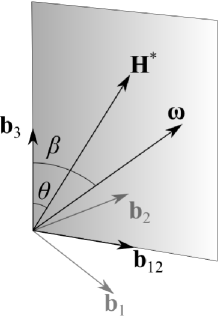
Figure 2: Geometry of motion setup of vectors

In this figure, $\theta$ is the angle between ${\bf H}^{*}$ and ${\bf b}_{3}$, and $\beta$ is the angle between ${\bf b}_{3}$ and $\omega$. These angles can be computed from the figure as

$$\theta=\tan^{-1}\bigg{(}\frac{I\omega_{12}}{J\omega_{3}}\bigg{)}=\tan^{-1}\bigg{(}\frac{\Gamma k_{1}^{2}\omega_{0}}{k_{3}^{2}\omega_{3}}\bigg{)}$$ (40)

and

$$\beta=\tan^{-1}\bigg{(}\frac{\omega_{12}}{\omega_{3}}\bigg{)}=\tan^{-1}\bigg{(}\frac{\Gamma\omega_{0}}{\omega_{3}}\bigg{)}.$$ (41)

Evaluation of these angles $\theta$ and $\beta$ along with the solutions to the angular velocities permit a visual understanding of the motion of the body in both inertial space and the body-fixed coordinate system.

In the case of axisymmetric rigid bodies of constant mass, $\Gamma=1$ and the spin rate and inertia scalars are constant. Consequently, in Equation (40) and (41), both angles evaluate to constants and visualizing the motion of $\omega$ results in the formation of two cones: as it rotates about ${\bf b}_{3}$ and another as it rotates about ${\bf n}_{h}$, a unit vector parallel to the inertially fixed ${\bf H}^{*}$. The two cones are appropriately named the body cone and space cone, respectively.

In the case of axisymmetric variable mass systems, angles $\theta$ and $\beta$ are typically functions of time. The angles may grow or decay as dictated by the instantaneous values of the radii of gyration, $\Gamma$, and the spin rate. It is also possible, in the case of the same variable mass system, for $\beta$ to exceed $\theta$ at certain instants while it may not at certain other instants. Figure 2 represents an instant where $\beta>\theta$, which occurs when $k_{3}>k_{1}$. Also, $\omega$ does not trace cones as it rotates about ${\bf b}_{3}$ and ${\bf n}_{h}$. Thus, generic names are used for the surfaces it traces; in this document, they are referred to as the body surface and space surface (which reduce to the ‘body cone’ and ‘space cone’ for the limiting case of a constant mass rigid body, respectively).

In the spacecraft dynamics literature, $\theta$ is referred to as the nutation angle [kaplan ]. In classical mechanics, $\theta$ may also be identified as the second Euler angle [likinstext ] and, thus, Equation (40) also gives the solution to said Euler angle. Growth in nutation angles results in a coning motion which is undesirable in spacecraft. Potential hazards of excessive nutation or coning motion might be poor initial conditions for subsequent mission operations, or possible loss of communications with a spacecraft due to incorrect pointing between its antenna and the base station. One such case of excessive nutation growth was observed in missions powered by the STAR-48 SRM [ekejpl ; meyer ; flandro ; cochran ; or ; mingori1 ; mingori2 ]. To mitigate this growth, an active nutation damper is used in these missions [webster ].

Closed form expressions to $\theta$ are available when the angular speeds are themselves available in closed form. These closed-form expressions are invaluable to not only evaluate stability but also for appropriate control strategy formulation to temper any instabilities. Solutions to the angular speeds are derived in the next section for a special class of variable mass systems: the axisymmetric variable mass cylinder. These closed form solutions are then utilized in constructing the body and space surfaces. The choice of cylindrical systems as an idealization is based on their use in several prior studies on rocket flight; Snyder and Warner [snyder ] and Eke et al. [ekewang2 ; ekemao2 ] are some examples of investigators who have incorporated cylindrical propellant grains in their studies on the attitude motions of variable mass space vehicles.

4 The Axisymmetric, Variable Mass Cylinder

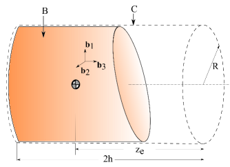
Figure 3: Variable mass cylinder

Figure 3 is that of a system that is initially a cylinder as represented by the dashed lines. The mass and inertia of this system is allowed to vary with time. As in the case of rockets, combustion is one plausible cause for these time-varying properties. Thus, at a general instant, some parts of the system may be solid while other parts are fluid. The solid part of the system is denoted $B$. The dotted line represents a control region $C$ of constant volume and surface area that has the same shape as the original cylinder and is rigidly attached to $B$. Only matter within $C$ at any instant is considered to make up the system. Interest here is in visualizing the motion of variable mass cylinders and understanding their nutational stability.

Equations (11)-(13) govern the attitude motion of the variable mass cylinder while Equations (17), (29), and (30) are the solutions to the angular speeds. Eke and Wang [ekewang2 ] identified idealized burn scenarios of which three are examined here. They are named the uniform burn, end burn, and radial burn. Each of these burns is explained in their respective sections. Inertia change due to fluid mass is neglected in all burn cases. The assumed properties of the system in creating the results presented are as follows. For the presented results, the density of the rigid propellant is assumed to be $1000$ kg/m³. The initial angular speeds are assumed to be $\omega_{0}=0.2$ rad/s, and $\omega_{30}=0.3$ rad/s; note that in a realistic rocket scenario, the spin rate would be an order of magnitude greater than the transverse rates. The duration of the burn is assumed to be $100$ s unless mentioned otherwise. Other assumptions concerning the geometry are discussed under each burn scenario.

4.1 Uniform Burn

A uniformly burning cylinder is one in which the mass of the system varies as a function of time while the dimensions of the unburned portion of the cylinder are the same as that of the original cylinder; radius and length of the cylinder are both assumed to be $1$m. Thus, its instantaneous central moment of inertia scalars are

$$I=m\bigg{(}\frac{R^{2}}{4}+\frac{h^{2}}{3}\bigg{)}$$ (42)

and

$$J=m\frac{R^{2}}{2}.$$ (43)

This is an example of a variable mass system where the radii of gyration are constant where $k_{1}^{2}=R^{2}/4+h^{2}/3$ and $k_{3}^{2}=R^{2}/4$. The time derivatives of the moment of inertia are

$$\dot{I} =\dot{m}(\frac{R^{2}}{4}+\frac{h^{2}}{3})$$ (44)

$$\dot{J} =\dot{m}\frac{R^{2}}{2}$$

The resulting spin and transverse rates are obtained from Equations (17) and (28) as

$$\omega_{3} = \omega_{30}$$ (45)

$$\omega_{12} = \omega_{0}\bigg{(}\frac{m}{m_{0}}\bigg{)}^{\frac{2h^{2}}{3k_{1}^{2}}}=\omega_{0}\Gamma(t)$$ (46)

where $\Gamma(t)\triangleq(m/m_{0})^{2h^{2}/3k_{1}^{2}}$. Prior to the start of the burn $m=m_{0}$ so $\Gamma=1$. As the burn proceeds $\Gamma$ decreases with time but is always non-negative. Thus, the transverse angular rate also decreases with time for a uniformly burning cylinder. Then Equation (40) gives the nutation angle for this system

$$\theta(t)=\tan^{-1}(K\Gamma(t)),$$ (47)

where $K=k_{1}^{2}\omega_{0}/k_{3}^{2}\omega_{30}$. Since $K$ is constant and $\Gamma(t)$ is decreasing with time, the nutation angle is also a decreasing parameter with time. This reduction in the transverse oscillations of a variable mass system by the exhaust gas is referred to as jet damping of a rocket.

The rotation of $\omega$ about ${\bf b}_{3}$ and ${\bf n}_{h}$ was discussed in the earlier section on generic axisymmetric variable mass systems. Figure 4 visualizes the first of these rotations for the uniformly burning cylinder, assuming $k_{3}>k_{1}$. The angular velocity vector traces a spiral in the transverse plane as it rotates about the symmetry axis ${\bf b}_{3}$ in a counter-clockwise direction and eventually converges to the symmetry axis.

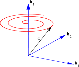
Figure 4: Uniform burn: body surface

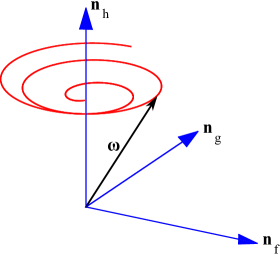
Figure 5: Uniform burn: space surface

The rotation of $\omega$ in the inertial space (i.e. about ${\bf n}_{h}$ since it is inertially fixed) requires knowledge of the angle, $\beta$, in Equation (41)

$$\beta=\tan^{-1}\bigg{(}\frac{\omega_{0}}{\omega_{30}}\bigg{(}\frac{m}{m(0)}\bigg{)}^{\frac{2h^{2}}{3k_{1}^{2}}}\bigg{)}.$$ (48)

This angle also decays with time for the uniformly burning cylinder, effectively reducing the system’s motion to that of simple or pure spin i.e. a motion in which the angular velocity and angular momentum vectors are parallel. The above expressions of $\theta$, and $\beta$ along with the angular velocity permit the construction of the space surface as shown in Figure 5. Note that ${\bf n}_{f}$, ${\bf n}_{g}$, and ${\bf n}_{h}$ represent a dextral set of unit vectors which are inertially fixed.

4.2 End Burn

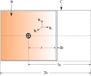
Figure 6: End burning cylinder

In this mechanism of mass variation, the cylinder burns from the circular face closest to the exit plane towards its other face. At any instant, the unburned part retains the shape of a right circular cylinder. Figure 6 represents a cylinder that burns from right to left. The axial radius of gyration for such a cylinder is constant, given by $k_{3}^{2}=R^{2}/4$. The corresponding axial moment of inertia is

$$J=mR^{2}/4\quad$$ (49)

As in the case of uniform burn, the spin rate can thus be determined from Equation (18) to be constant,

$$\omega_{3}=\omega_{30}.$$ (50)

The more interesting development occurs in the transverse directions. The transverse radius of gyration is $k_{1}^{2}=\frac{R^{2}}{4}+\frac{z^{2}}{3}$. Due to the changing length of the cylinder, $k_{1}$ is not a constant. Then, the transverse moment of inertia is

$$I=m(\frac{R^{2}}{4}+\frac{z^{2}}{3})$$ (51)

If $z$ is the instantaneous half length of the unburned cylinder, then its instantaneous mass is given by

$$m=\pi R^{2}(2z)$$ (52)

The rate of mass loss is then

$$\dot{m}=2\pi R^{2}\dot{z}.$$ (53)

which can also be written as

$$\mathrm{d}m=2\pi R^{2}\mathrm{d}z.$$ (54)

From Equations (52) and (54), it is possible to recast Equation (33) as

$$\omega_{12}=\omega_{0}\bigg{(}\frac{I(0)}{I}\bigg{)}\text{exp}\bigg{[}\int_{z_{0}}^{z}\frac{\bigg{[}z_{e}^{2}+\frac{R^{2}}{4}\bigg{]}}{\frac{R^{2}}{4}+\frac{z^{2}}{3}}\frac{\mathrm{d}z}{z}\bigg{]}.$$ (55)

Substituting $z_{e}=2h-z$ into Equation (55) gives

$$\omega_{12}=\omega_{0}\bigg{(}\frac{I(0)}{I}\bigg{)}\text{exp}\bigg{[}\int_{z_{0}}^{z}\frac{\bigg{[}z^{2}+4h^{2}-4hz+\frac{R^{2}}{4}\bigg{]}}{\frac{R^{2}}{4}+\frac{z^{2}}{3}}\frac{\mathrm{d}z}{z}\bigg{]}$$ (56)

which can also be reformulated as

$$\omega_{12}= \omega_{0}\bigg{(}\frac{I(0)}{I}\bigg{)}\text{exp}\bigg{[}\int_{z_{0}}^{z}\frac{3z-12h}{\frac{3R^{2}}{4}+z^{2}}\mathrm{d}z$$ (57)

$$+\bigg{(}12h^{2}+\frac{3R^{2}}{4}\bigg{)}\int_{z_{0}}^{z}\frac{\mathrm{d}z}{z\bigg{(}\frac{3R^{2}}{4}+z^{2}\bigg{)}}\bigg{]}.$$

A partial fraction expansion of the second integral in Equation (57) then gives

$$\omega_{12}= \omega_{0}\bigg{(}\frac{I(0)}{I}\bigg{)}\text{exp}\bigg{[}\int_{z_{0}}^{z}\frac{3z-12h}{\frac{3R^{2}}{4}+z^{2}}\mathrm{d}z$$ (58)

$$+\bigg{(}\frac{16h^{2}}{R^{2}}+1\bigg{)}\int_{z_{0}}^{z}\bigg{(}\frac{1}{z}-\frac{z}{\frac{3R^{2}}{4}+z^{2}}\bigg{)}\mathrm{d}z\bigg{]}$$

or, after some algebra,

$$\omega_{12}= \omega_{0}\bigg{(}\frac{I(0)}{I}\bigg{)}\text{exp}\bigg{[}-\int_{z_{0}}^{z}\frac{12h}{\frac{3R^{2}}{4}+z^{2}}\mathrm{d}z$$ (59)

$$-\bigg{(}\frac{16h^{2}}{R^{2}}-2\bigg{)}\int_{z_{0}}^{z}\frac{z}{\frac{3R^{2}}{4}+z^{2}}\mathrm{d}z$$

$$+\bigg{(}\frac{16h^{2}}{R^{2}}+1\bigg{)}\int_{z_{0}}^{z}\frac{\mathrm{d}z}{z}\bigg{]}.$$

The solution to the transverse rate is

$$\omega_{12}=\omega_{0}\bigg{(}\frac{I(0)}{I}\bigg{)}\text{exp}\bigg{[} \frac{8\sqrt{3}h}{R}\tan^{-1}\bigg{(}\frac{2\sqrt{3}R(z-h)}{3R^{2}+4zh}\bigg{)}$$ (60)

$$-\bigg{(}\frac{8h^{2}}{R^{2}}-1\bigg{)}\log\bigg{(}\frac{\frac{3R^{2}}{4}+z^{2}}{\frac{3R^{2}}{4}+h^{2}}\bigg{)}$$

$$+\bigg{(}\frac{16h^{2}}{R^{2}}+1\bigg{)}\log{\frac{z}{h}}\bigg{]}.$$

which can also be expressed as

$$\omega_{12}= \omega_{0}\bigg{(}\frac{I(0)}{I}\bigg{)}\bigg{(}\frac{\frac{3R^{2}}{4}+h^{2}}{\frac{3R^{2}}{4}+z^{2}}\bigg{)}^{\bigg{(}\frac{8h^{2}}{R^{2}}-1\bigg{)}}\bigg{(}\frac{z}{h}\bigg{)}^{\bigg{(}\frac{16h^{2}}{R^{2}}+1\bigg{)}}$$ (61)

$$\text{exp}\bigg{[}\frac{8\sqrt{3}h}{R}\tan^{-1}\bigg{(}\frac{2\sqrt{3}R(z-h)}{3R^{2}+4zh}\bigg{)}\bigg{]}.$$

The above solution can also be expressed in terms of the transverse radius of gyration as

$$\omega_{12}=\omega_{0} \bigg{(}\frac{k_{1}(0)}{k_{1}}\bigg{)}^{\frac{8h^{2}}{R^{2}}}\bigg{(}\frac{z}{h}\bigg{)}^{\frac{16h^{2}}{R^{2}}}$$ (62)

$$\text{exp}\bigg{[}\frac{8\sqrt{3}h}{R}\tan^{-1}\bigg{(}\frac{2\sqrt{3}R(z-h)}{3R^{2}+4zh}\bigg{)}\bigg{]}.$$

Equation (62) explains that, for an end burning cylinder, the transverse rate is regulated by 3 time varying functions: the ratio of the initial transverse radius of gyration to its instantaneous value, the ratio of the instantaneous half length to the initial half length, and an exponential function. The first of these functions grows as the burn progresses but is always bounded as its denominator is never zero. The latter two functions, however, always decay with time. Thus, irrespective of the nature of the cylinder, the transverse rates for the end burn are always decaying; the rate of decay is seen to be faster for prolate cylinders when compared to oblate cylinders, which makes sense in view of Equation (62). This has also been observed in Reference [ekewang2 ].

The nutation angle for an end-burning cylinder is given by

$$\theta(t)=\tan^{-1}(Kk_{1}^{2}\Gamma(t)),$$ (63)

where $K=\omega_{0}/k_{3}^{2}\omega_{30}=$ constant. As both $\Gamma(t)$ and $k_{1}$ are generally decreasing with time, the nutation angle decays with time for any end burning cylinder. In other words, jet damping is observed for such a mass-varying cylinder. Figures 7 and 8 show the body and space surfaces for end burning cylinders where the $J_{0}>I_{0}$ (initial $L$ = 1 m and $R$ = 0.8 m) whereas Figures 9 and 10 are for end-burning cylinders where $J_{0}<I_{0}$ (initial $L$ = 1 m and $R$ = 0.5 m). It is interesting to note in the second case (where $J_{0}<I_{0}$) that the angular velocity vector changes its direction of rotation, about both ${\bf b}_{3}$ and ${\bf n}_{h}$. Initially, it rotates in a clockwise direction and then switches to a counterclockwise direction, eventually converging to a pure spin about ${\bf b}_{3}$ in the body frame and ${\bf n}_{h}$ in the inertial frame. This transition point occurs when the ratio of the axial radius of gyration to the transverse radius of gyration falls below 1 and changes the sign of $\dot{\chi}$ as given by Equation (24). In either case, the end burn is seen to exhibit a decay in the cone angle and is thus nutationally stable.

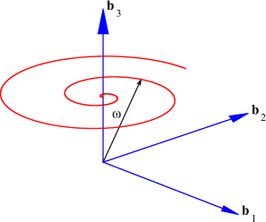
Figure 7: End burn: body surface ($J_{0}>I_{0}$)

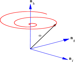
Figure 8: End burn: space surface ($J_{0}>I_{0}$)

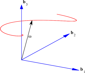
Figure 9: End burn: body surface ($J_{0}<I_{0}$)

H

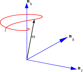
Figure 10: End burn: space surface ($J_{0}<I_{0}$)

4.3 Radial burn

In radial burn, combustion starts along the symmetry axis and proceeds radially outwards. Thus, at any instant, the unburned portion resembles a hollow pipe and both the axial and transverse radius of gyration of the system are variable as shown in Figure 11.

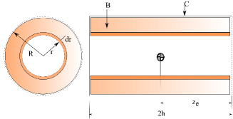
Figure 11: Radially burning cylinder

For the results presented here, initial radius and length are $1$ m. The instantaneous moment of inertia scalars for the radially burning cylinder are

$$I=m(\frac{R^{2}+r^{2}}{4}+\frac{h^{2}}{3})$$ (64)

and

$$J=m\frac{R^{2}+r^{2}}{2}.$$ (65)

Their corresponding time derivatives are

$$\dot{I} =\dot{m}(\frac{R^{2}}{2}+\frac{h^{2}}{3})$$ (66)

$$\dot{J} =\dot{m}{r^{2}}.$$

The angular speeds evaluate to

$$\omega_{3}=\omega_{30}\frac{R^{4}}{(R^{2}+r^{2})\sqrt{(R^{2}+r^{2})(R^{2}-r^{2})}}$$ (67)

$$\omega_{12}=\omega_{0}\bigg{(}\frac{R^{2}+{4h^{2}}/3}{R^{2}+{4h^{2}/3+r^{2}}}\bigg{)}^{\frac{(3R^{2}+16h^{2}/3)}{(2R^{2}+4h^{2}/3)}}\bigg{(}\frac{R^{2}-r^{2}}{R^{2}}\bigg{)}^{\frac{(-R^{2}+8h^{2}/3)}{(2R^{2}+4h^{2}/3)}}.$$ (68)

Evidently, the spin rate is not constant for a cylinder subject to radial burn. It varies such that it appears to damp out, slowly, for about two-thirds of the burn. Towards the end of the burn, i.e. as $r$ approaches $R$, the spin rate grows without bounds. Analytically, this growth in spin rate has been found to begin at the instant $r/R=0.707$ [ekemao3 ]. The transverse angular speed, on the other hand, can either grow, decay, or fluctuate depending on the shape of the cylinder before the start of the burn. The corresponding body and space surfaces for the radially burning cylinder are shown in Figures 12 and 13, respectively, for a burn duration of $90$ s; this duration is chosen purely to study a case where the end mass of the system approaches the mass of a payload.

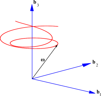
Figure 12: Radial burn: body surface

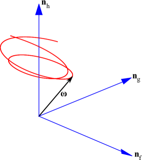
Figure 13: Radial burn: space surface

The case presented here is for $R/h=2$ and is a nutationally stable configuration; this is in agreement with Mao and Eke’s work [ekemao3 ] where it was shown that transverse rates are unbounded for oblate radially burning cylinders with a $R/h\geq\sqrt{8/3}$. The cone angle does in fact monotonically decrease though this is not as evident from Figure 12 when compared to the uniform and end burns; this is primarily due to the fact that the system’s end mass is approximately 315 kg at the end of this radial burn whereas in the other burns it is nearly zero. One approach to verifying the nutational stability of the system is by plotting the time evolution of $\theta$. However, the stability can also be verified from the angular speeds. For the extreme case of oblateness represented by a radially burning flat disk (i.e. $R>>h$), Equation (68) can be reformulated as

$$\omega_{12}=\omega_{0}\frac{\omega_{3}}{\omega_{30}}$$ (69)

by dropping the terms involving $h$ from the solution to the transverse speed. Extending this rationale to the inertia scalars given by Equation (64) and (65), we also get $I/J=1/2$. Then, the nutation angle from Equation (40) can be expressed as

$$\theta=\tan^{-1}\bigg{(}\frac{\omega_{0}}{2\omega_{30}}\bigg{)}=\text{constant}.$$ (70)

which is clearly bounded. In other words, even the most oblate configuration of a radially burning cylinder results in a constant nutation angle and thus does not show growth in the coning motion. However, unlike the preceding burns, the radial burn would require a nutation damper system to attenuate the cone angle and bring the system into a state of pure spin.

5 Conclusion

A graphical approach to study the coning motion, also known as the geometry of motion, of a torque-free, axisymmetric variable mass system is developed. Based on this, a general solution to the second Euler angle is also presented. The theoretical development is seen to augment well with the work on constant mass rigid bodies. Following these developments, the coning motion is specifically explored for an axisymmetric cylinder with mass loss subject to three idealized burns: the uniform, end, and radial burns. The uniform and end burning cylindrical configurations exhibit constant spin rates and bounded decaying transverse rates; they are seen to be nutationally stable. The radial burn generally exhibits unbounded spin rates whereas the transverse rate is unbounded only for more oblate configurations. More interestingly, even these oblate configurations are seen to show stable coning motion. In relation to rocket dynamics, the results presented here show that oblate configurations that exhibit a “misbehavior” in their transverse rates could still be nutationally stable. The difference between the radial burn from the other burns examined is that the system does not always approach a state of pure spin. This work recommends that examining the transverse speed alone may be insufficient in determining the stability of a freely rotating variable mass system.

The rotational behavior of a free axisymmetric variable mass system is remarkably different from its constant mass counterpart. For a free axisymmetric system with mass variation, spin rates are functions of time that either grow, decay, or remain constant whereas their transverse speeds can either grow or decay; on the other hand, the spin and transverse speeds of constant mass systems are of constant magnitude. As the inertia properties in the latter case are also constant, the corresponding nutation angle (or second Euler angle) is also unchanging which leads to the well known ‘cones of motion’ of the angular velocity. In the case of variable mass systems, the nutation angle is not as straightforward to generally characterize on account of the time-varying nature of both the angular velocity and its central inertia scalars. Thus, the results of the analyses presented clearly indicate that mass variation majorly impacts the dynamics of freely spinning systems.

Compliance with ethical standards

Conflict of interest The authors declare that they have no conflict of interest.

References

- (1) Barkley Rosser J., Newton, R.R., Gross, G.L.: Mathematical Theory Of Rocket Flight. McGraw-Hill, New York, (1947)
- (2) Reiter, G., Thomson, W.: Jet damping of a solid rocket-theory and flight results. AIAA J., 3, 413–417 (1965)
- (3) Thomson, W.T.: Equations of motion for the variable mass system. AIAA J., 4, 766–768 (1966)
- (4) Thomson, W. T., Introduction to Space Dynamics, New York: Dover (1986)
- (5) Eke, F.O., Wang, S.-M.: Equations of motion of two-phase variable mass systems with solid base. J. Appl. Mech., 61(4), 855-860 doi:10.1115/1.2901568 (1994)
- (6) Eke, F.O., Mao, T.C.: On the dynamics of variable mass systems, International J. Mech. Eng. Educ., 30(2), 123-137 doi:10.7227/IJMEE.30.2.4 (2002)
- (7) Nanjangud, A., Eke, F.O.: Lagrange’s equations for rocket-type variable mass systems, International Rev. Aerosp. Eng., 5(5), 256-260 (2012)
- (8) Djerassi, S.: Algorithm for simulation of motions of variable-mass systems. J. Guid. Control Dyn., 21, 427–434 (1998)
- (9) Banerjee, A.K.: Dynamics of a variable-mass, flexible-body system. J. Guid. Control Dyn., 23, 501-508 (2000)
- (10) Hu, P., Ren, G.: Multibody dynamics of flexible liquid rockets with depleting propellant. J. Guid. Control, and Dyn., 36, 1840–1849 (2013)
- (11) Cveticanin, L., Djukic, Dj.: Motion of body with discontinual mass variation. Nonlinear Dyn. 52(3), 249-261, (2008). doi:10.1007/s11071-007-9275-5 (2007)
- (12) Cveticanin, L.: Dynamics of body separation—analytical procedure. Nonlinear Dyn. 55(3), 269-278 (2007)
- (13) Eke, F.O., Wang, S.-M.: Attitude behavior of a variable mass cylinder. J. Appl. Mech., 62(4), 935-940 (1995)
- (14) Wang, S.-M., Eke, F.O., Rotational dynamics of axisymmetric variable mass systems. J. Appl. Mech., 62(4), 970-974 (1995)
- (15) Eke, F.O., Mao, T.-C., Morris, M. J., Free attitude motions of a spinning body With substantial mass loss. J. Appl. Mech., 71(2), 190-194 (2004)
- (16) Eke, F.O., Star 48 Coning Anomaly. JPL Internal Document, 989 (1982)
- (17) Flandro, G.A., Van Moorhem, W.K., Shorthill, R., Chen, K., Woolsey, M.: Fluid mechanics of spinning rockets. U.S. Air Force Rocket Propulsion Lab. Rept. TR-86-072, Edwards AFB, CA, Jan. 1987
- (18) Ha, J.C.V.D., Janssens, F.L.: Jet-damping and misalignment effects during solid rocket motor burn. J. Guid. Control Dyn., 28, 412–420 (2005)
- (19) Nanjangud, A., Eke, F.O.: Approximate solution to the angular speeds of a nearly-symmetric mass-varying cylindrical body. The J. Astronautical Sci., 64(2), 99-117 (2017)
- (20) Likins, P.W., Elements of Engineering Mechanics. McGraw-Hill, New York (1973)
- (21) Kaplan, M.H., Modern Spacecraft Dynamics and Control. Wiley, New York (1976)
- (22) Ayoubi, M.A., Martin, K.M., Longuski, J.M.: Analytical solution for spinning thrusting spacecraft with transverse ramp-up torques. J. Guid. Control Dyn., 37(4), 1272-1282 (2014)
- (23) Martin, K.M., Longuski, J.M.: Velocity pointing error reduction for spinning, thrusting spacecraft via heuristic thrust profiles. J. Spacecr. Rockets, 52(4), 1268-1272 (2015)
- (24) Javorsek,D., Longuski,J. M.: Velocity pointing errors associated with spinning thrusting spacecraft. J. Spacecr.Rockets,37(3), 359–365 (2000)
- (25) Nanjangud, A., Eke, F.O.:Angular momentum of free variable mass systems is partially conserved, Aerosp. Sci. Tech., doi:10.1016/j.ast.2018.03.003 (2018)
- (26) Nanjangud, A.: On the rotational dynamics of variable mass systems. PhD dissertation, University of California, Davis (2016)
- (27) Mao, T.C., Eke, F.O., Attitude dynamics of a torque-free variable mass cylindrical body. J. Astronaut. Sci., 48, 435-448 (2000)
- (28) Meyer, R. X.: Convective instability in solid propellant rocket motors. Adv. Astronaut. Sci., 54, 173 (AAS Paper 83-368) (1983)
- (29) Cochran, J.E., Jr., Kang, J.Y.: Nonlinear stability analysis of the attitude motion of a spin-stabilized upper stage. Adv. Astronaut. Sci., 75(1), 345–364 (1991)
- (30) Or, A.C.: Rotor-pendulum model for the perigee assist module nutation anomaly. J. Guid. Control Dyn., 15(2), 297-303, (1992).
- (31) Mingori, D., Yam, Y.: Nutational stability of a spinning spacecraft with internal mass motion and axial thrust. AIAA Paper 86-2271 AIAA Astrodynamics Conference Proceedings (Williamsburg, VA), 367-375, AIAA, Washington, DC (1986)
- (32) Halsmer, D.M., Mingori, D.L: Nutational stability and passive control of spinning rockets with internal mass motion. J. Guid. Control Dyn., 18(5), 1197-1203 (1995)
- (33) Webster, E.: Active nutation control for spinning solid motor upper stages. American Institute of Aeronautics and Astronautics (1985)
- (34) Snyder, V.W., and Warner, G.G., A re-evaluation of jet damping. J. Spacecr. Rockets, 5, 364-366 (1968)