Higher-order QCD corrections to hadronic $\tau$ decays from Padé approximants

Abstract

Perturbative QCD corrections to hadronic $\tau$ decays and $e^{+}e^{-}$ annihilation into hadrons below charm are obtained from the Adler function, which at present is known in the chiral limit to five-loop accuracy. Extractions of the strong coupling, $\alpha_{s}$, from these processes suffer from an ambiguity related to the treatment of unknown higher orders in the perturbative series. In this work, we exploit the method of Padé approximants and its convergence theorems to extract information about higher-order corrections to the Adler function in a systematic way. First, the method is tested in the large-$\beta_{0}$ limit of QCD, where the perturbative series is known to all orders. We devise strategies to accelerate the convergence of the method employing renormalization scheme variations and the so-called D-log Padé approximants. The success of these strategies can be understood in terms of the analytic structure of the series in the Borel plane. We then apply the method to full QCD and obtain reliable model-independent predictions for the higher-order coefficients of the Adler function. For the six-, seven-, and eight-loop coefficients we find $c_{5,1}=277\pm 51$, $c_{6,1}=3460\pm 690$, and $c_{7,1}=(2.02\pm 0.72)\times 10^{4}$, respectively, with errors to be understood as lower and upper bounds. Our model-independent reconstruction of the perturbative QCD corrections to the $\tau$ hadronic width strongly favours the use of fixed-order perturbation theory (FOPT) for the renormalization-scale setting.

1 Introduction

The precise determination of the strong coupling, $\alpha_{s}$, is a key ingredient for calculations of all processes involving perturbative Quantum Chromodynamics (QCD) and represents a fundamental test of the internal consistency of the Standard Model. The value of $\alpha_{s}$, together with the mass of the top quark, plays, for example, a crucial role in the fate of the Standard Model vacuum [1]. The extraction of $\alpha_{s}$ from hadronic $\tau$ decays [2, 3, 4, 5] (and also from $e^{+}e^{-}\to(\mbox{hadrons})$ below charm [6, 7]) is of special interest for two reasons. First, because it is done at relatively low energies, close to the limit of validity of perturbative QCD. Therefore, the evolution of $\alpha_{s}$ from the $\tau$ mass scale to the $Z$ mass scale represents one of the most non-trivial tests of asymptotic freedom [8] as predicted by the QCD $\beta$-function [9, 10, 11, 12]. Second, this determination of $\alpha_{s}(m_{Z})$ is competitive, since the running reduces the size of the relative error.

However, theoretical uncertainties still affect the determination of $\alpha_{s}$ from these processes. At and around the $\tau$ mass, perturbative QCD is still valid, but non-perturbative effects become non-negligible. These effects are smaller by a factor of about ten when compared to the perturbative QCD contribution, but must be taken into account carefully [3, 13]. They are encoded in the condensates of the Operator Product Expansion (OPE) and the related contributions from violations of quark-hadron duality — or simply duality violations (DVs) [14, 15, 16, 17].

Another important source of uncertainty stems from the renormalization-scale setting in the perturbative contribution. Theoretically, the decay $\tau\to({\rm hadrons})+\nu_{\tau}$ is expressed in terms of a weighted integral of the hadronic spectral functions that runs over the hadronic invariant mass squared from threshold up to $m_{\tau}^{2}$. Since perturbative QCD cannot be trusted at low energies, one resorts to Finite Energy Sum Rules (FESRs) to relate this integral to an integral along a closed contour in the complex plane with $|s|=m_{\tau}^{2}$. In this process, a procedure must be adopted to set the renormalization scale. The two most commonly employed procedures are known as Fixed Order Perturbation Theory (FOPT) [18] and Contour Improved Perturbation Theory (CIPT) [19, 20] (they are discussed in more detail below). The two represent different ways of treating the unknown higher orders in perturbation theory, and lead to different perturbative series and, therefore, to different values of $\alpha_{s}$. This remains true in the analogous extraction of $\alpha_{s}$ from $e^{+}e^{-}\to(\mbox{hadrons})$ below charm although, numerically, the difference between the two procedures is smaller in that case [7].

The elimination of this ambiguity is inherently difficult because it requires knowledge about higher orders of the perturbative expansion. At present, the perturbative QCD expansion of the Adler function in the chiral limit is known up to $\alpha_{s}^{4}$ thanks to the five-loop computation of Ref. [21, 22] and it is unlikely that the result at six loops will be available anytime soon [23]. In the absence of exact calculations for the higher-order coefficients, one must tackle this problem with methods that allow for a partial reconstruction of the series based only on the available information.

The general structure of the perturbative series is assumed to be known. It is an asymptotic series (therefore divergent) with coefficients that grow factorially. The divergent behaviour of the series is governed by renormalons: singularities along the real axis of the Borel transformed series [24]. The position of these singularities is known since they are related to the dimension of operators that participate in the OPE of the relevant correlator. The exponents of the singularities are related to the anomalous dimension of the same operators and can, in principle, be calculated. On the other hand, nothing, essentially, is known about the residues of the singularities.

This partial knowledge has been used to construct realistic representations of the full series by approximating its Borel transform, which has an infinite tower of singularities, by a small number of dominant ones [18, 25]. These models for the Borel transformed series are, in some cases, a type of rational or Padé approximant. Motivated by this observation, in this paper we investigate, systematically, the use of Padé theory [26, 27, 28, 29] to reconstruct the Adler function, which governs hadronic $\tau$ decays and the cross section of $e^{+}e^{-}\to(\mbox{hadrons})$. One of the main advantages of the use of rational approximants, as compared to the so-called renormalon models of Refs. [18, 25], is that they can be made model independent. Additionally, in some well defined cases, theorems guarantee the convergence of a sequence of approximants to the function of interest.

In the past, rational approximants have already been used in the context of $\tau$ decays [30]. In particular, the observation that their convergence can be improved when one uses the Borel transformed series, as opposed to the series in $\alpha_{s}$, was already made. (This procedure is sometimes referred to as “Padé-Borel method” [31].) At that time, however, the perturbative series was known to one order less, only up to $\alpha_{s}^{3}$. Moreover, the connection with renormalons in applications to $\tau$ decays was not made explicitly. Here, this connection is established and we are able to use different types of Padé approximants (such as partial Padé approximants) thanks to the available knowledge about the renormalon singularities.

To validate our approach, before applying Padé approximants (PAs) to full QCD, we will work within the large-$\beta_{0}$ limit. In this limit, one obtains all the corrections with highest power of $N_{f}$ at every given $\alpha_{s}$ order in the perturbative expansion (with $N_{f}$ being the number of light-quark flavours). The application of this procedure to $\tau$ decays generates an asymptotic series in $\alpha_{s}$ that is known to all orders, and the result for the Borel transformed Adler functionn can be written in a compact form [33, 34]. This Borel transform is a meromorphic function in the complex plane: it has a finite radius of convergence and an infinite number of renormalon poles along the real axis, but no branch cut. Therefore, the theory of PAs to meromorphic functions, and in particular Pommerenke’s theorem, apply [26, 35]. Apart from the standard PAs, we will consider several strategies for accelerating the convergence of the approximation. First, we will exploit the renormalization scheme dependence of the perturbative series, following Ref. [36], to optimize the convergence of the Padé approximants to exactly known Adler function. Additionally, we will consider partial Padé approximants (which exploit the available knowledge about the renormalon singularities). We will also employ D-log Padé approximants [26] which can also be very effective in approximating functions with branch cuts. Finally, we investigate the application of the different PAs to the FOPT expansion of the QCD corrections to the $\tau$ hadronic width. This series has a much simpler analytic structure in the Borel plane, which leads to coefficients that follow a more regular pattern, and is more amenable to approximation by rational functions. From these approximants one can easily perform an indirect reconstruction of the Adler function that is very reliable and requires little information.

The systematic study performed in large-$\beta_{0}$ and the lessons we learn from this limit are used as the basis for the QCD analysis. In the case of full QCD, the structure of the Borel transformed Adler function is more involved, since the poles become branch cuts [24]. From renormalization scheme variations we find indications that in QCD the leading UV renormalon is suppressed with respect to large-$\beta_{0}$ and, as a consequence, the sign alternation of the series is probably postponed. We will then show that, as in large-$\beta_{0}$, it is advantageous to consider Padé approximants to the FOPT expansion of the corrections to the $\tau$ hadronic width. From these approximants, we are able to obtain reliable model-independent predictions for the higher-order coefficients of the Adler function, together with an estimate of their uncertainty, and extract an estimate for the ressumed value of the perturbative QCD corrections to hadronic $\tau$ decays. We are also in a position to discuss the renormalization group improvement of the series and we show, from our reconstruction of high orders, that FOPT is strongly favoured in QCD. The systematic use of PAs lead to results that are model independent and that have significantly smaller errors than results obtained from other methods.

Our work is organized as follows. In Sec. 2 we describe the essentials about the QCD description of hadronic $\tau$ decays and, in Sec. 3, we collect the main facts about Padé theory relevant to this work. Then, in Sec. 4, we apply the Padé approximants to the large-$\beta_{0}$ limit of QCD. The results in full QCD are presented in Sec. 5 and the conclusions are given in Sec. 6.

2 Perturbative QCD in hadronic $\tau$ decays

In the study of perturbative QCD corrections to hadronic $\tau$ decays and $e^{+}e^{-}\to(\mbox{hadrons})$ below charm the central object is the Adler function in the chiral limit (defined below). From the knowledge of its expansion one can derive the corrections to the $\tau$ hadronic width [18] as well as the perturbative expansion of $R(s)$ for $e^{+}e^{-}\to(\mbox{hadrons})$ below charm [7]. In the spirit of being self-contained, we review here the main aspects of the theoretical description of hadronic $\tau$ decays in QCD. (We refer to Refs. [2, 18, 40] for further details.) Although we frame our discussion in the context of $\tau$ decays the application to $e^{+}e^{-}\to(\mbox{hadrons})$ is straightforward and is, essentially, a matter of normalization to reflect the fact that the current in that case is the electromagnetic one. For the details regarding this normalization we refer to Ref. [7].

The decay rate of $\tau\to({\rm hadrons})+\nu_{\tau}$ can be separated experimentally into three components: a vector and an axial-vector, due to decays mediated by the light-quark $\bar{u}d$ current, and strange contributions, arising from the $\bar{u}s$ current. These decay rates, normalized to the width of $\tau\to e\bar{\nu}_{e}\nu_{\tau}$, are denoted $R_{\tau,V}$, $R_{\tau,A}$, and $R_{\tau,S}$, respectively. When extracting $\alpha_{s}$ it is convenient to work only with light quarks, because corrections proportional to the mass of the quarks can then be safely neglected. Here, we restrict ourselves to the non-strange channels, precisely for this reason. Then, the different corrections to the partonic result can be parametrized as

$$R_{\tau,V/A}=\frac{N_{c}}{2}S_{\rm EW}|V_{ud}|^{2}\left[1+\delta^{(0)}+\delta_{\rm NP}+\delta_{\rm EW}\right],$$ (1)

where $S_{\rm EW}$ and $\delta_{\rm EW}$ are small electroweak corrections and $V_{ud}$ the CKM matrix element; the unity, in between square brackets, is simply the partonic result. The first correction, $\delta^{(0)}$, is the perturbative QCD part, which is the dominant contribution ($\sim 20\%$). Non-perturbative contributions, encoded in $\delta_{\rm NP}$, are significantly smaller and contain both OPE condensates and DVs. In this work, we focus on the perturbative QCD part, $\delta^{(0)}$, that we discuss in more detail below.

The relevant quantity that governs $R_{\tau,V/A}$ are the correlators

$$\Pi_{V/A}^{\mu\nu}(p)\equiv i\int dx\,e^{ipx}\,\langle\Omega|T\{J_{V/A}^{\mu}(x)J_{V/A}^{\nu}(0)^{\dagger}\}|\Omega\rangle,$$ (2)

where $\left|\Omega\right\rangle$ represents the physical vacuum and the currents are $J^{\mu}_{V/(A)}(x)=(\bar{u}\gamma^{\mu}(\gamma_{5})d)(x)$. These correlators can be decomposed into transverse, $\Pi^{(1)}_{V/A}(s)$, and longitudinal, $\Pi^{(0)}_{V/A}(s)$, parts in the usual way (with $s=p^{2}$). The decay rate can be expressed in terms of integrals over the spectral functions, $\frac{1}{\pi}{\rm Im}\Pi^{J}_{V/A}(s)$, that run from $s=0$ to $s=m_{\tau}^{2}$ [2, 18]. These integrals, on the theory side, are problematic because perturbative QCD is not valid at low energies. To circumvent this problem, one resorts to a FESR that exploits the analyticity properties of the correlators. The quantities $R_{\tau,V/A}$ can then be expressed as an integral in a closed contour in the complex plane with fixed $|s|=m_{\tau}^{2}$. Explicitly, for the perturbative contribution, one finds [18]

$$\delta^{(0)}=\frac{1}{2\pi i}\oint\displaylimits_{|x|=1}\frac{dx}{x}W(x)\widehat{D}^{(1+0)}_{\rm pert}(m_{\tau}^{2}x),$$ (3)

with $x=s/m_{\tau}^{2}$ and where the weight function $W(x)$, determined by phase space, is $W(x)=(1-x)^{3}(1+x)$. In this integral, $\widehat{D}^{(1+0)}_{\rm pert}$ is the perturbative contribution to the reduced Adler function defined as

$$1+\widehat{D}_{\rm pert}(Q^{2})=\frac{12\pi^{2}}{N_{c}}D^{(1+0)}_{\rm pert}(Q^{2}),$$ (4)

where the Adler function itself, $D^{(1+0)}$, is obtained as the logarithmic derivative of the combination $\Pi^{(1+0)}(s)$ as

$$D^{(1+0)}(s)=-s\frac{d}{ds}\left[\Pi^{(1+0)}(s)\right].$$ (5)

The Adler function is a physical object in the sense that it does not contain subtraction constants that depend on the renormalization conventions. This function is central to our work.

The perturbative expansion of $\widehat{D}$ starts at $\mathcal{O}(\alpha_{s})$ and can be cast as

$$\widehat{D}_{\rm pert}(s)=\sum\limits_{n=1}^{\infty}{a^{n}_{\mu}}\sum\limits_{k=1}^{n+1}{kc_{n,k}L^{k-1}},$$ (6)

where $L=\log(-s/\mu^{2})$ and $a_{\mu}=\alpha_{s}(\mu)/\pi$. In this expansion, the only independent coefficients are the $c_{n,1}$; the others can be obtained imposing renormalization group (RG) invariance, and are expressed in terms of the $c_{n,1}$ and $\beta$-function coefficients [18, 41]. The logarithms can be summed with the scale choice $\mu^{2}=-s\equiv Q^{2}$ giving

$$\widehat{D}_{\rm pert}(Q^{2})=\sum\limits_{n=1}^{\infty}{c_{n,1}a^{n}_{Q}}\equiv\sum_{n=0}^{\infty}r_{n}\alpha_{s}^{n+1}(Q).$$ (7)

where $r_{n}=c_{n+1,1}/\pi^{n+1}$. With this definition, the perturbative expansion of the reduced Adler function with the choice $\mu^{2}=Q^{2}$ then reads (for $N_{f}=3$, ${\overline{\rm MS}}$ scheme)

$$\widehat{D}(Q^{2})=a_{Q}+1.640\,a_{Q}^{2}+6.371\,a_{Q}^{3}+49.08\,a_{Q}^{4}+\cdots,$$ (8)

from which the numerical values of the known independent coefficients $c_{n,1}$ of Eq. (7) can be immediately read off.

The perturbative series of Eq. (6) is divergent and one assumes that it must be an asymptotic expansion to the true value of the function being expanded [24]. To study the perturbative contribution to the Adler function, and in particular its renormalon content, it is therefore convenient to work with the Borel transformed series, which can have a finite radius of convergence, defined as

$$B[\widehat{D}](t)\equiv\sum\limits_{n=0}^{\infty}{r_{n}\frac{t^{n}}{n!}}.$$ (9)

The original expansion, in turn, can be understood as an asymptotic series to the inverse Borel transform

$$\widehat{D}(\alpha)\equiv\int\limits_{0}^{\infty}{dt\text{e}^{-t/\alpha}B[\widehat{D}](t)},$$ (10)

provided that the integral exists. The last equation defines the Borel sum of the asymptotic series. The divergence of the original series, $\widehat{D}$, is translated into singularities in the $t$ variable. Two types can be distinguished: ultraviolet (UV) and infrared (IR) renormalons. The UV renormalons lie on the negative real axis and contribute with sign alternating coefficients. IR renormalons are singularities on the positive real axis which contribute with fixed sign coefficients. The latter obstruct the integration in Eq. (10) and generate an ambiguity in the inverse Borel transform which is expected to cancel against power corrections of the OPE. The position of the singularities in the $t$ plane can be determined with general renormalization group (RG) arguments. They appear at positive and negative integer values of the variable $u\equiv\frac{\beta_{1}t}{2\pi}$ (except for $u=1$), where $\beta_{1}$ is the leading coefficient of the QCD $\beta$-function. The UV renormalon at $u=-1$, being the closest to the origin, dominates the large order behaviour of the series, which must, therefore, be sign alternating at higher orders. As seen in Eq. (8), this sign alternation is still not apparent in the first four coefficients of the QCD expansion in the ${\overline{\rm MS}}$ scheme, which are known exactly.

Finally, to obtain the perturbative corrections to $R_{\tau,{V/A}}$ one needs to perform the integral in Eq. (3). In the process, one needs to adopt a procedure in order to set the scale $\mu$, which enters, implicitly, through Eq. (6). A running scale, $\mu^{2}=Q^{2}$, as done in Eq. (7), gives rise to the aforementioned Contour-Improved Perturbation Theory (CIPT), where the running of $\alpha_{s}$ along the contour is resummed to all orders. In this case, $\delta^{(0)}$ can be written as

$$\delta^{(0)}_{\rm CI}=\sum_{n=1}^{\infty}c_{n,1}J_{n}^{\rm CI}(m_{\tau}^{2}),\qquad\mbox{with}\qquad J_{n}^{\rm CI}=\frac{1}{2\pi i}\oint\displaylimits_{|x|=1}\frac{dx}{x}(1-x)^{3}(1+x)a^{n}(-m_{\tau}^{2}x).$$ (11)

Another option is to employ a fixed scale $\mu^{2}=m_{\tau}^{2}$, which gives rise to Fixed Order Perturbation Theory. Then, because $\alpha_{s}$ is evaluated at a fixed scale, it can be taken outside the contour integrals, which are performed over the logarithms that appear in Eq. (6) as

$$\delta^{(0)}_{\rm FO}=\sum\limits_{n=1}^{\infty}{a_{\mu}^{n}}\sum\limits_{k=1}^{n}{kc_{n,k}}J^{\rm FO}_{k-1},\qquad\mbox{with}\qquad J_{n}^{\rm FO}\equiv\frac{1}{2\pi i}\oint\limits_{|x|=1}{\frac{dx}{x}(1-x)^{3}(1+x)\ln^{n}(-x)}.$$ (12)

Therefore, $\delta^{(0)}_{\rm FO}$ can also be written as an expansion in the coupling

$$\delta^{(0)}_{\rm FO}=\sum_{n=1}^{\infty}d_{n}a^{n}_{Q},$$ (13)

where the coefficients $d_{n}$ depend then on $c_{n,1}$, on the $\beta$-function coefficients, and on the integrals $J^{\rm FO}_{n}$. In QCD, this expansion reads, for $N_{f}=3$ and in the ${\overline{\rm MS}}$ scheme,

$$\delta^{(0)}_{\rm FO}=a_{Q}+5.202\,a_{Q}^{2}+26.37\,a_{Q}^{3}+127.1\,a_{Q}^{4}+(307.8+c_{5,1})\,a_{Q}^{5}+\cdots$$ (14)

where we give the numerical result of the known contributions to the first unknown coefficient.

In $\tau$ decays, using $\delta^{(0)}_{\rm CI}$ to extract $\alpha_{s}(m_{\tau}^{2})$ one obtains results about $5\%$ larger than those obtained from $\delta^{(0)}_{\rm FO}$ [3]. (This difference is reduced to about $2\%$ when $\alpha_{s}(m_{\tau}^{2})$ is extracted from $e^{+}e^{-}\to(\mbox{hadrons})$ [7].) The elimination of this ambiguity would therefore contribute to the extraction of $\alpha_{s}$ around $m_{\tau}^{2}$ with smaller uncertainties.

3 Elements of Padé theory

Let us consider a function $f(z)$ that assumes a series expansion in the complex plane around $z=0$

$$f(z)=\sum_{n=0}^{\infty}f_{n}z^{n}.$$ (15)

A Padé approximant (PA) to $f(z)$ [26], denoted $P^{M}_{N}(z)$, is defined as the ratio of two polynomials in the variable $z$ of order $M$ and $N$, $Q_{M}(z)$ and $R_{N}(z)$, respectively, with the definition $R_{N}(0)=1$. This approximant is said to have a “contact” of order $M+N$ with the expansion of the function $f(z)$ around the origin of the complex plane: the expansion of $P^{M}_{N}(z)$ around the origin is the same as that of $f(z)$ for the first $M+N+1$ coefficients

$$P_{N}^{M}(z)=\frac{Q_{M}(z)}{R_{N}(z)}\approx f_{0}+f_{1}\,z+f_{2}\,z^{2}+\cdots+f_{M+N}z^{N+M}+\mathcal{O}\left(z^{M+N+1}\right).$$ (16)

From the reexpansion of the approximant $P_{N}^{M}(z)$ one can read off an estimate for the coefficient $f_{M+N+1}$, the first that is not used as input [28]. Estimates of this type will be of special interest in this work.

The successful use of Padé approximants to obtain quantitative results about the function $f(z)$ requires only a qualitative knowledge about the analytic properties of the function. The PAs can also be used to perform a reconstruction of the singularity structure of $f(z)$ from its Taylor expansion. Convergence theorems exist for the cases of analytic and single-valued functions with multipoles or essential singularities [26]. Even for functions that have branch points the PAs can be used, in many cases, successfully. In these cases, for increasing order of approximation, the poles of the PAs tend to accumulate along the branch cut, effectively mimicking the analytic structure of the function [26].

We will focus on sequences of Padé approximants with $N=M+k$, for a fixed value of $k$. For $k\neq 0$, the PAs $P_{M+k}^{M}$ define a near diagonal sequence while the case $k=0$ defines the diagonal sequence. Pommerenke’s Theorem [35] then guarantees that a sequence $P_{M+k}^{M}$ to a meromorphic function is convergent in any compact set of the complex plane, except in a set of zero area that includes the poles of the function $f(z)$, where even the original function is not well defined. If there are other nuisance poles in the approximant, the theorem requires that they move away from the region as soon as $M$ grows, or appear in combination with a nearby zero, which is called a defect or Froissart doublet [26]. In contrast, poles that are present in $f(z)$ tend to be relatively stable as one increases the order $M$.

In this paper, most of the times, the role of the function $f(z)$ is played by the Borel transform of the Adler function, defined in Eq. (9). A key feature of the Borel transform, as already discussed, is its singularities along the real axis, the renormalons. It will be of interest to us to study how this singularity structure is mimicked by the PAs. It is important to note that when $f(z)$ is a general meromorphic function some of the poles (and residues) of the approximant $P_{N}^{M}(z)$ may become complex, even though the original function has no complex poles. Such poles cannot be identified with any of the renormalon singularities, but they do not prevent the use of $P_{N}^{M}(z)$ to study the function away from these poles. In fact, in the process of approximating a function with an infinite number of poles by an approximant that contains only a handful of them, the appearance of these extraneous poles is expected to happen [27].

In the case at hand there is some available knowledge about the singularities of the functions being approximated, which are precisely the renormalon singularities of the Borel transformed Adler function. It may be desirable to construct approximants that exploit this knowledge. If a set of poles of the function are known, one can construct a so-called partial Padé approximants (PPA) [48] defined as

$$\mathbb{P}_{N,K}^{M}(z)=\frac{Q_{M}(z)}{R_{N}(z)T_{K}(z)}.$$ (17)

The polynomial $T_{K}(z)$, of order $K$, is constructed such as to have $K$ zeros at the exact location of the first $K$ poles of $f(z)$. The coefficients of the polynomials are again fixed by matching to the Taylor expansion of $f(z)$, in the same way as for the PAs. Again, for a general meromorphic function, complex-conjugated poles may appear in the PPAs. The extreme case $N=0$ results in a Padé-type approximant, an approximant with the whole denominator given in advanced, less expensive in terms of Taylor coefficients than a PA or a PPA.

The approximation of functions with branch points and cuts — as is the case for the Borel transform of the Adler function in QCD — is more subtle. In this case, a possible strategy is the manipulation of the series to a form which is more amenable to the approximation by Padés. Let us consider the particular case of a function $f(z)=\frac{A(z)}{(\mu-z)^{\gamma}}+B(z)$ with a cut from $\mu$ to $\infty$ with exponent $\gamma$ and a reminder $B(z)$ with little structure (both $A(z)$ and $B(z)$ are to be analytic at $z=\mu$). Following the method of Baker called D-log Padé approximant [26], we can form PAs not to $f(z)$ but to

$$F(z)=\frac{\rm d}{{\rm d}z}\log[f(z)]\sim\frac{\gamma}{\mu-z}\quad\quad(\textrm{near }z=\mu)\,,$$ (18)

which turns out to be a meromorfic function to which the convergence theorem applies. The use of appropriate Padé approximants to $F(z)$ determines in an unbiased way both the pole position, $z=\mu$, and the residue, $-\gamma$, which corresponds to the exponent of the cut of $f(z)$. No assumption about neither $\mu$ nor $\gamma$ is made; they are determined directly from the series coefficients. The approximation of $F(z)$ by a PA yields an approximant for $f(z)$ that is not necessarily a rational function. To be more specific, the Dlog-PA approximant to $f(z)$ obtained from using $P_{N}^{M}$ to approximate $F(z)$, that we denote ${\rm Dlog}_{N}^{M}(z)$, is

$${\rm Dlog}_{N}^{M}(z)=f(0)e^{\int dz\frac{Q_{M}(z)}{R_{N}(z)}}\,,$$ (19)

where $P_{N}^{M}(z)=\frac{Q_{M}(z)}{R_{N}(z)}$ is the aforementioned PA to $F(z)$. Due to the derivative in Eq. (18), the constant $f(0)$ is lost and must be reintroduced in order to properly normalize the ${\rm Dlog}^{M}_{N}(z)$. In practice, the non-rational approximant ${\rm Dlog}_{N}^{M}(z)$ can yield a rich analytical structure, in particular the presence of branch cuts — not necessarily present in the function $f(z)$ — is to be expected.

In case the branch point would be known in advanced, one can form what we will call partial D-log Padé approximants. They consist in forming Padé approximants to

$$G(z)=(\mu-z)\frac{\rm d}{{\rm d}z}\log[f(z)]\sim\gamma,$$ (20)

for an assumed value of $\mu$, which would yield a prediction for $\gamma$ by evaluation of the approximants around $z=\mu$. The approximant to $f(z)$ entailed by this procedure will be denoted $\mathbb{D}{\rm log}^{M}_{N}(z;\mu)$ and is given by

$$\mathbb{D}{\rm log}^{M}_{N}(z;\mu)=f(0)e^{\int dz\frac{Q_{M}(z)}{(\mu-z)R_{N}(z)}}.$$ (21)

One should remark that in Eqs. (20) no assumption is made about $\gamma$. The method was originally designed to be used in the presence of branch points, but if $\gamma$ is an integer it can also work very well, as we show in Sec. 4.1.4.

In summary, the Padé approximants $P_{N}^{M}(z)$ can be viewed as an economic and completely model-independent procedure, since all the poles are left free and no analytical information about the singular structure of the function needs to be included. They are, however, expensive in terms of series coefficients. In order to fasten the convergence range, the use of PPAs $\mathbb{P}_{N,K}^{M}$ improves the results but requires knowledge about the singularities of the function $f(z)$. Such singularities may be determine by PAs or by external information.

D-log Padé approximants, in turn, offer the possibility to exploit the Padé theory for functions with mutlipoles and branch cuts at the expense of losing, due to the required derivative, the first Taylor coefficient. Finally, the partial D-log Padé approximant such as Eq. (21), provides further improvement but requires knowledge about the position of the singular points. At the end of the day, for each case of interest, the PA practitioner shall decide for the best strategy. As we will show in the next section, a sequential study using the different aforementioned approximations is the optimal way to extract information about unknown Taylor coefficients and about the singular structure of the objective function.

4 Padé approximants in the large-$\beta_{0}$ limit

A good laboratory for the strategy we present here is the so called large-$\beta_{0}$ limit of QCD. Results in this limit are obtained by first considering a large number of fermion flavours, $N_{f}$, keeping $\alpha_{s}N_{f}\sim 1$. In this framework, the $q\bar{q}$ bubble corrections to the gluon propagator must be resummed to all orders. Using this dressed gluon propagator one can then compute all the corrections with highest power of $N_{f}$ at every $\alpha_{s}$ order to a given QCD observable [24]. The results in large-$\beta_{0}$ are obtained by replacing the $N_{f}$ dependence by the leading QCD $\beta$-function coefficient ($\beta_{1}$ in our notation) which incorporates a set of non-abelian gluon-loop diagrams. Accordingly, the QCD $\beta$-function is truncated at its first term.

In this limit, the Borel transform of the reduced Adler function, defined in Eq. (9) can be written in a closed form as [33, 34, 24]

$$B[\widehat{D}](u)=\frac{32}{3\pi}\frac{e^{(C+5/3)u}}{(2-u)}\sum\limits_{k=2}^{\infty}{\frac{(-1)^{k}k}{[k^{2}-(1-u)^{2}]^{2}}},$$ (22)

where the scheme parameter $C$ measures the departure from the ${\overline{\rm MS}}$, which corresponds to the choice $C=0$. In the conventions of Eqs.(7) and (9) we have $u=\beta_{1}t/(2\pi)$ with $\beta_{1}=\frac{9}{2}$ (for $N_{f}=3$). The result clearly exhibits the renormalon poles, both the IR, that lie along the positive real axis, and the UV ones, that appear on the negative real axis. They are all double poles, with the sole exception of the leading IR pole at $u=2$, related to the gluon condensate, which is a simple one. This Borel transformed Adler function is a meromorphic function but it is important for the subsequent discussion to note that it is not of the Stieltjes type as can be proved by the computation of the determinantal necessary-conditions for a function to be of Stieltjes type [26] — and can be easily seen by the alternating sign of the different renormalon contributions. This already anticipates the presence of complex-conjugated poles in our approximants.

The Borel transform of the FOPT correction to the decay rate, $B[\delta^{(0)}]$, can be obtained inserting Eq. (22) in the expression of Eq. (3). The contour integral can be done using the one-loop logarithmic running of $\alpha_{s}$ to give[18]

$$B[\delta^{(0)}](u)=\frac{12}{(1-u)(3-u)(4-u)}\frac{\sin(\pi u)}{\pi u}B[\widehat{D}](u).$$ (23)

The analytic struture of this last Borel transform is much simpler than that of $B[\widehat{D}](u)$. Now all the UV poles are simple poles, because of the zeros of $\sin(\pi u)$. For the same reason, the leading IR pole of $B[\widehat{D}](u)$, at $u=2$, which is simple in large-$\beta_{0}$, is cancelled in $B[\delta^{(0)}](u)$ — a result first pointed out in Ref. [38] for the Borel transformed spectral function. Our analysis with PAs benefits greatly from these cancellations since the Borel transformed function is now much less singular. A simpler analytic structure can be much more easily mimicked by the PAs. We also note that the leading UV pole has a residue about ten times smaller than in the Adler function counterpart. This, together with an enhancement of the residue of the double pole at $u=3$, postpones the sign alternation of the series and enlarges the range of convergence of the Taylor series. PAs constructed to the expansion of Eq. (23) benefit from these features of $B[\delta^{(0)}](u)$ and lead to smaller errors by virtue of Pommerenke’s theorem, granting better coefficient’s determination [26].

The coefficients $c_{n,1}$ of the reduced Adler function can be reconstructed from the Borel transform by performing the expansion around $u=0$ and using Eqs. (4) and (9). The first six coefficients of the Adler function in the large-$\beta_{0}$ limit, denoted $\widehat{D}_{L\beta}$, read ($N_{f}=3$, ${\overline{\rm MS}}$)

$$\widehat{D}_{L\beta}(a_{Q})=a_{Q}+1.556\,a_{Q}^{2}+15.71\,a_{Q}^{3}+24.83\,a_{Q}^{4}+787.8\,a_{Q}^{5}-1991\,a_{Q}^{6}+\cdots,$$ (24)

to be compared with their QCD counterparts given in Eq. (8). We observe that the sign alternation due to leading UV renormalon sets in at the sixth order (in the ${\overline{\rm MS}}$). These coefficients lead to the following large-$\beta_{0}$ FOPT expansion of $\delta^{(0)}$:

$$\delta^{(0)}_{{\rm FO},L\beta}(a_{Q})=a_{Q}+5.119\,a_{Q}^{2}+28.78\,a_{Q}^{3}+156.7\,a_{Q}^{4}+900.8\,a_{Q}^{5}+4867\,a_{Q}^{6}\cdots,$$ (25)

to be compared with Eq. (14). Now the sign alternation of the coefficients is postponed and sets in only at the 9th order because of the suppression of the leading UV pole in Eq. (23). In comparison with the results in full QCD, the large-$\beta_{0}$ limit is a good approximation, in the case of the Adler function, only up to $\alpha_{s}^{2}$. However, for $\delta^{(0)}_{{\rm FO},L\beta}$ this approximation is still good up to the last known term, i.e. $\alpha_{s}^{4}$. The reason for this better agreement lies in the fact that these coefficients depend also on the $\beta$-function coefficients — which are largely dominated by $\beta_{1}$ in QCD — as well as on the integrals of Eq. (12).

An important difference between the $a_{Q}$ expansion of the Adler function and that of $\delta^{(0)}$, Eqs. (24) and (25) is that, in the former, the smallest term of the sum is reached already at the fourth order. This makes the asymptotic nature of the series very prominent. In FOPT, the series is much better behaved and each term is consistently smaller than the previous up to the 9th order. The FOPT series, therefore, behaves at intermediate orders almost as a convergent series — a fact that will be important in the remainder of the paper. (These features can be visualized in the results represented by solid lines in Figs. 1 and 2.) It can be shown analytically that in the coefficients $d_{n}$ of Eq. (13) there are cancelations between the Adler function coefficients and the remainder contributions [18]. These cancellations lead to the fact that FOPT is, in large-$\beta_{0}$, superior to CIPT (which misses them). Aditionally, the cancellations suppress to some extent the divergent character of the series, which is postponed with respect to the Adler function.

A special feature of the large-$\beta_{0}$ result is the simple way in which the scheme dependence appears through the factor $e^{(C+5/3)u}$ in Eq. (22). It becomes clear that the residue of the renormalon poles is scheme dependent, while their position, related to the dimension of operators in the OPE, is not. Physical results must, of course, be scheme independent. However, the coupling $\alpha_{s}$ is itself not physical, since it depends on conventions related to the renormalization procedure. Therefore, a perturbative expansion in $\alpha_{s}$ is a scheme-dependent approximation to an (unknown) scheme-independent physical result.

In this context, the physical result is given by the Borel integral Eq. (10) in which the scheme dependence of the Borel transform is cancelled by the scheme dependence of the coupling $\alpha_{s}$, denoted by $\alpha_{s}^{C}$, to make it explicit. Writing the Borel transform as

$$B[\widehat{D}](u)=e^{Cu}b(u),$$ (26)

the function $b(u)$ is scheme independent and we have

$$\widehat{D}(\alpha)\equiv\int\limits_{0}^{\infty}dt\exp\left[-t\left(\frac{1}{\alpha^{C}_{s}}-\frac{\beta_{1}C}{2\pi}\right)\right]b\left(\frac{\beta_{1}t}{2\pi}\right),$$ (27)

which exposes the scheme invariant combination

$$\frac{1}{\bar{\alpha}}=\frac{1}{\alpha_{s}^{C}}-\frac{\beta_{1}C}{2\pi}.$$ (28)

This result allows us to write the coupling $\alpha_{s}^{C}\equiv\hat{\alpha}$ in terms of the more usual ${\overline{\rm MS}}$ coupling as

$$\frac{1}{\alpha_{s}^{C}}\equiv\frac{1}{\hat{\alpha}_{s}}=\frac{1}{\alpha_{s}^{{\overline{\rm MS}}}}+\frac{\beta_{1}C}{2\pi}.$$ (29)

Redefinitions of the QCD coupling of this type have been discussed in Refs. [36, 37]. The result we employ here is a particular case of those of Ref. [36], with higher order $\beta$-function coefficients set to zero. Since the QCD $\beta$-function is dominated by $\beta_{1}$, the qualitative behavior of $\hat{\alpha}_{s}$ with $C$ remains the same as in Ref. [36]: grosso modo, negative values correspond to larger $\hat{\alpha}_{s}$ whereas positive values of $C$ are associated with smaller $\hat{\alpha}_{s}$ values.

Here, we will exploit the freedom of scheme choice in order to optimize the rational approximation of the Borel transformed Adler function. It is particularly important to note that the schemes with negative $C$ values, therefore less perturbative, introduce a suppression of the IR pole residues. In these schemes, IR pole contributions are largely dominated by the first few poles, much more so than in schemes with $C>0$. On the other hand, for $C<0$ the UV poles are enhanced, and one expect the sign alternation of the series to show up at very low orders. For perturbative calculations, these schemes with larger $\hat{\alpha}_{s}$ values are essentially useless, but we will show that they are more amenable to a rational approximation as $C<0$ suppresses the influence of the exponential term in Eq. (22) and results in a function with more pronounced isolated poles, easier to reproduce with a rational function than an exponential one.

4.1 Padé approximants to the Adler function

4.1.1 ${\overline{\rm MS}}$ scheme

We begin by using Padé approximants to study the perturbative expansion of the Adler function and of $\delta^{(0)}$ in the ${\overline{\rm MS}}$ scheme. Since in large-$\beta_{0}$ we know the exact result we are able to assess the quality of the approximation and refine the method that later we will apply to QCD. In the remainder of this section, we devise a strategy to extract as much information as possible about the series using rational approximants.

Let us first comment on the construction of Padé approximants directly to the series in $\alpha_{s}/\pi$, given of Eq. (24). In the case of the Adler function, the asymptotic nature of the series is very prominent since from the 5th term on asymptoticity has already set in. Forming Padé approximants to the Adler series in $a_{Q}$ requires many coefficients as input in order to allow for an acceptable description of higher orders. The Borel transformed Adler function, which suppresses the factorial growth of the coefficients fixes, at least partially, this behaviour and is much more amenable to the approximation by PAs. This has been noted already in Ref. [30] and we refrain from further discussing PAs constructed for the $\alpha_{s}/\pi$ expansion of the Adler function. (PAs of this type will turn out to be useful, however, in the case of $\delta^{(0)}$, as discussed in Sec. 4.2)

We turn now to Padé approximants formed to the Borel transformed Adler function. The first question that arises regards what Padé sequence(s) to use. In our conventions, the ${\overline{\rm MS}}$ corresponds to $C=0$, which means that the exact Borel transform diverges exponentially when $u\to\infty$. Since we do not have a simple power-like behaviour for large $u$ we do not attempt to fix the Padé sequence using this limit. Instead, we will investigate more than one sequence, keeping in mind that in QCD we have only the first four coefficients of the Adler function available.

Let us begin with the sequence $P^{N+1}_{N}(u)$. Since we are interested in the prediction of the behaviour of the series at higher orders, we start by studying the quality of the estimate of the first coefficient not used as input. Each $P^{N+1}_{N}$ needs $2N+2$ parameters to be constructed and we employ the first $2N+2$ coefficients of the Borel transformed Adler function. Then the Padé is reexpanded to predict the coefficient $c_{2N+3,1}$. In the first non trivial case, that of $P_{1}^{2}(u)$, we need $c_{1,1}$, $c_{2,1}$, $c_{3,1}$, and $c_{4,1}$ to fix the parameters and we find

$$P^{2}_{1}(u)=\frac{1.359+0.6221u+1.889u^{2}}{4.271-u},$$ (30)

from which we extract the value $52.33$ for $c_{5,1}$ to be compared with the exact value 787.8, given in Eq. (24) — clearly not an accurate prediction. For the FOPT series this leads to the value 165.3 for the fifth coefficient, to be compared with 900.8 in Eq. (25). The approximant $P_{1}^{2}(u)$ displays an effective pole at 4.271, which cannot be straightforwardly associated with any of the poles of the exact Borel transform. This is the aforementioned feature of low-order Padé approximants: they mimic the infinite tower of poles by the appearance of effective poles not present in the original function. In a Padé with several poles, only the first few, closest to the origin, can be identified with the poles of the original function and only in a hierarchical way [27].

It is illustrative to consider the next Padé approximant in this sequence, $P_{2}^{3}(u)$, and compare the results. In this case, we find

$$P^{3}_{2}(u)=\frac{0.3385+0.4005u+0.3219u^{2}+0.1609u^{3}}{(0.8024+u)(1.325-u)}.$$ (31)

Now the first coefficient that can be forecast is $c_{7,1}$ for which we find the value 125,745, to be compared with the exact value 98,572.8. The 7th order coefficient of the FOPT series is also much better forecast: 59,456.6 to be compared with the exact coefficient 32,284.3. This approximant is able to reproduce the qualitative behaviour of the Adler function and the FOPT series at higher orders, mainly due to the fact that it exhibits a pole at $u=-0.8024$, which mimics the leading UV pole at $u=-1$, and a second pole mimicking the first IR pole, but slightly below the exact value at $u=2$. The UV pole is enough to ensure the correct sign alternation in the higher order coefficients, as shown in Fig. 1 (throughout this paper we use $\alpha_{s}(m_{\tau})=0.3160$, which corresponds to the most recent PDG recommendation evolved to the $\tau$ mass scale [49]).

A clear feature starts to emerge already at this level. To get an appropriate approximation to the Adler function in the ${\overline{\rm MS}}$, at least two-pole approximants must be considered. This provides the balance between UV and IR renormalon contributions. A visual account of the quality of these approximants is given in Fig. 1 which displays the exact Adler function in large-$\beta_{0}$ and the result reconstructed from $P_{1}^{2}(u)$ and $P_{2}^{3}(u)$, whereas the results for $\delta^{(0)}$ in FOPT and CIPT are shown in Fig. 2.

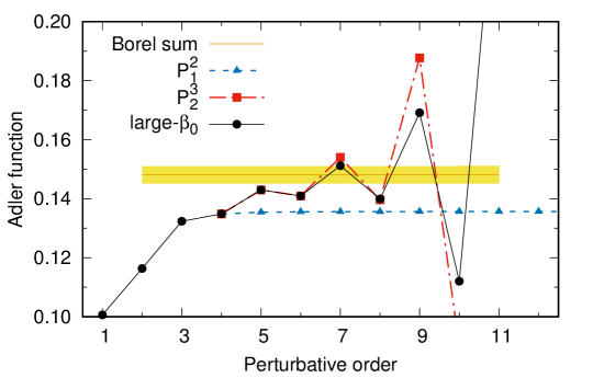
Figure 1: Results for the perturbative expansion of the Adler function in large-$\beta_{0}$ (solid line) and using the $P_{1}^{2}(u)$ (dashed line) and $P_{2}^{3}(u)$ (dot dashed line). The result of the Borel sum of the series is displayed with a band that represents its ambiguity. In all figures we use $\alpha_{s}(m_{\tau}^{2})=0.316\pm 0.010$ [49].

Using the same amount of information, we could consider the $P^{N}_{N+1}(u)$ sequence with the $P^{1}_{2}(u)$ and $P^{2}_{3}(u)$ its firsts elements. As we observed before, two-pole approximants yields better convergence ranges (by capturing the sign-alternating feature of the Borel series) so we should expect better $c_{5,1}$ and $c_{7,1}$ predictions for this sequence. We actually find $c_{5,1}=1770$ and $c_{7,1}=102,889$ respectively, a better determination than their $P_{N}^{N+1}(u)$ counterparts.

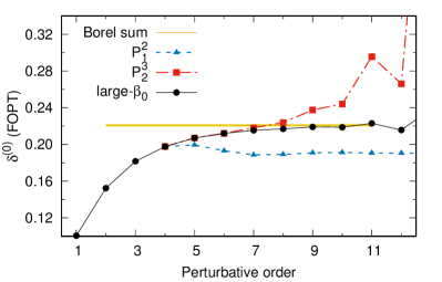
(a) $\delta^{(0)}$, FOPT.

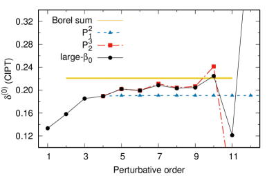
(b) $\delta^{(0)}$, CIPT.

Figure 2: Results for $\delta^{(0)}$ order by order in perturbation theory for large-$\beta_{0}$ (solid line) and for the $P_{1}^{2}(u)$ (dashed line) and $P_{2}^{3}(u)$ (dot dashed line) in FOPT (left) and CIPT (right). The Borel sum of series with its ambiguity is shown as the horizontal band.

It is thus interesting to investigate systematically the convergence of the Padé sequence with respect to $N$. In order to quantify the quality of the prediction of coefficients not used as input we define the relative error as

$$\sigma_{\rm rel}=\left|\frac{c_{n,1}^{P}-c_{n,1}}{c_{n,1}}\right|,$$ (32)

where $c^{P}_{n,1}$ is the coefficient extracted from the Padé approximant. If the PA sequence converges, the parameter $\sigma_{\rm rel}$ should tend to zero as $n$ grows.

In Fig. 3 we show the behavior of the relative error of the estimate of the $c_{2N+3,1}$ coefficient for the sequence $P_{N}^{N+1}$ as a function of $N$. Being the Adler function in large-$\beta_{0}$ a meromorphic function, the Pommerenke’s theorem ensures the convergence for a larger set of PA sequences than the $P_{N}^{N+1}$. To show this excellent global convergence pattern, we collect in Fig. 3 few of the closest-to-diagonal sequences, in particular the $P^{N+1}_{N}$, $P_{N}^{N}$, $P_{N+1}^{N}$, and $P_{N+3}^{N}$.

The results are qualitatively similar for all sequences: in all cases the convergence to the exact results happens fast as $N$ grows. We observe in Fig. 3 that the improvement once $N$ is increased by one unity is often of about one order of magnitude or more (notice the log scale of the plot). There are a few outliers where increasing $N$ by one unity does not represent an improvement, or even makes the relative error larger. A close scrutiny of the particular approximants reveals why this is so. For meromorphic non-Stieltjes functions, it is a feature of the Pommerenke’s theorem [26, 27] that the convergence pattern can be altered by the presence of defects, transients poles almost cancelled by a close-by zero as it is clearly noticed after observing the convergence pattern of the pole positions for the $P^{N}_{N+1}$ sequence: $P^{1}_{2}(u)$ has poles at $u=-0.56$ and at $u=0.89$; $P^{2}_{3}(u)$ at $u=-0.86$ together with a couple of complex-conjugated (CC) poles at $u=1.43\pm 0.46i$ — notice the stability of the UV pole which is driving the large-order behavior of the series (since it is always the closest to the origin)— then, $P^{3}_{4}(u)$ contains poles at $u=-0.85$, the CC poles at $u=1.40\pm 0.47i$ and an extraneous new pole closer to the origin at $u=-0.3991$. This last one, which would eventually spoil the convergence, is a new pole and it is actually canceled by a close-by zero at $u=0.3989$ effectively reducing the order of this approximant to a $P^{2}_{3}$. A similar feature is observed for the second and fifth elements of the $P^{N}_{N+3}$ sequence. In this last case, the cancellation among zero and pole is of the order of $10^{-13}$, i.e., the residue of the spurious pole is ${\cal O}(10^{-13})$. Identifying these cancelations will be important in the obtention of the final results of this paper.

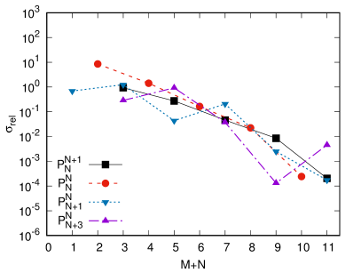
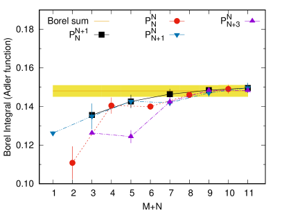
Figure 3: Results for four different Padé sequences in the ${\overline{\rm MS}}$ scheme. (a) Relative error of the first forecast coefficient of the Adler function, as defined in Eq. (32). (b) Results for the Borel sum, Eq. (10). The horizontal band gives the imaginary ambiguity of the true value.

When $N=4$, in all sequences the results are better by a few orders of magnitude compared to the first PA in each sequence. We remark that the convergence of some of these sequences was already studied in Ref. [30] and we confirm and extend their results.

In addition, PAs can be used as a way to resum the original series. In our case, the Borel integral can be performed with the reconstructed PAs using Eq. (10) in order to produce an estimate for the Borel sum of the series. The results for the Borel sum of the series also approach the true value when the order $N$ is increased, as can be seen in Fig. 3. As expected, the approximation becomes increasingly better, but it is also worth noting that the error is significantly reduced only after a relatively large value of $N$ is employed.

All in all, we arrive to the observation that PAs with larger values of $N$ tend to have poles that can be identified with the leading renormalons — at least for the ones that are closer to the origin in a hierarchical way [27]— and this is enough to yield a good approximation to the series coefficients and the Borel integral. In all cases, however, realistic values of $N$ ($N=1$ for $P_{N}^{N+1}$ and $P_{N+1}^{N}$ and $N=0$ for $P_{N+3}^{N}$) still do not provide a good approximation, as can be seen in Figs. 1, 2, 3 and 3. Since in full QCD only the first four coefficients of the Adler function are known it would be desirable to obtain a better approximation for these lower values of $N$. In the next section we discuss how scheme variations can be used to that end.

4.1.2 Scheme variations

The exact result for the Borel transformed Adler function in large-$\beta_{0}$, Eq. (22), displays explicitly an important property: the residues of the renormalon poles are scheme dependent but their position is not. Here we exploit this feature in order to improve upon the results of the previous section.

One of the difficulties in using PAs with a small number of parameters is the fact that they must mimic an infinite tower of renormalon poles and their complicated interplay with a set of only a few poles. In the ${\overline{\rm MS}}$, in lower orders, the first UV and IR poles give sizeable contributions to the coefficients [18, 25]. However, using schemes with negative values of $C$ the Borel transform becomes much more dominated by the first UV pole, due to the factor of $e^{(C+5/3)u}$, and the sign alternation should show up at very low orders. Because of this dominance, it becomes easier for a PA to reproduce such a series (we will elaborate on that below). Of course, negative values of $C$ entail larger values of $\hat{\alpha}_{s}$ [36], as per Eq. (29). These schemes are therefore bad for perturbative calculations but they are very useful, for example, to obtain estimates for the Borel sum of the series, since this is a scheme-independent result. Finally, the results for the coefficients with negative $C$ values can be translated to the ${\overline{\rm MS}}$ using the relation between the two couplings, and we will show that this leads to better results for the predicted higher order coefficients in ${\overline{\rm MS}}$.

For definiteness, we will work with $C=-5/3$ which cancels exactly the exponential in Eq. (22). In this scheme the central value of the coupling is $\hat{\alpha}_{s}(m_{\tau})=0.5074$. The expansion of the Adler function in the large-$\beta_{0}$ limit for $C=-5/3$ reads ($N_{f}=3$)

$$\widehat{D}_{L\beta}^{(C=-5/3)}(a_{Q})=\hat{a}_{Q}-2.194\,\hat{a}_{Q}^{2}+18.10\,\hat{a}_{Q}^{3}-139.0\,\hat{a}_{Q}^{4}+1610\,\hat{a}_{Q}^{5}-20,759\,\hat{a}_{Q}^{6}+\cdots$$ (33)

We remark that, as expected, the sign alternation sets in much earlier, in this case it starts from the second coefficient. The exact result for the Adler function in the large-$\beta_{0}$ limit for $C=-5/3$ can be seen in Fig. 4. It becomes clear that asymptoticity sets in also earlier due to the much larger value of the expansion parameter, $\hat{\alpha}_{s}$.

Let us consider again the Padé $P_{1}^{2}(u)$, but now in the scheme $C=-5/3$. In this new scheme we find

$$P_{1}^{2}(u)=\frac{0.2798+0.0455\,u+0.1899\,u^{2}}{0.8790+u},\qquad(C=-5/3).$$ (34)

Now, for the coefficient $c_{5,1}$ the result is $1423$, to be compared with the exact value $1610$ in Eq. (33), a relative error of only $12\%$ — this is an improvement of about an order of magnitude with respect to the result in the ${\overline{\rm MS}}$. The result for $c_{6,1}$, one order higher, is still very good: $-18,212$, just a $12\%$ relative error. Also, this $P_{1}^{2}(u)$ already displays a pole at $-0.8790$, close to the leading UV renormalon, and which reproduces the sign alternation of the coefficients. Finally, the Borel integral gives now 0.1416, much closer to the exact value (which is $0.1481\pm 0.0030i$, shown in Fig. 3). In Fig. 4, we see that the agreement with the exact Adler function is good even at higher orders. Clearly, $P_{1}^{2}(u)$ in this scheme provides a much more accurate prediction of the true function than its counterpart in the ${\overline{\rm MS}}$. The underlying reason is simple: without the exponential term, the position of the most prominent renormalon pole, the first UV, is much better determined in full agreement with the Pommerenke’s theorem [26, 27]. Furthermore, the suppression of the IR-pole residues simplify the interplay of the poles. Enlarging the sequence will only improve on the results.

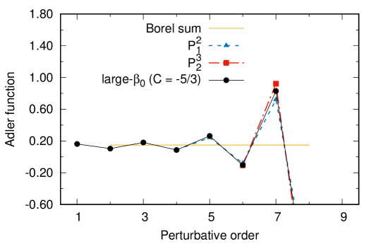
Figure 4: Perturbative expansion of the Adler function in large-$\beta_{0}$ in a scheme with $C=-5/3$ (solid line) and using the $P_{1}^{2}(u)$ (dashed line) and $P_{2}^{3}(u)$ (dot dashed line). The scheme-invariant result for the Borel sum of the series is the same as in Fig. 1. The value of the strong coupling in this scheme is $\hat{\alpha}_{s}(m_{\tau})=0.5074$ (see text).

Actually, for $C=-5/3$, the improvement for the $P_{2}^{3}(u)$ is only modest. We find

$$P_{2}^{3}(u)=\frac{0.2299-0.2080\,u+0.0769\,u^{2}-0.1283\,u^{3}}{(0.8757-u)(0.8248+u)},\qquad(C=-5/3)\,,$$ (35)

whit a prediction of the 7th coefficient has now a relative error of $10\%$ and pretty stable position of the pole closest to the origin: $-0.8248$. The Borel integral is again well predicted: $0.1394+0.0048i$.

For the next element in the sequence, $P_{3}^{4}(u)$, the prediction of the 9th coefficient has an error of mere $0.19\%$, about two orders of magnitude better than in the ${\overline{\rm MS}}$. Interestingly, for the first time, this PA has two poles close to $u=-1$, one at $-1.1312$ and a second at $-0.9385$ which mimics the fact that the leading UV pole is, actually, a double pole. It also has a pole at $1.788$, rather close to the location of the first IR pole, which lies at $u=2$. Finally, its Borel integral is also almost on top of the true one: $0.1476\pm 0.0084\,i$, the real part is off by only 0.3%.

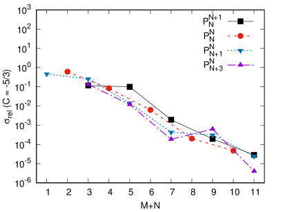
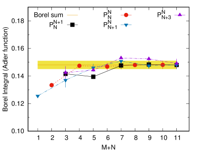
Figure 5: Results for different Padé sequences in a scheme with $C=-5/3$. The scales are the same as in Fig. 3 to facilitate the comparison. (a) Relative error of the first forecast coefficient of the Adler function. (b) Results for the Borel sum, Eq. (10).

Again, this excellent convergence pattern is not particular for this sequence. In Fig. 5 we show the relative error of the first predicted coefficient using the same four sequences of Fig. 3. The comparison with the results in the ${\overline{\rm MS}}$ clearly shows the advantage of using less perturbative schemes. For instance, the results for $P_{N}^{N+1}$ for $N=1$ are as good as those of the ${\overline{\rm MS}}$ with $N=3$, but require four parameters less. The results for the scheme-independent Borel sum predicted by these Padé sequences follow suit and are also significantly better than in the ${\overline{\rm MS}}$, as Fig. 5 shows. We should remark that for most of the Padés the results are even better if $C$ is lowered below $-5/3$. This means that the improvement in the results should not be directly attributed to the cancellation of the exponential term but rather to the value of the argument of that exponential. It is well-known [26] that the pole positions of diagonal and near-diagonal PA to an exponential function share three characteristics: the location corresponds with the sign of the exponential argument (positive argument, positive location in the complex plane with positive real part, and vice-versa), as soon as the PA order increases, the poles move further away from the origin, and finally for a given PA, the position of its poles is located within an area defined by its “order star” (cf. Ref. [26] for further definitions). These implies that as soon as the scheme is less perturbative, the PA poles responsible for the exponential term accumulate in the UV region further away as the PA order increases, isolating the rest of the poles coming from the non-exponential term, in particular the dominant UV double pole. On the contrary, for more perturbative schemes, PA poles will accumulate in the IR region and shadow the UV pole. From this perspective it is then natural to expect better convergence with respect to series coefficients and the Borel integral for the less perturbative schemes. It is apparent as well that the $C$-scheme analysis sheds light on the analytical structure of the Adler function in a clear way.

Let us now translate the results obtained in the scheme with $C=-5/3$ to the ${\overline{\rm MS}}$. The expansion of Eq. (29) gives the following perturbative relation between the different schemes

$$\hat{a}_{Q}=a_{Q}+\frac{C\beta_{1}}{2}a_{Q}^{2}+\Big{(}\frac{C\beta_{1}}{2}\Big{)}^{2}a_{Q}^{3}+\Big{(}\frac{C\beta_{1}}{2}\Big{)}^{3}a_{Q}^{4}+\cdots,$$ (36)

where on the r.h.s we have $a_{Q}$ in the ${\overline{\rm MS}}$ and on the l.h.s. $\hat{a}_{Q}\equiv a_{Q}^{C}$. Applying this perturbative relation to an expansion such as Eq. (33) one is able to reconstruct the ${\overline{\rm MS}}$ result from its counterpart in a scheme with a different $C$ value. Performing this procedure for the results of $P_{1}^{2}(u)$, $P_{2}^{1}(u)$ and $P_{2}^{3}(u)$ constructed at $C=-5/3$ leads to much better predictions of the higher order coefficients, as Tab. 1 confirms. The predictions are far superior to those obtained when the PA is constructed directly in the ${\overline{\rm MS}}$.

Table 1: Coefficients of the Adler function in the large-$\beta_{0}$ approximation in the ${\overline{\rm MS}}$ scheme. The first row gives the exact values. Darker rows show the results obtained from $P_{1}^{2}(u)$, $P_{2}^{1}(u)$ and $P_{2}^{3}(u)$ constructed in a scheme with $C=-5/3$ and later evolved to ${\overline{\rm MS}}$ using Eq. (36). For comparison, we also display the results obtained through the use of these PAs constructed directly in the ${\overline{\rm MS}}$ (second, fourth and sixth rows).

	$c_{5,1}$	$c_{6,1}$	$c_{7,1}$	$c_{8,1}$	$c_{9,1}$
large-$\beta_{0}$ exact	$787.8$	$-1991$	$9.857\times 10^{4}$	$-1.078\times 10^{6}$	$2.775\times 10^{7}$
$P_{1}^{2}$ (${\overline{\rm MS}}$)	$52.33$	$137.9$	$4.358\times 10^{2}$	$1.605\times 10^{3}$	$2.186\times 10^{4}$
$P_{1}^{2}$ ($C=-5/3$)	$600.5$	$-2958.0$	$7.022\times 10^{4}$	$-1.134\times 10^{6}$	$2.382\times 10^{7}$
$P_{2}^{1}$ (${\overline{\rm MS}}$)	$1770.1$	$-8123.9$	$61.277\times 10^{4}$	$-9.857\times 10^{6}$	$4.665\times 10^{8}$
$P_{2}^{1}$ ($C=-5/3$)	$1205.3$	$-1722.4$	$26.980\times 10^{4}$	$-2.024\times 10^{6}$	$1.234\times 10^{8}$
$P_{2}^{3}$ (${\overline{\rm MS}}$)	input	input	$1.257\times 10^{5}$	$-1.372\times 10^{6}$	$4.566\times 10^{7}$
$P_{2}^{3}$ ($C=-5/3$)	input	input	$1.311\times 10^{5}$	$-9.721\times 10^{5}$	$5.123\times 10^{7}$

4.1.3 Partial Padé Approximants

We have seen that Padé sequences appear to converge rather fast to the Borel transform of the Adler function, as expected following Pommerenke’s convergence theorem. In realistic applications, however, where one has only the first four coefficients of the series it may be necessary to employ a method to accelerate the convergence such as the scheme variation we discussed previously. In this section we will show that using knowledge about the position of the renormalon singularities significantly accelerates the convergence and yields excellent results even for the lowest approximants. We then consider now partial Padé approximants (PPAs) as defined in Eq. (17).

Most of the effort done by the PAs in the previous sections was to locate the double pole at $u=-1$, and this had a cost of two series coefficients. It is then to expect that including the double pole in advanced should allow the approximants to unfold the subdominant renormalon poles. For the ${\overline{\rm MS}}$ scheme, a $\mathbb{P}^{2}_{1,2}(u)$ (imposing the double pole at $u=-1$), leads to a prediction of $c_{5,1}$ which is $60\%$ off, while $c_{5,1}$ from $\mathbb{P}^{1}_{2,2}(u)$ is $55\%$ off. This represents a significant improvement with respect to the PAs. Results are much better for $C=-5/3$ where the predictions reach precision better than $3\%$ for both. In both schemes, pole predictions suggest the subdominant renormalons to be located in the IR region. Using more series coefficients one identifies the $u=2$ as the first IR renormalon.

As we have seen, the Borel transform of the Adler function has indeed an IR single pole at $u=2$ and the next step towards improving precision would be to consider a $\mathbb{P}^{M}_{N,3}(u)$ including such pole. In this case, and for the ${\overline{\rm MS}}$ scheme, results improve since with a $\mathbb{P}^{2}_{1,3}(u)$ one gets $30\%$ of relative error on the $c_{5,1}$ determination, whereas $20\%$ is reached with the $\mathbb{P}^{1}_{2,3}(u)$. For the $C=-5/3$ scheme, the result is greatly improved since relative errors reach up to $1\%$ and $5\%$ respectively. In this scheme, even a Padé-type approximant with a fixed denominator at $(u+1)^{2}(u-2)$, a $\mathbb{P}^{M}_{0,3}(u)$, yields good results. In this sort of sequence, one can even study the convergence by looking systematically at the $c_{5,1}$ prediction for growing $M$. We find $35\%$, $7\%$, and $4\%$ relative error for $M=1,2,3$ respectively.

Unraveling the sub-subdominant renormalons is now more an art than a science since it is difficult to decide whether the second UV or the second IR should be considered. The decision comes from exploring systematically the residue of the predicted poles from previous approximants. We observe that they predict an IR (double) pole at around $u=3$ with large residue. As such, it contributes largely to the series coefficients. The next step will be then to consider $\mathbb{P}^{M}_{N,5}(u)$ including this double pole where the polynomial $T_{5}(u)$ of Eq. (17) is constructed such as to reproduce the first five poles of the Borel transformed Adler function

$$T_{5}(u)=(u+1)^{2}(u-2)(u-3)^{2}.$$ (37)

We can then study near diagonal sequences akin to the ones we discussed in the previous section, e.g., $\mathbb{P}_{N,5}^{N+1}(u)$, $\mathbb{P}_{N+1,5}^{N}(u)$, or $\mathbb{P}_{N,5}^{N}(u)$. It is expected that these sequences should yield much better results since the perturbative series is dominated at intermediate and large orders by the poles closest to the origin.

We start with results for the sequence $\mathbb{P}_{N,5}^{N+1}(u)$ constructing the PPAs in the ${\overline{\rm MS}}$ scheme. The relative error of the the coefficient $c_{5,1}$ obtained from $\mathbb{P}_{1,5}^{2}(u)$ is 12 times smaller than the one from $P_{1}^{2}(u)$. The four coefficients used to fix the parameters of $\mathbb{P}_{1,5}^{2}(u)$ provide enough information to obtain a good approximation even after asymptoticity has set in — the 10th coefficient is predicted with a relative error of only $20\%$. This reproduction of the series is achieved by generating a pole at 1.750. Results from $\mathbb{P}_{2,5}^{3}(u)$ are so similar to the original function that they cannot be distinguished by eye. The approximant $\mathbb{P}_{2,5}^{3}$ has a pair of complex poles at $2.854\pm 0.992\,i$ which, again, appear due to the fact that the meromorphic function being approximated is not of the Stieltjes type.

The use of the scheme with $C=-5/3$ accelerates the convergence and now the results from $\mathbb{P}_{1,5}^{2}(u)$ cannot be visually distinguished from the exact ones (we therefore refrain from showing them explicitly). Relative errors for the $c_{5,1}$ are of the order of $0.7\%$ while for the tenth coefficient it is only about $2\%$. This excellent convergence is not unique for the $\mathbb{P}_{N,5}^{N+1}(u)$ sequence since for the subdiagonal one, $\mathbb{P}_{N+1,5}^{N}(u)$, results are basically indistinguishable. This is so that even a Padé-type sequence $\mathbb{P}_{0,5}^{N}(u)$ converges nicely and the systematic prediction of the series coefficients with increasing power $N$ yields a way to ascribe a theoretical or systematical error. $\mathbb{P}_{0,5}^{N}(u)$ with $N=2,3$ predict $797.8$ and $792.3$ respectively. Taking the difference among them as a way to estimate the error results into a prediction $792.3\pm 5.5$ which nicely agrees with the true coefficient $787.8$. Other results obtained from these approximants for FOPT and CIPT, as well as the Borel sum are as impressive as those for the Adler function and we refrain from quoting them explicitly.

At this point, two comments are in order. If, instead of considering double poles for the second IR pole and the leading UV pole in Eq. (37), we use simple poles the results are worsened. The coefficient $c_{5,1}$ obtained from $\mathbb{P}_{1,3}^{2}(u)$ using $T_{3}(u)=(u+1)(u-2)(u-3)$, changes from $847.9$ to $594.1$, to be compared with the exact value 787.8. The reason for this worsening is simple: fixed poles with wrong exponent forces the approximant to spend series coefficients to determine the correct exponents, with an associated loss of prediction power. This fact is nicely illustrated by $\mathbb{P}_{1,3}^{2}(u)$ in the ${\overline{\rm MS}}$, which has $(u+1)(u-2)(u-3)(u-3.06)$ as denominator, showing clearly that the Padé must reproduce the double-pole nature of the second IR renormalon. A scheme variation helps again in this issue since $\mathbb{P}_{1,3}^{2}(u)$ for $C=-5/3$ has as a denominator $(u+1.04)(u+1)(u-2)(u-3)$, with the extra pole very close to the first (and dominant) UV pole, emulating its double pole nature.

This shows that simply fixing poles at the correct location but with the wrong multiplicity does not represent necessarily an improvement over the situation where the poles are left free. An intermediate case where only the pole at $u=3$ has an incorrect exponent does yield improved results compared to the ordinary Padé approximants. This is in agreement with the findings of Ref. [25] where it was shown that imposing the correct structure of the first two leading poles is sufficient to achieve a good description of the large-$\beta_{0}$ Adler function. Actually, in the language of Padé approximants employed here, both the “reference model” and the “alternative model” of Ref. [25] can be thought of as a $\mathbb{P}_{0,5}^{6}(u)$, i.e., with full denominator fixed in advanced.

The main observation that can be drawn here is that having information about the first two or three renormalon poles is largely sufficient to achieve an excellent reconstruction of the series even with only four coefficients available (this conclusion is in agreement with Ref. [25]). Notice that even though we use large denominators, we still allow the approximants to have free poles. This helps them to improve on the convergence as free poles accommodate in an effective way the rest of the renormalon contributions.

4.1.4 D-log Padé approximants

While information on pole positions yields a clear improvement in the acceleration of convergence, the precise knowledge on pole positions can be, in realistic situations, scarce. Moreover, knowing the multiplicity of poles is also important. Additionally, some functions present branch point singularities, which may render their approximation by Padés less effective. As discussed in the Introduction, in such situations, other strategies may be pursuit. In particular, the D-log Padé approximants of Eqs. (18) and (19) and their extension in Eqs. (20) and (21) can result optimal.

The original philosophy of the simplest D-log Padé approximant is to perform a PA not to $f(z)$ but to $F(z)=\frac{\rm d}{{\rm d}z}\log[f(z)]$. Assuming the original function has a singularity at $z=\mu$ (a pole or a branch cut) the evaluation of the outcome at $z=\mu$ provides a way to extract, from the series coefficients, the multiplicity $\gamma$ of the singularity at $\mu$. Here, if $\gamma$ is an integer or not becomes irrelevant which makes the D-log Padés particularly interesting to approximate functions with branch cuts. Of course, by unfolding the procedure one obtains the non-rational approximant ${\rm Dlog}_{N}^{M}(z)$ of Eq. (19) to the function $f(z)$ which, after reexpansion, returns the series coefficients.

The simplest D-log approximant for the Borel transform of the Adler function, ${\rm Dlog}^{1}_{0}(u)$, requires $c_{2,1}$ and $c_{3,1}$ and reads:

$${\rm Dlog}^{1}_{0}(u)=f(0)e^{0.69u+1.31u^{2}}\,.$$ (38)

After reexpanding, ${\rm Dlog}^{1}_{0}(u)$ predicts both $c_{4,1}$ and higher coefficients and it does it rather accurately, taking into account the little information that was used. Still, no sign-alternation is observed. Going up to ${\rm Dlog}^{2}_{0}(u)$, the prediction improves a lot and not only the sign-alternation is now reproduced, but also the relative error for the $c_{5,1}$ is around $40\%$ (better for the next $c_{6,1}$ which is just $10\%$ off). At the same order, a ${\rm Dlog}^{1}_{1}(u)$ yields even better results, being only $16\%$ off for $c_{5,1}$, with the correct sign-alternation and a good prediction for $c_{6,1}$ as well, as can be seen in Fig. 6. Using this simplest scenario, with minimum information, the ${\rm Dlog}^{1}_{1}(u)$ is the approximant that better predicts $c_{5,1}$ among the approximants presented in this work so far.

Information on known singularities can be straightforwardly used with the partial D-log Padés, $\mathbb{D}{\rm log}^{M}_{N}(z;\mu)$, of Eq. (20). The singularity closest to the origin in the Borel transform Adler function is the UV pole at $u=-1$. We then consider a PA to $(1+u)\frac{\rm d}{{\rm d}u}\log[f(u)]$ instead, and construct the respective $\mathbb{D}{\rm log}$ approximant to $f(u)$. Even with the simplest $\mathbb{D}{\rm log}^{1}_{0}(u;-1)$ the sign-alternation of the series coefficient is recovered, a clear indication of an improvement on the series’ reconstruction. The unfolded approximant reads

$$\mathbb{D}{\rm log}^{1}_{0}(u;-1)=f(0)\frac{e^{3.32\,u}}{(1+u)^{2.6}}$$ (39)

which has a branch point at $u=-1$ but with a good prediction on the actual multiplicity of the first UV renormalon (which is a double pole in large-$\beta_{0}$).

For the next order, two choices can be considered, the diagonal $\mathbb{D}{\rm log}^{1}_{1}(u;-1)$ and the $\mathbb{D}{\rm log}^{2}_{0}(u;-1)$. As it is clear from the definition in Eq. (20), $F(z)$ is to a good approximation, a rational function. Then, the diagonal $\mathbb{D}{\rm log}^{1}_{1}(u;-1)$ is the optimal choice, specially if one is heading towards determining the multiplicity $\gamma$. In this case, the unfolded approximant reads

$$\mathbb{D}{\rm log}^{1}_{1}(u;-1)=\frac{881379.40}{(4.02-u)^{10.67}(1+u)^{1.96}}\,,$$ (40)

and, upon expansion, predicts the series coefficients for the Borel transform with unprecedented precision for coefficients up to $c_{10,1}$, with relative errors amounting to mere $0.8\%,6\%,2\%,3\%,2\%,1\%,1\%$ for the coefficients $c_{4,1}$ to $c_{10,1}$ in that order. The excellent results for this approximant can also be seen in Fig. 6. A key point in this extraordinary success is the excellent reproduction with very little information of the multiplicity of the first UV pole, as can be seen by the fact that $\gamma=1.96$ for the $\mu=-1$ in Eq. (40), while the other branch cut effectively emulates the tower of IR poles in the Borel transform. The result is so good that including $c_{4,1}$ to construct the $\mathbb{D}{\rm log}^{1}_{2}(u;-1)$ yields only a marginal improvement (predicting $c_{5,1}$ with a $5\%$ of relative error, for example).

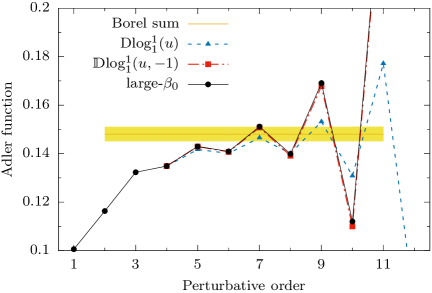
(a) Adler function.

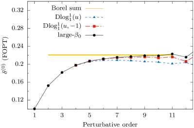
(b) $\delta^{(0)}$, FOPT.

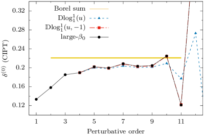
(c) $\delta^{(0)}$, CIPT.

Figure 6: Results from the use of the approximants ${\rm Dlog}^{1}_{1}(u)$ and $\mathbb{D}{\rm log}^{1}_{1}(u;-1)$ in large-$\beta_{0}$. (a) Perturbative expansion of the Adler function. (b) $\delta^{(0)}$ in FOPT, and (c) $\delta^{(0)}$ in CIPT.

It is then clear the D-log Padés are able to go much beyond ordinary PAs in reproducing the main analytical features of the Borel transformed Adler function in large-$\beta_{0}$. The success of this approximants can be understood by examining the function $\frac{\rm d}{{\rm d}z}\log[f(z)]$. Let us write the explicit result for the first leading poles, obtained from considering only the first term in the sum of Eq. (22),

$$F(u)=\frac{{\rm d}}{{\rm d}u}\log\left(B[\widehat{D}](u)\right)=C+\frac{5}{3}-\frac{2}{1+u}+\frac{2}{2-u}+\frac{2}{3-u}+\cdots$$ (41)

This shows that in the D-log Padés the function being approximated is strictly a rational function, with simple poles. The exponential function present in the Borel transform disappears and the approximants do not have to reproduce it. In a sense, the D-logs strategy realizes a situation similar to that of a scheme with $C=-5/3$ which cancels the exponential of the Borel transform but with the additional benefit that $F(z)$ has only simple poles. Their success is, therefore, not so surprising. We can also expect that sequences of PAs that depart significantly from the diagonal will have a slower convergence to $F(u)$ and will, accordingly, lead to a worse approximation of $B[\widehat{D}](u)$.

Finally, the inclusion of information about the position of more than one pole can be done in the context of D-log Padés by using a partial Padé approximant to $F(z)$, with as many poles fixed as one desires. Using in the denominator of such a PPA $T_{7}(u)=(2-u)(3-u)^{2}(1+u)^{2}(3+u)^{2}$, and with $c_{2,1},c_{3,1}$ and $c_{4,1}$ as input one predicts the series’s coefficients with precision better than $0.1\%$.

In conclusion, the D-log Padés are shown to be an effective way to improve the convergence of the approximation and gain information about higher orders. In some sense, they are better than the scheme transformations since they do not rely on a specific value of $C$. We turn now to the use of the techniques described here for the function $\delta^{(0)}_{\rm FO}$ in large-$\beta_{0}$, before applying them to full QCD.

4.2 Padé approximants to $\delta^{(0)}$

We learn from the application of Padé approximants to the Borel transform of the Adler function that one of the difficulties is the disentanglement of the leading renormalons. The success of the use of scheme variations lies partially in this fact, since the method allows for an enhancement of the leading UV pole with respect to the leading IR pole at $u=2$. The Borel transform of $\delta^{(0)}$, Eq. (23), on the other hand, does not have the pole at $u=2$. The leading UV renormalon is therefore more isolated from the IR ones. It can be expected that the use of Padé approximants directly to this Borel transform should yield better and more stable results than in the case of the Adler function. In this section we exploit this route. Since general properties of the Padé approximants were discussed in the previous section, we will focus here on the practical problem of forecasting the unknown coefficients given that only the first four are known exactly — in order to simulate the case of real QCD.

Let us note that a rational approximant to $\delta^{(0)}$ contains enough information to allow for a full reconstruction of the Adler function. The coefficients $c_{n,1}$ can easily be read off from the FOPT expansion of $\delta^{(0)}$ as

$${\delta}^{(0)}_{\text{FO},L\beta}(a_{Q}) =\ c_{1,1}\ a_{Q}+(3.563\ c_{1,1}+c_{2,1})\ a_{Q}^{2}+(1.978\ c_{1,1}+7.125\ c_{2,1}+c_{3,1})\ a_{Q}^{3}$$

$$+(-45.31\ c_{1,1}+5.934\ c_{2,1}+10.69\ c_{3,1}+c_{4,1})\ a_{Q}^{4}+\cdots$$ (42)

Additionally, in large-$\beta_{0}$, Eq. (23) can be used to extract the Borel transformed Adler function from that of $\delta^{(0)}$.

We start here by applying Padé approximants directly to the series in $\alpha_{s}/\pi$, given by Eq. (25). As we have observed, the FOPT series in large-$\beta_{0}$ is rather well behaved and, at intermediate orders, its asymptotic nature is not visible yet. This is mapped into a simpler analytic structure in the Borel plane. It is therefore likely that in this case the approximation of the series by Padé approximants in $a_{Q}$ will lead to a better description than in the case of the Adler function. In Tab. 2, we display the Adler function coefficients that are obtained from the application of Padé approximants directly to the FOPT expansion of $\delta^{(0)}$. To simulate the situation of real QCD, in the first two rows, we attempt to forecast $c_{4,1}$, while in the last three we use $c_{4,1}$ as input. The main observation is that the results for the coefficients that are not used as input are quite good and stable. The sign alternation of the series is correctly predicted by all the Padés and good consistency between the results using three and four coefficients as input is achieved. The results are therefore quite remarkable.

Let us examine one of the PAs in more detail. For $P_{1}^{2}$, which uses only the first three coefficients as input, we find

$$P_{1}^{2}(a_{Q})=\frac{0.1779\,a_{Q}-0.0895\,a_{Q}^{2}}{0.1779-a_{Q}}.$$ (43)

First, we see that the series obtained from such a Padé is convergent (since $a_{\tau}\approx 0.1$) and does not reproduce the factorial growth of the coefficients. The pole that appears around $a_{Q}\approx 0.18$ is, however, rather stable — it does not seem to be transient in nature and is present in all the approximants to ${\delta}^{(0)}_{\text{FO},L\beta}$. It may be worth noting that the pole is in the IR and corresponds to a scale of $\sim 650$ MeV. It may, therefore, be related to IR physics but we refrain from further speculation regarding the nature of this pole. An estimate for the sum of the series can be obtained simply using $a_{\tau}=0.316/\pi$ in Eq. (43) to give $P_{1}^{2}(a_{\tau})=0.2198$. This result is also in very good agreement with the value obtained from the Borel integral of the exact large-$\beta_{0}$ result, which gives $0.2208\pm 0.0039$. Even better results can be obtained from the PAs that use four coefficients as input, as shown in the last three rows of Tab. 2.

Table 2: Adler function coefficients extracted from PAs $P_{M}^{N}(a_{Q})$ to the FOPT $\alpha_{s}/\pi$ expansion of $\delta^{(0)}$ in the large-$\beta_{0}$ limit.

	$c_{4,1}$	$c_{5,1}$	$c_{6,1}$	$c_{7,1}$	$c_{8,1}$	$c_{9,1}$
Large-$\beta_{0}$ (exact)	$24.83$	$787.8$	$-1991$	$9.857\times 10^{4}$	$-1.078\times 10^{6}$	$2.775\times 10^{7}$
$P^{2}_{1}(a_{Q})$	$29.95$	$723.7$	$-703.4$	$7.405\times 10^{4}$	$-5.871\times 10^{5}$	$1.649\times 10^{7}$
$P^{1}_{2}(a_{Q})$	$28.66$	$728.2$	$-874.3$	$7.554\times 10^{4}$	$-6.224\times 10^{5}$	$1.703\times 10^{7}$
$P^{3}_{1}(a_{Q})$	input	$740.0$	$-1363$	$7.956\times 10^{4}$	$-7.211\times 10^{5}$	$1.851\times 10^{7}$
$P^{2}_{2}(a_{Q})$	input	$749.3$	$-1444$	$8.169\times 10^{4}$	$-7.514\times 10^{5}$	$1.917\times 10^{7}$
$P^{1}_{3}(a_{Q})$	input	$743.6$	$-1393$	$8.035\times 10^{4}$	$-7.321\times 10^{5}$	$1.875\times 10^{7}$

We now turn to PAs to the Borel transformed $\delta^{(0)}$. The results are improved when compared with PA to $B[\widehat{D}]$, although the improvement is far from spectacular. For $c_{5,1}$ we find the values $263.9$, $603.6$, and $1024$ from $P_{2}^{1}$, $P_{3}^{0}$, and $P_{1}^{2}$ respectively, to be compared with $52.33$, $560.9$, and $1770.1$ from the same PAs to $B[\widehat{D}]$. Clearly, one must resort to the other methods discussed in the previous section in order to accelerate the convergence. Again, D-Log Padés turn out to be the optimal way to improve the convergence while remaining completely model independent. Their success can be understood from the a study of the function $F(u)=\frac{{\rm d}}{{\rm d}u}\log\left(B[\delta^{(0)}](u)\right)$, as is in the case of the Adler function. Here we find, retaining only the first term in the sum of Eq. (22),

$$F(u) =\frac{{\rm d}}{{\rm d}u}\log\left(B[\delta^{(0)}](u)\right)$$

$$=C+\frac{5}{3}+\pi\cot(\pi u)-\frac{2}{1+u}+\frac{3}{3-u}+\frac{1}{4-u}+\frac{1}{1-u}+\frac{1}{2-u}-\frac{1}{u}+\cdots$$ (44)

The leading analytic structure of $F(u)$ is now even simpler than for the Adler function. The poles at $u=0$, $u=1$, and $u=2$ are exactly cancelled by the presence of $\pi\cot(\pi u)$ leaving only a leading UV pole at $u=-1$, an IR pole at $u=3$ and a subleading IR pole at $u=4$. It is therefore expected that the D-log Padés should perform even better in the present case.

We present results for the D-Log Padés applied to $B[\delta^{(0)}]$ in Tab. 3. These results also represent an improvement when compared to those of Sec. 4.1.4. The predictions for $c_{5,1}$ have a much smaller relative error, a factor of 2 to 5 times smaller than those obtained from the PAs to the Borel transformed Adler function. The sign alternation is well reproduced by the Padés with four coefficients used as input and their Borel integral provide excellent estimates for the true value of the series (we find, e.g., 0.2199 from $\text{DLog}^{1}_{1}(u)$). However, one must note that the results from the D-Log Padés applied to $B[\delta^{(0)}]$ are less good than those of Tab. 2. For example, the coefficient $c_{4,1}$ is wrong by a factor of about two while in Tab. 2 it is only a few percent off. Nevertheless, the description of the Borel transformed $\delta^{(0)}$ by D-Log Padés has the advantage that the factorial growth of the coefficients is reproduced and an asymptotic series is obtained, in line with the exact result.

We have checked that the results discussed in this section can be further improved by using information about the renormalons. For example, imposing the existence of the leading UV pole at $u=-1$ through the use of $\mathbb{D}{\rm log}_{1}^{1}(u;-1)$ leads to an almost exact reproduction of the series. We prefer, however, to remain as model independent as possible and we chose to focus here on the results obtained from the most model independent methods (PAs and D-log Padés). By using $\delta^{(0)}$ and its Borel transformed, these model-independent methods lead to results as good as those obtained from the Adler function imposing information on the renormalons.

Table 3: Adler function coefficients extracted from D-Log Padé approximants, ${\rm Dlog}_{M}^{N}(u)$, constructed to $B[\delta^{(0)}](u)$ in the large-$\beta_{0}$ limit.

	$c_{4,1}$	$c_{5,1}$	$c_{6,1}$	$c_{7,1}$	$c_{8,1}$	$c_{9,1}$
Large-$\beta_{0}$ (exact)	$24.83$	$787.8$	$-1991$	$9.857\times 10^{4}$	$-1.078\times 10^{6}$	$2.775\times 10^{7}$
$\text{Dlog}^{1}_{0}(u)$	$41.84$	$756.1$	$848.6$	$7.453\times 10^{4}$	$-3.284\times 10^{5}$	$1.498\times 10^{7}$
$\text{Dlog}^{0}_{1}(u)$	$44.43$	$776.1$	$1294$	$7.778\times 10^{4}$	$-2.502\times 10^{5}$	$1.538\times 10^{7}$
$\text{Dlog}^{2}_{0}(u)$	input	$650.2$	$-1824$	$6.319\times 10^{4}$	$-7.470\times 10^{5}$	$1.545\times 10^{7}$
$\text{Dlog}^{1}_{1}(u)$	input	$818.7$	$-2738$	$1.189\times 10^{5}$	$-1.663\times 10^{6}$	$4.495\times 10^{7}$
$\text{Dlog}^{0}_{2}(u)$	input	$594.9$	$-1974$	$5.560\times 10^{4}$	$-6.796\times 10^{5}$	$1.432\times 10^{7}$

We close this section with a visual account of the results discussed here. In Fig. 7(a), we display the $\delta^{(0)}$ FOPT and CIPT expansions obtained from the approximant $P_{2}^{2}(a_{Q})$, for which we show the coefficients up to $c_{9,1}$ in the 5th row of Tab. 2. The main observation is that, up to the 9th order, the result is strikingly similar to the exact ones (see, e.g., the black lines in Figs. 6(b) and 6(c)). However, the FOPT series thus obtained is convergent, and after the 8th order its result stabilizes around the sum of the series, which cannot happen in the exact results. This does not prevent the description from being excellent at intermediate orders, since the true value of the convergent series is very similar to the central value of the Borel integral of the exact results. For CIPT, similar observations hold and up the 9th order the result is almost indistinguishable from the exact ones. In particular, the fact that FOPT is the best approximation in large-$\beta_{0}$ is well reproduced. In Fig. 7(b), we display results for ${\rm Dlog}_{1}^{1}(u)$, for which the coefficients are given in the 5th row of Tab. 3. Again, visually, the results are almost identical to the exact ones. Now, both series are divergent, as is the case in the exact results, and this feature shows up after the 9th order, although the divergence, here, is more pronounced than in the exact large-$\beta_{0}$ case. In both cases, however, the approximants provide a good estimate for the first few unknown coefficients and give an excellent account of the series even though no information about the renormalons was used, in contrast with some of the results of Fig. 6(b) and 6(c)).

4.3 Summary and discussion

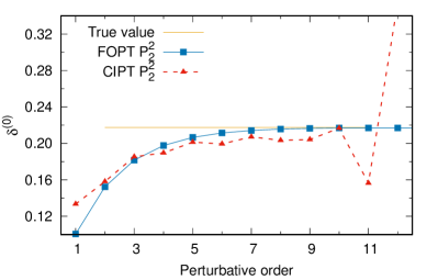
(a) $\delta(0)$ from $P_{2}^{2}(a_{Q})$.

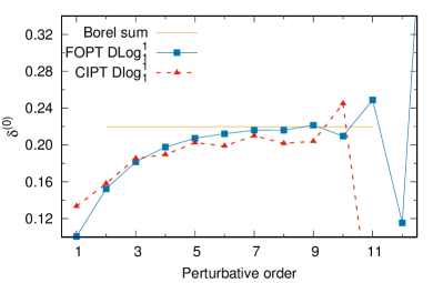
(b) $\delta(0)$ from ${\rm Dlog}_{1}^{1}(u)$.

Figure 7: Perturbative expansion of $\delta^{(0)}$ in FOPT and CIPT obtained from (a) $P_{2}^{2}(a_{Q})$ (5th row of Tab. 2) and (b) ${\rm Dlog}_{1}^{1}(u)$ (5th row of Tab. 3).

Here we summarize the main conclusions that can be drawn from the application of Padé theory to the results in the large-$\beta_{0}$ limit of QCD.

The application of the Padé approximants to the ${\overline{\rm MS}}$ Borel transformed Adler function in the large-$\beta_{0}$ limit displays convergence. With six or seven coefficients one is able to reproduce very well all the essential aspects of the original series: its higher order coefficients, its Borel sum, and even the position of the dominant renormalon poles. There are, however, outliers and it can happen that the next Padé in a given sequence does not make the results better. The existence of these outliers is well understood in the theory of Padés and we have been able to show for specific examples why this happens. All in all, convergence is always observed once an even larger number of parameters is added. Results using only four coefficients of the series to construct the Padés — which corresponds to the number of available coefficients in QCD — are, however, far from spectacular. In the absence of more coefficients, one must exploit strategies to improve the approximation of the original function.

In the case of the large-$\beta_{0}$, we have shown that using less perturbative schemes, which with our conventions corresponds to $C<0$, one is able to construct better approximants with the same number of parameters. This improvement is due to the fact that the Borel transform in these schemes becomes largely dominated by the leading UV pole: one observes the sign alternation earlier and the Padés can easily reproduce the main features of the analytical structure of the series. The specific choice $C=-5/3$ has the additional advantage of removing the term $e^{C+5/3}$ from the Borel transform, which makes it a strict rational function. As a by-product, we are able to devise a strategy to reveal the effects of the dominant UV pole. Constructing the series for $C<0$ the sign-alternation of the coefficients sets in much earlier, already from the second coefficient.

Next, we have seen that the use of partial Padé approximants, where the available information about the renormalon poles can be exploited, leads to significant improvements. However, it is important to use this information with care, since imposing the existence of a pole but with wrong multiplicity forces the Padé to “spend” series coefficients fixing the analytic structure of the given pole. If the information of the leading UV pole is used correctly, this leads to a significant improvement on the results. Finally, we find that imposing the structure of the first two leading renormalons leads to an almost perfect reproduction of the Adler function. This is in line with the renormalon models of Ref. [25].

We then investigated the use of D-log Padés. These are an interesting alternative having in mind applications to QCD, since they do not require that the function be meromorphic. Their application in large-$\beta_{0}$ was very successful and we can safely conclude that, given the limited information available, they are the best way to accelerate convergence of the procedure. We highlight the use of partial D-log Padés where only the existence of first UV pole is used as input. The results of such partial D-logs are truly impressive and lead to an almost exact reproduction of the Adler function in large-$\beta_{0}$ with an almost model-independent method. We were able to explain their success in terms of the analytic structure of the Borel transformed Adler function.

We then turned to approximants constructed to $\delta^{(0)}$. First, we have shown that PAs to the FOPT series in $\alpha_{s}/\pi$, contrary to the case of the Adler function, do lead to a very good reconstruction of the series at intermediate orders. In the case of $\delta^{(0)}$, since the FOPT series is rather well behaved and regular up to the 10th order (with terms that are consistently smaller than their predecessor) the approximation obtained from these Padés is very reasonable. We have then shown that good results can also be obtained from D-log Padé approximants constructed to $B[\delta^{(0)}]$. They are completely model independent and have the advantage that the factorial growth of the coefficients is automatically implemented. Both methods lead to good predictions for the true value of the series and are sufficient to conclude that FOPT is the best prescription in large-$\beta_{0}$. Again, the success of the method can be explained by the simpler analytic structure of the Borel transformed $\delta^{(0)}$ since it does not have the pole at $u=2$ and all other poles become simple (with the exception of the ones at $u=3$ and $u=4$).

The systematic study performed in the large-$\beta_{0}$ limit leads to strategies for impressive determinations of the higher order coefficients and the Borel sum of the Adler function and $\delta^{(0)}$ series. We were able to find methods to unravel dominant and subdominant poles, as well as to reorganize the available information in order to optimize the approximation by PAs and its variants. With these strategies at hand we can now perform a similar analysis in full QCD and present our final results.

5 The QCD case

In this section we will apply the techniques developed and tested in large-$\beta_{0}$ to the real case of QCD. Let us first remind what is known in this case. In perturbation theory, the Adler function expansion is known to five loops, hence to order $\alpha_{s}^{4}$ [21]. We would like to obtain predictions for the coefficients $c_{5,1}$ and higher. The first four coefficients of the Adler function in QCD, displayed in Eq. (8), already show a significant deviation from the large-$\beta_{0}$ results, although the coefficients of the $\delta^{(0)}$ FOPT expansion, Eq. (14), are closer to the their large-$\beta_{0}$ counterparts. The differences between full QCD and the large-$\beta_{0}$ limit also show up in the Borel transform. In QCD, we know that the Borel transform is no longer a meromorfic function. Although the renormalon singularities remain at the same position, anomalous dimensions of the operators and higher-order $\beta$-function coefficients now change their nature from poles to branch points. What is more, at every branch point there are confluent singularities [24, 18]. Experience shows that Padé approximants can be safely employed to approximate functions with branch cuts, but we no longer have convergence theorems to exploit, without further knowledge on the properties of these branch cuts.

Let us start with the simplest approximants: PAs constructed directly to the $\alpha_{s}/\pi$ expansion of the Adler function. We have discussed that in large-$\beta_{0}$ this was not the optimal strategy. Given that we have now only the first four coefficients, we start by building the PAs that would “postdict” the last known term of the series, $c_{4,1}$. From the approximants $P_{1}^{2}(a_{Q})$ and $P_{2}^{1}(a_{Q})$ we obtain the five-loop coefficients with $51\%$ and $67\%$ relative error, respectively. The coefficient $c_{5,1}$ is predicted to have quite low values $96.2$ and $50.5$. Our experience from large-$\beta_{0}$ already signals that this strategy is not optimal. If we construct approximants that now use $c_{4,1}$ as input we extract $c_{5,1}$ coefficients that can differ from the previously obtained by a factor of 9, indicating that the procedure is very unstable.

We then turn to the approximation of the Borel transformed Adler function, which proved to be more stable in large-$\beta_{0}$. Again, we first try to obtain a “postdiction” of $c_{4,1}$, using $P_{1}^{1}(u)$ and $P_{2}^{0}(u)$. The value of $c_{4,1}$ thus obtained has a relative error of about $26\%$, which is an improvement with respect to the previous method, and leads to predictions of $c_{5,1}\sim 280$. However, when we construct approximants that include the true value of $c_{4,1}$ as input, $P_{1}^{2}$, $P_{2}^{1}$, $P_{3}^{0}$, there is no sign of stability. The predictions for $c_{5,1}$ and higher order coefficients change substantially which, from our experience in large-$\beta_{0}$, signals that the approximants are not optimal. That only four coefficients is not enough for the usual Padé approximants to perform a stable prediction of the higher orders comes as no surprise, since this is what happens in large-$\beta_{0}$ even though the analytical structure of the Borel transform is simpler there. We must again resort to methods for the acceleration of the convergence of the procedure.

We start by investigating other renormalization schemes. Scheme variations in full QCD can also be performed using a single parameter $C$, through the generalization of Ref. [36] (to which we refer for further details). Based on the lessons from large-$\beta_{0}$ we rewrite the Adler function series in schemes with negative $C$, hence with larger values of the coupling. As an example, let us take again the value $C=-5/3$. The first four coefficients of the Adler function are now

$$\widehat{D}^{(C=-5/3)}(a_{Q})=\hat{a}_{Q}-2.110\,\hat{a}_{Q}^{2}+2.779\,\hat{a}_{Q}^{3}+19.87\,\hat{a}_{Q}^{4}+\cdots$$ (45)

There are marked differences in the coefficients when compared with Eq. (33). In contrast to the large-$\beta_{0}$ case, the series in QCD with negative $C=-5/3$ does not display a systematic sign alternation. It seems, therefore, that the UV singularity is less dominant than in large-$\beta_{0}$ and the pattern of signs indicate a more complicated interplay between the poles. Possibly, the IR poles give a larger contribution to the QCD series relatively to the large-$\beta_{0}$ case. This is in line with the results of the models of Refs. [18, 25]. In these models, the IR poles give larger contributions at intermediate orders and the systematic sign alternation sets in only at the 11th order. Since we are not able to unequivocally suppress the contribution of the IR poles, the strategy of using scheme variations to optimize the use of Padé approximants does not turn out optimal in QCD (although it corroborates, in part, the results of Refs. [18, 25]).

We resort then to the use of D-log Padés to obtain approximants to $B[\widehat{D}](u)$. Their use in full QCD is also well motivated, since they are designed for functions that have branch cuts. The use of D-log Padés to postdict $c_{4,1}$ leads to values with relative error of $54\%$ [${\rm Dlog}^{1}_{0}(u)$] and $21\%$ [${\rm Dlog}_{1}^{0}(u)$] which again signals that the procedure is not optimal. The use of an additional coefficient as input does not change this picture significantly, since it leads to unstable results for higher-order coefficients, which is understandable again due to the presence of confluent singularities.

Based on our experience from the large-$\beta_{0}$ limit, one is the led to conclude that model-independent approximants constructed to the Borel transformed Adler function are not robust enough in QCD with only the first four coefficients available. In large-$\beta_{0}$ the knowledge about renormalon singularities could be used to optimize the predictions. Here, however, we face additional difficulties. First, the available knowledge is more scarce. Only the first few renormalons (the leading UV, and the two leading IR) have had their branch cut structure investigated in detail [18, 55]. Second, the fact that now the renormalons become confluent singularities renders much more difficult the use of the available knowledge to devise optimized approximants. And, finally, it would be desirable to remain as model independent as possible. We therefore turn directly to the most successful model-independent strategy devised in large-$\beta_{0}$: the use of the FOPT series for $\delta^{(0)}$.

In large-$\beta_{0}$ approximants constructed to $\delta^{(0)}_{\rm FO}$ and $B[\delta^{(0)}]$ resulted optimal. The perturbative series for $\delta^{(0)}_{\rm FO}$ in large-$\beta_{0}$ and in QCD have rather similar coefficients. This means that the regularity of the series is preserved in QCD, which suggests that it can be well approximated by Padé approximants constructed directly to the series in $\alpha_{s}/\pi$. Furthermore, although Eq. (23) is strictly valid only in large-$\beta_{0}$, because it relies on the one-loop running of the coupling, modifications to this result would be solely due to higher-orders in the $\alpha_{s}$ evolution. We can therefore expect that a suppression of the leading IR singularity at $u=2$, as well as a suppression of all the other renormalons except for the ones at $u=3$ and $u=4$, would survive in full QCD and render this Borel transform more amenable to approximation by rational functions.

We start with Padé approximants applied to the $\alpha_{s}/\pi$ expansion of $\delta^{(0)}_{\rm FO}$. As before, we begin with a post-diction of $c_{4,1}$ using $P_{2}^{1}(a_{Q})$ and $P^{2}_{1}(a_{Q})$. The results for six higher-order coefficients obtained from these approximants are shown in Tab. 4. The relative error from the central values of $c_{4,1}$ is now $\sim 13\%$. This is quite remarkable when put into perspective since before the true value of $c_{4,1}$ was computed, a forecast of this coefficient using other methods and including additional information (taking into account known terms of order $\alpha_{s}^{4}N_{f}^{3}$ and $\alpha_{s}^{4}N_{f}^{2}$) yielded $c_{4,1}=27\pm 16$ [52, 53, 54], a central value which was $45\%$ off. This gives an idea of how powerful optimal PAs can be.

Table 4: QCD Adler function coefficients from PAs constructed to the $\alpha_{s}$ expansion of $\delta^{(0)}_{\rm FO}$.

	$c_{4,1}$	$c_{5,1}$	$c_{6,1}$	$c_{7,1}$	$c_{8,1}$	$c_{9,1}$	Padé sum
$P^{2}_{1}$	$55.62$	$276.2$	$3865$	$1.952\times 10^{4}$	$4.288\times 10^{5}$	$1.289\times 10^{6}$	0.2080
$P^{1}_{2}$	$55.53$	$276.5$	$3855$	$1.959\times 10^{4}$	$4.272\times 10^{5}$	$1.307\times 10^{6}$	0.2079
$P^{3}_{1}$	input	$304.7$	$3171$	$2.442\times 10^{4}$	$3.149\times 10^{5}$	$2.633\times 10^{6}$	0.2053
$P^{1}_{3}$	input	$301.3$	$3189$	$2.391\times 10^{4}$	$3.193\times 10^{5}$	$2.521\times 10^{6}$	0.2051

Inspecting the Padé approximants of the first two rows of Tab. 4 they reveal a pole around $a_{Q}=0.1973$, of similar nature to the one found in large-$\beta_{0}$. Additionally, $P_{2}^{1}$ has a pole far from the origin at $a_{Q}=7.25$. This makes their expansion around $a_{Q}=0$ similar and their predictions turn out to be almost degenerate. Therefore, a stronger test for stability comes with the use of $c_{4,1}$ as input, to obtain $c_{5,1}$ and higher. One could construct, for example, the approximant $P_{2}^{2}$. However, this approximant has a defect, in the sense discussed in Sec. 4.1.1, a pole and a zero that cancel almost exactly, effectively reducing the order of the approximant. Although its results are not completely inconsistent (e.g., $c_{5,1}$ turns out to be $242$) we have shown that it is wise to avoid approximants of this type and we will discard $P_{2}^{2}$. We turn then to the results obtained for $P_{1}^{3}$ and $P_{3}^{1}$ which are also shown in Tab. 4. Now, the forecasts of $c_{5,1}$ are 304.7 and 301.3 respectively. We can note a striking stability of the results for $c_{5,1}$ and $c_{6,1}$; even $c_{7,1}$ and $c_{8,1}$ are remarkably similar in all of the four approximants considered. The use of the PAs to sum the asymptotic series also leads to consistent result in all cases, as can be seen in the last column of Tab. 4. Our experience from large-$\beta_{0}$ indicates that this stability and the good prediction of $c_{4,1}$ strongly corroborate the robustness of the results. We have checked that the use of D-log Padé approximants is also very successful. We are, therefore, in a position to conclude that using PAs to $\delta^{(0)}_{\rm FO}$ in QCD is at least as stable as in large-$\beta_{0}$. We should then investigate the approximants constructed to its Borel transformed.

As in the previous section, the quality of the forecast of $c_{4,1}$ as well as stability arguments lead us to conclude that the D-log Padés are the optimal approximants to $B[\delta^{(0)}](u)$. Higher-order coefficients obtained from D-log Padés constructed to $B[\delta^{(0)}](u)$ in QCD are shown in Tab. 5. Now, the postdiction of the last known coefficient, $c_{4,1}$, has a relative error of only about $\sim 6\%$, about half of what was obtained with Padés to the series in $\alpha_{s}$. Also, the stability of the results when using the exact value of $c_{4,1}$ as input is quite remarkable. The results for $c_{5,1}$ and $c_{6,1}$ are rather stable not only among the D-log Padés of Tab. 5 but also when compared with the results of Tab. 4. The approximant, ${\rm Dlog}^{1}_{1}$, not shown in Tab. 5, leads to slightly lower values for the coefficients (e.g., $c_{5,1}=237$), but even these apparent instability can again be understood in terms of a partial cancelation between a pole and a zero present in the $P_{1}^{1}$ used for its construction. We, therefore, consistently discard this approximant. It is also interesting to observe that all the D-log Padés of Tab. 5 predict that the sign alternation of the series starts at order 11. This is in agreement with the speculation we advanced, based on scheme variations, that the UV singularity in QCD is less prominent which should postpone the sign alternation with respect to large-$\beta_{0}$ where it sets in from $c_{6,1}$ on. Finally, the Borel sum of the series obtained from these D-log Padés is also very consistent (last column of Tab. 5).

Table 5: QCD Adler function coefficients from D-Log Padé approximants formed to $B[\delta^{(0)}](u)$.

	$c_{4,1}$	$c_{5,1}$	$c_{6,1}$	$c_{7,1}$	$c_{8,1}$	$c_{9,1}$	Borel sum
$\text{DLog}^{1}_{0}$	$51.90$	$272.6$	$3530$	$1.939\times 10^{4}$	$3.816\times 10^{5}$	$1.439\times 10^{6}$	0.2050
$\text{DLog}^{0}_{1}$	$52.08$	$273.7$	$3548$	$1.953\times 10^{4}$	$3.840\times 10^{5}$	$1.456\times 10^{6}$	0.2052
$\text{DLog}^{2}_{0}$	input	$254.1$	$3243$	$1.725\times 10^{4}$	$3.447\times 10^{5}$	$1.187\times 10^{6}$	0.2012
$\text{DLog}^{0}_{2}$	input	$256.4$	$3271$	$1.769\times 10^{4}$	$3.493\times 10^{5}$	$1.258\times 10^{6}$	0.2019

The picture that emerges from the results of this section is that the use of $\delta^{(0)}_{\rm FO}$ and its Borel transform lead to the best model-independent approximants in QCD — as is the case in large-$\beta_{0}$. The quality of the predictions of $c_{4,1}$ as well as the stability of the results among different approximants signal that we have managed to obtain a robust description of $\delta^{(0)}$ and of the Adler function at higher orders. In the next section, we extract our final results and perform error estimates.

5.1 Final results and error estimates

In producing our final results, we will try to remain as conservative as possible. We extract our final estimates for the higher-order coefficients from the eight approximants of Tabs. 4 and 5 including, thus, those that have only three coefficients as input parameters. By doing so, we take advantage of Padés that belong to different sequences and can obtain a more reliable error estimate for our final coefficients. Since one of the most striking features of these results is their stability, we will not try to favour one approximant over another, even though one could try to inspect their analytic structure in detail with this goal in mind. Our final estimate of the coefficients and of the true value of $\delta^{(0)}$ is obtained as the average of the eight results of Tabs. 4 and 5. To these averages we add an error equal to the maximum spread found between the coefficients obtained from two different approximants. This error should certainly not be interpreted in a statistical sense; it gives an interval where the value of the coefficient is expected to lie.

This procedure applied to the six-loop coefficient, $c_{5,1}$, leads to

$$c_{5,1}=277\pm 51,$$ (46)

which largely covers all the results obtained from our optimal approximants. Therefore, in a sense, our error estimate could even be considered as too conservative — even if much smaller than other estimates in the literature. For example, in Ref. [18] the estimate $c_{5,1}=283\pm 142$ is used, while in Ref. [52] one finds $c_{5,1}=145\pm 100$ (using only partial information about the five-loop coefficient). The value obtained from the principle of Fastest Apparent Convergence (FAC) in Ref. [21] is $c_{5,1}=275$, remarkably close to our final central value, given in Eq. (46).

On the basis of what we know about the series coefficients, it seems extremely unlikely that the six-loop coefficient would not be within these bounds.

Results for coefficients $c_{6,1}$ and higher are given in Tab. 6. The final values for the Adler function coefficients are extracted with reasonable errors up to $c_{10,1}$. One should remark that due to the $\alpha_{s}$ suppression at these higher orders, an error that seems large in the coefficient does not translate into a very large uncertainty in the sum of the series. The situation changes only for $c_{11,1}$. For this coefficient, six of the PAs of Tabs. 4 and 5 predict that the sign alternation sets in. However, two of the approximants do not, which leads to the huge error. Therefore, we find some indication that the sign alternation of the Adler function coefficients sets in at the eleventh order (in agreement with [18]). This agrees with our expectation that the UV singularity in QCD should be less dominant than in large-$\beta_{0}$. This instability signals that our results cease to be fully reliable at the 11th order.

Table 6: Final values for the QCD Adler function coefficients obtained from PAs to $\delta^{(0)}_{\rm FO}$.

$c_{5,1}$	$c_{6,1}$	$c_{7,1}$	$c_{8,1}$
$277\pm 51$	$3460\pm 690$	$(2.02\pm 0.72)\times 10^{4}$	$(3.7\pm 1.1)\times 10^{5}$
$c_{9,1}$	$c_{10,1}$	$c_{11,1}$	$c_{12,1}$
$(1.6\pm 1.4)\times 10^{6}$	$(6.6\pm 3.2)\times 10^{7}$	$(-5\pm 57)\times 10^{7}$	$(2.1\pm 1.5)\times 10^{10}$

We apply the same procedure described above to obtain an estimate for the true value of the $\delta^{(0)}$ using the results in the last columns of Tabs. 4 and 5. Using $\alpha_{s}(m_{\tau}^{2})=0.316\pm 0.010$ [49], this leads to

$$\delta^{(0)}=0.2050\pm 0.0067\pm 0.0130,$$ (47)

where the first error is the estimate from the spread of the PAs and the second error is due to the uncertainty in $\alpha_{s}$.

This result can be compared with the Borel model of Ref. [18] which gives (with $\alpha_{s}(m_{\tau}^{2})=0.316\pm 0.010$)

$$\delta_{\rm BM}^{(0)}=0.2047\pm 0.0029\pm 0.0130\qquad\mbox{(from Ref. \cite[cite]{[\@@bibref{}{BJ08}{}{}]})},$$ (48)

and with the estimate based on the optimal $C$-scheme

$$\delta_{C}^{(0)}=0.2047\pm 0.0034\pm 0.0133\qquad\mbox{(from Ref. \cite[cite]{[\@@bibref{}{BJM16}{}{}]})}.$$ (49)

In Eq. (49) the first uncertainty is due to the truncation of the asymptotic series, while in Eq. (48) it arises from variations of the input value of the coefficient $c_{5,1}$ within their assumptions. In all cases the second uncertainty stems from $\alpha_{s}$. The striking similarity of these three results is very remarkable, since they are obtained from independent methods. In our case, the known series coefficients are the only input used to construct PAs and predict the behaviour of the series at higher orders. In the case of Ref.[18], the Adler function is modelled using the available knowledge about the leading renormalon singularities, while the result from the $C$-scheme is based on a renormalization scheme choice which uses optimally the available information in the spirit of an asymptotic series. The latter can also be considered as model independent since no assumption about higher orders or the renormalon structure of the Adler function is made. More recently, two other analyses appeared in which the value of $\delta^{(0)}$ is obtained. In Ref. [56], using the the Principle of Maximum Conformality (PMC) the result

$$\delta^{(0)}_{\rm PMC}=0.2035\pm 0.0030\pm 0.0123\qquad\mbox{(from Ref. \cite[cite]{[\@@bibref{}{PMC2018}{}{}]})}$$ (50)

is obtained, where the first error is again from higher orders and the second from $\alpha_{s}$. This result is also in very good agreement with ours. In Ref. [57], through the use $C$-scheme variations together with an optimal conformal mapping (CM) that relies on the location of the leading renormalons the value

$$\delta_{\rm CM}^{(0)}=0.2018\pm 0.0211\pm 0.0123\qquad\mbox{(from Ref. \cite[cite]{[\@@bibref{}{Caprini18}{}{}]})}$$ (51)

is found, in which the first uncertainty is from the truncation of the asymptotic series and the second from the strong coupling. This result is also nicely compatible with the others quoted in this section.

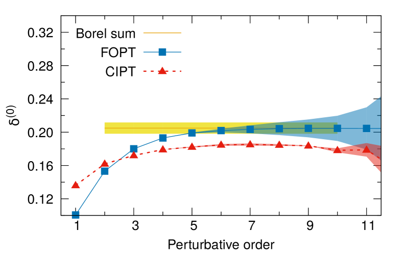
Figure 8: Final results for $\delta^{(0)}$ in QCD using the coefficients of Tab. 6 and the result of Eq. (47). The bands in the perturbative expansions reflect the uncertainty in the coefficients while the band in the sum of the series is obtained from the spread of the values from individual PAs (last columns of Tabs. 4 and 5). We use $\alpha_{s}(m_{\tau}^{2})=0.316.$

With the coefficients of Tab. 6 we are finally in a position to plot, in Fig. 8, the perturbative expansions of $\delta^{(0)}$ and compare them with the true value of the series obtained from Eq. (47). The bands in the perturbative expansions of Fig. 8 represent the uncertainty from the series coefficients, given in Tab. 6, while the band in the Borel sum of the series is the first error Eq. (47). The uncertainties we are able to obtain from the optimal Padé approximants allow us to conclude that FOPT is the favored renormalization-scale setting procedure in the case of full QCD. The CIPT series, even though it looks more stable around the fourth order, does not approach well the central value of the sum of the series. The recommendation that FOPT is the best procedure in QCD was advocated in Ref. [18] in the renormalon-model context. Here it is reobtained in a model-independent way.

6 Conclusions

In this work we have performed a systematic study of the Adler function and of the perturbative QCD correction to the hadronic $\tau$ decay width, $\delta^{(0)}$, using Padé approximants and its variants. We have used the large-$\beta_{0}$ limit of QCD, where the series are known to all orders in $\alpha_{s}$, as a laboratory to test our strategy. We were able to show that the method always works provided a large enough number of coefficients is known. Since in QCD only the first four have been calculated exactly, we have devised strategies with the aim of accelerating the convergence of the approximants. The success of these strategies can be understood in terms of the analytic structure of the Borel transformed series. The model independent acceleration methods simplify this structure either by suppressing the residue of some poles or by reducing their multiplicity.

A similar suppression of the poles is also found in the Borel transform of $\delta^{(0)}$ which automatically leads to a more regular series that is more amenable to approximation by PAs. We have exploited this fact to show that, in large-$\beta_{0}$, the PAs formed to the $\alpha_{s}$ expansion of $\delta^{(0)}$ and the D-log PAs constructed to its Borel transform $B[\delta^{(0)}]$ are the optimal model-independent way of extracting the higher-order coefficients of the Adler function.

We have then applied the same procedure to full QCD. The excellent “postdiction” of the coefficient $c_{4,1}$, which is known since 2008 [21], as well as the striking stability of the results gives us confidence that the method also works in QCD. From PAs to the fixed-order expansion of $\delta^{(0)}$ and D-log PAs to $B[\delta^{(0)}]$ we extract the final results of this paper, given in Tab. 6 and Eq. (47). These results allow us to reconstruct very reliably the perturbative expansions of $\delta^{(0)}$ up to at least the tenth order. Finally, Fig. 8 shows that our model-independent reconstruction of the higher-order series coefficients favours FOPT as the best procedure to set the renormalization scale at and around the $\tau$ mass.

We should remark that our final results are similar to the model-dependent reconstruction of the series put forward in Ref. [18] and further discussed in Ref. [25]. This lends support to renormalon model used in these works, even though the use of PAs show that one should be careful when interpreting the parameters of such models. In the case of the renormalon models, the analytic structure is completely fixed, the only freedom is left to the residues. Therefore, we should expect that these are “effective residues”, in the spirit of Padé-type approximants, and can only be compared with the true residues in a hierarchical way, since they must account for the infinite tower of poles that must be mimicked by the model.

Apart from providing reliable estimates for the higher-orders coefficients and indicating that FOPT is preferred, our results could be the basis for an $\alpha_{s}$ extraction based on the Borel sum of $\delta^{(0)}$. The fact that the results of Eqs. (47–51) are so close suggest that it may be realistic to do so. We also intend to investigate further the analytic structure of $B[\delta^{(0)}]$ in QCD, since the non-trivial result of Eq. (23) plays a central role in our analysis. The simplicity and flexibility of the method here developed suggests it could also be used to further explore non-perturbative contributions in the context of $\alpha_{s}$ determinations.

References

- [1] G. Degrassi, S. Di Vita, J. Elias-Miró, J. R. Espinosa, G. F. Giudice, G. Isidori and A. Strumia, Higgs mass and vacuum stability in the Standard Model at NNLO, JHEP 1208, 098 (2012), [arXiv:1205.6497 [hep-ph]].
- [2] E. Braaten, S. Narison and A. Pich, QCD analysis of the tau hadronic width, Nucl. Phys. B 373, 581 (1992).
- [3] D. Boito, M. Golterman, K. Maltman, J. Osborne and S. Peris, Strong coupling from the revised ALEPH data for hadronic decays, Phys. Rev. D 91, no. 3, 034003 (2015), [arXiv:1410.3528 [hep-ph]].
- [4] A. Pich and A. Rodríguez-Sánchez, Determination of the QCD coupling from ALEPH decay data, Phys. Rev. D 94, no. 3, 034027 (2016), [arXiv:1605.06830 [hep-ph]].
- [5] M. Davier, A. Höcker, B. Malaescu, C. Z. Yuan and Z. Zhang, Update of the ALEPH non-strange spectral functions from hadronic decays, Eur. Phys. J. C 74, no. 3, 2803 (2014), [arXiv:1312.1501 [hep-ex]].
- [6] A. Keshavarzi, D. Nomura and T. Teubner, The muon and : a new data-based analysis, Phys. Rev. D 97, no. 11, 114025 (2018) [arXiv:1802.02995 [hep-ph]].
- [7] D. Boito, M. Golterman, A. Keshavarzi, K. Maltman, D. Nomura, S. Peris and T. Teubner, The strong coupling from hadrons below charm, arXiv:1805.08176 [hep-ph].
- [8] A. Pich, Precision Tau Physics, Prog. Part. Nucl. Phys. 75, 41 (2014), [arXiv:1310.7922 [hep-ph]].
- [9] T. van Ritbergen, J. A. M. Vermaseren and S. A. Larin, The Four loop beta function in quantum chromodynamics, Phys. Lett. B 400, 379 (1997), [hep-ph/9701390].
- [10] P. A. Baikov, K. G. Chetyrkin and J. H. Kühn, Five-Loop Running of the QCD coupling constant, Phys. Rev. Lett. 118, no. 8, 082002 (2017), [arXiv:1606.08659 [hep-ph]].
- [11] F. Herzog, B. Ruijl, T. Ueda, J. A. M. Vermaseren and A. Vogt, The five-loop beta function of Yang-Mills theory with fermions, JHEP 1702, 090 (2017), [arXiv:1701.01404 [hep-ph]].
- [12] T. Luthe, A. Maier, P. Marquard and Y. Schroder, The five-loop Beta function for a general gauge group and anomalous dimensions beyond Feynman gauge, JHEP 1710, 166 (2017), [arXiv:1709.07718 [hep-ph]].
- [13] D. Boito, M. Golterman, K. Maltman and S. Peris, Strong coupling from hadronic decays: A critical appraisal, Phys. Rev. D 95, no. 3, 034024 (2017), [arXiv:1611.03457 [hep-ph]].
- [14] M. A. Shifman, Quark hadron duality, In *Shifman, M. (ed.): At the frontier of particle physics, vol. 3* 1447-1494 [hep-ph/0009131].
- [15] O. Catà, M. Golterman and S. Peris, Duality violations and spectral sum rules, JHEP 0508, 076 (2005), [hep-ph/0506004].
- [16] S. Peris, D. Boito, M. Golterman and K. Maltman, The case for duality violations in the analysis of hadronic decays, Mod. Phys. Lett. A 31, no. 30, 1630031 (2016), [arXiv:1606.08898 [hep-ph]].
- [17] D. Boito, I. Caprini, M. Golterman, K. Maltman and S. Peris, Hyperasymptotics and quark-hadron duality violations in QCD, Phys. Rev. D 97, no. 5, 054007 (2018), [arXiv:1711.10316 [hep-ph]].
- [18] M. Beneke and M. Jamin, and the hadronic width: fixed-order, contour-improved and higher-order perturbation theory, JHEP 0809, 044 (2008), [arXiv:0806.3156 [hep-ph]].
- [19] F. Le Diberder and A. Pich, Testing QCD with decays, Phys. Lett. B 289, 165 (1992).
- [20] A. A. Pivovarov, Renormalization group analysis of the tau lepton decay within QCD, Z. Phys. C 53, 461 (1992), Sov. J. Nucl. Phys. 54, 676 (1991) Yad. Fiz. 54, 1114 (1991), [hep-ph/0302003].
- [21] P. A. Baikov, K. G. Chetyrkin and J. H. Kühn, Order QCD corrections to Z and decays, Phys. Rev. Lett. 101, 012002 (2008), [arXiv:0801.1821 [hep-ph]].
- [22] F. Herzog, B. Ruijl, T. Ueda, J. A. M. Vermaseren and A. Vogt, On Higgs decays to hadrons and the R-ratio at N4LO, JHEP 1708, 113 (2017), [arXiv:1707.01044 [hep-ph]].
- [23] J. Kühn, private communication.
- [24] M. Beneke, Renormalons, Phys. Rept. 317, 1 (1999), [hep-ph/9807443].
- [25] M. Beneke, D. Boito and M. Jamin, Perturbative expansion of hadronic spectral function moments and extractions, JHEP 1301, 125 (2013), [arXiv:1210.8038 [hep-ph]].
- [26] G. A. Baker, Essentials of Padé Approximants, Academic Press (1975). G. A. Baker and P. Graves-Morris, Encyclopedia of Mathematics and Its Applications (Cambridge University Press, Cambridge, England, 1996). For a brief overview, see C. Bender and S. Orszag,Advanced Mathematical Methods for Scientists and Engineers I: asymptotic methods and perturbation theory. Springer 1999, section 8.6.
- [27] P. Masjuan and S. Peris, A Rational approach to resonance saturation in large-N(c) QCD, JHEP 0705, 040 (2007), [arXiv:0704.1247 [hep-ph]].
- [28] P. Masjuan and S. Peris, A Rational approximation to and its O() low-energy constant, Phys. Lett. B 663 (2008) 61, [arXiv:0801.3558 [hep-ph]].
- [29] P. Masjuan and S. Peris, Padé Theory applied to the vacuum polarization of a heavy quark, Phys. Lett. B 686 (2010) 307, [arXiv:0903.0294 [hep-ph]].
- [30] M. A. Samuel, J. R. Ellis and M. Karliner, Comparison of the Padé approximation method to perturbative QCD calculations, Phys. Rev. Lett. 74, 4380 (1995), [hep-ph/9503411].
- [31] G. A. Baker, B. G. Nickel, M. S. Green and D. I. Meiron, Ising Model Critical Indices in Three-Dimensions from the Callan-Symanzik Equation, Phys. Rev. Lett. 36, 1351 (1976).
- [32] J. R. Ellis, E. Gardi, M. Karliner and M. A. Samuel, Padé approximants, Borel transforms and renormalons: The Bjorken sum rule as a case study, Phys. Lett. B 366, 268 (1996), [hep-ph/9509312].
- [33] M. Beneke, Large order perturbation theory for a physical quantity, Nucl. Phys. B 405, 424 (1993).
- [34] D. J. Broadhurst, Large N expansion of QED: Asymptotic photon propagator and contributions to the muon anomaly, for any number of loops, Z. Phys. C 58, 339 (1993).
- [35] Ch. Pommerenke, J. Math. Anal. Appl. 41 775 (1973).
- [36] D. Boito, M. Jamin and R. Miravitllas, Scheme Variations of the QCD Coupling and Hadronic Decays, Phys. Rev. Lett. 117, no. 15, 152001 (2016), [arXiv:1606.06175 [hep-ph]].
- [37] M. Jamin and R. Miravitllas, Scalar correlator, Higgs decay into quarks, and scheme variations of the QCD coupling, JHEP 1610, 059 (2016), [arXiv:1606.06166 [hep-ph]].
- [38] L. S. Brown and L. G. Yaffe, Asymptotic behavior of perturbation theory for the electromagnetic current current correlation function in QCD, Phys. Rev. D 45, 398 (1992); L. S. Brown, L. G. Yaffe and C. X. Zhai, Large order perturbation theory for the electromagnetic current current correlation function, Phys. Rev. D 46, 4712 (1992), [hep-ph/9205213].
- [39] D. Boito and F. Oliani, in preparation.
- [40] D. Boito, O. Catà, M. Golterman, M. Jamin, K. Maltman, J. Osborne and S. Peris, A new determination of from hadronic decays, Phys. Rev. D 84, 113006 (2011), [arXiv:1110.1127 [hep-ph]].
- [41] M. Jamin, Contour-improved versus fixed-order perturbation theory in hadronic decays, JHEP 0509, 058 (2005), [hep-ph/0509001].
- [42] I. Caprini and J. Fischer, Expansion functions in perturbative QCD and the determination of , Phys. Rev. D 84, 054019 (2011), [arXiv:1106.5336 [hep-ph]].
- [43] G. Abbas, B. Ananthanarayan and I. Caprini, Determination of from Improved Fixed Order Perturbation Theory, Phys. Rev. D 85, 094018 (2012) [arXiv:1202.2672 [hep-ph]].
- [44] G. Abbas, B. Ananthanarayan, I. Caprini and J. Fischer, Perturbative expansion of the QCD Adler function improved by renormalization-group summation and analytic continuation in the Borel plane, Phys. Rev. D 87, no. 1, 014008 (2013), [arXiv:1211.4316 [hep-ph]]; Expansions of hadronic spectral function moments in a nonpower QCD perturbation theory with tamed large order behavior,” Phys. Rev. D 88, no. 3, 034026 (2013) [arXiv:1307.6323 [hep-ph]].
- [45] I. Caprini, J. Fischer, G. Abbas and B. Ananthanarayan, Perturbative Expansions in QCD Improved by Conformal Mappings of the Borel Plane, [arXiv:1711.04445 [hep-ph]].
- [46] G. Cvetic, M. Loewe, C. Martinez and C. Valenzuela, Modified Contour-Improved Perturbation Theory, Phys. Rev. D 82, 093007 (2010), [arXiv:1005.4444 [hep-ph]].
- [47] D. Boito, M. Jamin and R. Miravitllas, Scheme variations of the QCD coupling and decays, Nucl. Part. Phys. Proc. 287-288, 77 (2017), [arXiv:1612.05558 [hep-ph]].
- [48] C. Díaz-Mendoza, P. González-Vera, and R. Orive, On the convergence of two-point partial Padé approximants for meromorphic functions of Stieltjes type, Appl. Num. Math. 53 29 (2005).
- [49] C. Patrignani et al. [Particle Data Group], Review of Particle Physics, Chin. Phys. C 40, no. 10, 100001 (2016).
- [50] D. Boito, M. Jamin and R. Miravitllas, Scheme variations of the QCD coupling, EPJ Web Conf. 137, 05007 (2017) [arXiv:1612.01792 [hep-ph]].
- [51] W. Celmaster and R. J. Gonsalves, The Renormalization Prescription Dependence of the QCD Coupling Constant, Phys. Rev. D 20, 1420 (1979).
- [52] P. A. Baikov, K. G. Chetyrkin and J. H. Kühn, Towards order accuracy in tau decays, Phys. Rev. D 67, 074026 (2003) [hep-ph/0212299].
- [53] A. L. Kataev and V. V. Starshenko, Estimates of the higher order QCD corrections: Theory and applications, Nucl. Phys. Proc. Suppl. 39BC, 312 (1995) [hep-ph/9408395].
- [54] A. L. Kataev and V. V. Starshenko, Estimates of the higher order QCD corrections to R(s), R(tau) and deep inelastic scattering sum rules, Mod. Phys. Lett. A 10, 235 (1995), [hep-ph/9502348].
- [55] D. Boito, D. Hornung and M. Jamin, Anomalous dimensions of four-quark operators and renormalon structure of mesonic two-point correlators, JHEP 1512, 090 (2015) [arXiv:1510.03812 [hep-ph]].
- [56] X. G. Wu, J. M. Shen, B. L. Du and S. J. Brodsky, Novel demonstration of the renormalization group invariance of the fixed-order predictions using the principle of maximum conformality and the -scheme coupling, Phys. Rev. D 97, no. 9, 094030 (2018) [arXiv:1802.09154 [hep-ph]].
- [57] I. Caprini, Renormalization-scheme variation of a QCD perturbation expansion with tamed large-order behaviour, arXiv:1806.10325 [hep-ph].