On the zero set of the partial theta function

Abstract.

We consider the partial theta function $\theta(q,x):=\sum_{j=0}^{\infty}q^{j(j+1)/2}x^{j}$, where $q\in(-1,0)\cup(0,1)$ and either $x\in\mathbb{R}$ or $x\in\mathbb{C}$. We prove that for $x\in\mathbb{R}$, in each of the two cases $q\in(-1,0)$ and $q\in(0,1)$, its zero set consists of countably-many smooth curves in the $(q,x)$-plane each of which (with the exception of one curve for $q\in(-1,0)$) has a single point with a tangent line parallel to the $x$-axis. These points define double zeros of the function $\theta(q,.)$; their $x$-coordinates belong to the interval $[-38.83\ldots,-e^{1.4}=4.05\ldots)$ for $q\in(0,1)$ and to the interval $(-13.29,23.65)$ for $q\in(-1,0)$. For $q\in(0,1)$, infinitely-many of the complex conjugate pairs of zeros to which the double zeros give rise cross the imaginary axis and then remain in the half-disk $\{|x|<18$, Re $x>0\}$. For $q\in(-1,0)$, complex conjugate pairs do not cross the imaginary axis.

Key words: partial theta function, Jacobi theta function, Jacobi triple product

AMS classification: 26A06

1. Introduction

We consider the bivariate series $\theta(q,x):=\sum_{j=0}^{\infty}q^{j(j+1)/2}x^{j}$ which converges for $q\in(-1,1)$, $x\in\mathbb{C}$, and defines (for each fixed value of the parameter $q$) an entire function in $x$. We refer to $\theta$ as to a partial theta function. The terminology is justified by the fact that the series $\Theta(q,x):=\sum_{j=-\infty}^{\infty}q^{j^{2}}x^{j}$ defines the Jacobi theta function, and one has $\theta(q^{2},x/q)=\sum_{j=0}^{\infty}q^{j^{2}}x^{j}$. The word “partial” hints at the fact that summation in $\theta$ is only partial (not from $-\infty$ to $\infty$, but only from $0$ to $\infty$). The function $\theta$ satisfies the differential equation

(1.1) $$2q\partial\theta/\partial q=x(\partial^{2}/\partial x^{2})(x\theta)=x^{2}\partial^{2}\theta/\partial x^{2}+2x\partial\theta/\partial x$$

and the functional equation

(1.2) $$\theta(q,x)=1+qx\theta(q,qx)~{}.$$

The interest in the function $\theta$ is explained by its applications in different areas. One of the most recent of them is about section-hyperbolic polynomials, i.e. real polynomials in one variable of degree $\geq 2$ having only real negative roots and such that when one deletes their highest-degree monomial, one obtains again a polynomial with all roots real negative. How $\theta$ arises in the context of such polynomials is explained in [18]. The explanation uses the notion of the spectrum of $\theta$ (see Section 2). The research on section-hyperbolic polynomials continued the activity in this domain which was marked by papers [8] and [19], and which were inspired by earlier results of Hardy, Petrovitch and Hutchinson (see [6], [20] and [7]). Section-hyperbolic polynomials are real, therefore the case when the parameter $q$ is real is of particular interest. The case $q\in\mathbb{C}$, $|q|<1$ (which has been studied by the author in [14], [13] and [12]) is not considered in the present paper.

The partial theta function is used in other domains as well. Such are asymptotic analysis (see [2]), statistical physics and combinatorics (see [22]), Ramanujan-type $q$-series (see [23]) and the theory of (mock) modular forms (see [4]); see also [1]. Recently, new asymptotic results for Jacobi partial and false theta functions have been proved in [3]. They originate from Jacobi forms and find applications when considering the asymptotic expansions of regularized characters and quantum dimensions of the $(1,p)$-singlet algebra modules. The article [5] is a closely related paper dealing with modularity, asymptotics and other properties of partial and false theta functions which are treated in the framework of conformal field theory and representation theory.

The present paper studies properties of the zero set of $\theta$. The case $q=0$ being trivial (with $\theta(0,x)\equiv 1$) one has to study in fact two different cases, namely $q\in(0,1)$ and $q\in(-1,0)$, in which the results are formulated in different ways. We present three different kinds of results. In Section 2 we describe the set of real zeros of $\theta$ as a union of smooth curves in the $(q,x)$-space, see Theorem 3. These results are further developed in Section 4 by means of properties of certain functions in one variable; these properties are proved in Section 3.

It is known that for each $q\in(-1,0)\cup(0,1)$ fixed, $\theta(q,.)$ has either only simple zeros or simple zeros and one double zero, see Theorems 1 and 2. In Section 5 we prove that for $q\in(0,1)$, all double zeros of $\theta$ belong to the interval $[-38.83960007\ldots,-4.055199967\ldots)$ (Theorem 5); for $q\in(-1,0)$, they belong to the interval $(-13.29,23.65)$ (Theorem 6). In Section 6 we describe the behaviour of the complex conjugate pairs of $\theta(q,.)$. We show in Subsection 6.1 that in the case $q\in(-1,0)$, complex conjugate pairs do not cross the imaginary axis (Theorem 7); hence each zero of $\theta$ remains in the left or right half-plane for all $q\in(-1,0)$. In Subsection 6.2 we show that as $q$ increases in $(0,1)$, infinitely-many complex conjugate pairs of $\theta$ go to the right half-plane, and after this remain in the half-disk $\{|x|<18$, Re $x>0\}$.

2. Geometry of the zero set of $\theta$

First of all, we recall some known results in the case $q\in(0,1)$ (see [9]):

Theorem 1.

(1) For $q\in(0,\tilde{q}_{1}:=0.3092\ldots)$, all zeros of $\theta(q,.)$ are real, negative and distinct: $\cdots<\xi_{2}<\xi_{1}<0$.

(2) There exist countably-many values $0<\tilde{q}_{1}<\tilde{q}_{2}<\cdots<1$ of $q$, where $\tilde{q}_{j}\rightarrow 1^{-}$ as $j\rightarrow\infty$, for which $\theta(q,.)$ has a multiple real zero $y_{j}$. For any $j\in\mathbb{N}$, this is the rightmost of the real zeros of $\theta$; it is a double zero of $\theta$.

(3) For $q\in(\tilde{q}_{j},\tilde{q}_{j+1})$ (we set $\tilde{q}_{0}:=0$), the function $\theta(q,.)$ has exactly $j$ complex conjugate pairs of zeros (counted with multiplicity).

Definition 1.

We call spectrum of $\theta$ the set of values of $q$ for which $\theta(q,.)$ has at least one multiple zero. This notion is introduced by B. Z. Shapiro in [18].

Remarks 1.

(1) The zeros of $\theta$ depend continuously on $q$. Due to this, for $q\in(0,\tilde{q}_{j})$, the order of its zeros $\cdots<\xi_{2j}<\xi_{2j-1}<0$ on the real line is well-defined. For no $q\in(0,1)$ does $\theta(q,.)$ have a nonnegative zero. For $q=\tilde{q}_{j}$, the zeros $\xi_{2j-1}$ and $\xi_{2j}$ coalesce and then become a complex conjugate pair for $q=(\tilde{q}_{j})^{+}$; thus the indices $2j-1$ and $2j$ of the real zeros are meaningful exactly when $q\in(0,\tilde{q}_{j}]$. For $q\in(\tilde{q}_{j},\tilde{q}_{j+1})$, one has

$$\left\{\begin{array}[]{lll}\theta(q,x)>0&{\rm for}&x\in(\xi_{2j+1},\infty)\cup(\cup_{k=j+1}^{\infty}(\xi_{2k+1},\xi_{2k}))\\ \\ \theta(q,x)<0&{\rm for}&x\in(\cup_{k=j+1}^{\infty}(\xi_{2k},\xi_{2k-1})~{}.\end{array}\right.$$

(2) In the above setting, one has $-q^{-2j-2}<\xi_{2j+2}<\xi_{2j+1}<-q^{-2j-1}$, see Proposition 9 in [9].

(3) The function $\theta(\tilde{q}_{j},.)$ has a local minimum at its double zero $y_{j}$. One has $\tilde{q}_{j}=1-\pi/2j+o(1/j)$ and $y_{j}=-e^{\pi}+o(1)$, where $e^{\pi}=23.14\ldots$, see [16] or [10]. Up to the sixth decimal, the first six spectral values $\tilde{q}_{j}$ equal $0.309249$, $0.516959$, $0.630628$, $0.701265$, $0.749269$, $0.783984$, see [18].

The analog of Theorem 1 in the case $q\in(-1,0)$ reads (see [15]):

Theorem 2.

(1) For any $q\in(-1,0)$, the function $\theta(q,.)$ has infinitely-many negative and infinitely-many positive zeros.

(2) There exists a sequence of values $\bar{q}_{j}$ of $q$ tending to $-1^{+}$ for which the function $\theta(\bar{q}_{j},.)$ has a double real zero $\bar{y}_{j}$ (the rest of its real zeros being simple). For the rest of the values of $q\in(-1,0)$, $\theta(q,.)$ has no multiple real zeros. For $j$ large enough, one has $-1<\bar{q}_{j+1}<\bar{q}_{j}<0$.

(3) For $j$ odd, one has $\bar{y}_{j}<0$, $\theta(\bar{q}_{j},.)$ has a local minimum at $\bar{y}_{j}$ and $\bar{y}_{j}$ is the rightmost of the negative zeros of $\theta(\bar{q}_{j},.)$. For $j$ even, one has $\bar{y}_{j}>0$, $\theta(\bar{q}_{j},.)$ has a local maximum at $\bar{y}_{j}$ and $\bar{y}_{j}$ is the second from the left of the positive zeros of $\theta(\bar{q}_{j},.)$.

(4) For $j$ sufficiently large and for $q\in(\bar{q}_{j+1},\bar{q}_{j})$, the function $\theta(q,.)$ has exactly $j$ complex conjugate pairs of zeros counted with multiplicity.

For $q\in(-1,0)$, the first six spectral values $\bar{q}_{j}$ equal (up to the sixth decimal) $-0.727133$, $-0.783742$, $-0.841601$, $-0.861257$, $-0.887952$ and $-0.897904$, see [15].

Remark 1.

For $q\in(-1,0)$ sufficiently close to $0$, all zeros of $\theta(q,.)$ are real. We denote them by $\cdots<\zeta_{2}<\zeta_{1}<0$ and $0<\eta_{1}<\eta_{2}<\cdots$. For $j=2\nu-1$ (resp. for $j=2\nu$), $\nu\in\mathbb{N}$, the zeros $\zeta_{2\nu-1}$ and $\zeta_{2\nu}$ (resp. $\eta_{2\nu}$ and $\eta_{2\nu+1}$) coalesce at $\bar{y}_{2\nu-1}$ when $q=\bar{q}_{2\nu-1}$ (resp. at $\bar{y}_{2\nu}$ when $q=\bar{q}_{2\nu}$). Thus the zero $\eta_{1}$ remains real positive and simple for all $q\in(-1,0)$. This is deduced in [15], from the order of the quantities $\zeta_{j}$, $q\zeta_{j}$, $\eta_{k}$ and $q\eta_{k}$ on the real line (see Fig. 3 in [15]; the notation used in [15] is not the one we use here):

$$\begin{array}[]{ccccccccccccccccc}\cdots&<&\zeta_{4}&<&\zeta_{3}&<&q\eta_{4}&<&q\eta_{3}&<&\zeta_{2}&<&\zeta_{1}&<&q\eta_{2}&<&0\\ \\ 0&<&\eta_{1}&<&q\zeta_{1}&<&q\zeta_{2}&<&\eta_{2}&<&\eta_{3}&<&q\zeta_{3}&<&q\zeta_{4}&<&\cdots~{}~{}.\end{array}$$

Our first result is formulated as follows:

Theorem 3.

(1) Suppose that $q\in(0,1)$. For $j=1$, $2$, $\ldots$, consider the zeros $\xi_{2j-1}$ and $\xi_{2j}$ as functions in $q\in(0,\tilde{q}_{j}]$. Their two graphs together (in the $(q,x)$-plane) form a smooth curve $\Gamma_{j}$ having two parabolic branches $B_{2j-1}$ and $B_{2j}$ which are asymptotically equivalent to $x=-q^{-2j+1}$ and $x=-q^{-2j}$ as $q\rightarrow 0^{+}$. The curve $\Gamma_{j}$ has a single point $X_{j}$, namely for $q=\tilde{q}_{j}$, at which the tangent line is parallel to the $x$-axis.

(2) Suppose that $q\in(-1,0)$. For $\nu=1$, $2$, $\ldots$, consider the zeros $\zeta_{2\nu-1}$ and $\zeta_{2\nu}$ (resp. $\eta_{2\nu}$ and $\eta_{2\nu+1}$) as functions in $q\in[\bar{q}_{2\nu-1},0)$ (resp. $q\in[\bar{q}_{2\nu},0)$). Their two graphs together (in the $(q,x)$-plane) form a smooth curve $\Gamma_{\nu}^{-}$ (resp. $\Gamma_{\nu}^{+}$) having two parabolic branches $B_{2\nu-1}^{-}$ and $B_{2\nu}^{-}$ (resp. $B_{2\nu}^{+}$ and $B_{2\nu+1}^{+}$) which are asymptotically equivalent to $x=-q^{-4\nu+2}$ and $x=-q^{-4\nu}$ (resp. $x=-q^{-4\nu+1}$ and $x=-q^{-4\nu-1}$) as $q\rightarrow 0^{-}$. The curve $\Gamma_{\nu}^{-}$ (resp. $\Gamma_{\nu}^{+}$) has a single point $X_{\nu}^{-}$ (resp. $X_{\nu}^{+}$) such that for $q=\bar{q}_{2\nu-1}$ (resp. for $q=\bar{q}_{2\nu}$), the tangent line to $\Gamma_{\nu}^{-}$ at $X_{\nu}^{-}$ (resp. to $\Gamma_{\nu}^{+}$ at $X_{\nu}^{+}$) is parallel to the $x$-axis. The graph of the zero $\eta_{1}$ is asymptotically equivalent to $-q^{-1}$ as $q\rightarrow 0^{-}$ and one has $\eta_{1}\rightarrow 1^{+}$ as $q\rightarrow-1^{+}$.

Remarks 2.

(1) It is clear that the function $\xi_{2j-1}$ cannot be everywhere increasing on $(0,\tilde{q}_{j}]$ – for $q$ close to $\tilde{q}_{j}$, the slope of the tangent line to its graph is positive whereas for $q$ close to $0$, it is negative. The graphs of the zeros $\xi_{2j-1}$ and $\xi_{2j}$ which coalesce for $q=\tilde{q}_{j}$ can be compared with the graphs of $\pm\sqrt{q}$ at $0$. Similar remarks can be made about the zeros $\zeta_{j}$ and $\eta_{j}$.

(2) The curves $x=-q^{-s}$ can be considered as curvilinear asymptotes to the zero set of $\theta$.

Conjecture 1.

The curve $\Gamma_{j}$ from Theorem 3 has a single point $Q_{j}$ at which the tangent line is parallel to the $q$-axis, a single inflection point $I_{j}$ and a single point $D_{j}\in\Gamma_{j}$ at which one has $\theta(q,-q^{-2s+1/2})=0$. The order of the points and branches of $\Gamma_{j}$ is the following one: $B_{2j-1}$, $Q_{j}$, $D_{j}$, $X_{j}$, $I_{j}$, $B_{2j}$. The function $\xi_{2j}$ is everywhere increasing on $(0,\tilde{q}_{j}]$.

On Fig. 1 we show parts of the curves $\Gamma_{1}$, $\Gamma_{2}$ and $\Gamma_{3}$ (drawn in solid line) and of the graphs of the functions $x=-q^{a}$ for $a=0.5$, $-1.5$ (drawn in solid), $-2.5$, $-3,5$ (drawn in dashed), $-1$ and $-2$ (drawn in dotted line). On Fig. 1 we show also the horizontal dash-dotted lines $q=0.26$ and $q=0.4$. We say that the part of the curve $x=-q^{-1.5}$ corresponding to $q\in(0,0.26]$ is inside and the part corresponding to $q\in[0.4,1)$ is outside the curve $\Gamma_{1}$.

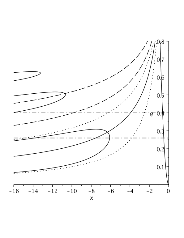
Figure 1. The curves $\Gamma_{1}$, $\Gamma_{2}$ and $\Gamma_{3}$ and the graphs $x=-q^{a}$ for $a=0.5$, $-1.5$, $-2.5$, $-3,5$, $-1$ and $-2$.

On Fig. 2 we show for $q\in(-1,0)$ the real-zero set of $\theta$ (in solid line) and the curves $x=-q^{-a}$, $a=1$, $\ldots$, $8$ (in dashed line for $a=1$, $2$, $5$ and $6$, and in dotted line for $a=3$, $4$, $7$ and $8$).

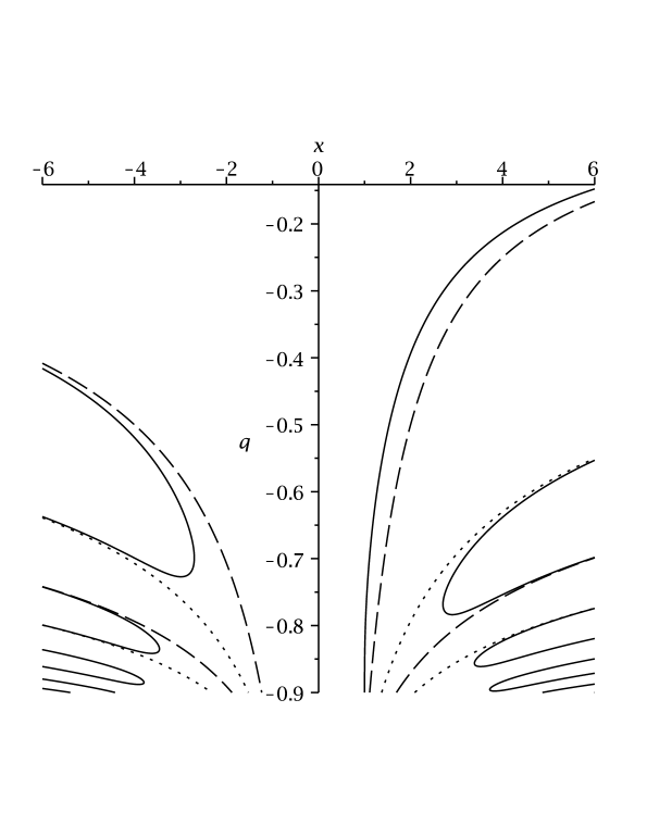
Figure 2. The zero set of $\theta$ for $q\in(-1,0)$ and the curves $x=-q^{-a}$ for $a=1$, $\ldots$, $8$.

Remarks 3.

(1) Suppose that $q\in(0,1)$. Inside (resp. outside) each curve $\Gamma_{j}$ one has $\theta(q,x)<0$ (resp. $\theta(q,x)>0$).

(2) One can check numerically that $\Gamma_{1}\subset\{x\leq-6.095\}$. One can conjecture that any real zero of $\theta(q,.)$, for any $q\in(0,1)$, is smaller than $-6.095$.

(3) Suppose that $q\in(-1,0)$. Inside each curve $\Gamma_{\nu}^{-}$ (resp. $\Gamma_{\nu}^{+}$) one has $\theta(q,x)<0$ (resp. $\theta(q,x)>0$). For $x<\eta_{1}$ (resp. $x>\eta_{1}$) and $(q,x)$ outside the curves $\Gamma_{\nu}^{-}$ (resp. $\Gamma_{\nu}^{+}$) one has $\theta(q,x)>0$ (resp. $\theta(q,x)<0$).

(4) One can check numerically that $\Gamma_{1}^{-}\subset\{x\leq-2.699\}$. One can conjecture that any negative real zero of $\theta(q,.)$, for any $q\in(-1,0)$, is smaller than $-2.699$.

(5) For any $q\in(-1,0)$, the function $\theta(q,.)$ has no real zero in the interval $[-1,1]$. Indeed, one has $\theta(q,0)=1\neq 0$. For $x\in(0,\eta_{1})$, one has $\theta(q,x)>0$, see part (3) of these remarks. For $x\in[-1,0)$, one obtains $\theta(q,x)=1+qx\theta(q,qx)$, where $qx\in(0,1)$ hence $qx\theta(q,qx)>0$ and $\theta(q,x)>0$.

Proof of Theorem 3:.

Part (1). The claims about the branches $B_{2j-1}$ and $B_{2j}$ follow from Theorem 4 in [9]; for the branches $B_{\nu}^{\pm}$ this follows from part (1) of Theorem 1 in [11]. Smoothness of $\Gamma_{j}$ has to be proved only at $X_{j}$, everywhere else $\Gamma_{j}$ is the graph of a simple zero of $\theta$ which depends smoothly on $q$. For $q=\tilde{q}_{j}$, the function $\theta$ has a double zero at $\xi_{2j-1}=\xi_{2j}$, so $(\partial\theta/\partial x)(\tilde{q}_{j},\xi_{2j-1})=0$ and $(\partial^{2}\theta/\partial x^{2})(\tilde{q}_{j},\xi_{2j-1})\neq 0$. This implies $(\partial\theta/\partial q)(\tilde{q}_{j},\xi_{2j-1})\neq 0$, see (1.1), from which smoothness of $\Gamma_{j}$ at $X_{j}$ follows. Simplicity of the zeros $\xi_{2j-1}$ and $\xi_{2j}$ for $q\in(0,\tilde{q}_{j})$ excludes tangents parallel to the $x$-axis on $\Gamma_{j}\backslash\{X_{j}\}$.

Part (2). The claims about the curves $\Gamma_{j}^{\pm}$ are proved by analogy with the claims about the curves $\Gamma_{j}$. By Proposition 4.5 of [15], one has $\theta(q,-q^{-1})<0$. (On Fig. 2 this corresponds to the fact that the graph of $\eta_{1}$ is to the left of the dashed curve $x=-q^{-1}$.) We show that $\theta(q,1)>0$ from which follows that $\eta_{1}\rightarrow 1^{+}$ as $q\rightarrow-1^{+}$. For $|q|<1$, one has

$$\theta(q,1)=\sum_{j=0}^{\infty}q^{j(j+1)/2}=\frac{1-q^{2}}{1-q}\cdot\frac{1-q^{4}}{1-q^{3}}\cdot\frac{1-q^{6}}{1-q^{5}}\cdots~{},$$

see Problem 55 in Part I, Chapter 1 of [21]. For $q\in(-1,0)$, all factors in the right-hand side are positive, hence $\theta(q,1)>0$. ∎

3. The functions $\varphi_{k}$

In the present section we consider some functions in one variable which play an important role in the proofs in this paper:

(3.3) $$\varphi_{k}(q):=\theta(q,-q^{k-1})=\sum_{j=0}^{\infty}(-1)^{j}q^{A_{j}}~{},~{}~{}~{}A_{j}:=kj+j(j-1)/2~{},~{}~{}~{}k\in\mathbb{R}~{}.$$

In the notation for $A_{j}$ we skip the parameter $k$ in order not to have too many indices. We prove the following theorem:

Theorem 4.

(1) For $k>1$, the function $\varphi_{k}$ is of the class $C^{1}_{(0,1)}\cap C_{[0,1]}$; its right derivative at $0$ exists and equals $0$. For $k>0$, its left derivative at $1$ exists and equals $-(2k-1)/8$.

(2) For $k>0$ sufficiently large, the function $\varphi_{k}$ is decreasing on $[0,1]$.

We prove part (1) of the theorem after the formulations of Propositions 1 and 2, and part (2) at the end of the section.

Remarks 4.

(1) The functions $\varphi_{k}$ satisfy the functional equation

(3.4) $$\varphi_{k}=1-q\varphi_{k+1}~{}.$$

One can deduce from this equation that the formula for the left derivative at $1$ remains valid for all $k\in\mathbb{R}$. For $k\in\mathbb{Z}$, the function $\varphi_{k}$ belongs to the class $C^{1}_{(0,1)}\cap C_{[0,1]}$ (the negative powers of $q$ cancel). For $k<0$, $k\not\in\mathbb{Z}$, one has $\varphi_{k}(q)\rightarrow\infty$ or $\varphi_{k}(q)\rightarrow-\infty$ as $q\rightarrow 0^{+}$ depending on the parity of $[k]$ (the integer part of $k$).

(2) We remind that:

i) For $k>0$ (resp. for $k>1$) and $q\in(0,1)$, one has $\varphi_{k}<1/(1+q^{k})$ (resp. $1/(1+q^{k-1})<\varphi_{k}$), and that $\lim_{q\rightarrow 1^{-}}\varphi_{k}(q)=1/2$, see [9].

ii) When $\varphi_{k}(q)$ is considered as a function of $(q,k)$, then for $k>0$ and $q\in(0,1)$, one has $\partial\varphi_{k}/\partial k>0$, see [15].

Consider the functions

$$\Phi_{m}:=(\sum_{j=0}^{m-1}(-1)^{j}q^{A_{j}})+(-1)^{m}D_{m}~{},~{}~{}~{}\,m\in\mathbb{N}~{},~{}~{}~{}\,{\rm where}~{}~{}~{}\,D_{m}:=q^{A_{m}}/(1+q^{k+m-1/2})~{}.$$

Set $S_{m}:=(1+q^{k+m-1/2})(1+q^{k+m+1/2})$. Hence

(3.5) $$\begin{array}[]{lcl}\Phi_{m+1}&=&\Phi_{m}+\Psi_{m}~{},\\ \\ {\rm where}&&\\ \\ \Psi_{m}&:=&(-1)^{m}q^{A_{m}}+(-1)^{m+1}D_{m+1}-(-1)^{m}D_{m}\\ \\ &=&(-1)^{m}q^{A_{m}}(q^{k+m-1/2}(1+q^{k+m+1/2})-q^{k+m}(1+q^{k+m-1/2}))/S_{m}\\ \\ &=&(-1)^{m}q^{A_{m}+k+m-1/2}(1-q^{1/2})(1-q^{k+m})/S_{m}~{}.\end{array}$$

Lemma 1.

For $m\in\mathbb{N}$, one has $\Phi_{m}^{\prime}(1)=-(2k-1)/8$.

Proof.

Indeed, for $m=1$ this can be checked directly. For arbitrary $m\in\mathbb{N}$ this follows from $D_{m}^{\prime}(1)=A_{m}/2-(k+m-1/2)/4=km/2+m^{2}/4-m/2-k/4+1/8$ hence

$$\begin{array}[]{ccl}\Psi_{m}^{\prime}(1)&=&(-1)^{m+1}\left(k(m+1)/2+(m+1)^{2}/4-(m+1)/2-k/4+1/8\right)\\ \\ &&+(-1)^{m}A_{m}-(-1)^{m}(km/2+m^{2}/4-m/2-k/4+1/8)\\ \\ &=&(-1)^{m}\{-\left(k(m+1)/2+(m+1)^{2}/4-(m+1)/2-k/4+1/8\right)\\ \\ &&-(km/2+m^{2}/4-m/2-k/4+1/8)+km+m(m-1)/2\}\\ \\ &=&0~{}.\end{array}$$

By induction on $m$ one concludes that $\Phi_{m}^{\prime}(1)=-(2k-1)/8$ for $m\in\mathbb{N}$. ∎

$$\begin{array}[]{lccl}{\rm Set}&T_{m}&:=&(1+q^{k+m-1/2})(1+q^{k+m+1/2})(1+q^{k+m+3/2})\\ \\ {\rm and}&U_{m}&:=&(-1)^{m}q^{A_{m}+k+m-1/2}/T_{m}~{}.\end{array}$$

We consider the sum $\Delta_{m}:=\Psi_{m}+\Psi_{m+1}$, because due to the opposite signs of its two terms, one obtains better estimations for the convergence of certain functional series:

(3.6) $$\begin{array}[]{ccl}\Delta_{m}&=&(-1)^{m}q^{A_{m}+k+m-1/2}(1-q^{1/2})((1+q^{k+m+3/2})(1-q^{k+m})\\ \\ &&-q^{k+m+1}(1+q^{k+m-1/2})(1-q^{k+m+1}))/T_{m}\\ \\ &=&U_{m}(1-q^{1/2})(1-q^{k+m})((1+q^{k+m+3/2})-q^{k+m+1}(1+q^{k+m-1/2}))\\ \\ &&-U_{m}(1-q^{1/2})q^{2k+2m+1}(1+q^{k+m-1/2})(1-q)\\ \\ &=&U_{m}(1-q^{1/2})(K_{m}+L_{m}+M_{m})~{},\end{array}$$

where

$$\begin{array}[]{cl}K_{m}:=(1-q^{k+m})(1-q^{k+m+1})~{},{}{}{}&L_{m}:=q^{k+m+3/2}(1-q^{k+m})(1-q^{k+m-1})\\ \\ {\rm and}&M_{m}:=-q^{2k+2m+1}(1+q^{k+m-1/2})(1-q)~{}.\end{array}$$

Proposition 1.

The series $\Delta_{1}+\Delta_{3}+\Delta_{5}+\cdots$ and $\Delta_{2}+\Delta_{4}+\Delta_{6}+\cdots$ are uniformly convergent for $q\in[0,1]$.

Proposition 2.

The series $\Delta_{1}^{\prime}+\Delta_{3}^{\prime}+\Delta_{5}^{\prime}+\cdots$ and $\Delta_{2}^{\prime}+\Delta_{4}^{\prime}+\Delta_{6}^{\prime}+\cdots$ are uniformly convergent for $q\in[0,1]$.

Proof of part (1) of Theorem 4.

The first two claims follow from the convergence of the series $\varphi_{k}$ for $q\in(0,1)$. The third claim results from Propositions 1 and 2 and from Lemma 1. Indeed, on every interval $[\alpha,\beta]\subset(0,1)$, the sequence of functions $\Phi_{m}$ converges uniformly to $\varphi_{k}$ as $m\rightarrow\infty$; one has $\Phi_{m}(1)=1/2=\varphi_{k}(1)$. For $m$ even, resp. for $m$ odd, one has

$$\begin{array}[]{cclcll}\Phi_{m}&=&1+\Psi_{1}+\cdots+\Psi_{m}&=&1+\Delta_{1}+\Delta_{3}+\cdots+\Delta_{m-1}&{\rm,~{}~{}~{}resp.}\\ \\ \Phi_{m}&=&1-q^{k}+\Psi_{2}+\cdots+\Psi_{m}&=&1-q^{k}+\Delta_{2}+\Delta_{4}+\cdots+\Delta_{m-1}&.\end{array}$$

The existence of the left derivative at $1$ follows from Proposition 2; its value is implied by Lemma 1. ∎

To prove Propositions 1 and 2 we introduce some notation:

Notation 1.

We denote by $f_{m}$ and $F_{m}$ functions respectively of the form

$$f_{m}:=q^{C_{m}}(1-q^{B_{m}})~{}~{}~{}\,{\rm and}~{}~{}~{}\,F_{m}:=q^{C_{m}}(1-q^{g})~{}~{}~{}\,,~{}~{}~{}\,q\in[0,1]~{}~{}~{}\,,~{}~{}~{}\,m\in\mathbb{N}~{},$$

where $C_{m}:=am^{2}+bm+c$, $B_{m}=gm+h$, $a>0$, $b\geq 0$, $c\geq 0$, $g>0$ and $h\geq 0$.

We use the following lemma whose proof is straightforward:

Lemma 2.

(1) The function $f_{m}$ is positive-valued on $(0,1)$, $f_{m}(0)=f_{m}(1)=0$, its maximum is attained for $q=\alpha_{m}:=(C_{m}/(C_{m}+B_{m}))^{1/B_{m}}=1-O(1/m^{2})$ and equals

(3.7) $$f_{m}(\alpha_{m})=\left(\frac{C_{m}}{C_{m}+B_{m}}\right)^{C_{m}/B_{m}}\frac{B_{m}}{C_{m}+B_{m}}\left\{\begin{array}[]{cl}\leq&\frac{B_{m}}{C_{m}+B_{m}}=\frac{gm+h}{am^{2}+(b+g)m+c+h}\\ \\ =&(e^{-1}g/am)(1+o(1))\end{array}\right.$$

For $m$ sufficiently large, one has $\alpha_{m}<\alpha_{m+1}<1$.

(2) The function $F_{m}$ is positive-valued on $(0,1)$, $F_{m}(0)=F_{m}(1)=0$. For $m$ sufficiently large, its maximum is attained for $q=\beta_{m}:=(C_{m}/(C_{m}+g))^{1/g}$ and equals

(3.8) $$F_{m}(\beta_{m})=\left(\frac{C_{m}}{C_{m}+g}\right)^{C_{m}/g}\frac{g}{C_{m}+g}\left\{\begin{array}[]{cl}\leq&\frac{g}{C_{m}+g}=\frac{g}{am^{2}+bm+c+g}\\ \\ =&(e^{-1}g/am^{2})(1+o(1))\end{array}\right.$$

For $m$ sufficiently large, one has $\beta_{m}<\beta_{m+1}<1$.

Proof of Proposition 1.

We use the representation (3.6) of the functions $\Delta_{m}$. The function $U_{m}(1-q^{1/2})K_{m}$ is of the form $F_{m}V_{m}$ (with $F_{m}:=q^{A_{m}+k+m-1/2}(1-q^{1/2})$ and $V_{m}:=(-1)^{m}K_{m}/T_{m}$, hence with $a=1/2$, $b=k+1/2$ and $c=k-1/2$), where the function $|V_{m}|$ is bounded on $[0,1]$ by some constant independent of $m$ (one has $|V_{m}|\leq 1$). Similar statements holds true for the functions $U_{m}(1-q^{1/2})L_{m}$ and $U_{m}(1-q^{1/2})M_{m}$. Hence $|\Delta_{m}|=O(1/m^{2})$ (see part (2) of Lemma 2) from which the proposition follows. ∎

Proof of Proposition 2.

For $q\in[0,1/2]$, the uniform convergence of the two series results from d’Alembert’s criterium, so we assume that $q\in(1/2,1)$. We set $W_{m}:=A_{m}+m+1/2=m^{2}/2+(k+1/2)m+1/2$ and $\tilde{U}_{m}:=U_{m}(1-q^{1/2})K_{m}$. Hence

$$\begin{array}[]{lll}\tilde{U}_{m}=(-1)^{m}R^{*}_{m}R^{\dagger}_{m}R^{\flat}_{m}q^{k-1}/T_{m}~{}~{}~{},&{\rm where}&R^{*}_{m}:=q^{W_{m}/3}(1-q^{1/2})~{}~{}~{},\\ \\ R^{\dagger}_{m}:=q^{W_{m}/3}(1-q^{k+m})&{\rm and}&R^{\flat}_{m}:=q^{W_{m}/3}(1-q^{k+m+1})~{}.\end{array}$$

We similarly represent the function $U^{\circ}_{m}:=U_{m}(1-q^{1/2})L_{m}$ in the form

$$\begin{array}[]{lll}U^{\circ}_{m}=(-1)^{m}P^{*}_{m}P^{\dagger}_{m}P^{\flat}_{m}q^{k-1}/T_{m}~{}~{}~{},&{\rm where}&P^{*}_{m}:=q^{W_{m}/3}(1-q^{1/2})=R^{*}_{m}~{}~{}~{},\\ \\ P^{\dagger}_{m}:=q^{W_{m}/3}(1-q^{k+m})=R^{\dagger}_{m}&{\rm and}&P^{\flat}_{m}:=q^{W_{m}/3+k+m+3/2}(1-q^{k+m-1})\end{array}$$

and finally we set $U^{\sharp}_{m}:=U_{m}(1-q^{1/2})M_{m}$ and

$$\begin{array}[]{lll}U^{\sharp}_{m}=(-1)^{m+1}Q^{*}_{m}Q^{\dagger}_{m}Q^{\flat}_{m}q^{k-1}/T_{m}~{}~{}~{},&{\rm where}&Q^{*}_{m}:=q^{W_{m}/3}(1-q^{1/2})=R^{*}_{m}~{}~{}~{},\\ \\ Q^{\dagger}_{m}:=q^{W_{m}/3}(1+q^{k+m-1/2})&{\rm and}&Q^{\flat}_{m}:=q^{W_{m}/3+2k+2m+1}(1-q)~{}.\end{array}$$

The proposition results from the following lemma:

Lemma 3.

There exist constants $c_{i}>0$, $i=1$, $2$ and $3$, such that for $q\in(1/2,1)$, one has $|(\tilde{U}_{m})^{\prime}|\leq c_{1}q^{k-1}/m^{2}$, $|(U^{\circ}_{m})^{\prime}|\leq c_{2}q^{k-1}/m^{2}$ and $|(U^{\sharp}_{m})^{\prime}|\leq c_{3}q^{k-1}/m^{2}$.

∎

Proof of Lemma 3.

We differentiate the functions $\tilde{U}_{m}$, $U^{\circ}_{m}$ and $U^{\sharp}_{m}$ as products of functions. To prove the existence of the constants $c_{i}$ we obtain estimations for the moduli of the factors $R_{m}^{*}$, $R_{m}^{\flat}$, $\ldots$ and for the moduli of their derivatives. Consider first the function $\tilde{U}_{m}$. The factor $R^{*}_{m}$ is a function of the form $F_{m}$ (see Notation 1), so one can apply part (2) of Lemma 2 to obtain the estimation

(3.9) $$|R^{*}_{m}|\leq(1/2)/(W_{m}/3+1/2)<3/2W_{m}~{}.$$

One has $(R^{*}_{m})^{\prime}=(W_{m}/3q)R^{*}_{m}-q^{W_{m}/3-1/2}/2$. From inequality (3.9) one concludes that for $q\in(1/2,1)$,

(3.10) $$|(R^{*}_{m})^{\prime}|\leq 1/2q+1/2<3/2~{}.$$

For the factor $T_{m}$ one gets

(3.11) $$|1/T_{m}|\leq 1~{}~{}~{}\,{\rm and}~{}~{}~{}\,|(1/T_{m})^{\prime}|\leq|T_{m}^{\prime}|/|T_{m}|^{2}\leq|T_{m}^{\prime}|\leq 12k+12m+6~{}.$$

One can apply part (1) of Lemma 2 to the factor $R_{m}^{\flat}$ which is of the form $f_{m}$:

(3.12) $$|R_{m}^{\flat}|\leq(k+m+1)/(k+m+1+W_{m}/3)<3(k+m+1)/W_{m}\leq 6/m$$

(the rightmost inequality is checked directly) and, as

$$(R_{m}^{\flat})^{\prime}=(W_{m}/3q)R_{m}^{\flat}-(k+m+1)q^{W_{m}/3+k+m}~{},$$

one deduces the estimation (using $q>1/2$)

(3.13) $$|(R_{m}^{\flat})^{\prime}|\leq 2(k+m+1)+(k+m+1)=3(k+m+1)~{}.$$

By complete analogy one obtains the inequalities

(3.14) $$|R_{m}^{\dagger}|\leq 3(k+m)/W_{m}\leq 6/m~{}~{}~{}\,\,{\rm and}~{}~{}~{}\,\,|(R_{m}^{\dagger})^{\prime}|\leq 3(k+m)~{}.$$

From inequalities (3.9) and (3.11) results that

(3.15) $$|R_{m}^{*}(1/T_{m})^{\prime}|\leq(3/2W_{m})(12k+12m+6)\leq 36/m$$

(the rightmost inequality is to be checked directly). Hence for the products resulting from the differentiation of $\tilde{U}_{m}$ one obtains the following inequalities (using $|(q^{k-1})^{\prime}|=|(k-1)q^{k-1}/q|\leq|2(k-1)q^{k-1}|$):

(3.16) $$\begin{array}[]{l}|(-1)^{m}R^{*}_{m}R^{\dagger}_{m}R^{\flat}_{m}(1/T_{m})^{\prime}q^{k-1}|\leq(36/m)(6/m)^{2}q^{k-1}=6^{4}q^{k-1}/m^{3}\leq 6^{4}q^{k-1}/m^{2}~{},\\ \\ |(-1)^{m}(R^{*}_{m})^{\prime}R^{\dagger}_{m}R^{\flat}_{m}(1/T_{m})q^{k-1}|\leq(3/2)(6/m)^{2}q^{k-1}=54q^{k-1}/m^{2}~{},\\ \\ |(-1)^{m}R^{*}_{m}(R^{\dagger}_{m})^{\prime}R^{\flat}_{m}(1/T_{m})q^{k-1}|\leq(3/2W_{m})3(k+m)6q^{k-1}/m\leq 54q^{k-1}/m^{2}~{},\\ \\ |(-1)^{m}R^{*}_{m}R^{\dagger}_{m}(R^{\flat}_{m})^{\prime}(1/T_{m})q^{k-1}|\leq(3/2W_{m})(6/m)3(k+m+1)q^{k-1}\leq 54q^{k-1}/m^{2}~{},\\ \\ |(-1)^{m}R^{*}_{m}R^{\dagger}_{m}R^{\flat}_{m}(1/T_{m})(q^{k-1})^{\prime}|\leq(3/2W_{m})(6/m)^{2}2|k-1|q^{k-1}\leq 18q^{k-1}/m^{2}~{}.\end{array}$$

Thus $|\tilde{U}_{m}^{\prime}|\leq c_{1}q^{k-1}/m^{2}$, where $c_{1}:=6^{4}+3\times 54+18=1476$.

For the product $U^{\circ}_{m}$ we similarly obtain the inequalities

(3.17) $$\begin{array}[]{l}|P^{\flat}_{m}|\leq(k+m-1)/(k+m-1+k+m+3/2+W_{m}/3)\leq 6/m~{}~{}~{}~{}~{}~{}~{}~{}~{}~{}\,{\rm and}\\ \\ |(P^{\flat}_{m})^{\prime}|\leq(W_{m}/3+k+m+3/2)|P_{m}^{\flat}/q|+(k+m-1)q^{k+m-2+k+m+3/2+W_{m}/3}\\ \\ \leq 2+k+m-1=k+m+1~{}.\end{array}$$

(the rest of the factors are present in $\tilde{U}_{m}$ as well). Thus one obtains by complete analogy the inequality $|(U^{\circ}_{m})^{\prime}|\leq c_{1}q^{k-1}$ (i.e. one can set $c_{2}:=c_{1}$).

Notation 2.

We set $\Xi:=W_{m}/3+k+m-3/2$ and $\Lambda:=W_{m}/3+2k+2m+1$.

When considering the term $U^{\sharp}_{m}$, one obtains the inequalities about $Q_{m}^{\dagger}$:

(3.18) $$|Q_{m}^{\dagger}|\leq 2~{}~{}~{}\,{\rm and}~{}~{}~{}\,|(Q_{m}^{\dagger})^{\prime}|\leq(W_{m}/3q)|Q_{m}^{\dagger}|+(k+m-1/2)q^{\Xi}\leq W_{m}+\Xi+1~{}.$$

and the ones concerning $Q_{m}^{\flat}$:

(3.19) $$|Q_{m}^{\flat}|\leq 1/\Lambda~{}~{}~{}\,\,{\rm and}~{}~{}~{}\,\,|(Q_{m}^{\flat})^{\prime}|\leq\Lambda|Q_{m}^{\flat}|+q^{\Lambda}\leq 2~{}.$$

Therefore the analogs of inequalities (3.16) read:

(3.20) $$\begin{array}[]{l}|(-1)^{m}Q^{*}_{m}Q^{\dagger}_{m}Q^{\flat}_{m}(1/T_{m})^{\prime}q^{k-1}|\leq(36/m)(2/\Lambda)q^{k-1}\leq 36q^{k-1}/m^{2}~{},\\ \\ |(-1)^{m}(Q^{*}_{m})^{\prime}Q^{\dagger}_{m}Q^{\flat}_{m}(1/T_{m})q^{k-1}|\leq(3/2)(2/\Lambda)q^{k-1}\leq 18q^{k-1}/m^{2}\\ \\ |(-1)^{m}Q^{*}_{m}(Q^{\dagger}_{m})^{\prime}Q^{\flat}_{m}(1/T_{m})q^{k-1}|\leq(3/2W_{m})(W_{m}+\Xi+1)(1/\Lambda)q^{k-1}\leq 6q^{k-1}/m^{2}\\ \\ |(-1)^{m}Q^{*}_{m}Q^{\dagger}_{m}(Q^{\flat}_{m})^{\prime}(1/T_{m})q^{k-1}|\leq(3/2W_{m})2^{2}q^{k-1}\leq 12q^{k-1}/m^{2}\\ \\ |(-1)^{m}Q^{*}_{m}Q^{\dagger}_{m}Q^{\flat}_{m}(1/T_{m})(q^{k-1})^{\prime}|\leq(3/2W_{m})(2/\Lambda)2|k-1|q^{k-1}\leq 36q^{k-1}/m^{2}~{}.\end{array}$$

Thus one can set $c_{3}:=36+18+6+12+36=108$.

∎

Lemma 4.

For $k\geq 1/2$, the function $\varphi_{k}$ is decreasing on $[0,1/2]$.

Proof.

One has $\varphi_{k}^{\prime}/q^{k-1}=\sum_{j=1}^{\infty}(-1)^{j}(kj+j(j-1)/2)q^{k(j-1)+j(j-1)/2}$. Our aim is to show that $\varphi_{k}^{\prime}/q^{k-1}<0$ for $q\in[0,1/2]$ from which the lemma follows. Denote by $g$ the series obtained from $\varphi_{k}^{\prime}/q^{k-1}$ by deleting its first three terms, and by $h:=(4k+6)q^{3k+6}$ the first term of $g$. For $q\in(0,1/2]$, the series $g$ is a Leibniz one. Indeed, it is alternating and the modulus of the ratio of two consecutive terms equals

$$B_{k,j}:=\frac{(k(j+1)+j(j+1)/2)q}{kj+j(j-1)/2}\leq\frac{k(j+1)+j(j+1)/2}{2kj+j(j-1)}<1~{};$$

the last inequality results from the inequalities $k(j+1)<2kj$ and $j(j+1)/2<j(j-1)$ which hold true for $j\geq 4$. Besides, for each $k$ fixed, one has $\lim_{j\rightarrow\infty}B_{k,j}=q\leq 1/2$. Hence for $q\in[0,1/2]$, one has $0\leq g(q)\leq h(q)$. So it suffices to show that for $q\in[0,1/2]$,

(3.21) $$g_{0}:=-k+(2k+1)q^{k+1}-(3k+3)q^{2k+3}+(4k+6)q^{3k+6}<0~{}.$$

For $q\in[0,1/2]$ and when $k\geq 1/2$ is fixed, the quantity

$$\alpha_{k}(q):=1-(4k+6)q^{k+3}/(3k+3)$$

is minimal for $q=1/2$. The quantity $\alpha_{k}(1/2)=1-(4k+6)/2^{k+3}(3k+3)$ is minimal for $k=1/2$ and $\alpha_{1/2}(1/2)=0.84\ldots>0.84$. This observation allows to majorize the sum of the last two summands of $g_{0}$ (see (3.21)) by $-0.84\times(3k+3)q^{2k+3}$. Now our aim is to prove that

$$g_{1}(q):=-k+(2k+1)q^{k+1}-0.84\times(3k+3)q^{2k+3}<0$$

for $q\in[0,1/2]$, $k\geq 1/2$. The only zeros of the function $g_{1}^{\prime}$ are $0$ and

$$(((2k+1)(k+1))/(0.84\times(3k+3)(2k+3)))^{1/(k+2)}~{}.$$

For $k=1/2$, the latter quantity equals $0.52\ldots>1/2$; this quantity increases with $k$. For $q$ close to $0$, the function $g_{1}$ is increasing. Hence it is increasing on $[0,1/2]$ (for any $k\geq 1/2$ fixed) and

$$\max_{[0,1/2]}g_{1}(q)=g_{1}(1/2)=-k+(2k+1)/2^{k+1}-0.84\times(3k+3)/2^{2k+3}=:g_{*}(k)~{}.$$

Suppose first that $k\geq 1$. Then

$$-k+(2k+1)/2^{k+1}\leq-k+(2k+1)/4=-(k-1/2)/2\leq 0~{},$$

so $g_{*}(k)<0$. For $k\in[1/2,1)$, one has

(3.22) $$g_{*}^{\prime}=-1+(2-(2k+1)\ln 2)/2^{k+1}+(1.68\times(3k+3)(\ln 2)-2.52)/2^{2k+3}~{}.$$

As $1.68\times(3k+3)(\ln 2)-2.52\leq 1.68\times 6\times(\ln 2)-2.52=4.46\ldots<4.47$, the last summand of $g_{*}^{\prime}$ (see (3.22)) is $<4.47/2^{4}=0.279375$. The second summand is maximal for $k=1/2$ in which case it equals

$$(2-2\ln 2)/2^{3/2}=0.2169777094\ldots<0.22~{}.$$

Thus $g_{*}^{\prime}\leq-1+0.22+0.279375<0$ and $g_{*}$ is maximal for $k=1/2$. One finds that $g_{*}(1/2)=-0.0291432189\ldots<0$ which proves the lemma. ∎

Proof of part (2) of Theorem 4.

For $q\in[0,1/2]$, the statement results from Lemma 4, so we assume that $q\in[1/2,1]$. We use the equality

(3.23) $$\varphi_{k}=1-q^{k}+\Delta_{2}+\Delta_{4}+\Delta_{6}+\cdots~{}.$$

Hence $\varphi_{k}^{\prime}=-kq^{k-1}+\Delta_{2}^{\prime}+\Delta_{4}^{\prime}+\Delta_{6}^{\prime}+\cdots$. The functions $\Delta_{2\nu}^{\prime}$ are sums of terms each of which can be majorized by $q^{k-1}c/\nu^{2}$, where the constant $c>0$ can be chosen independent of $k$, see Lemma 3. Thus

$$\varphi_{k}^{\prime}\leq-q^{k-1}(k-4c\sum_{\nu=1}^{\infty}1/\nu^{2})~{}.$$

The difference can be made positive by choosing $k$ sufficiently large. This proves the theorem. ∎

4. Further geometric properties of the zero set

Denote by $K^{\dagger}\subset\mathbb{R}$ the set $\cup_{j=1}^{\infty}(2j-1,2j)$.

Proposition 3.

For each $a\in K^{\dagger}$ sufficiently large, there exists a unique point $(q_{a},-q_{a}^{-a})$, $q_{a}\in(0,1)$, such that $\theta(q_{a},-q_{a}^{-a})=0$. For $a>0$, $a\not\in K^{\dagger}$, there exists no such point.

Remarks 5.

(1) The statements of the proposition are illustrated by Fig. 1 – the curve $x=-q^{-1.5}$ (with $1.5\in K^{\dagger}$) intersects the curve $\Gamma_{1}$ while the curve $x=-q^{-2.5}$ (with $2.5\not\in K^{\dagger}$) does not intersect any of the curves $\Gamma_{s}$, $s\in\mathbb{N}$.

(2) We denote by $\kappa^{\triangle}\in\mathbb{N}$ a constant such that for $a\geq\kappa^{\triangle}$, $a\in K^{\dagger}$, the first statement of Proposition 3 holds true. Hence there exists $q^{\triangle}\in(0,1)$ such that the curves $\Gamma_{i}$, $i\leq\kappa^{\triangle}$, belong to the set $\{x\leq 0$, $q\in(0,q^{\triangle}]\}$. Observe that the curve $\Gamma_{j}$ intersects the curves $x=-q^{-a}$ with $a\in(2j-1,2j)$, therefore the property this intersection to be a point is guaranteed for $j\geq(\kappa^{\triangle}+1)/2$.

Proof.

We set $\Theta:=\sum_{j=-\infty}^{\infty}q^{j(j+1)/2}x^{j}$ and $G:=\sum_{j=-\infty}^{-1}q^{j(j+1)/2}x^{j}$, hence $\theta=\Theta-G$. From the Jacobi triple product one gets

(4.24) $$\Theta(q,x)=\prod_{j=1}^{\infty}(1-q^{j})(1+xq^{j})(1+q^{j-1}/x)~{}.$$

Hence $\Theta^{0}:=\Theta(q,-q^{-a})=\prod_{j=1}^{\infty}(1-q^{j})(1-q^{j-a})(1-q^{j+a-1})$. For each $a\in K^{\dagger}$ fixed, each factor $1-q^{j}$, each factor $1-q^{j-a}$ with $j>a$, and each factor $1-q^{j+a-1}$ is positive and decreasing; there is an odd number of factors $1-q^{j-a}$ with $j<a$, so $\Theta<0$. Set $j_{0}=[a]$ (the integer part of $a$). Thus one can represent $\Theta^{0}$ in the form

$$\Theta^{0}=-q^{-s}\prod_{j=1}^{\infty}((1-q^{j})(1-q^{j+a-1}))\prod_{j=j_{0}+1}^{\infty}(1-q^{j-a})\prod_{j=1}^{j_{0}}(1-q^{a-j})~{},$$

where $s=\sum_{j=1}^{j_{0}}(a-j)=j_{0}(2a-j_{0}-1)/2>0$, and conclude that the function $q^{s}\Theta^{0}$ is a minus product of positive and decreasing in $q$ factors, therefore it increases from $-\infty$ to $0$ as $q$ runs over the interval $(0,1)$.

One has $-q^{s}G(q,-q^{-a})=q^{s}(1-\varphi_{a})$, that is, for $a>0$ sufficiently large, $-q^{s}G(q,-q^{-a})$ is the product of two positive increasing in $q$ functions (see Theorem 4), hence it is positive and increasing, from $0$ for $q=0$ to $1/2$ for $q=1$, as $q$ runs over $(0,1)$. This means that, for $a>0$ sufficiently large, the function $q^{s}\theta(q,-q^{-a})$ is increasing from $-\infty$ to $1/2$ as $q\in(0,1)$, so there exists a unique value of $q$ for which it vanishes.

If $a\in\mathbb{N}$, then one of the factors of $\Theta^{0}$ is $0$ and $\theta(q,-q^{-a})=-G(q,-q^{-a})=q^{a}\varphi_{a+1}$ which is positive on $(0,1)$.

If $a>0$, $a\not\in K^{\dagger}\cup\mathbb{N}$, then the number of negative factors in $\Theta(q,-q^{-a})$ is even, so both $\Theta(q,-q^{-a})$ and $-G$ are positive on $(0,1)$. ∎

Proposition 4.

For $s\in\mathbb{N}$, consider the values of the parameter $q\in(0,1)$ for which $\theta(q,-q^{-2s+1/2})=0$. Then for these values one has $(\partial\theta/\partial x)(q,-q^{-2s+1/2})>0$.

The proposition implies that, if for some value of $q$ the quantity $-q^{-2s+1/2}$ is a zero of $\theta$ (i.e. $\theta(q,-q^{-2s+1/2})=0$), then this can hold true for a zero $\xi_{2j-1}$ and not for a zero $\xi_{2j}$ of $\theta$. It would be interesting to (dis)prove that at an intersection point of the curves $\Gamma_{s}$ with $\tilde{Q}_{s}~{}:~{}x=-q^{-2s+1/2}$ the slope of the tangent line to $\Gamma_{s}$ is as shown on Fig. 1.

Proof.

Consider first the polynomial

$$P(q,x):=q+2q^{3}x+3q^{6}x^{2}+\cdots+(4s-2)q^{(2s-1)(4s-1)}x^{4s-3}$$

which is a truncation of $\partial\theta/\partial x$. For $x=-q^{-2s+1/2}$, its monomials

$$jq^{j(j+1)/2}x^{j-1}~{}~{}~{}{\rm and}~{}~{}~{}(4s-2-j)q^{(4s-2-j)(4s-1-j)/2}x^{4s-3-j}~{}~{},~{}~{}j=0~{},~{}\ldots~{},~{}2s-2~{},$$

equal respectively $j(-1)^{j-1}q^{E}$ and $(4s-2-j)(-1)^{4s-3-j}q^{E}$, where

$$E=(j^{2}-(4s-2)j+4s-1)/2~{},$$

and their sum equals $(4s-2)(-1)^{j-1}q^{E}$. For $x=-q^{-2s+1/2}$, its monomial $(2s-1)q^{s(2s-1)}x^{2s-2}$ equals $(2s-1)q^{-2s^{2}+4s-1}$. Thus

$$P(q,-q^{-2s+1/2})=(2s-1)q^{-2s^{2}+4s-1}(1-2q^{1/2}+2q^{2}-\cdots-2q^{(2s-1)^{2}/2})~{}.$$

Consider now the function $Q(q,x):=(\partial\theta/\partial x)(q,x)-P(q,x)$, i.e.

$$Q(q,x):=\sum_{j=4s-1}^{\infty}jq^{j(j+1)/2}x^{j-1}=\sum_{j=0}^{\infty}(j+4s-1)q^{(j+4s-1)(j+4s)/2}x^{j+4s-2}~{}.$$

$$\begin{array}[]{ccclccclc}{\rm We~{}set}&M_{j}&:=&q^{(j+4s-1)(j+4s)/2}x^{j+4s-2}&{\rm and}&Q&:=&Q_{1}+Q_{2}&,\\ \\ {\rm where}&Q_{1}&:=&(4s-2)\sum_{j=0}^{\infty}M_{j}&{\rm and}&Q_{2}&:=&\sum_{j=0}^{\infty}(j+1)M_{j}&.\end{array}$$

Hence

$$Q_{1}(q,-q^{-2s+1/2})=(4s-2)q^{-2s^{2}+4s-1}\sum_{j=2s}^{\infty}(-1)^{j}q^{j^{2}/2}$$

and

$$P(q,-q^{-2s+1/2})+Q_{1}(q,-q^{-2s+1/2})=(2s-1)q^{-2s^{2}+4s-1}\phi(q)~{},$$

where

(4.25) $$\phi(q):=1+2\sum_{j=1}^{\infty}(-1)^{j}q^{j^{2}/2}~{}.$$

One has $\phi(q)>0$, see (5.27), therefore $P(q,-q^{-2s+1/2})+Q_{1}(q,-q^{-2s+1/2})>0$. Recall that for $k>1$ one has $\varphi_{k}(q)>1/(1+q^{k-1})\geq(1/2)$ (see part (2) of Remarks 4), so

$$2\varphi_{k}-1=1-2q^{k}+2q^{2k+1}-2q^{3k+3}+\cdots\geq 0~{}.$$

The function $Q_{2}(q,-q^{-2s+1/2})$ equals

$$\begin{array}[]{cl}&q^{4s-1}-2q^{6s-1/2}+3q^{8s+1}-4q^{10s+7/2}+5q^{12s+7}-6q^{14s+23/2}+\cdots\\ \\ =&q^{4s-1}(2\varphi_{2s+1/2}-1)+q^{8s+1}(2\varphi_{2s+5/2}-1)+q^{12s+7}(2\varphi_{2s+9/2}-1)+\cdots~{},\end{array}$$

so it is the sum of the nonnegative-valued functions $q^{4sj+2j^{2}-4j+1}(2\varphi_{2s+(4j-3)/2}-1)$ and

$$(\partial\theta/\partial x)(q,-q^{-2s+1/2})=(P+Q_{1}+Q_{2})(q,-q^{-2s+1/2})>0~{}.$$

∎

5. Bounds for the double real zeros of $\theta$

5.1. The case $q\in(0,1)$

We remind that Theorem 1 introduces the double zeros $y_{s}$ of $\theta$. In this subsection we prove the following theorem:

Theorem 5.

For $q\in(0,1)$ and for $s\geq 15$, all double real zeros $y_{s}$ of $\theta(q,.)$ belong to the interval $[-38.83960007\ldots,-e^{1.4}=-4.055199967\ldots)$.

We remind that all real zeros are negative, see part (1) of Remarks 1, and that it is likely an upper bound $\leq-6.095$ for all real zeros of $\theta$ to exist, see part (2) of Remarks 3. The lower bound $-38.83960007\ldots$ from the theorem cannot be made better than $-e^{\pi}=-23.14\ldots$, see part (2) of Remarks 1. In Lemmas 5 and 6 (used in the proof of Theorem 5) the results are formulated for $s\geq 3$. In the theorem we prefer $s\geq 15$, because this gives an estimation much closer to $-e^{\pi}$.

Proof of Theorem 5.

We justify the lower bound $-38.8\ldots$ first. We consider the curve $\tilde{Q}_{s}~{}:~{}x=-q^{-2s+1/2}$, $s\in\mathbb{N}$, see Fig. 1. We find a value $0<q^{\flat}_{s}<1$ of $q$ such that the part of the curve $\tilde{Q}_{s}$ corresponding to $q\in(0,q^{\flat}_{s}]$ is inside the curve $\Gamma_{s}$. We remind that this is illustrated on Fig. 1: the part of the curve $\tilde{Q}_{1}$ which corresponds to $q\in(0,0.26]$ lies inside and the part corresponding to $q\in[0.4,1)$ is outside the curve $\Gamma_{1}$ (the concrete numerical value $0.26$ is not $q^{\flat}_{1}$; it is chosen just for convenience).

Consider the intersection points $V_{s}$ and $W_{s}$ of the line $q=q^{\flat}_{s}$ with the curves $\tilde{Q}_{s}$ and $\tilde{R}_{s}~{}:~{}x=-q^{-2s}$. On Fig. 1 an idea about the points $V_{1}$ and $W_{1}$ is given by the intersection points of the line $q=0.26$ with the curves $\tilde{Q}_{1}$ and $\tilde{R}_{1}$ (the latter is the higher of the two curves drawn in dotted line). Hence the point $W_{s}$ is more to the left than the point $X_{s}$ which is defined in part (1) of Theorem 3. Indeed, consider the tangent line $\mathcal{T}_{s}$ to the curve $\Gamma_{s}$ at the point $X_{s}$ and the horizontal line $\mathcal{H}_{s}$ passing through a point $\Psi_{s}\in\tilde{Q}_{s}\cap\Gamma_{s}$. (For $s$ sufficiently large, the intersection $\tilde{Q}_{s}\cap\Gamma_{s}$ consists of exactly one point, see Proposition 3. We do not claim that this is the case for all $s$, but our reasoning is applicable to any of the points $\Psi_{s}\in\tilde{Q}_{s}\cap\Gamma_{s}$.) The lines $\mathcal{T}_{s}$ and $\mathcal{H}_{s}$ intersect the curve $\tilde{R}_{s}$ at points $X_{s}^{*}$ and $\Psi_{s}^{*}$. For the $q$- and $x$-coordinates of these points we have the inequalities

$$q(W_{s})<q(\Psi_{s})=q(\Psi_{s}^{*})<q(X_{s})=q(X_{s}^{*})~{}~{}~{}\,{\rm and}~{}~{}~{}\,x(W_{s})<x(\Psi_{s}^{*})<x(X_{s}^{*})<x(X_{s})~{}.$$

Therefore finding a lower bound for the quantity $x(W_{s})$ implies finding such a bound for $x(X_{s})$ as well.

Consider the function $\varphi_{k}$ (see (3.3)) for $k$ of the form $-2s+3/2$, $s\in\mathbb{N}$. The quantities $A_{j}$ decrease for $j\leq 2s-1$, they increase for $j\geq 2s$ and $A_{j}=A_{4s-2-j}$, $j=0$, $\ldots$, $2s-2$. Recall that the function $\phi$ is defined by formula (4.25). One checks directly that

(5.26) $$\varphi_{-2s+3/2}=q^{-(2s-1)^{2}/2}(-\phi(q)+q^{2s^{2}}\varphi_{(4s+1)/2}(q))~{}.$$

We prove that for $q\in(0,q^{\flat}_{s})$, one has $\phi>q^{2s^{2}}\varphi_{(4s+1)/2}$ or, equivalently,

$$L:=\ln\phi>B:=\ln(q^{2s^{2}}\varphi_{(4s+1)/2})~{}.$$

In [21], Chapter 1, Problem 56, it is shown that

(5.27) $$\phi(q^{2})=\prod_{k=1}^{\infty}((1-q^{k})/(1+q^{k}))~{}.$$

Hence

$$\phi(q)=\prod_{k=1}^{\infty}((1-q^{k/2})/(1+q^{k/2}))<\prod_{r=1}^{\infty}(1-q^{r})$$

(we ignore the factors $1-q^{k/2}<1$ for $k$ odd and all denominators $1+q^{k/2}>1$). We shall be looking for $q^{\flat}_{s}$ of the form $y:=1-\beta/(2s-1)$, $\beta>0$. Then

(5.28) $$\begin{array}[]{ccccccc}L&<&\sum_{r=1}^{\infty}\ln(1-y^{r})&<&-\sum_{r=1}^{\infty}y^{r}-(1/2)\sum_{r=1}^{\infty}y^{2r}&&\\ \\ &=&-y/(1-y)-y^{2}/2(1-y^{2})&=&-y(2+3y)/2(1-y^{2})&=:&L_{0}~{}.\end{array}$$

We set $\eta:=2s-1$. Hence $y=1-\beta/\eta$ and

$$L_{0}=-C(\eta-\beta)/2\beta~{}~{}~{}\,\,,~{}~{}~{}\,\,{\rm where}~{}~{}~{}\,\,C:=(5\eta-3\beta)/(2\eta-\beta)~{}.$$

On the other hand, by expanding $\ln y^{D}$, $D=2s^{2}=\eta^{2}/2+\eta+1/2$, in powers of $1/\eta$ one gets

(5.29) $$\ln((1-\beta/\eta)^{D})=-(\beta/2)\eta-\beta-\beta^{2}/4-K~{},$$

where $K=\sum_{j=1}^{\infty}(\beta^{j}/2j+\beta^{j+1}/(j+1)+\beta^{j+2}/2(j+2))/\eta^{j}$. For $q\in[0,1]$, one has $\varphi_{(4s+1)/2}(q)\in[1/2,1]$ (see part (2) of Remarks 4), so

(5.30) $$B:=\ln((y)^{2s^{2}}\varphi_{(4s+1)/2})=-(\beta/2)\eta-\beta-\beta^{2}/4-K-K_{1}~{},$$

where $K_{1}\in[0,\ln 2]$. With the above notation one has (see (5.27))

$$\begin{array}[]{ccl}L&=&\sum_{k=1}^{\infty}(\ln(1-q^{k/2})-\ln(1+q^{k/2}))\\ \\ &=&\sum_{k=1}^{\infty}((-q^{k/2}-(q^{k/2})^{2}/2-(q^{k/2})^{3}/3-\cdots)\\ \\ &&-(q^{k/2}-(q^{k/2})^{2}/2+(q^{k/2})^{3}/3-\cdots))\\ \\ &=&(-2)\sum_{k=1}^{\infty}(q^{k/2}+(q^{k/2})^{3}/3+(q^{k/2})^{5}/5+\cdots))\\ \\ &=&(-2)\sum_{k=1}^{\infty}q^{1/2}F_{k}(q)/(1-q^{1/2})(2k-1)~{}~{}~{},\end{array}$$

where

$$\begin{array}[]{cccclcc}0&<&F_{k}(q)&=&q^{(k-1)/2}/(1+q^{1/2}+q+\cdots+q^{(k-1)/2})&&\\ \\ &&&=&1/(1+q^{-1/2}+q^{-1}+\cdots+q^{-(k-1)/2})&\leq&1/k~{}.\end{array}$$

Thus $L\geq(-2)(q^{1/2}(1+q^{1/2})/(1-q))S$, where $S:=\sum_{k=1}^{\infty}1/k(2k-1)=2\ln 2$. For $q=y=1-\beta/\eta$ (hence $1-q=\beta/\eta$, $q^{1/2}\leq 1$ and $1+q^{1/2}\leq 2$) one obtains the estimation

$$L\geq(-8\ln 2)(\eta/\beta)~{}.$$

From this inequality we deduce the following lemma:

Lemma 5.

For $\beta=4\sqrt{\ln 2}=3.330218445\ldots$ and $s\geq 3$, one has $L>B$. Hence for $s\geq 3$, one can set $q^{\flat}_{s}:=1-4\sqrt{\ln 2}/(2s-1)$.

We cannot allow the values $s=1$ and $s=2$, because in this case $y=1-\beta/\eta$ is negative. The $x$-coordinate of the point $W_{s}$ defined in the second paragraph of this proof equals $\lambda_{s}:=-(1-4\sqrt{\ln 2}/(2s-1))^{-2s}$.

Lemma 6.

The functions $\Phi^{\flat}:=-2x\ln(1-4\sqrt{\ln 2}/(2x-1))$ and $\exp(\Phi^{\flat})$ are decreasing for $x\geq 3$.

Hence for $s\geq 15$, the lower bound of the sequence $\lambda_{s}$ equals $-\exp(\Phi^{\flat}(15))=-38.83960007\ldots$.

Proof of Lemma 6.

One has

$$(\Phi^{\flat})^{\prime}=-2\ln(1-4\sqrt{\ln 2}/(2x-1))-16x\sqrt{\ln 2}/((2x-1)(2x-1-4\sqrt{\ln 2}))$$

hence $(\Phi^{\flat})^{\prime}\rightarrow 0$ as $x\rightarrow\infty$. Next,

$$(\Phi^{\flat})^{\prime\prime}=\frac{32((2+4\sqrt{\ln 2})x-1-4\sqrt{\ln 2})\sqrt{\ln 2}}{(-2x+1+4\sqrt{\ln 2})^{2}(2x-1)^{2}}~{},$$

which is positive for $x\geq 3$. As $(\Phi^{\flat})^{\prime}(3)=-2.5\ldots<0$, the function $(\Phi^{\flat})^{\prime}$ is negative on $[3,\infty)$. The same is true for $(\exp(\Phi^{\flat}))^{\prime}=(\exp(\Phi^{\flat}))(\Phi^{\flat})^{\prime}$. ∎

Proof of Lemma 5.

Indeed, set $L^{*}:=-L$ and $B^{*}:=-B$. It suffices to show that $L^{*}<B^{*}$ which results from $(8\ln 2)/\beta=\beta/2$ hence

$$(8\ln 2)(\eta/\beta)<(\beta/2)\eta+\beta+\beta^{2}/4$$

(we minorize $K$ and $K_{1}$ by $0$, see (5.29)). ∎

In order to justify the upper bound $-e^{1.4}$ we need the following lemma:

Lemma 7.

For $\beta\leq 1.4$ and $s\geq 14$, one has $L<L_{0}<B$.

Proof.

Indeed, consider the quantities $L_{0}^{*}=-L_{0}$ and $B^{*}=-B$. We show that $L_{0}^{*}>B^{*}$ from which the lemma follows. This is tantamount to

(5.31) $$C(\eta-\beta)/2\beta>(\beta/2)\eta+\beta+\beta^{2}/4+K+K_{1}~{}.$$

We majorize $K_{1}$ by $\ln 2$. We observe that $C=2.5-(\beta/2)/(2\eta-\beta)$ is increasing in $\eta$ (i.e. in $s$) and decreasing in $\beta$. Therefore inequality (5.31) results from the inequality

(5.32) $$C^{\dagger}(\eta-\beta)/2\beta>(\beta/2)\eta+\beta+\beta^{2}/4+K+\ln 2~{},$$

where $C^{\dagger}=C|_{\beta=1.4,s=14}=2.486692015\ldots$. Inequality (5.32) can be given the equivalent form

$$(C^{\dagger}/\beta-\beta)(\eta/2)-C^{\dagger}/2>\beta+\beta^{2}/4+K+\ln 2~{}.$$

The coefficient $C^{\dagger}/\beta-\beta$ is positive and decreasing in $\beta$ while the right-hand side is increasing in $\beta$. The left-hand side is increasing in $s$ while the right-hand side is decreasing in it. Therefore it suffices to prove the last inequality (hence inequality (5.32)) for $\beta=1.4$ and $s=14$. The left and right-hand sides of (5.32) equal respectively $3.835469849\ldots$ and $2.664996872\ldots$. The lemma is proved. ∎

To deduce from the lemma the upper bound from Theorem 5 we set $\mu_{s}:=-(1-1.4/(2s-1))^{-2s}$; we apply a reasoning similar to the one concerning the lower bound and the quantity $\lambda_{s}$. One has $\mu_{14}=-4.440852689\ldots$. The quantity $\mu_{s}$ increases with $s$ and $\lim_{s\rightarrow\infty}\mu_{s}=-e^{1.4}=-4.055199967\ldots$.

∎

5.2. The case $q\in(-1,0)$

We begin the present subsection with a result concerning the case $q\in(0,1)$. Recall that, for $q\in(0,1)$, the third spectral value equals $\tilde{q}_{3}=0.630628\ldots$. Hence $(\tilde{q}_{3})^{-3}=3.98\ldots<4$.

Proposition 5.

For $q\in(\tilde{q}_{3},1)$, the first two rightmost real zeros of $\theta(q,.)$ are $>-156$.

Proof.

Suppose that $q\in(\tilde{q}_{k},\tilde{q}_{k+1}]$, $k\geq 3$. Then the two rightmost zeros of $\theta(q,.)$ are $\xi_{2k+2}$ and $\xi_{2k+1}$. They are defined for $q\in(0,\tilde{q}_{k+1}]$; for $q=\tilde{q}_{k+1}$ they coinside. For $q=\tilde{q}_{k}$, one has

$$\begin{array}[]{ccccccccc}-(\tilde{q})^{-2k-2}&<&\xi_{2k+2}&<&\xi_{2k+1}&<&-(\tilde{q}_{k})^{-2k-1}&<&-(\tilde{q}_{k})^{-2k}\\ \\ &&&<&\xi_{2k}&=&\xi_{2k-1}&<&-(\tilde{q}_{k})^{-2k+1}~{},\end{array}$$

see Fig. 1. Observe that for $q\in[\tilde{q}_{k},\tilde{q}_{k+1}]$, $k\geq 1$, the value of $-q^{-2k-2}$, the minoration of $\xi_{2k+2}$, is minimal when $q=\tilde{q}_{k}$. Hence

$$(\tilde{q}_{k})^{-3}\xi_{2k}<-(\tilde{q})^{-2k-2}<\xi_{2k+2}<\xi_{2k+1}~{}.$$

The factor $(\tilde{q}_{k})^{-3}$ is maximal for $k=3$ whereas $-39<\xi_{2k}$ (see Theorem 5). This together with $(\tilde{q}_{3})^{-3}<4$ implies $-156=4\times(-39)<\xi_{2k+2}<\xi_{2k+1}$. ∎

The basic result of the present subsection is the following theorem:

Theorem 6.

For $q\in(-1,0)$, all double zeros of $\theta(q,.)$ belong to the interval $(-13.29,23.65)$.

Proof.

It is explained in [15] how for $q\in(-1,0)$ the simple real zeros of $\theta$ coalesce to form double ones and then complex conjugate pairs. We reproduce briefly the reasoning from [15].

We set $v:=-q$ (hence $v\in(0,1)$) and

(5.33) $$\begin{array}[]{ccccccccc}\theta(q,x)&=&\theta(-v,x)&=&\psi_{1}+\psi_{2}&,&{\rm where}&&\\ \\ \psi_{1}(v,x)&:=&\theta(v^{4},-x^{2}/v)&&{\rm and}&&\psi_{2}(v,x)&:=&-vx\theta(v^{4},-vx^{2})~{};\end{array}$$

the equality $\theta(-v,x)=\psi_{1}(v,x)+\psi_{2}(v,x)$ is to be checked directly. For $v$ fixed, the function $\psi_{1}$ is even while $\psi_{2}$ is odd. Denote by $y_{\pm k}$ and $z_{\pm k}$ the zeros of $\psi_{1}$ and $\psi_{2}$, where

$$\begin{array}[]{cccccccccccccc}y_{k}&=&-y_{-k}&,&y_{-k-1}&<&y_{-k}&<&0&<&y_{k}&<&y_{k+1}&,\\ \\ z_{k}&=&-z_{-k}&,&z_{-k-1}&<&z_{-k}&<&0&<&z_{k}&<&z_{k+1}&,\\ \\ y_{\pm k}&=&vz_{\pm k}&.&&&&&&&&&&\end{array}$$

For $v^{4}\in(0,\tilde{q}_{1})$, all zeros of $\psi_{1}$ and all zeros of $\psi_{2}$ are simple (see part (1) of Theorem 1). For small values of $v$, the zeros $y_{\pm k}$ and $z_{\pm k}$ are close to $\pm v^{-(4k-1)/2}$ and $\pm v^{-(4k+1)/2}$ respectively.

Suppose first that $x<0$. The function $\psi_{1}$ (resp. $\psi_{2}$) is negative on the interval $(y_{-2\nu},y_{-2\nu+1})$ (resp. $(z_{-2\nu},z_{-2\nu+1})$) and positive on the interval $(y_{-2\nu-1},y_{-2\nu})$ (resp. $(z_{-2\nu-1},z_{-2\nu})$). For small values of $v$, the order of these points and of their approximations by powers of $v$ on the real line looks like this:

(5.34) $$\begin{array}[]{cccccccc}z_{-2\nu-1}&<&y_{-2\nu-1}&<&z_{-2\nu}&<&y_{-2\nu}&<\\ -v^{-4\nu-5/2}&&-v^{-4\nu-3/2}&+&-v^{-4\nu-1/2}&&-v^{-4\nu+1/2}&-\\ \\ z_{-2\nu+1}&<&y_{-2\nu+1}&<&0&.&&\\ -v^{-4\nu+3/2}&&-v^{-4\nu+5/2}&+&&&&\end{array}$$

The signs $+$ and $-$ in the second rows indicate intervals on which both functions $\psi_{1}$ and $\psi_{2}$ (hence $\theta(-v,.)$ as well) are positive or negative respectively. Thus for $v^{4}\in(0,\tilde{q}_{1})$, $\theta(-v,.)$ has a simple zero between any two successive signs $+-$ or $-+$.

As $v$ increases, for $v^{4}=\tilde{q}_{\nu}$, the zeros $y_{-2\nu}$ and $y_{-2\nu+1}$ of $\psi_{1}$ and the zeros $z_{-2\nu}$ and $z_{-2\nu+1}$ of $\psi_{2}$ coalesce and these two functions are nonnegative on the interval $(y_{-2\nu-1},0)$. Hence

1) The two simple zeros of $\theta(-(\tilde{q}_{\nu})^{1/4},.)$, which for small values of $v$ belong to $(y_{-2\nu-1},y_{-2\nu+1})$, coalesce for some $v_{0}\in(0,(\tilde{q}_{\nu})^{1/4})$, so $\theta(-v_{0},.)$ has a double zero in the interval $(y_{-2\nu-1},0)$. In fact, in the interval $[z_{-2\nu},0)$, because both $\psi_{1}$ and $\psi_{2}$ are positive on $(y_{-2\nu-1},z_{-2\nu})$. For $v=(v_{0})^{+}$, the double zero of $\theta(-v_{0},.)$ gives rise to a complex conjugate pair of zeros.

2) For some $v_{*}\in(0,v_{0}]$, one has $y_{-2\nu}=z_{-2\nu+1}$, so

$$\psi_{1}(v_{*},y_{-2\nu})\equiv\theta(v_{*}^{4},-y_{-2\nu}^{2}/v_{*})=\psi_{2}(v_{*},y_{-2\nu})\equiv-v_{*}y_{-2\nu}\theta(v_{*}^{4},-v_{*}y_{-2\nu}^{2})=0~{}.$$

Hence $\theta(-v_{*},y_{-2\nu})=0$, and either $y_{-2\nu}$ is a double zero of $\theta(-v_{*},.)$ (hence $v_{*}=v_{0}$) or $\theta(-v_{*},.)$ has another negative zero which is $>y_{-2\nu-1}$ and one has $v_{*}\in(0,v_{0})$.

One can introduce the new variable $X:=-vx^{2}$ and denote by $\cdots<X_{j+1}<X_{j}<\cdots<0$ the zeros of the function $\theta(v^{4},X)$. We apply to this function Proposition 5, for $v\in((\tilde{q}_{\nu})^{1/4},(\tilde{q}_{\nu+1})^{1/4}]$, $\nu\geq 4$. This gives $X_{2\nu}>-156$ (hence $|X_{2\nu}|<156$). Indeed, $X_{2\nu}$ and $X_{2\nu-1}$ are the two rightmost of the real negative zeros of $\theta(v^{4},X)$.

On the other hand, one has $\psi_{2}(v,x)=-vx\theta(v^{4},-vx^{2})$, i.e. $z_{-2\nu}=-(|X_{2\nu}|/v)^{1/2}$, and $v^{4}\in(\tilde{q}_{3},1)=(0.630628\ldots,1)$, hence $v^{1/2}>0.94$ and one can write

$$z_{-2\nu}>-|X_{2\nu}|^{1/2}/0.94>-\sqrt{156}/0.94=-12.48999600\ldots/0.94>-13.29~{}.$$

Thus for $\nu\geq 4$, the two rightmost negative zeros of $\theta(-v,.)$ belong to the interval $(-13.29,0)$, and so do the negative double zeros of $\theta(-v,.)$ as well whenever $-v$ is a spectral value, i.e. $-v=\bar{q}_{\nu}$. The approximative values of the first three double negative zeros of $\theta(\bar{q}_{\nu},.)$ are $-2.991$, $-3.621$ and $-3.908$, see [15]. They correspond to $\nu=1$, $3$ and $5$.

Consider now the positive zeros of $\theta$. The analog of inequalities (5.34) reads:

(5.35) $$\begin{array}[]{ccccccccc}&&&0&<&y_{2\nu-1}&<&z_{2\nu-1}&\\ &&&&&v^{-4\nu+5/2}&-&v^{-4\nu+3/2}&\\ \\ <&y_{2\nu}&<&z_{2\nu}&<&y_{2\nu+1}&<&z_{2\nu+1}&.\\ &v^{-4\nu+1/2}&+&v^{-4\nu-1/2}&&v^{-4\nu-3/2}&-&v^{-4\nu-5/2}&\end{array}$$

The two leftmost positive zeros of $\theta(-v,.)$ (and, in particular, the double zeros of $\theta(-v,.)$ for $-v=\bar{q}_{\nu}$, $\nu\geq 4$) belong to the interval $(0,y_{2\nu+1})$ (because $\theta(-v,.)$ has a simple zero between any two successive signs $+-$ or $-+$, see the second lines of (5.35)). Thus one has to find a majoration for $y_{2\nu+1}$. From part (2) of Remarks 1 one deduces the inequalities:

$$v^{-8\nu+4}<|X_{2\nu}|<v^{-8\nu}~{}~{}~{}\,\,{\rm and}~{}~{}~{}\,\,v^{-8\nu-4}<|X_{2\nu+1}|<v^{-8\nu-8}~{}.$$

As $z_{2\nu}=(|X_{2\nu}|/v)^{1/2}$ and $z_{2\nu+1}=(|X_{2\nu+1}|/v)^{1/2}$, one obtains

$$v^{-4\nu+3/2}<z_{2\nu}<v^{-4\nu-1/2}~{}~{}~{}\,\,{\rm and}~{}~{}~{}\,\,v^{-4\nu-5/2}<z_{2\nu+1}<v^{-4\nu-9/2}~{}.$$

Hence $y_{2\nu+1}=vz_{2\nu+1}<v^{-4\nu-7/2}<v^{-5}z_{2\nu}<(0.630628)^{-5/4}\times 13.29=23.64\ldots$. The first three double positive zeros of $\theta(-v,.)$ equal $2.907$, $3.523$ and $3.823$, see [15]. They correspond to $-v=\bar{q}_{\nu}$ for $\nu=2$, $4$ and $6$. ∎

6. Behaviour of the complex conjugate pairs

We consider first the case $q\in(-1,0)$ in which the results admit shorter formulations and proofs.

6.1. The case $q\in(-1,0)$

We recall first a result which is proved in [17]:

Theorem 7.

For any $q\in(-1,0)$, all zeros of $\theta(q,.)$ belong to the strip $\{|$Im$x|<132\}$.

In the present subsection we prove the following result:

Theorem 8.

For any $q\in(-1,0)$ and for any $y\in\mathbb{R}$, one has Re$(\theta(q,iy))\neq 0$. Hence the zeros of $\theta$ do not cross the imaginary axis.

It would be interesting to know whether there exists a vertical strip, containing in its interior the imaginary axis, in which, for any $q\in(-1,0)$, $\theta(q,.)$ has no zeros; and whether there exists a compact set (consisting of two components, one in the left and one in the right half-plane) to which belong all complex conjugate pairs of zeros, for all $q\in(-1,0)$.

Proof.

To consider the restriction of $\theta$ to the imaginary axis we set $\theta^{\ddagger}(q,y):=\theta(q,iy)$, $y\in\mathbb{R}$. Clearly,

(6.36) $$\begin{array}[]{ccccc}\theta^{\ddagger}(q,y)&=&\sum_{j=0}^{\infty}(-1)^{j}q^{j(2j+1)}y^{2j}&+&iqy\sum_{j=0}^{\infty}(-1)^{j}q^{j(2j+3)}y^{2j}\\ \\ &=&\theta(q^{4},-y^{2}/q)&+&iqy\theta(q^{4},-qy^{2})~{}.\end{array}$$

Suppose now that $q\in(-1,0)$. To interpret equalities (6.36) easier we set $\rho:=-q$ (hence $\rho\in(0,1)$). Thus

(6.37) $$\theta^{\ddagger}(q,y)=\theta(q^{4},-y^{2}/q)+iqy\theta(q^{4},-qy^{2})=\theta(\rho^{4},y^{2}/\rho)-i\rho y\theta(\rho^{4},\rho y^{2})~{}.$$

Both the real and the imaginary parts of $\theta^{\ddagger}$ are expressed as values of $\theta(q,x)$ for $q\in(0,1)$, $x\geq 0$ (with $q=\rho^{4}$ and $x=y^{2}/\rho$ or $x=\rho y^{2}$). Hence the real part of $\theta^{\ddagger}$ is nonzero for all $y\in\mathbb{R}$ (because $\theta(q,x)>0$ for $q\in(0,1)$, $x\geq 0$) which means that for $q\in(-1,0)$, the zeros of $\theta$ do not cross the imaginary axis. ∎

6.2. The case $q\in(0,1)$

We remind first a result from [17]:

Theorem 9.

For any value of the parameter $q\in(0,1)$, all zeros of the function $\theta(q,.)$ belong to the domain $\{{\rm Re}~{}x<0$, $|{\rm Im}~{}x|<132\}~{}\cup~{}\{{\rm Re}~{}x\geq 0,|x|<18\}$.

In this subsection we prove the following theorem;

Theorem 10.

There are infinitely-many values of $q\in(0,1)$ (tending to $1$) for which a complex conjugate pair of zeros of $\theta(q,.)$ crosses the imaginary axis from left to right. Not more than finitely-many complex conjugate pairs of zeros cross the imaginary axis from right to left.

Conjecture 2.

For every $j\in\mathbb{N}$, the complex conjugate pair born for $q=(\tilde{q}_{j})^{+}$ crosses for some $q^{*}_{j}\in(\tilde{q}_{j},1)$ the imaginary axis from left to right. No complex conjugate pair crosses the imaginary axis from right to left.

Remarks 6.

(1) Conjecture 2 (if proved) combined with Theorem 9 would imply that all complex conjugate pairs, after having crossed the imaginary axis, remain in the half-disk $\{$ Re$~{}x\geq 0,|x|<18~{}\}$. Theorem 10 allows to claim this about infinitely-many of these pairs.

(2) Recall that $1-\tilde{q}_{j}\sim\pi/2j$, see part (3) of Remarks 1. Denote by $C(q)$ the quantity of all complex conjugate pairs of $\theta$ for $q\in(0,1)$ and by $CR(q)$ the quantity of such pairs with nonnegative real part. Hence one can expect that $\lim_{q\rightarrow 1^{-}}(CR(q)/C(q))=1/4$. This can be deduced from the proof of Theorem 10 below in which we use formula (6.37). The values of the argument $v^{4}$ corresponding to the moments when a complex conjugate pair crosses the imaginary axis are expected to be of the form $1-\pi/2j+o(1/j)$ hence $v=1-\pi/8j+o(1/j)$. Thus asymptotically, as $j\rightarrow\infty$, for $q\in(1-\pi/2j,1-\pi/2(j+1)]$, one should have $C\sim j$ and $CR\sim j/4$. That is, crossing of the imaginary axis by a complex conjugate pair should occur four times less often than birth of such a pair.

Preparation of the proof of Theorem 10.

We precede the proof of Theorem 10 by the present observations which are crucial for the understanding of the proof. We shall be using equalities (6.36), but with $q\in(0,1)$. The condition $\theta(q,iy)=0$ for some $y\in\mathbb{R}$ indicates the presence of a zero of $\theta$ on the imaginary axis. One can introduce the new variables $q_{\circ}:=q^{4}$ and $Y:=-y^{2}/q$. Hence, supposing that $y>0$, the right-hand side of (6.36) is of the form

$$\theta(q_{\circ},Y)+i(q_{\circ})^{1/4}(-(q_{\circ})^{1/4}Y)^{1/2}\theta(q_{\circ},(q_{\circ})^{1/2}Y)~{}.$$

Thus (writing $(q,x)$ instead of $(q_{\circ},Y)$) we have to consider the zero sets of the functions $\theta(q,x)$ and $\theta(q,\sqrt{q}x)$. These sets are shown, in solid and dashed lines respectively, on Fig. 3.

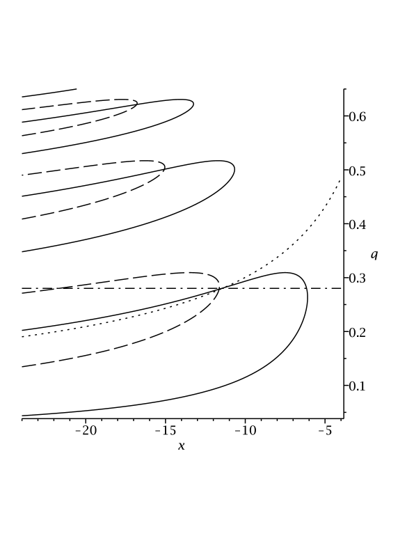
Figure 3. The real-zeros sets of $\theta(q,x)$ and $\theta(q,\sqrt{q}x)$.

Recall that the curves $\Gamma_{j}$ were defined in Theorem 3. One can define by analogy the curves $\Gamma_{j}^{*}$ for the set $\{(q,x)~{}|~{}\theta(q,\sqrt{q}x)=0\}$. On Fig. 3 one can see the intersection points of $\Gamma_{j}$ and $\Gamma_{j}^{*}$ for $j=1$, $2$ and $3$. Through the point $Z_{1}:=\Gamma_{1}\cap\Gamma_{1}^{*}$ passes a curve $x=-q^{-\gamma}$ with $\gamma\in(1,2)$. On Fig. 3 we represent this curve by dotted line and we draw by dash-dotted line the horizontal line $\mathcal{L}_{1}:\{q=q_{\bullet}\}$ passing through the point $Z_{1}$. The line $\mathcal{L}_{1}$ intersects each of the curves $\Gamma_{1}$ and $\Gamma_{1}^{*}$ at two points one of which is $Z_{1}$ (the left of the two points for $\Gamma_{1}$ and the right of the two for $\Gamma_{1}^{*}$). If one considers the graphs of the functions (in the variable $x$) $\theta(q_{\bullet},x)$ and $\theta(q_{\bullet},\sqrt{q_{\bullet}}x)$, then they will look like the two graphs drawn in solid line above left on Fig. 4; the point $Z_{1}$ will be the point $B$ on Fig. 4. Nevertheless one should keep in mind that Fig. 4 represents the graphs of two functions whose arguments are of the form $-qy^{2}$ and $-y^{2}/q$, i.e. increasing of $y>0$ corresponds to the decreasing of the (negative) values of these arguments.

The curve $x=-q^{-\gamma}$ and the line $\mathcal{L}_{1}$ were defined in relationship with $\Gamma_{1}$ and $\Gamma_{1}^{*}$, i.e. for $j=1$. One can consider their analogs defined for $j=2$, $3$, $\ldots$. Recall that the quantities $\kappa^{\triangle}$ and $q^{\triangle}$ were defined in Remarks 5. It is only for $j$ sufficiently large ($j\geq(\kappa^{\triangle}+1)/2$) that we have proved that the intersection of the curve $\Gamma_{j}$ with each curve $x=-q^{-a}$, $a\geq\kappa^{\triangle}$, is a point or is empty (see Proposition 3). For smaller values of $j$ we can claim only that this intersection (of two analytic curves) consists of not more than a finite number of points. This explains the final sentence of Theorem 10. ∎

Proof of Theorem 10.

To study the restriction of $\theta$ to the imaginary axis we set again

$$\theta^{\ddagger}(q,y):=\theta(q,iy)=f_{1}(q,y)+iqyf_{2}(q,y)~{}~{}~{}\,,~{}~{}~{}\,y\in\mathbb{R}~{},$$

where $f_{1}(q,y):=\theta(q^{4},-y^{2}/q)$ and $f_{2}(q,y):=\theta(q^{4},-qy^{2})$, see equalities (6.36) (in which we assume that $q\in(0,1)$). For $q$ close to $0$, the zeros of $\theta(q,x)$ are close to the numbers $-q^{-j}$, $j\in\mathbb{N}$. More precisely, for $q\in(0,0.108]$, there is a simple zero of $\theta$ of the form $-1/(q^{j}\Delta_{j})$ with $\Delta_{j}\in[0.2118,1.7882]$, and all these zeros are distinct, see Theorem 2.1 in [14]. Thus the zeros of $f_{1}(q,y)$ (resp. of $f_{2}(q,y)$) are close to the quantities $\pm q^{-2j+1/2}$ (resp. $\pm q^{-2j-1/2}$); hence the positive (resp. negative) zeros of $f_{1}$ interlace with the positive (resp. negative) zeros of $f_{2}$.

For $q>0$ small enough, all zeros of $\theta(q,.)$ are real negative; hence all zeros of $f_{1}$ are real. For such values of $q$, we denote the positive zeros of $f_{1}$ by $y^{\sharp}_{j}$, $y^{\sharp}_{j}<y^{\sharp}_{j+1}$ ($y^{\sharp}_{j}$ is close to $q^{-2j+1/2}$). As $q$ increases, these zeros depend continuously on $q$ and as we will see below, certain couples of them, for some values of $q$, coalesce and form complex conjugate pairs. Thus their indices are meaningful only till the value of $q$ corresponding to the moment of confluence.

As $f_{1}(q,y)=f_{2}(q,y/q)$, the positive zeros of $f_{2}$ equal $y^{\sharp}_{j}/q$. Consider the zeros $y^{\sharp}_{2j-1}$ and $y^{\sharp}_{2j}$ of $f_{1}$ and the zeros $y^{\sharp}_{2j-1}/q$ and $y^{\sharp}_{2j}/q$ of $f_{2}$. For values of $q$ close to $0$, they satisfy the following inequalities (we indicate in the second row the powers of $q$ to which they are approximatively equal for $q$ close to $0$):

(6.38) $$\begin{array}[]{cccccccc}y^{\sharp}_{2j-1}&<&y^{\sharp}_{2j-1}/q&<&y^{\sharp}_{2j}&<&y^{\sharp}_{2j}/q&.\\ \\ q^{-4j+5/2}&&q^{-4j+3/2}&&q^{-4j+1/2}&&q^{-4j-1/2}&\end{array}$$

As $q$ increases, for $q^{4}=\tilde{q}_{j}$ (i.e. for $q=(\tilde{q}_{j})^{1/4}$), the zeros $y^{\sharp}_{2j-1}$ and $y^{\sharp}_{2j}$ of $f_{1}$ (hence the zeros $y^{\sharp}_{2j-1}/q$ and $y^{\sharp}_{2j}/q$ of $f_{2}$ as well) coalesce and then give birth to a complex conjugate pair. This means that for values of $q$ just before the moment of confluence one has

(6.39) $$y^{\sharp}_{2j-1}<y^{\sharp}_{2j}<y^{\sharp}_{2j-1}/q<y^{\sharp}_{2j}/q~{}.$$

Therefore there exists $q^{\dagger}_{j}\in(0,(\tilde{q}_{j})^{1/4})$ for which one has $y^{\sharp}_{2j-1}<y^{\sharp}_{2j}=y^{\sharp}_{2j-1}/q<y^{\sharp}_{2j}/q$, i.e. the real and imaginary parts of $\theta$ have a common zero $y^{\sharp}_{2j}=y^{\sharp}_{2j-1}/q$. This is a simple zero both for $f_{1}$ and $f_{2}$ (hence $iy$ is a simple zero of $\theta(q^{\dagger}_{j},.)$). Indeed, $y^{\sharp}_{2j}$ can be either a simple or a double zero of $f_{1}$; if it is a double one, then $y^{\sharp}_{2j}$ must coalesce with $y^{\sharp}_{2j-1}$ (this follows from part (2) of Theorem 1 and part (1) of Remarks 1); this happens for $q^{4}=\tilde{q}_{j}$ which contradicts $q^{\dagger}_{j}<(\tilde{q}_{j})^{1/4}$.

We have just shown that for $j\in\mathbb{N}$ (i.e. for infinitely-many values of $q=q^{\dagger}_{j}\in(0,1)$) the function $\theta$ has a simple conjugate pair of zeros on the imaginary axis. In what follows we can assume that $j\geq(\kappa^{\triangle}+1)/2$, see Remarks 5 and the above preparation of the proof of Theorem 10. Thus the quantity $q^{\dagger}_{j}$ is unique. The real zeros $\xi_{j}$ of $\theta(q,x)$ for $q\in(0,1)$ satisfy the following string of inequalities:

$$-q^{-2j}<\xi_{2j}<\xi_{2j-1}<-q^{-2j+1}$$

(see equation (6) in [9]). This implies the inequalities

$$-q^{-8j}<\tau_{2j}<\tau_{2j-1}<-q^{-8j+4}~{},$$

satisfied by the zeros of $\theta(q^{4},x)$, and as $y^{\sharp}_{j}=(-q\tau_{j})^{1/2}$, the inequalities

(6.40) $$\begin{array}[]{lcl}q^{-4j+5/2}<y^{\sharp}_{2j-1}<y^{\sharp}_{2j}<q^{-4j+1/2}&&{\rm and}\\ \\ q^{-4j+3/2}<y^{\sharp}_{2j-1}/q<y^{\sharp}_{2j}/q<q^{-4j-1/2}&&\end{array}$$

hold true. Inequalities (6.40) (see also (6.38) and (6.39)) imply that

i) the zero $y^{\sharp}_{2j}$ of $f_{1}$ can be equal to $y^{\sharp}_{2j-1}/q$ and to no other zero of $f_{2}$ and

ii) the zero $y^{\sharp}_{2j-1}$ of $f_{1}$ can be equal to neither of the zeros of $f_{2}$.

On Fig. 4 (above left, in solid line) we show the graphs of the functions $f_{1}(q^{\dagger}_{j},.)$ and $f_{2}(q^{\dagger}_{j},.)$ (they are denoted by “Re” and “Im” respectively). The points $A$, $B$ and $C$ indicate the positions of the zeros $y^{\sharp}_{2j-1}$, $y^{\sharp}_{2j}=y^{\sharp}_{2j-1}/q$ and $y^{\sharp}_{2j}/q$ respectively. By dotted lines we show these graphs for $q\in(q^{\dagger}_{j},(\tilde{q}_{j})^{1/4})$. We remind that (see the proof of Theorem 1 in [9]) as $q$ increases, the local minima of $\theta(q,.)$ go up; when $q$ runs over an interval $((\tilde{q}_{j})^{-},(\tilde{q}_{j})^{+})$, the two rightmost real zeros coalesce for $q=\tilde{q}_{j}$ and the function $\theta(\tilde{q}_{j},.)$ has a local minimum at this double zero.

Figure 4. The complex conjugate pairs of $\theta$ on the imaginary axis.

Consider the function $\theta(q,iy+\varepsilon)$, i.e. the restriction of $\theta$ to a line in the $x$-plane parallel to the imaginary axis and belonging to the right half-plane. One checks directly that

$$\begin{array}[]{cclc}\theta(q,iy+\varepsilon)&=&\theta(q,iy)+\varepsilon(\partial\theta/\partial x)(q,iy)+o(\varepsilon)&{\rm where}\\ \\ (\partial\theta/\partial x)(q,iy)&=&K_{1}+iK_{2}&,\\ \\ K_{1}&:=&\sum_{\nu=0}^{\infty}(-1)^{\nu}(2\nu+1)q^{(\nu+1)(2\nu+1)}y^{2\nu}&\\ \\ &=&2(-q^{2}y^{2})(\partial\theta/\partial x)(q^{4},-qy^{2})+q\theta(q^{4},-qy^{2})&,\\ \\ K_{2}&:=&\sum_{\nu=1}^{\infty}(-1)^{\nu}2\nu q^{\nu(2\nu+1)}y^{2\nu-1}&\\ \\ &=&2(y/q)(\partial\theta/\partial x)(q^{4},-y^{2}/q)&.\end{array}$$

The second term of $K_{1}$ vanishes at $B$. The first term equals

$$qy(-2qy)(\partial\theta/\partial x)(q^{4},-qy^{2})=qy(\partial f_{2}/\partial y)~{}.$$

As Im $\theta$ is decreasing at $B$, one sees that $K_{1}<0$. In the same way,

$$K_{2}=-(-2y/q)(\partial\theta/\partial x)(q^{4},-y^{2}/q)=-\partial f_{1}/\partial y~{}.$$

Looking at the graph of Re $\theta$ at the point $B$ one sees that Re $\theta$ is increasing there and one concludes that $K_{2}<0$.

On the right-hand of Fig. 4, we represent in solid line the sets Re $\theta=0$ and Im $\theta=0$ (in the $x$-plane, close to the point $B$ of the imaginary axis). These are the segments $hh^{\prime}$ and $gg^{\prime}$ respectively. The true sets are in fact not straight lines, but arcs whose tangent lines at $B$ look like $hh^{\prime}$ and $gg^{\prime}$; as $q$ varies, these arcs and their tangent lines change continuously.

Thus for $q=q^{\dagger}_{j}$, both quantities $K_{1}$ and $K_{2}$ are negative in the sector $S$. The graphs of Re $\theta(q,iy+\varepsilon)$ and Im $\theta(q,iy+\varepsilon)$ (considered as functions in $y$, for fixed $q$ and $\varepsilon$) are represented by dashed lines to the left below on Fig. 4.

As $q$ increases on $[q^{\dagger}_{j},(q^{\dagger}_{j})^{+})$, the values of Re $\theta$ and Im $\theta$ along the arcs $hh^{\prime}$ and $gg^{\prime}$ become positive (this corresponds to the fact that close to the point $B$, the graphs of $f_{1}$ and $f_{2}$ are above the $y$-axis for $q=(q^{\dagger}_{j})^{+}$, see the dotted graphs above left on Fig. 4). Hence the sets Re $\theta=0$ and Im $\theta=0$ shift as shown by dotted line on the right of Fig. 4 (it would be more exact to say that the tangent lines to these sets at $B$ shift like this). That is, their intersection point is in the right half-plane and the complex conjugate pair crosses the imaginary axis from left to right.

∎

References

- [1] G. E. Andrews, B. C. Berndt, Ramanujan’s lost notebook. Part II. Springer, NY, 2009.
- [2] B. C. Berndt, B. Kim, Asymptotic expansions of certain partial theta functions. Proc. Amer. Math. Soc. 139:11 (2011), 3779–3788.
- [3] K. Bringmann, A. Folsom and A. Milas, Asymptotic behavior of partial and false theta functions arising from Jacobi forms and regularized characters. J. Math. Phys. 58 (2017), no. 1, 011702, 19 pp.
- [4] K. Bringmann, A. Folsom, R. C. Rhoades, Partial theta functions and mock modular forms as -hypergeometric series, Ramanujan J. 29:1-3 (2012), 295-310. http://arxiv.org/abs/1109.6560
- [5] T. Creutzig, A. Milas and S. Wood, On regularised quantum dimensions of the singlet vertex operator algebra and false theta functions. Int. Math. Res. Not. IMRN 2017, no. 5, 1390–1432.
- [6] G. H. Hardy, On the zeros of a class of integral functions, Messenger of Mathematics, 34 (1904), 97–101.
- [7] J. I. Hutchinson, On a remarkable class of entire functions, Trans. Amer. Math. Soc. 25 (1923), 325–332.
- [8] O.M. Katkova, T. Lobova and A.M. Vishnyakova, On power series having sections with only real zeros. Comput. Methods Funct. Theory 3:2 (2003), 425–441.
- [9] V. P. Kostov, On the zeros of a partial theta function, Bull. Sci. Math. 137, No. 8 (2013) 1018-1030.
- [10] V. P. Kostov, On the double zeros of a partial theta function, Bull. Sci. Math. 140, No. 4 (2016) 98-111.
- [11] V. P. Kostov, A property of a partial theta function, Comptes Rendus Acad. Sci. Bulgare 67, No. 10 (2014) 1319-1326.
- [12] V. P. Kostov, The closest to spectral number of the partial theta function, Comptes Rendus Acad. Sci. Bulgare 69, No. 9 (2016) 1105-1112.
- [13] V. P. Kostov, On the multiple zeros of a partial theta function, Funct. Anal. Appl. 50, No. 2 (2016) 153-156.
- [14] V. P. Kostov, On the spectrum of a partial theta function, Proc. Royal Soc. Edinb. A 144, No. 5 (2014), 925-933.
- [15] V. P. Kostov, On a partial theta function and its spectrum, Proc. Royal Soc. Edinb. A 146, No. 3 (2016) 609-623.
- [16] V. P. Kostov, Asymptotics of the spectrum of partial theta function, Revista Mat. Complut. 27, No. 2 (2014) 677-684, DOI: 10.1007/s13163-013-0133-3.
- [17] V. P. Kostov, A domain containing all zeros of the partial theta function, Publicationes Mathematicae Debrecen (to appear).
- [18] V. P. Kostov and B. Z. Shapiro, Hardy-Petrovitch-Hutchinson’s problem and partial theta function, Duke Math. J. 162, No. 5 (2013) 825-861.
- [19] I. V. Ostrovskii, On zero distribution of sections and tails of power series, Israel Math. Conf. Proceedings, 15 (2001), 297–310.
- [20] M. Petrovitch, Une classe remarquable de séries entières, Atti del IV Congresso Internationale dei Matematici, Rome (Ser. 1), 2 (1908), 36–43.
- [21] G. Pólya, G. Szegő, Problems and Theorems in Analysis, Vol. 1, Springer, Heidelberg 1976.
- [22] A. Sokal, The leading root of the partial theta function, Adv. Math. 229:5 (2012), 2603-2621. arXiv:1106.1003.
- [23] S. O. Warnaar, Partial theta functions. I. Beyond the lost notebook, Proc. London Math. Soc. (3) 87:2 (2003), 363–395.