Weak coherent pulses for single-photon quantum memories

Abstract

Attenuated laser pulses are often employed in place for single photons in order to test the efficiency of the elements of a quantum network. In this work we analyse theoretically the dynamics of storage of an attenuated light pulse (where the pulse intensity is at the single photon level) propagating along a transmission line and impinging on the mirror of a high finesse cavity. Storage is realised by the controlled transfer of the photonic excitations into a metastable state of an atom confined inside the cavity and occurs via a Raman transition with a suitably tailored laser pulse, which drives the atom and minimizes reflection at the cavity mirror. We determine the storage efficiency of the weak coherent pulse which is reached by protocols optimized for single-photon storage. We determine the figures of merit and we identify the conditions on an arbitrary pulse for which the storage dynamics approaches the one of a single photon. Our formalism can be extended to arbitrary types of input pulses and to quantum memories composed by spin ensembles, and serves as a basis for identifying the optimal protocols for storage and readout.

I Introduction

Single photons are important elements for secure communication using light Afzelius2015 ; Sangouard2012 . Integrating single photons in a quantum network Ritter2012 , on the other hand, requires stable and efficient single photon sources, reliable storage units such as single-photon quantum memories, quantum information processors, and ideally dissipationless transmission channels Briegel1998 ; Kurizki2015 . Since these devices usually optimally work in different frequency regimes, the realization of efficient quantum networks implies the ability of interfacing hybrid elements Kurizki2015 ; Uphoff2016 . Proof-of-principle experiments for quantum memories have therefore often made use of pulses generated by stable lasers at the required frequency Choi2008 ; Kimble2008 ; Usmani2010 ; Lan2009 ; Gisin2007 ; Koerber2018 . The laser pulses are typically attenuated to the regime where the probability that they contain a single photon is very small, while the probability that two or more photons are detected is practically negligible. Even though photo-detection after a beam splitter shows the granular properties of the light, yet the coherence properties of weak laser pulses are quite different from the ones of a single photon Mack2003 . In particular, they are well described by coherent states of the electromagnetic field, whose correlation functions can be reproduced by a classical coherent field Glauber1963 ; Glauber1963a ; Schleich2001 . In this perspective it is therefore legitimate to ask which specific information about the efficiency of a single-photon quantum network can one possibly extract by means of weak laser pulses.

Theoretically, similar questions have been analysed in Ref. Fleischhauer2000 ; Gorshkov2007 ; Gorshkov2007a ; Gorshkov2007b ; Dilley2012 ; Kalachev2007 ; Kalachev2008 ; Kalachev2010 . In Fleischhauer2000 ; Gorshkov2007 ; Gorshkov2007a ; Gorshkov2007b ; Dilley2012 , in particular, the authors consider a quantum memory composed by an atomic ensemble, where the number of atoms is much larger than the mean number of photons of the incident pulse. In this limit the equations describing the dynamics can be brought to the form of the equations describing the interaction of a single photon with the medium, and one can simply extract from the study of one case the efficiency of the other. This scenario changes dramatically if the memory is composed by a single atom Cirac1997 ; Reiserer2015 ; Duan2010 ; Kurz2014 . In this case the dynamics is quite different depending on whether the atom interacts with a single photon or with (the superposition of) several photonic excitations.

In this work we theoretically analyse the dynamics of the storage of a weak coherent pulse into the excitation of a single-atom confined within an optical resonator like in the setups of Specht2011 ; Khudaverdyan2008 ; Kimble1998 ; Keller2004 . The laser pulse propagates along a transmission line and impinges on the mirror of the resonator, as illustrated in Fig. 1(a). A control laser drives the atom in order to optimize the transfer of the propagating pulse into the atomic excitation $|r\rangle$, as shown in Fig. 1(b). We determine the efficiency of storage under the assumption that the control laser optimizes the storage of a single photon, which possesses the same time dependent amplitude as the weak coherent pulse. Our goal is to identify the regime and the conditions for which the dynamics of storage of the weak coherent pulse reproduces the one of a single photon. This study draws on the protocols based on adiabatic transfer identified in Refs. Fleischhauer2000 ; Gorshkov2007a ; Dilley2012 ; Giannelli2018 . The theoretical formalism for the interface between the weak coherent pulse propagating along the transmission line and the single atom inside the resonator is quite general and can be extended to describe the storage fidelity of an arbitrary quantum state of light into excitations of the memory.

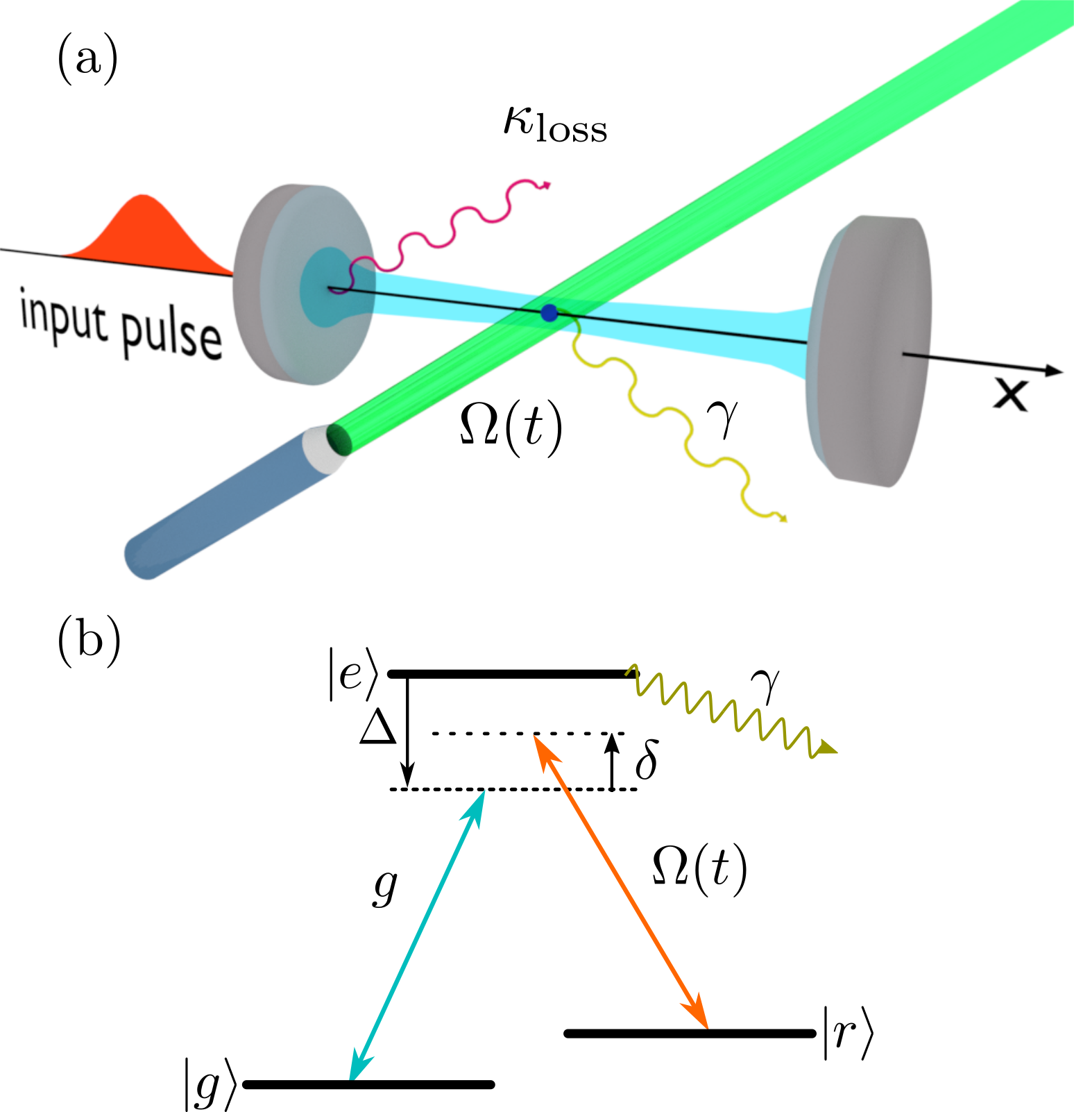
Figure 1: (Color online) An input pulse propagates along a transmission line and impinges onto a cavity mirror (a). The pulse is absorbed and the atom undergoes a Raman transition from the initial state $|g\rangle$ to the final state $|r\rangle$ via the common excited state $|e\rangle$. This dynamics occurs thanks to a laser with appropriately tailored Rabi frequency $\Omega(t)$, which drives the transition $|r\rangle\to|e\rangle$ in order to maximize the transfer to state $|r\rangle$ and simultaneously minimize reflection at the mirror. We analyse the dynamics of storage when the incident light is described by a weak coherent pulse and $\Omega(t)$ is designed to optimize storage of a single photon. Further parameters are defined in the text.

This manuscript is organized as follows. In Sec. II we introduce the theoretical model. In Sec. III we report our results: in Sec III.1 we analyse the storage fidelity of a weak coherent pulse. In Sec. III.2 we analyze the storage fidelity of an arbitrary incident pulse at the single photon level. We then compare them with the storage fidelity of a single photon. The conclusions are drawn in Sec. IV. The appendices provide details to the calculations in Secs. II and III.

II Basic model

Figure 1 reports the basic elements of the dynamics. A weak coherent pulse propagates along the transmission line and impinges on the mirror of a optical high-finesse cavity. Here it is transmitted into a cavity mode at frequency $\omega_{\mathrm{c}}$, which, in turn, interacts with a single atom confined within the resonator. The atom is driven by a laser, whose temporal shape is tailored in order to maximize the transfer of a single photonic excitation, with the same amplitude as the weak coherent pulse, into an atomic excitation $|r\rangle$.

In the following we provide the details of the theoretical model and we introduce the physical quantities which are important for the discussion of the rest of this paper.

II.1 Master equation

We describe the dynamics of storage by determining the density matrix $\hat{\rho}$ for the cavity mode, the atom, and the modes of the transmission line. Its evolution is governed by the master equation ($\hbar=1$)

$$\partial_{t}\hat{\rho}=-\mathrm{i}[\hat{H}_{\mathrm{tot}}(t),\hat{\rho}]+\mathcal{L}_{\mathrm{dis}}\hat{\rho}\,,$$ (1)

where Hamiltonian $\hat{H}_{\mathrm{tot}}(t)$ determines the coherent evolution and superoperator $\mathcal{L}_{\mathrm{dis}}$ the incoherent dynamics. Below we define them.

The Hamiltonian $\hat{H}$ describes the unitary dynamics of the system composed of the modes of the transmission line, the cavity mode, and the atom’s internal degrees of freedom. We decompose it into the sum of two terms

$$\hat{H}_{\mathrm{tot}}(t)=\hat{H}_{\mathrm{fields}}+\hat{H}_{\mathrm{I}}(t)\,.$$ (2)

The term $\hat{H}_{\mathrm{fields}}$ describes the coherent dynamics of the electromagnetic fields in absence of the atom. In the reference frame rotating at the cavity mode frequency $\omega_{\mathrm{c}}$ it reads

$$\hat{H}_{\mathrm{fields}}=\sum_{k}(\omega_{k}-\omega_{\mathrm{c}})\hat{b}_{k}^{\dagger}\hat{b}_{k}+\sum_{k}\lambda_{k}(\hat{a}^{\dagger}\hat{b}_{k}+\hat{b}_{k}^{\dagger}\hat{a}).$$ (3)

Here, $\omega_{k}$ are the frequencies of the electromagnetic field’s modes of the transmission line, operators $\hat{b}_{k}$ and $\hat{b}_{k}^{\dagger}$ annihilate and create, respectively, a photon at frequency $\omega_{k}$, with $[\hat{b}_{k},\hat{b}_{k^{\prime}}^{\dagger}]=\delta_{k,k^{\prime}}$. The modes $\hat{b}_{k}$ are formally obtained by quantizing the electromagnetic field in a resonator of length $L$, where $L$ is taken to be much larger than any other length in the system. They are standing wave modes with a node at the cavity mirror (here at $x=0$) and have the same polarization as the cavity mode (see Appendix A). The latter is described by a harmonic oscillator with annihilation and creation operators $a$ and $a^{\dagger}$, where $[\hat{a},\hat{a}^{\dagger}]=1$ and $[\hat{a},\hat{b}_{k}]=[\hat{a},\hat{b}_{k}^{\dagger}]=0$. In the rotating-wave approximation the interaction is of beam-splitter type and conserves the total number of excitations. The couplings $\lambda_{k}$ are related to the radiative damping rate $\kappa$ of the cavity mode by $\kappa=L|\lambda(\omega_{\mathrm{c}})|^{2}/c$, with $\lambda(\omega_{\mathrm{c}})$ the coupling strength at the cavity-mode resonance frequency Carmichael . Furthermore, using the Markov approximation, the couplings are taken to be $\lambda_{k}=\lambda(\omega_{\mathrm{c}})$.

The atom-photon interactions are treated in the dipole and rotating-wave approximations. The fields interact with two dipolar transitions sharing the common excited state $|e\rangle$, forming a $\Lambda$ level scheme, see Fig. 1(b). The transition $|g\rangle\to|e\rangle$ couples with the cavity mode with strength (vacuum Rabi frequency) $g$. Transition $|r\rangle\to|e\rangle$ is driven by a laser with the time-dependent Rabi frequency $\Omega(t)$. The corresponding Hamiltonian reads

$$\hat{H}_{\mathrm{I}}=\delta\left|r\middle>\!\middle<r\right|-\Delta\left|e\middle>\!\middle<e\right|+\left[g\left|e\middle>\!\middle<g\right|\hat{a}+\Omega(t)\left|e\middle>\!\middle<r\right|+\mathrm{H.c.}\right],$$ (4)

where $\Delta=\omega_{\mathrm{c}}-\omega_{e}$ is the detuning between the cavity frequency $\omega_{\mathrm{c}}$ and the frequency $\omega_{e}$ of the $|g\rangle-|e\rangle$ transition, while $\delta=\omega_{r}+\omega_{\mathrm{L}}-\omega_{\mathrm{c}}$ is the two-photon detuning which is evaluated using the central frequency $\omega_{\mathrm{L}}$ of the driving field $\Omega(t)$. Here, $\omega_{r}$ denotes the frequency difference (Bohr frequency) between the state $|r\rangle$ and the state $|g\rangle$. Unless otherwise stated, in the following we assume that the conditions of one and two-photon resonance $\Delta=\delta=0$ are fulfilled.

Superoperator $\mathcal{L}_{\mathrm{dis}}$ describes the incoherent dynamics due to spontaneous decay of the atomic excited state $|e\rangle$ at rate $\gamma$, and due to the finite transmittivity of the second cavity mirror as well as due to scattering and/or finite absorption of radiation at the mirror surfaces at rate ${\kappa_{\mathrm{loss}}}$. We model each of these phenomena by Born-Markov processes described by the superoperators $\mathcal{L}_{\gamma}$ and $\mathcal{L}_{{\kappa_{\mathrm{loss}}}}$, respectively, such that $\mathcal{L}_{\mathrm{dis}}=\mathcal{L}_{\gamma}+\mathcal{L}_{{\kappa_{\mathrm{loss}}}}$ and

$$\mathcal{L}_{\gamma}\hat{\rho}=\gamma(2\left|\xi_{e}\middle>\!\middle<e\right|\hat{\rho}\left|e\middle>\!\middle<\xi_{e}\right|-\left|e\middle>\!\middle<e\right|\hat{\rho}-\hat{\rho}\left|e\middle>\!\middle<e\right|)\,,$$ (5a)

$$\mathcal{L}_{\kappa_{\mathrm{loss}}}\hat{\rho}={\kappa_{\mathrm{loss}}}(2\hat{a}\hat{\rho}\hat{a}^{\dagger}-\hat{a}^{\dagger}\hat{a}\hat{\rho}-\hat{\rho}\hat{a}^{\dagger}\hat{a})\,.$$ (5b)

Here, $|\xi_{e}\rangle$ is an atomic state into which the excited state $|e\rangle$ decays, which is assumed to be different from $|g\rangle$ and $|r\rangle$.

II.2 Initial state

The total state of the system $|\psi_{t}\rangle$ at the initial time $t=t_{1}$ is given by a weak coherent pulse in the transmission line, the empty optical cavity, and the atom in state $|g\rangle$:

$$|\psi_{t_{1}}\rangle=|g\rangle\otimes|0\rangle_{c}\otimes|\psi^{\mathrm{coh}}\rangle,$$ (6)

where $|0\rangle_{c}$ is the Fock state of the resonator with zero photons.

Below we specify in detail the state of the field. The incident light pulse is characterized by the time-dependent operator $\hat{D}$, such that its state at the interface with the optical resonator reads

$$|\psi^{\mathrm{coh}}\rangle=\hat{D}(\{\alpha_{k}\})|\mathrm{vac}\rangle$$ (7)

and $|\mathrm{vac}\rangle$ is the vacuum state of the external electromagnetic field. Operator $\hat{D}(\{\alpha_{k}\})$ takes the form

$$\hat{D}(\{\alpha_{k}\})=\otimes_{k}\exp(\alpha_{k}\hat{b}_{k}^{\dagger}-\alpha_{k}^{*}\hat{b}_{k})\,,$$ (8)

where $\alpha_{k}$ is a complex scalar and the index $k$ runs over all modes of the electromagnetic field with the same polarization. It thus generates a multi-mode coherent state, whose mean photon number $n$ is

$$n=\langle\psi^{\mathrm{coh}}\vphantom{\psi^{\mathrm{coh}}}|\sum_{k}\hat{b}_{k}^{\dagger}\hat{b}_{k}|\psi^{\mathrm{coh}}\vphantom{\psi^{\mathrm{coh}}}\rangle=\sum_{k}|\alpha_{k}|^{2}\,.$$ (9)

In the following we assume that $n\ll 1$, which is fulfilled when $|\alpha_{k}|^{2}\ll 1$ for all $k$. We will denote this a weak coherent pulse. This state approximates a single-photon state since at first order in $n$ it can be approximated by the expression

$$|\psi^{\mathrm{coh}}\rangle\approx(1-n/2)|\mathrm{vac}\rangle+\sum_{k}\alpha_{k}\hat{b}_{k}^{\dagger}|\mathrm{vac}\rangle\,.$$ (10)

Coefficients $\alpha_{k}$ are related to the pulse envelope $\mathcal{E}_{\mathrm{in}}(t)$ at position $x=0$ (which is the position of the mirror interfacing the cavity with the transmission line) via the relation

$$\alpha_{k}=\sqrt{\frac{c}{2L}}\int_{-\infty}^{\infty}\mathrm{d}te^{\mathrm{i}(kc-\omega_{\mathrm{c}})t}\mathcal{E}_{\mathrm{in}}(t)$$ (11)

with $c$ the speed of light and $L$ the length of the transmission line. The squared norm of $\mathcal{E}_{\mathrm{in}}(t)$ equals the number of impinging photons in Eq. (9):

$$\int_{-\infty}^{\infty}|\mathcal{E}_{\mathrm{in}}(t)|^{2}\mathrm{d}t=n\,.$$ (12)

In this work we are interested in determining the storage efficiency of a weak coherent pulse by the atom. We compare in particular the storage efficiency with the one of a single photon, whose amplitude is given by the same amplitude $\mathcal{E}_{\mathrm{in}}(t)$, apart for a normalization factor giving that the integral in Eq. (12) is unity. For this specific study we choose

$$\mathcal{E}_{\mathrm{in}}(t)=\frac{\sqrt{n}}{\sqrt{T}}\operatorname{sech}{\left(\frac{2t}{T}\right)}\,,$$ (13)

where $T$ is the characteristic time determining the coherence time $T_{\mathrm{c}}=\pi T/4\sqrt{3}$ of the light pulse, defined as

$$T_{\mathrm{c}}=\sqrt{\langle t^{2}\rangle-\langle t\rangle^{2}}$$ (14)

with $\langle t^{x}\rangle\equiv\int_{t_{1}}^{t_{2}}t^{x}|\mathcal{E}_{\mathrm{in}}(t)|^{2}\mathrm{d}t$. The dynamics is analysed in the interval $t\in[t_{1},t_{2}]$, with $t_{1}<0<t_{2}$ and $|t_{1}|,t_{2}\gg T_{\mathrm{c}}$, such that (i) at the initial time there is no spatial overlap between the input light pulse and the cavity mirror and (ii) at $t=t_{2}$ the reflected component of the light pulse is sufficiently far away from the mirror so that it has no spatial overlap with the cavity mode. The choice of these parameters has been discussed in detail in Appendix A and in Ref. Giannelli2018 .

II.3 Target dynamics

The target of the dynamics is to absorb a single photon excitation and populate the atomic state $|r\rangle$. This dynamics is achieved by suitably tailoring the control field $\Omega(t)$. We will consider protocols using control fields $\Omega(t)$ that have been developed for a single-photon wave packet Fleischhauer2000 ; Gorshkov2007a ; Dilley2012 ; Giannelli2018 . The figures of merit we take are (i) the probability $\eta$ to find the excitation in the state $|r\rangle$ of the atom after a fixed interaction time and (ii) the fidelity of the transfer $\nu$, which we define as the ratio between the probability $\eta$ and the number of impinging photons. This ratio, as we show in the next section, approaches the fidelity of storage of a single photon $\eta^{\mathrm{sp}}$ when $n\to 0$.

We give the formal definition of these two quantities. The probability $\eta$ reads Gorshkov2007a

$$\eta=\operatorname{Tr}\left\{\hat{\rho}(t_{2})\left|r\middle>\!\middle<r\right|\otimes{\mathds{1}_{\mathrm{em}}}\right\}=\langle r\vphantom{r}|\operatorname{Tr}_{\mathrm{em}}\left\{\hat{\rho}(t_{2})\right\}|r\vphantom{r}\rangle$$ (15)

where $\mathds{1}_{\mathrm{em}}$ and $\operatorname{Tr}_{\mathrm{em}}$ denote respectively the identity and the trace over the electromagnetic fields (both the fields in the transmission line and in the optical cavity), and $\hat{\rho}(t)$ is the density operator of the system.

The fidelity of the transfer is defined as the ratio between $\eta$ and the number of impinging photons, namely

$$\nu=\frac{\eta}{\int_{t_{1}}^{t_{2}}|\mathcal{E}_{\mathrm{in}}(t)|^{2}\mathrm{d}t},$$ (16)

which is strictly valid for a coherent pulse. This definition of the fidelity quantitatively describes the probability that the incident pulse is stored by the atom. It agrees with the definition of Ref. Gorshkov2007a , where the authors denote this quantity by “efficiency”. Indeed, if the initial state is a single photon, the fidelity $\nu$ and the efficiency $\eta$ coincide.

Before we conclude, we remind the reader of the cooperativity $C$, which determines the maximum fidelity of single-photon storage Gorshkov2007a ; Giannelli2018 . The cooperativity $C$ characterizes the strength of the coupling between the cavity mode and the atomic transition, it reads Gorshkov2007a

$$C=\frac{g^{2}}{{\kappa_{\mathrm{tot}}}\gamma},$$ (17)

where ${\kappa_{\mathrm{tot}}}=\kappa+{\kappa_{\mathrm{loss}}}$ is the total cavity decay rate. For protocols based on adiabatic transfer of the single photon into the atomic excitation, the maximum fidelity of single-photon storage reads Gorshkov2007a ; Giannelli2018

$$\eta_{\mathrm{max}}^{\mathrm{sp}}=\frac{\kappa}{{\kappa_{\mathrm{tot}}}}\frac{C}{1+C}\,,$$ (18)

and it approaches $\kappa/{\kappa_{\mathrm{tot}}}$ for $C\to\infty$. Equation (18) is also the probability for emission of a photon into the transmission line when the atom is initially prepared in the excited state $|e\rangle$ and no control pulse is applied.

The parameters we use in our study are the ones of the setup of Ref. Koerber2018 , $(g,\kappa,\gamma,{\kappa_{\mathrm{loss}}})=(4.9,2.42,3.03,0.33)\times 2\pi\,\mathrm{MHz}$, corresponding to the cooperativity $C\approx 2.88$ and to the maximal storage fidelity $\eta_{\mathrm{max}}^{\mathrm{sp}}\approx 0.65$. Furthermore we choose $T_{\mathrm{c}}=0.5\,\mathrm{\mu s}$ such that the adiabatic condition is fulfilled: $\gamma T_{\mathrm{c}}C\approx 27\gg 1$ (see Ref. Giannelli2018 ).

III Storage

In this section we report the results of the storage of weak coherent pulses into a single atom excitation. We first determine efficiency and fidelity by numerically solving the master equation of Eq. (1). We compare the results with the corresponding storage fidelity of a single photon with temporal envelope $\mathcal{E}_{\mathrm{in}}(t)$, Eq. (13). We then determine analytically the efficiency $\eta$ and the fidelity $\nu$ for weak coherent pulses with mean photon number $n\ll 1$ and quantify the discrepancy between these quantities and the single-photon storage fidelity as a function of $n$. We further discuss how this method can be extended in order to determine the efficiency of storage of an arbitrary incident pulse.

III.1 Numerical results

We determine the dynamics of storage by numerically integrating a master equation in the reduced Hilbert space of cavity mode and atomic degrees of freedom, which we obtain from the master equation (1) after moving to the reference frame which displaces the multimode coherent state to the vacuum. The procedure extends to an input multi-mode coherent state an established procedure for describing the interaction of a quantum system with an oscillator in a coherent state, see for instance Cohen-Tannoudji1994 . We apply the unitary transformation $\hat{D}^{\prime}(t)=\hat{D}(\{\alpha_{k}(t)\})$, where operator $\hat{D}$ is given in Eq.(8) and the arguments are $\alpha_{k}\to\alpha_{k}(t)=\alpha_{k}e^{-\mathrm{i}(\omega_{k}-\omega_{\mathrm{c}})t}$. In this reference frame the initial state of the electromagnetic field is the vacuum, the full density matrix is given by $\hat{\rho}^{\prime}(t)=\hat{D}^{\prime}(t)^{\dagger}\rho(t)\hat{D}^{\prime}(t)$ and its coherent dynamics is governed by Hamiltonian

$$\hat{H}^{\prime}(t)={} \hat{H}_{\mathrm{tot}}(t)+\sqrt{2\kappa}\left(\mathcal{E}_{\mathrm{in}}(t)\hat{a}^{\dagger}+\mathcal{E}_{\mathrm{in}}^{*}(t)\hat{a}\right).$$ (19)

Here $\mathcal{E}_{\mathrm{in}}(t)$ carries the information about the initial state of the electromagnetic field and it is related to the amplitudes $\alpha_{k}$ by the following equation (consistently with Eq. (11))

$$\mathcal{E}_{\mathrm{in}}(t)=\sqrt{\frac{Lc}{2\pi^{2}}}\int_{-\infty}^{\infty}\alpha(k+k_{c})e^{-\mathrm{i}kct}\mathrm{d}k.$$ (20)

By using the Born-Markov approximation one can now trace out the degrees of freedom of the electromagnetic field outside the resonator. The Hilbert space is then reduced to the cavity mode and atom’s degrees of freedom, the density matrix which describes the state of this system is

$$\hat{\tau}(t)=\operatorname{Tr}_{\mathrm{ff}}{\hat{\rho}^{\prime}(t)}\,,$$ (21)

where $\operatorname{Tr}_{\mathrm{ff}}$ denotes the partial trace with respect to the degrees of freedom of the external electromagnetic field. Its dynamics is governed by the master equation

$$\partial_{t}\hat{\tau}=-\mathrm{i}[\hat{H}(t),\hat{\tau}]+\mathcal{L}_{\mathrm{\gamma}}\hat{\tau}+\mathcal{L}_{\mathrm{{\kappa_{\mathrm{tot}}}}}\hat{\tau}.$$ (22)

and superoperators $\mathcal{L}_{\gamma}$ and $\mathcal{L}_{\kappa_{\mathrm{tot}}}$ are defined in Eqs. (5), where now the cavity field is damped at rate ${\kappa_{\mathrm{tot}}}=\kappa+{\kappa_{\mathrm{loss}}}$ and $\kappa$ is the linewidth due to radiative decay of the cavity mode by the finite transmittivity of the mirror at $x=0$. The initial state is here described by the density operator $\hat{\tau}(t_{1})=\left|g,0_{c}\middle>\!\middle<g,0_{c}\right|$, and the storage efficiency is $\eta=\operatorname{Tr}\left\{\hat{\tau}(t_{2})\left|r\middle>\!\middle<r\right|\right\}$.

We integrate numerically the optical Bloch Equation for the matrix elements of Eq. (22) taking a truncated Hilbert space for the cavity field, with number states ranging from $m=0$ to $m=m_{\rm max}$. For the parameters we use in our simulation we find that the mean average number of intracavity photons is below 2. We check the convergence of our simulation for different values of $m=m_{\rm max}$ and fix $m_{\rm max}=14$. Figure 2 displays the storage efficiency $\eta$ and fidelity $\nu$ at time $t=t_{2}$ for different mean number of photons $n$ of the incident weak coherent pulse. When evaluating the dynamics we employed the control laser pulse $\Omega(t)$ which optimizes the storage of the incident pulse when this is a single photon with temporal envelope $\mathcal{E}_{\mathrm{in}}(t)$, Eq. (13). In detail, the amplitude of the laser pulse has been determined in Ref. Giannelli2018 and reads (for $\delta=\Delta=0$)

$$\Omega(t)=\sqrt{\frac{2\gamma(1+C)}{(e^{4t/T}+1)T}}.$$ (23)

We observe that the storage efficiency $\eta$ rapidly increases with $n$ and saturates to the asymptotic value $\eta_{\infty}\approx 0.79$ for $n\gtrsim 10$. This asymptotic value indicates that the field in the cavity is essentially classical, the dynamics is the one of STIRAP Vitanov2017 , and its efficiency does not reach unity being the control pulse optimal for single-photon storage but not for STIRAP. The fidelity $\nu$ decreases with $n$, while in the limit $n\to 0$ it approaches the single-photon storage fidelity. We note that the behavior for $n\gtrsim 1$ depends on the pulse shape (see Fig. 2).

In Ref. Koerber2018 the authors report the experimental results of measuring the fidelity $\nu$ as a function of $n$. In particular they report the ratio between the fidelity of storing a weak coherent pulse with $n\approx 0.02$ and the fidelity for $n\approx 1$ to be $\nu_{\mathrm{exp}}(n=0.02)/\nu_{\mathrm{exp}}(n=1)\approx 1.27$. We compare these results with our predictions for $n\ll 1$ where the fidelity is independent of the photon shape. Then, we extract the same ratio from Fig. 2 and obtain $\nu(n=0.02)/\nu(n=1)\approx 1.5$. Even if for $n=1$ the fidelity depends on the pulse shape, we have verified by comparing with different pulse shapes that the discrepancy is typically small.

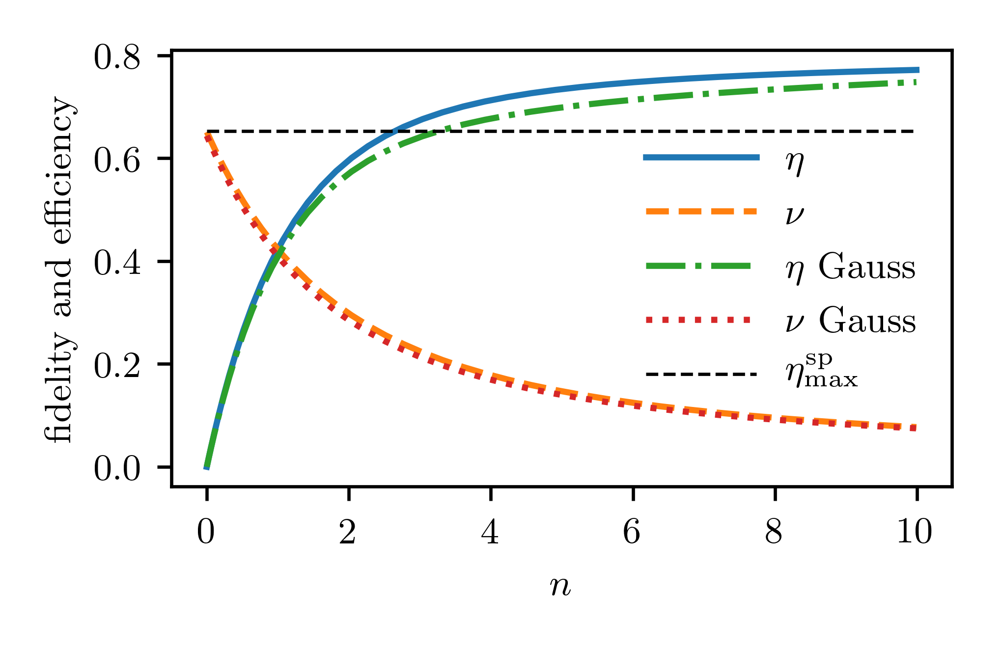
Figure 2: (Color online) Storage efficiency $\eta$, Eq. (15) and fidelity $\nu$, Eq. (16), at time $t=t_{2}$ as a function of the mean photon number $n$ of the incident weak coherent pulse with shape of Eq. (13) (solid and dashed). The figures of merit $\eta$ and $\nu$ have been evaluated by determining numerically the density matrix of the system $\tau(t_{2})$ from the initial state $\hat{\tau}(t_{1})=\left|g,0_{c}\middle>\!\middle<g,0_{c}\right|$ by integrating the master equation (22) in the truncated Hilbert space of the cavity field with a maximum of $14$ excitations. For comparison we also report the fidelity and efficiency of storage of a weak coherent pulse with Gaussian shape (labels “Gauss”); In this case the control pulse is optimized for the storage of a single photon with Gaussian shape. The dashed line indicates the maximal fidelity of storage of a single photon. The other parameters are given in Sec. II.3.

III.2 Extracting the single-photon storage fidelity from arbitrary incident pulses

The method we applied in Sec. III.1 is convenient but valid solely when the input pulse is a coherent state. We now show a more general approach for describing storage of a generic input pulse by an atomic medium (which can also be composed by a single atom) and which allows to obtain a useful description of the dynamics. This approach does not make use of approximations such as treating the atomic polarization as an oscillator Gorshkov2007a and allows one to determine the storage fidelity.

For this purpose we consider master equation (1), and recast it in the form Moelmer1988 ; Dum1992

$$\partial_{t}\hat{\rho}=-\mathrm{i}(\hat{H}_{\mathrm{eff}}(t)\hat{\rho}-\hat{\rho}\hat{H}_{\mathrm{eff}}^{\dagger}(t))+\mathcal{J}\hat{\rho},$$ (24)

where $\hat{H}_{\mathrm{eff}}(t)$ is a non-Hermitian operator, which reads

$$\hat{H}_{\mathrm{eff}}(t)=\hat{H}_{\mathrm{tot}}(t)-\mathrm{i}\gamma\left|e\middle>\!\middle<e\right|-\mathrm{i}{\kappa_{\mathrm{loss}}}\hat{a}^{\dagger}\hat{a}\,,$$ (25)

and is denoted in the literature as effective Hamiltonian. The last term on the right-hand side of Eq. (24) is denoted by jump term and is here given by

$$\mathcal{J}\hat{\rho}=2\left(\gamma\left|\xi_{e}\middle>\!\middle<e\right|\hat{\rho}\left|e\middle>\!\middle<\xi_{e}\right|+{\kappa_{\mathrm{loss}}}\hat{a}\hat{\rho}\hat{a}^{\dagger}\right).$$ (26)

This decomposition allows one to visualize the dynamics in terms of an ensemble of trajectories contributing to the dynamics, where each trajectory is characterized by a number of jumps at given instant of time within the interval where the evolution occurs Dum1992 ; Carmichael . Of all trajectories, we restrict to the one where no jump occurs since this is the only trajectory which contributes to the target dynamics. In fact, even though trajectories with spontaneous emission events may lead to dynamics where the atom is finally in state $|r\rangle$, yet such trajectories are incoherent and thus irreversible. We therefore discard them since they do not contribute to the fidelity of the process. The corresponding density matrix is $\rho_{0}(t)=S(t)\rho(t_{1})S(t)^{\dagger}/P_{0}$, where $S(t)=T:\exp\left(-i\int_{t_{1}}^{t}d\tau\hat{H}_{\mathrm{eff}}(\tau)/\hbar\right)$ and $T$ is the time ordering operator, while $P_{0}={\rm Tr}\{S(t)\rho(t_{1})S(t)^{\dagger}\}$ is the probability that the trajectory occurs. Since the initial state is a pure state, $\hat{\rho}(t_{1})=\left|\psi_{t_{1}}\middle>\!\middle<\psi_{t_{1}}\right|$, then $\hat{\rho}_{0}(t)=\left|\psi_{t}\middle>\!\middle<\psi_{t}\right|$ with $|\psi_{t}\rangle=S(t)|\psi_{t_{1}}\rangle/\sqrt{P_{0}}$. The efficiency of storage $\eta$, in particular, can be written as

$$\eta=P_{0}{\rm Tr}\{|r\rangle\langle r|\rho_{0}(t_{2})\}\,.$$ (27)

We note that this definition can be extended also to input pulses which are described by mixed states. In fact, consider the density matrix $\mu$ of the incident pulse: $\mu=\sum_{\alpha}p_{\alpha}\left|\psi^{\alpha}\middle>\!\middle<\psi^{\alpha}\right|$, with $\sum_{\alpha}p_{\alpha}=1$ and each $|\psi^{\alpha}\rangle$ a quantum state of the electromagnetic field. The efficiency of storage of the mixed state $\mu$ is then

$$\eta^{\mathrm{mix}}=\sum_{\alpha}p_{\alpha}\eta^{\alpha}\,.$$ (28)

Here, $\eta^{\alpha}$ is the efficiency of storage of the pure state $|\psi^{\alpha}\rangle$ which can be computed using Eq. (27).

In order to determine $\eta$, we first decompose the incident pulse at $t=t_{1}$ into photonic excitations, namely:

$$|\psi^{\rm coh}\rangle=\sum_{m=0}^{\infty}C_{m}|\psi^{(m)}\rangle,$$ (29)

where $\sum_{m}|C_{m}|^{2}=1$, and the state $|\psi^{(m)}\rangle$ contains exactly $m$ photons, $\langle\psi^{(\ell)}|\psi^{(m)}\rangle=\delta_{\ell,m}$. The dynamics transfers the excitations but preserves their total number, since $\hat{H}_{\mathrm{eff}}$ commutes with $\sum_{k}b_{k}^{\dagger}b_{k}+a^{\dagger}a+\left|e\middle>\!\middle<e\right|+\left|r\middle>\!\middle<r\right|$. Therefore it does not couple states $|\psi^{(m)}\rangle$ with different number of photons. By this decomposition we can numerically determine the fidelity $\eta$ for a finite number of initial excitations, as we show in Appendix B. The efficiency $\eta$, in particular, can be cast in the form

$$\eta=\sum_{m=0}^{\infty}|C_{m}|^{2}\eta^{(m)}\,,$$ (30)

where $\eta^{(m)}=\langle\psi^{(m)}|S(t)^{\dagger}|r\rangle\langle r|S(t)|\psi^{(m)}\rangle$ is the efficiency that one photon from a $m$-photon state is transferred into the atomic excitation $|r\rangle$. Here, $\eta^{(1)}$ is the storage fidelity of a single photon $\eta^{\mathrm{sp}}$. For a weak coherent pulse $C_{m}=\sqrt{e^{-n}n^{m}/m!}$, and for $n\ll 1$ we obtain the expression

$$\eta=n\eta^{(1)}+n^{2}\left(\eta^{(2)}/2-\eta^{(1)}\right)+O(n^{3})\,.$$ (31)

such that the fidelity takes the form

$$\nu=\frac{\eta}{n}=\eta^{(1)}+n\left(\eta^{(2)}/2-\eta^{(1)}\right)+O(n^{2})\,.$$ (32)

If the control pulse $\Omega(t)$ is chosen to be the one which maximize the storage fidelity of a single photon, then $\eta^{(1)}=\eta^{\mathrm{sp}}_{\mathrm{max}}$, Eq. (18). This can be clearly seen in Fig. 2.

We now discuss this dynamics if, instead of a single atom, the quantum memory is composed by $M$ atoms within the resonator. In the following we assume that the atoms are identical and that the vacuum Rabi coupling and the control laser pulse intensity and phase do not depend on the atomic positions within the cavity. Let us first consider that the input pulse is a single photon. In this case the dynamics can be mapped to the one described by Eq. (1), where in the Hamiltonian (4) the states of the $\Lambda$ transition are replaced by the collective atomic states $|g\rangle\to|g^{\prime}\rangle=|g_{1},\ldots,g_{M}\rangle$, $|e\rangle\to|e^{\prime}\rangle=\sum_{i=1}^{M}|g_{1},\dots,e_{i},\dots,g_{M}\rangle/\sqrt{M}$, and $|r\rangle\to|r^{\prime}\rangle=\sum_{i=1}^{M}|g_{1},\dots,r_{i},\dots,g_{M}\rangle/\sqrt{M}$, where the latter is the target state. For a single incident photon, in fact, these are the only internal states involved in the dynamics. The coupling between the cavity mode and the $|g^{\prime}\rangle-|e^{\prime}\rangle$ transition is now $g\sqrt{M}$, leading to a higher cooperativity $C$ and thus to a larger value of $\eta_{\mathrm{max}}^{\mathrm{sp}}$. In this case the control pulse leading to optimal storage is the same as for a single atom, which couples to the cavity with vacuum Rabi frequency $\tilde{g}=g\sqrt{M}$ (see for example Eq. (23) and Ref. Giannelli2018 ).

If the incident pulse is not a single photon, further collective excitations of the atoms have to be accounted for and the dynamics cannot be reduced to the coupling of a $\Lambda$ structure with the cavity field, as is detailed in Appendix B for the case of a weak coherent pulse. Nevertheless, if the number of atoms is much larger than the mean number of excitations in the incident pulse $M\gg n$, the dynamical equations can be reduced to the ones describing storage of the single photon Fleischhauer2000 ; Gorshkov2007a ; Dilley2012 . In this limiting case, the optimal control pulses for storage of a single photon can also be applied to storage of the input pulse by the atomic ensemble, as long as the input pulse has the same envelope as the single photon. We refer the interested reader to Ref. Gorshkov2007a for details.

In general, the formalism of the effective Hamiltonian can be applied to determine the control field for storage of an arbitrary input pulse by an atomic ensemble, without having to impose the condition $M\gg n$. For an arbitrary input pulse, $|\psi\rangle=\sum_{m=0}^{\infty}C_{m}|\psi^{(m)}\rangle$ with $\sum_{m}|C_{m}|^{2}=1$, the target state is $\sum_{m=0}^{\infty}C_{m}|r_{m}\rangle$, where $|r_{m}\rangle$ is the Dicke state of the atomic ensemble where $m$ atoms are in $|r\rangle$ and which is coherently coupled to the Dicke state $|g^{\prime}\rangle$ by the dynamics. The control pulse $\Omega(t)$ shall then optimize the dynamics by maximizing the fidelity

$$\eta^{\prime}=\sum_{m}|C_{m}|^{2}\eta_{m}^{(m)}\,,$$ (33)

where $\eta_{m}^{(m)}=\langle\psi^{(m)}|S(t)^{\dagger}|r_{m}\rangle\langle r_{m}|S(t)|\psi^{(m)}\rangle$ and $S(t)$ is calculated for the effective Hamiltonian of the atomic ensemble. The control field $\Omega(t)$ can be found by means of an analogous strategy as for ensemble optimal control theory (OCT), finding the control pulse that optimizes the dynamics in each subspace of $m$ excitations so to maximize $\eta^{\prime}$ Rojan2014 ; Goerz2014 ; Kobzar2004 ; Kobzar2008 ; Koch2016 .

IV Conclusions

We have analysed the storage of a weak coherent pulse into the excitation of a single atom inside a resonator, which acts as a quantum memory. Our specific objective was to characterize the process in order to show under which conditions an attenuated incident pulse can be considered as a single photon for storage purposes. Thus we have identified the conditions and the figures of merit which allow one to extract the single-photon storage fidelity by measuring the probability that the atom has been excited at the end of the process.

We remark that the retrieved information by a single atom will always be a single photon Chaneliere2005 . Nevertheless, the formalism we developed in this work permits one to extend this dynamics to other kind of incident pulses and to quantum memories composed by spin ensembles. For this general case it sets the basis for identifying the optimal control pulses for storage and retrieval of an arbitrary quantum light pulse.

Appendix A Description of the electromagnetic field in the transmission line

The transmission line is here modelled by a cavity of length $L$, with a perfect mirror at $x=-L$ and the second mirror at $x=0$, which corresponds to the optical cavity mirror with finite transmittivity. The modes of the transmission line are standing waves with wave vector along the $x$ axis. For numerical purposes we take a finite number $N$ of modes about the cavity wave number $k_{\mathrm{c}}=\frac{\omega_{\mathrm{c}}}{c}$. Their wave numbers are

$$k_{n}=k_{\mathrm{c}}+\frac{n\pi}{L}\,,$$ (34)

and $n=-(N-1)/2,\dots,(N-1)/2$, the corresponding frequencies are $\omega_{n}=ck_{n}$. We calibrate $N$ and $L$ so that our simulations are not significantly affected by the finite size of the transmission line and by the cutoff in the mode number $N$. For the propagation of the incident pulse and its appropriate description at the mirror interface, this requires that the difference between neighbouring frequencies is much smaller than the characteristic frequencies of the problem. We further choose $N$ in order to cover a frequency range which includes all the relevant frequencies of this system. With the choice $|t_{1}|=t_{2}=6T_{\mathrm{c}}$, $L=12cT_{\mathrm{c}}$ and $N=311$, the norm of the envelope results

$$\int_{t_{1}}^{t_{2}}|\mathcal{E}_{\mathrm{in}}(t)|^{2}\mathrm{d}t=n(1-\varepsilon)$$ (35)

with $\varepsilon<10^{-5}$. Further parameters and discussions are found in Ref. Giannelli2018 .

Appendix B Storage Efficiency for $n\ll 1$.

In this appendix we provide the details for calculating the dynamics and the fidelity for an incident pulse which is a superposition of different photon number states. We apply the procedure to multimode coherent states, nevertheless it can be generalised in a straighforward manner to a generic initial input pulse.

B.0.1 Decomposition of a coherent state

The coherent state in Eq. (7) can be decomposed in a linear combination of states each with a fixed number of excitations (see Eq. (29) with $C_{m}=\sqrt{e^{-n}n^{m}/m!}$): The mean number of photons in the mode $k$ is $|\alpha_{k}|^{2}$ and the mean photon number in the coherent state is $n=\sum_{k=1}^{N}|\alpha_{k}|^{2}$, see Eq. (9). State $|\psi^{(m)}\rangle$ contains exactly $m$ excitations of the quantum electromagnetic field and reads

$$|\psi^{(0)}\rangle{}=|\text{vac}\rangle,$$ (36a)

$$|\psi^{(1)}\rangle{}=\sum_{k=1}^{N}\mathcal{E}_{k}\hat{b}_{k}^{\dagger}|\text{vac}\rangle,$$ (36b)

$$|\psi^{(2)}\rangle{}=\sum_{k=1}^{N}\sum_{k^{\prime}=1}^{N}\mathcal{E}_{k,k^{\prime}}\hat{b}_{k}^{\dagger}\hat{b}_{k^{\prime}}^{\dagger}|\text{vac}\rangle,$$ (36c)

$$\vdots$$

$$|\psi^{(m)}\rangle{}=\sum_{\{k\}_{m}}\mathcal{E}_{\{k\}_{m}}\overbrace{\hat{b}_{k}^{\dagger}\hat{b}_{k^{\prime}}^{\dagger}\dots\hat{b}_{k^{\prime}{{}^{\prime\cdots}}^{\prime\prime}}^{\dagger}}^{m}|\text{vac}\rangle.$$ (36d)

Coefficients $\mathcal{E}_{\{k\}_{m}}$ read

$$\mathcal{E}_{k}=\frac{\alpha_{k}}{\sqrt{n}},$$ (37a)

$$\mathcal{E}_{k,k^{\prime}}=\mathcal{E}_{k^{\prime},k}=\frac{\mathcal{E}_{k}\mathcal{E}_{k^{\prime}}}{\sqrt{2}},$$ (37b)

$$\vdots$$ (37c)

$$\mathcal{E}_{\{k\}_{m}}=\mathcal{E}_{\underbrace{{}_{k,k^{\prime}\dots k^{\prime}{{}^{\prime\cdots}}^{\prime\prime}}}_{m}}=\frac{\prod_{i\in\{k\}_{m}}\mathcal{E}_{i}}{\sqrt{m!}},$$ (37d)

and it is easy to check that the states $|\psi^{(m)}\rangle$ are orthonormal $\langle\psi^{(m)}|\psi^{(n)}\rangle=\delta_{mn}$ and complete.

The storage fidelity when the initial state is the coherent state introduced in Eq. (29) is given by (see Eq. (30))

$$\eta=e^{-n}\sum_{m=1}^{\infty}\frac{n^{m}}{m!}\eta^{(m)}.$$ (38)

B.0.2 Equations of motion

We here explicitly derive the equations of motion in the subspaces with $m\leq 2$ excitations.

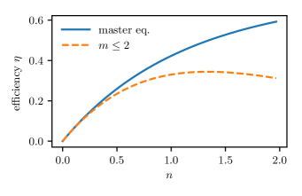
Figure 3: (Color online) Efficiency $\eta$ of the storage process of a weak coherent pulse. Solution with the master equation formalism of Sec. III.1 (solid line) and approximated solution with truncation to two excitations $m\leq 2$ as described in the current section (dashed).

Zero excitations - Vacuum: The subspace of zero excitations $m=0$ contains only the state $|g,0,\text{vac}\rangle$, meaning that the atom is in the ground state $|g\rangle$, the cavity is empty and the electromagnetic field is in the vacuum state. Thus the time evolution in this subspace is $|\phi^{(0)}_{t}\rangle=|\phi^{(0)}_{t_{1}}\rangle$.

One excitation - Single photon: A basis for the subspace with one excitation $m=1$ is

$$\mathcal{B}_{1}=\{ |g,1,\text{vac}\rangle,|e,0,\text{vac}\rangle,|r,0,\text{vac}\rangle,$$

$$|g,0,1_{k}\rangle:k\in\{1,\dots,N\}\}$$

and a general state can be written as

$$|\phi^{(1)}_{t}\rangle={} c_{1}(t)|g,1,\text{vac}\rangle+e_{1}(t)|e,0,\text{vac}\rangle+{}$$ (39)

$${}+r_{1}(t)|r,0,\text{vac}\rangle+\sum_{k}\mathcal{E}_{k}(t)|g,0,1_{k}\rangle.$$

The equations of motion in this subspace are ($\lambda_{k}=\lambda$)

$$\begin{gathered}\dot{c}_{1}(t)=-\mathrm{i}ge_{1}(t)-\mathrm{i}\lambda\sum_{k}\mathcal{E}_{k}(t)-{\kappa_{\mathrm{loss}}}c_{1}(t),\\ \dot{e}_{1}(t)=(\mathrm{i}\Delta-\gamma)e_{1}(t)-\mathrm{i}gc_{1}(t)-\mathrm{i}\Omega(t)r_{1}(t),\\ \dot{r}_{1}(t)=-\mathrm{i}\Omega^{*}(t)e_{1}(t),\\ \dot{\mathcal{E}}_{k}(t)=-\mathrm{i}\Delta_{k}\mathcal{E}_{k}(t)-\mathrm{i}\lambda c_{1}(t),\end{gathered}$$ (40)

and they constitute a system of $(N+3)$ coupled differential equations with time dependent coefficients. Using the input output formalism Walls1994 one obtains

$$\begin{gathered}\dot{c}_{1}(t)=-\mathrm{i}ge_{1}(t)-\mathrm{i}\sqrt{2\kappa}\mathcal{E}_{\mathrm{in}}(t)-(\kappa+{\kappa_{\mathrm{loss}}})c_{1}(t),\\ \dot{e}_{1}(t)=(\mathrm{i}\Delta-\gamma)e_{1}(t)-\mathrm{i}gc_{1}(t)-\mathrm{i}\Omega(t)r_{1}(t),\\ \dot{r}_{1}(t)=-\mathrm{i}\Omega^{*}(t)e_{1}(t),\end{gathered}$$ (41)

where $\kappa=L\lambda^{2}/c$ is the decay rate of the cavity field and $\mathcal{E}_{\mathrm{in}}(t)$ is defined in Eq. (20). Equations (40) or Eqs. (41) can be easily solved numerically. These equations correspond to the storage of a single photon into a single atom Giannelli2018 and are equivalent to the approximated equations obtained in Ref. Gorshkov2007a describing the storage of a light pulse in an atomic ensemble composed by a large number $N\gg 1$ of atoms.

Two excitations - Two photons states: A basis for the subspace with two excitations $m=2$ is

$$\mathcal{B}_{2}=\{ |g,2,\text{vac}\rangle,|g,1,1_{k}\rangle,|g,0,1_{k}1_{k^{\prime}}\rangle,|e,1,\text{vac}\rangle,$$

$$|e,0,1_{k}\rangle,|r,1,\text{vac}\rangle,|r,0,1_{k}\rangle:k,k^{\prime}\in\{1,\dots,N\}\}$$

thus a general state in this subspace can be written as

$$|\phi^{(2)}_{t}\rangle={} c_{2}(t)|g,2,\text{vac}\rangle+\sum_{k}\mathcal{E}_{k}^{c}(t)|g,1,1_{k}\rangle+{}$$ (42)

$${}+\sum_{k}\sum_{k^{\prime}\geq k}\mathcal{E}_{k,k^{\prime}}(t)|g,0,1_{k}1_{k^{\prime}}\rangle+{}$$

$${}+e_{2}(t)|e,1,\text{vac}\rangle+\sum_{k}\mathcal{E}_{k}^{e}(t)|e,0,1_{k}\rangle+{}$$

$${}+r_{2}(t)|r,1,\text{vac}\rangle+\sum_{k}\mathcal{E}_{k}^{r}(t)|r,0,1_{k}\rangle.$$

The state in Eq. (42) can be used to describe the interaction of the atom-cavity system with a two-photon state; in fact the term $\sum_{k,k^{\prime}}\mathcal{E}_{k,k^{\prime}}(t)|g,0,1_{k}1_{k^{\prime}}\rangle$ describes a two-photon state of the electromagnetic field. Notice that we use the definition $|\cdot,\cdot,1_{k}1_{k^{\prime}}\rangle=b_{k}^{\dagger}b_{k^{\prime}}^{\dagger}|\cdot,\cdot,\text{vac}\rangle$ which implies $|\cdot,\cdot,1_{k}1_{k}\rangle=\sqrt{2}|\cdot,\cdot,2_{k}\rangle$. The equations of motion in this subspace are

$$\begin{aligned} \dot{c_{2}}(t)=&-\mathrm{i}\sqrt{2}ge_{2}(t)-\mathrm{i}\sqrt{2}\lambda\sum_{k}\mathcal{E}_{k}^{c}(t)+{}\\ &{}-2{\kappa_{\mathrm{loss}}}c_{2}(t)\end{aligned}$$ (43)

$$\begin{aligned} \dot{e_{2}}(t)={}&\left(\mathrm{i}\Delta-\gamma-{\kappa_{\mathrm{loss}}}\right)e_{2}(t)-\mathrm{i}\sqrt{2}gc_{2}(t)+{}\\ &{}-\mathrm{i}\Omega(t)r_{2}(t)-\mathrm{i}\lambda\sum_{k}\mathcal{E}_{k}^{e}(t)\end{aligned}$$

$$\dot{r_{2}}(t)=-\mathrm{i}\Omega^{*}(t)e_{2}(t)-\mathrm{i}\lambda\sum_{k}\mathcal{E}_{k}^{r}(t)-{\kappa_{\mathrm{loss}}}r_{2}(t)$$

$$\begin{aligned} \dot{\mathcal{E}}_{k}^{c}(t)=&-\left(\mathrm{i}\Delta_{k}+{\kappa_{\mathrm{loss}}}\right)\mathcal{E}_{k}^{c}(t)-\mathrm{i}g\mathcal{E}_{k}^{e}(t)+{}\\ &{}-\mathrm{i}\lambda\sum_{k^{\prime}}A_{k,k^{\prime}}(t)-\mathrm{i}\sqrt{2}\lambda c_{2}(t)\end{aligned}$$

$$\begin{aligned} \dot{\mathcal{E}}_{k}^{e}(t)={}&\mathrm{i}\left(\Delta-\Delta_{k}\right)\mathcal{E}_{k}^{e}(t)-\mathrm{i}g\mathcal{E}_{k}^{c}(t)+{}\\ &{}-\mathrm{i}\Omega(t)\mathcal{E}_{k}^{r}(t)-\mathrm{i}\lambda e_{2}(t)\end{aligned}$$

$$\dot{\mathcal{E}}_{k}^{r}(t)=-\mathrm{i}\Delta_{k}\mathcal{E}_{k}^{r}(t)-\mathrm{i}\Omega^{*}(t)\mathcal{E}_{k}^{e}(t)-\mathrm{i}\lambda r_{2}(t)$$

$$\begin{aligned} \dot{A}_{k,k^{\prime}}(t)={}&-\mathrm{i}\left(\Delta_{k}+\Delta_{k^{\prime}}\right)A_{k,k^{\prime}}+{}\\ &{}-\mathrm{i}\lambda\left(\mathcal{E}_{k}^{c}(t)+\mathcal{E}_{k^{\prime}}^{c}(t)\right),\end{aligned}$$

where we have defined $A_{k,k^{\prime}}(t)=\mathcal{E}_{k,k^{\prime}}(t)+\mathcal{E}_{k^{\prime},k}(t)$. Eqs. (43) are a system of $(N^{2}+3N+3)$ coupled differential equations with time dependent coefficients; this system can be solved numerically.

Calculation of the efficiency The efficiency $\eta$ can be calculated with the formalism introduced in this section in two ways: (i) solve Eqs. (40) and Eqs. (43) with initial conditions given by the expansion (29) and the coefficients given by Eqs. (37a) and (37b), then the efficiency is

$$\eta=|r_{1}(t_{2})|^{2}+|r_{2}(t_{2})|^{2}+\sum_{k}|\mathcal{E}_{k}^{r}(t_{2})|^{2};$$ (44)

or (ii) solve Eqs. (40) and Eqs. (43) with initial conditions (37a) and (37b) separately to obtain the efficiencies $\eta^{(1)}$ and $\eta^{(2)}$ of single and double photon storage; then the efficiency as function of $n$ is given by Eq. (31).

Fig. 3 reports the efficiency $\eta$ as a function of $n$, the solid line represent the result of the numerical integration of the master equation described in Sec. III.1. The dashed line is the solution with the decomposition until $m=2$ described in this section. It is evident that for $n\ll 1$ the two results coincide.

References

- (1) M. Afzelius, N. Gisin, and H. de Riedmatten, Physics Today 68, 42 (2015).
- (2) N. Sangouard and H. Zbinden, Jour. of Mod. Opt., 59:17, 1458-1464 (2012).
- (3) S. Ritter, C. Nölleke, C. Hahn, A. Reiserer, A. Neuzner, M. Uphoff, M. Mücke, E. Figueroa, J. Bochmann, and G. Rempe, Nature 484, 195-200 (2012).
- (4) H.-J. Briegel, W. Dür, J. I. Cirac, and P. Zoller, Phys. Rev. Lett. 81, 5932 (1998)
- (5) G. Kurizki, P. Bertet, Y. Kubo, K. Mølmer, D. Petrosyan, P. Rabl, J. Schmiedmayer, PNAS 112 13 3866-3873 (2015).
- (6) M. Uphoff, M. Brekenfeld, G. Rempe, and S. Ritter, Appl. Phys. B 122, 46 (2016).
- (7) K. S. Choi, H. Deng, J. Laurat, and H. J. Kimble, Nature 452, 67–71 (2008).
- (8) H. J. Kimble, Nature 453, 1023 (2008).
- (9) I. Usmani, M. Afzelius, H. de Riedmatten, and N. Gisin, Nat. Comm. 1, 12 (2010).
- (10) S.-Y. Lan, A. G. Radnaev, O. A. Collins, D. N. Matsukevich, T. A. B. Kennedy, and A. Kuzmich, Opt. Expr. 17 16, 13639-13645 (2009).
- (11) N. Gisin, and R. Thew, Nat. Phot. 1, 165–171 (2007).
- (12) M. Körber, O. Morin, S. Langenfeld, A. Neuzner, S. Ritter, and G. Rempe, Nat. Phot. 12, 18-21 (2018).
- (13) H. Mack and P. W. Schleich, OPN Trends 3, 29-35 (2003).
- (14) R. J. Glauber, Phys. Rev. 130, 2529 (1963).
- (15) R. J. Glauber, Phys. Rev. 131, 2766 (1963).
- (16) W. P. Schleich, Quantum optics in phase space, WILEY-VCH (Berlin, 2001).
- (17) M. Fleischhauer, S.F. Yelin, and M.D. Lukin, Opt. Commun. 179, 395 (2000).
- (18) A. V. Gorshkov, A. André, M Fleischhauer, A. S. S Sørensen, and M. D. Lukin Phys. Rev. Lett. 98, 123601(2007).
- (19) A. V. Gorshkov, A. André, M. D. Lukin, and A. S. Sørensen, Phys. Rev. A 76, 033804 (2007).
- (20) A. V. Gorshkov, A. André, M. D. Lukin, and A. S. Sørensen, Phys. Rev. A 76, 033805 (2007).
- (21) J. Dilley, P. Nisbet-Jones, B. W. Shore, and A. Kuhn, Phys. Rev. A 85, 023834 (2012).
- (22) A. Kalachev, Phys. Rev. A 76, 043812 (2007).
- (23) A. Kalachev, Phys. Rev. A 78, 043812 (2008).
- (24) A. Kalachev, Opt. Spectrosc. 109, 32 (2010).
- (25) J. I. Cirac, P. Zoller, H. J. Kimble, and H. Mabuchi, Phys. Rev. Lett. 78, 3221 (1997).
- (26) A. Reiserer and G. Rempe, Rev. Mod. Phys. 87, 1379 (2015).
- (27) L.-M. Duan and C. Monroe, Rev. Mod. Phys. 82, 1209 (2010).
- (28) C. Kurz, M. Schug, P. Eich, J. Huwer, P. Müller, and J. Eschner, Nat. Commun. 5, 5527 (2014).
- (29) H. P. Specht, C. Nölleke, A. Reiserer, M. Uphoff, E. Figueroa, S. Ritter, and G. Rempe, Nature 473, 190–193 (2011).
- (30) M. Khudaverdyan, W. Alt, I. Dotsenko, T. Kampschulte, K. Lenhard, A. Rauschenbeutel, S. Reick, K. Schörner, A. Widera, and D. Meschede, New J. Phys. 10, (2008)
- (31) H. J. Kimble, Phys. Scr. 127, (1998).
- (32) M. Keller, B. Lange, K. Hayasaka, W. Lange, and H. Walther, New J. Phys. 6, (2004).
- (33) L. Giannelli, T. Schmit, T. Calarco, C. P. Koch, S. Ritter, and G. Morigi, preprint arXiv:1804.10558, (2018).
- (34) C. Cohen-Tannoudji, J. Dupont-Roc, and G. Grynberg, Atom-Photon Interactions, (Wiley-VCH, 2004).
- (35) N. V. Vitanov, A. A. Rangelov, B. W. Shore, and K. Bergmann, Rev. Mod. Phys. 89, 015006 (2017).
- (36) R. Dum, P. Zoller, and H. Ritsch, Phys. Rev. A 45, 4879 (1992).
- (37) H. J. Carmichael, An open system approach to quantum optics, Springer-Verlag (Berlin, 1993).
- (38) J. Dalibard, Y. Castin, and K. Mølmer, Phys. Rev. Lett. 68, 580 (1992).
- (39) K. Rojan, D. M. Reich, I. Dotsenko, J.-M. Raimond, C. P. Koch, and G. Morigi, Phys. Rev. A 90, 023824 (2014).
- (40) M. H. Goerz, E. J. Halperin, J. M. Aytac, C. P. Koch, and K. B. Whaley, Phys. Rev. A 90, 032329 (2014).
- (41) K. Kobzar, T. E. Skinner, N. Khaneja, S. J. Glaser, and B. Luy, J. Magn. Reson. 170, 236 (2004).
- (42) K. Kobzar, T. E. Skinner, N. Khaneja, S. J. Glaser, and B. Luy, J. Magn. Reson. 194 , 58 (2008).
- (43) C. P. Koch, J. Phys.: Condens. Matter 28, 213001 (2016).
- (44) T. Chanelière, D. N. Matsukevich, S. D. Jenkins, S.-Y. Lan, T. A. B. Kennedy, and A. Kuzmich, Nature 438, 833-836 (2005).
- (45) D. F. Walls and G. J. Milburn, Quantum Optics (Springer, Heidelberg, 1994).