Supervised Reinforcement Learning with Recurrent Neural Network for Dynamic Treatment Recommendation

Abstract.

Dynamic treatment recommendation systems based on large-scale electronic health records (EHRs) become a key to successfully improve practical clinical outcomes. Prior relevant studies recommend treatments either use supervised learning (e.g. matching the indicator signal which denotes doctor prescriptions), or reinforcement learning (e.g. maximizing evaluation signal which indicates cumulative reward from survival rates). However, none of these studies have considered to combine the benefits of supervised learning and reinforcement learning. In this paper, we propose Supervised Reinforcement Learning with Recurrent Neural Network (SRL-RNN), which fuses them into a synergistic learning framework. Specifically, SRL-RNN applies an off-policy actor-critic framework to handle complex relations among multiple medications, diseases and individual characteristics. The “actor” in the framework is adjusted by both the indicator signal and evaluation signal to ensure effective prescription and low mortality. RNN is further utilized to solve the Partially-Observed Markov Decision Process (POMDP) problem due to the lack of fully observed states in real world applications. Experiments on the publicly real-world dataset, i.e., MIMIC-3, illustrate that our model can reduce the estimated mortality, while providing promising accuracy in matching doctors’ prescriptions.

1. Introduction

Treatment recommendation has been studied for a long history. Specially, medication recommendation systems have been verified to support doctors in making better clinical decisions. Early treatment recommendation systems match diseases with medications via classification based on expert systems (Zhuo et al., 2016; Gunlicksstoessel et al., 2017; Almirall et al., 2012). But it heavily relies on knowledge from doctors, and is difficult to achieve personalized medicine. With the availability of electronic health records (EHRs) in recent years, there are enormous interests to exploit personalized healthcare data to optimize clinical decision making. Thus the research on treatment recommendation shifts from knowledge-driven into data-driven.

The data-driven research on treatment recommendation involves two main branches: supervised learning (SL) and reinforcement learning (RL) for prescription. SL based prescription tries to minimize the difference between the recommended prescriptions and indicator signal which denotes doctor prescriptions. Several pattern-based methods generate recommendations by utilizing the similarity of patients (Zhang et al., 2014; Sun et al., 2016; Hu et al., 2016), but they are challenging to directly learn the relation between patients and medications. Recently, some deep models achieve significant improvements by learning a nonlinear mapping from multiple diseases to multiple drug categories  (Bajor and Lasko, 2017; Zhang et al., 2017; Wang et al., 2018). Unfortunately, a key concern for these SL based models still remains unresolved, i.e, the ground truth of “good” treatment strategy being unclear in the medical literature (Marik, 2015). More importantly, the original goal of clinical decision also considers the outcome of patients instead of only matching the indicator signal.

Figure 1. The record in MIMIC-3 shows a treatment process of a patient with acute respiratory failure, chronic kidney disease, etc, where seven medications are randomly selected. The x-axis represents the time-line from admission time 12:00 to the discharge time 17:00 of the third day. Each icon represents a prescribed medication for the patient.

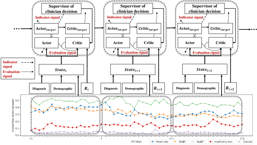
The above issues can be addressed by reinforcement learning for dynamic treatment regime (DTR) (Robins, 1986; Murphy, 2003). DTR is a sequence of tailored treatments according to the dynamic states of patients, which conforms to the clinical practice. As a real example shown in Figure 1, treatments for the patient vary dynamically over time with the accruing observations. The optimal DTR is determined by maximizing the evaluation signal which indicates the long-term outcome of patients, due to the delayed effect of the current treatment and the influence of future treatment choices (Chakraborty and Moodie, 2013). With the desired properties of dealing with delayed reward and inferring optimal policy based on non-optimal prescription behaviors, a set of reinforcement learning methods have been adapted to generate optimal DTR for life-threatening diseases, such as schizophrenia, non-small cell lung cancer, and sepsis (Shortreed and Moodie, 2012; Zhao et al., 2011; Nemati et al., 2016). Recently, some studies employ deep RL to solve the DTR problem based on large scale EHRs (Weng et al., 2017; Prasad et al., 2017; Raghu et al., 2017). Nevertheless, these methods may recommend treatments that are obviously different from doctors’ prescriptions due to the lack of the supervision from doctors, which may cause high risk (Mihatsch and Neuneier, 2002) in clinical practice. In addition, the existing methods are challenging for analyzing multiple diseases and the complex medication space.

In fact, the evaluation signal and indicator signal paly complementary roles (Barto, 2002; Clouse and Utgoff, 1992), where the indicator signal gives a basic effectiveness and the evaluation signal helps optimize policy. Imitation learning (Abbeel and Ng, 2004; Ratliff et al., 2006; Ziebart et al., 2008; Levine et al., 2011; Finn et al., 2016) utilizes the indicator signal to estimate a reward function for training robots by supposing the indicator signal is optimal, which is not in line with the clinical reality. Supervised actor-critic (Clouse and Utgoff, 1992; Benbrahim and Franklin, 1997; Barto, 2004) uses the indicator signal to pre-train a “guardian” and then combines “actor” output and “guardian” output to send low-risk actions for robots. However, the two types of signals are trained separately and cannot learn from each other. Inspired by these studies, we propose a novel deep architecture to generate recommendations for more general DTR involving multiple diseases and medications, called Supervised Reinforcement Learning with Recurrent Neural Network (SRL-RNN). The main novelty of SRL-RNN is to combine the evaluation signal and indicator signal at the same time to learn an integrated policy. More specifically, SRL-RNN consists of an off-policy actor-critic framework to learn complex relations among medications, diseases, and individual characteristics. The “actor” in the framework is not only influenced by the evaluation signal like traditional RL but also adjusted by the doctors’ behaviors to ensure safe actions. RNN is further adopted to capture the dependence of the longitudinal and temporal records of patients for the POMDP problem. Note that treatment and prescription are used interchangeably in this paper.

Our contributions can be summarized as follows:

• We propose a new deep architecture SRL-RNN for handling a more general DTR setting involving multiple diseases and medications. It learns the prescription policy by combing both the indicator signal and evaluation signal to avoid unacceptable risks and infer the optimal dynamic treatment.

• SRL-RNN applies an off-policy actor-critic framework to handle complex relations among multiple medications, diseases, and individual characteristics. The “actor” is adjusted by both the indicator signal and evaluation signal and RNN is further utilized to solve POMDP (see Section 4.4).

• Quantitative experiments and qualitative case studies on MIMIC-3 demonstrate that our method can not only reduce the estimated mortality in the hospital (see Section 5.2) by 4.4%, but also provide better medication recommendation.

The rest of this paper is organized as follows. We summarize the related work in Section 2 and provide necessary background knowledge in Section 3 for later introduction. In what follows, our model is specified in Section 4. Experimental results are presented in Section 5. Finally, we conclude our paper in Section 6.

2. Related Work

Early treatment recommendation systems heuristically map diseases into medications based on expert systems (Zhuo et al., 2016; Gunlicksstoessel et al., 2017; Almirall et al., 2012). Due to the difficulty of knowledge acquisition, it comes into data-driven approaches with two branches: supervised learning and reinforcement learning. In this section, we overview the related studies on data-driven treatment recommendation, and the methodologies of combing supervised learning and reinforcement learning.

Supervised learning for prescription focuses on minimizing the difference between recommended prescriptions and doctors’ prescriptions. Both Cheerla et al. (Cheerla and Gevaert, 2017) and Rosen et al. (Rosen-Zvi et al., 2008) proposed to utilize genomic information for recommending suitable treatments for patients with different diseases. However, genomic information is not widely spread and easy to acquire. In order to leverage massive EHRs to improve treatment recommendation, several pattern-based methods generate treatments by the similarity among patients (Zhang et al., 2014; Sun et al., 2016; Hu et al., 2016). Nevertheless, these methods are challenging to directly learn the relationship between patients and medications. Furthermore, it is challenging to calculate the similarities between patients’ complex longitudinal records. Recently, two deep models are proposed to learn a nonlinear mapping from diseases to drug categories based on EHRs, and achieve significant improvements. Bajor et al. (Bajor and Lasko, 2017) adopted a GRU model to predict the total medication categories given historical diagnosis records of patients. Zhang et al. (Zhang et al., 2017) proposed a deep model to not only learn the relations between multiple diseases and multiple medication categories, but also capture the dependence among medication categories. In addition, Wang et al. (Wang et al., 2018) utilized a trilinear model to integrate multi-source patient-specific information for personalized medicine.

A major concern for these SL-based prescription is that the behaviors of doctors are prone to be imperfect. Due to the knowledge gap and limited experiences of doctors, the ground truth of “good” treatment strategy is unclear in the medical literature (Marik, 2015). To address this issue, we prefer to use RL that is well-suited to infer optimal policies based on non-optimal prescriptions.

Reinforcement learning for prescription gives the treatments by maximizing the cumulated reward, where the reward can be assessment scores of disease or survival rates of patients. Daniel et al. (Susan M. Shortreed, 2011) employed tabular Q-learning to recommend medications for schizophrenia patients on real clinical data. Zhao et al. (Zhao et al., 2011) applied fitted Q-learning to discover optimal individualized medications for non-small cell lung cancer (NSCLC) based on simulation data, where a support vector regression (SVR) model is used to estimate Q-function. Nemati et al. (Nemati et al., 2016) leveraged a combination of Hidden Markov Models and deep Q-networks to predict optimal heparin dosing for patients in ICU under a POMDP environment. Applying these approaches to clinical practice is challenging for their use of relatively small amount of data. Most recently, based on large scale available EHRs, Weng et al. (Weng et al., 2017) combined sparse autoencoder and policy iteration to predict personalized optimal glycemic trajectories for severely ill septic patients, which reduces 6.3% mortality. Prasad et al. (Prasad et al., 2017) used Q-learning to predict personalized sedation dosage and ventilator support. Raghu et al. (Raghu et al., 2017) employed dual double deep Q-learning with continuous-state spaces to recommend optimal dosages of intravenous fluid and maximum vasopressor for sepsis.

However, without knowledgeable supervisors, the system may recommend treatments that are significantly different from doctors’, which may cause unacceptable risks (Mihatsch and Neuneier, 2002). Besides, these value based methods are hard to handle multiple diseases and complex medication space.

Methods of combing SL and RL utilize expert behaviors to accelerate reinforcement learning and avoid the risks of actions. Common examples are imitation learning (Abbeel and Ng, 2004; Ratliff et al., 2006; Ziebart et al., 2008; Levine et al., 2011; Finn et al., 2016) and supervised actor-critic (Clouse and Utgoff, 1992; Benbrahim and Franklin, 1997; Barto, 2004). Given the samples of expert trajectories, imitation learning requires th skill of estimating a reward function in which the reward of expert trajectories should enjoy the highest rewards. Recently, imitation learning combines deep learning to produce successful applications in robotics (Finn et al., 2016; Levine et al., 2016). However, these methods assume expert behaviors are optimal, which is not in line with clinical reality. Besides, most of them learn the policy based on the estimated reward function, instead of directly telling learners how to act. Supervised actor-critic uses the indicator signal to pre-train a “guardian”, and sends a low-risk action for robots by the weighted sum of “actor” output and “guardian” output, but each signal cannot learn from each other in the training process. Since this type of model requires much more expert behaviors, it has limited applications. In this paper, we focus on combining RL and SL by utilizing the large amount of doctors’ prescription behaviors. Our proposed model SRL-RNN is novel in that: (1) we train “actor” with the indicator signal and evaluation signal jointly instead of learning “guardian” and “actor” separately; (2) SRL-RNN combines an off-policy RL and classification based SL models, while supervised actor-critic combines an on-policy RL and regression based SL models; and (3) SRL-RNN enables capturing the dependence of longitudinal and temporal records of patients to solve the problem of POMDP.

3. Background

In this section, we give a definition of the Dynamic Treatment Regime (DTR) problem and an overview of preliminaries for our model. Some important notations mentioned in this paper are summarized in Table 1.

3.1. Problem Formulation

In this paper, DTR is modeled as a Markov decision process (MDP) with finite time steps and a deterministic policy consisting of an action space $\mathcal{A}$, a state space $\mathcal{S}$, and a reward function $r:\mathcal{S}\times\mathcal{A}\rightarrow\mathbb{R}$. At each time step $t$, a doctor observes the current state $s_{t}\in\mathcal{S}$ of a patient, chooses the medication $\hat{a}_{t}\in\{0,1\}^{K}$ from candidate set $\mathcal{A}$ based on an unknown policy $\hat{\mu}(s)$, and receives a reward $r_{t}$. Given the current observations of diseases, demographics, lab values, vital signs, and the output event of the patient which indicate the state $s_{t}$ , our goal is to learn a policy $\mu_{\theta}(s)$ to select an action (medication) $a_{t}$ by maximizing the sum of discounted rewards (return) from time step $t$, which is defined as $R_{t}=\sum_{i=t}^{T}\gamma^{(i-t)}r(s_{i},a_{i})$, and simultaneously minimizes the difference from clinician decisions $\hat{a}_{t}$.

There are two types of methods to learn the policy: the value-based RL learning a greedy policy $\mu(s)$ and the policy gradient RL maintaining a parameterized stochastic policy $\pi_{\theta}(a|s)$ or a deterministic policy $\mu_{\theta}(s)$ (see 3.2 for details), where $\theta$ is the parameter of the policy.

Figure 2. The general framework of supervised reinforcement learning with recurrent neural network. Solid arrows indicate the input diagnoses, demographics, rewards, clinician decisions timeseries variables, and historical states. Dashed arrows represent the indicator signal and evaluation signal to update the actor ($actor_{target}$) network and critic ($critic_{target}$) network.

Table 1. Important notations.

Notation	Description
$K$	the number of medications or medication categories
$\mathcal{A},a$	action space $\mathcal{A}\in\{0,1\}^{K}$, $a\in\mathcal{A},a_{k}\in\{0,1\}$ indicates whether the $k$-th medication is chosen for a patient
$\mathcal{S},s$	state space $\mathcal{S}$, $s\in\mathcal{S}$ consists of static demographic information, lab values, vital signs, etc.
$r$	reward function, if a patient survives, r=15, if the patient dies, r=-15 , and r=0 otherwise
$\gamma$	$\gamma\in[0,1]$ is a discount factor to balance the importance of immediate and future rewards
$\mu_{\theta}(s)$	deterministic policy learned from policy gradient
$\pi_{\theta}(a|s)$	stochastic policy learned from policy gradient
$\mu(s)$	a greedy policy learned from Q-learning
$\hat{\mu}(s)$	unknown policy of a doctor
$\beta(a|s)$	behavior policy, generate trajectories for off-policy learning
$Q^{\mu}(s,a)$, $Q^{\pi}(s,a)$	Q-values, the expected return at state $s$ after taking action $a$ following policy $\mu$ or $\pi$
$Q_{w}(s,a)$	estimated Q function
$V^{\mu_{\theta}}(s)$, $V^{\pi}(s)$	state value, the expected total discounted reward from state $s$
$\epsilon$	in $[0,1]$, the weighted parameter to balance RL and SL

3.2. Model Preliminaries

Q-learning (Watkins and Dayan, 1992) is an off-policy learning scheme that finds a greedy policy $\mu(s)=argmax_{a}Q^{\mu}(s,a)$, where $Q^{\mu}(s,a)$ denotes action-value or Q value and is used in a small discrete action space. For deterministic policy, the Q value can be calculated with dynamic programming as follows:

(1) $$Q^{\mu}(s_{t},a_{t})=\mathbb{E}_{r_{t},s_{t+1}\sim E}[r(s_{t},a_{t})+\gamma Q^{\mu}(s_{t+1},\mu_{t+1})],$$

where $E$ indicates the environment. Deep Q network (DQN) (Mnih et al., 2015) utilizes deep learning to estimate a non-linear Q function $Q_{w}(s,a)$ parameterized by $w$. The strategy of replay buffer is adopted to gain independent and identical distribution of samples for training. Moreover, DQN asynchronously updates a target network $Q_{w}^{tar}$ to minimize the least square loss as follows:

(2) $$\begin{split}L(w)=\mathbb{E}_{r_{t},s_{t}\sim E}[(Q_{w}(s_{t},a_{t})-y^{t})^{2}],\\ y^{t}=r(s_{t},a_{t})+\gamma Q_{w}^{tar}(s_{t+1},\mu(s_{t+1})).\end{split}$$

Policy gradient is employed to handle continuous or high dimensional actions. To estimate the parameter $\theta$ of $\pi_{\theta}$, we maximize the expected return from the start states $\mathbb{E}_{r_{i},s_{i}\sim\pi_{\theta}}[R_{1}]=\mathbb{E}_{r_{i},s_{i}\sim\pi_{\theta}}[V^{\pi_{\theta}}(s_{1})]$, which is reformulated as: $\mathbb{E}_{r_{i},s_{i}\sim\pi_{\theta}}[V^{\pi_{\theta}}(s_{1})]=J(\pi_{\theta})=\int_{\mathcal{S}}\rho^{\pi_{\theta}}(s)\int_{\mathcal{A}}\pi_{\theta}(a|s)r(s,a)\texttt{d}s\texttt{d}a$, where $V^{\pi_{\theta}}(s_{1})$ is the state value of the start state. $\rho^{\pi_{\theta}}(s^{\prime})=\int_{\mathcal{S}}\sum^{T}_{t=1}\gamma^{t-1}p_{1}(s)p(s\rightarrow s^{\prime},t,\pi_{\theta})\texttt{d}s$ is discounted state distribution, where $p_{1}(s_{1})$ is the initial state distribution and $p(s\rightarrow s^{\prime},t,\pi_{\theta})$ is the probability at state $s^{\prime}$ after transition of t time steps from state $s$. Policy gradient learns the parameter $\theta$ by the gradient $\nabla_{\theta}J(\pi_{\theta})$ which is calculated using the policy gradient theorem (Sutton et al., 2000):

(3) $$\begin{split}\nabla_{\theta}J(\pi_{\theta})=\int_{\mathcal{S}}\rho^{\pi_{\theta}}(s)\int_{\mathcal{A}}\nabla_{\theta}\pi_{\theta}(a|s)Q^{\pi_{\theta}}(s,a)\texttt{d}a\texttt{d}s\\ =\mathbb{E}_{s\sim\rho^{\pi\theta},a\in\pi_{\theta}}[\nabla_{\theta}log\pi_{\theta}(a|s)Q^{\pi_{\theta}}(s,a)],\end{split}$$

where the instantaneous reward $r(s,a)$ is replaced by the long-term value $Q^{\pi\theta}(s,a)$.

Actor-critic (Konda and Tsitsiklis, 2000) combines the advantages of Q-learning and policy gradient to achieve accelerated and stable learning. It consists of two components: (1) an actor to optimize the policy $\pi_{\theta}$ in the direction of gradient $\nabla_{\theta}J(\pi_{\theta})$ using Equation 3, and (2) a critic to estimate an action-value function $Q_{w}(s,a)$ with the parameter $w$ through Equation 2. Finally, we obtain the policy gradient denoted as $\nabla_{\theta}J(\pi_{\theta})=\mathbb{E}_{s\sim\rho^{\pi_{\theta}},a\in\pi_{\theta}}[\nabla_{\theta}log\pi_{\theta}(a|s)Q_{w}(s,a)]$.

In an off-policy setting, actor-critic estimates the value function of $\pi_{\theta}(a|s)$ by averaging the state distribution of behavior policy $\beta(a|s)$ (Degris et al., 2012). Instead of considering the stochastic policy $\pi_{\theta}(s|a)$, the deterministic policy gradient (DPG) theorem (Silver et al., 2014) proves that policy gradient framework can be extended to find deterministic off-policy $\mu_{\theta}(s)$, which is given as follows:

(4) $$\begin{split}\nabla_{\theta}J_{\beta}(\mu_{\theta})\approx\int_{s}\rho^{\beta}(s)\nabla_{\theta}\mu_{\theta}(s)Q^{\mu\theta}(s,a)\texttt{d}s\\ =\mathbb{E}_{s\sim\rho^{\beta}}[\nabla_{\theta}\mu_{\theta}(s)\nabla_{a}Q^{\mu\theta}(s,a)|_{a=\mu_{\theta}(s)}].\end{split}$$

Deep deterministic policy gradient (DDPG) (Lillicrap et al., 2015) adopts deep learning to learn the actor and critic in mini batches which store a replay buffer with tuples ($s_{t},a_{t},r_{t},s_{t+1}$). To ensure the stability of Q values, DDPG uses a similar idea as the target network of DQN to copy the actor and critic networks as $\mu_{\theta}^{tar}(s)$ and $Q^{tar}_{w}(s,a)$. Instead of directly copying the weights, DDPG uses a “soft” target update:

(5) $$\theta^{tar}\leftarrow\tau\theta+(1-\tau)\theta^{tar},~{}w^{tar}\leftarrow\tau w+(1-\tau)w^{tar},\quad\texttt{where}\quad\tau\ll 1.$$

4. SRL-RNN Architecture

This section begins with a brief overview of our approach. After that, we introduce the components of SRL-RNN and the learning algorithm in detail.

4.1. Overview

The goal of our task is to learn a policy $\mu_{\theta}(s)$ to recommend tailored treatments given the dynamic states of patients. SL learns the policy $\mu_{\theta}(s)$ by matching the indicator signals, which guarantees a standard and safe performance. But the “good” treatment strategy is unclear and the original goal of clinical decisions also tries to optimize the outcome of patients. RL learns the policy $\mu_{\theta}(s)$ by maximizing evaluation signals in a sequential dynamic system which reflects the clinical facts and can infer the optimal policy based on non-optimal strategies. But without supervision, RL may produce unacceptable medications which give high risk. Intuitively, the indicator signal and evaluation signal play complementary roles (demonstrated in Section 5.4). Thus, SRL-RNN is proposed to combine these two signals at the same time, where the cumulated reward $r_{t}$ is the evaluation signal and the prescription $\hat{a}_{t}$ of doctors from the unknown policy $\hat{\mu}(s)$ is the indicator signal.

Figure 2 shows our proposed supervised reinforcement learning architecture (SRL-RNN), which consists of three core networks: Actor ($Actor_{target}$), Critic ($Critic_{target}$), and LSTM. The actor network recommends the time-varying medications according to the dynamic states of patients, where a supervisor of doctors’ decisions provides the indicator signal to ensure safe actions and leverages the knowledge of doctors to accelerate learning process. The critic network estimates the action value associated with the actor network to encourage or discourage the recommended treatments. Due to the lack of fully observed states in the real world, LSTM is used to extend SRL-RNN to handle POMDP by summarizing the entire historical observations to capture a more complete observations.

4.2. Actor Network Update

The actor network learns a policy $\mu_{\theta}(s)$ parameterized by $\theta$ to predict the time-varying treatments for patients, where the input is $s_{t}$ and the output is the prescription $a_{t}$ recommended by $\mu_{\theta}(s)$. We employ reinforcement learning and supervised learning to optimize the parameter $\theta$ jointly. By combining the two learning tasks together, we maximize the following objective function:

(6) $$\begin{split}J(\theta)=(1-\epsilon)J_{RL}(\theta)+\epsilon(-J_{SL}(\theta)),\end{split}$$

where $J_{RL}(\theta)$ is the objective function of RL task (in Equation 8) which tries to maximize the expected return, $J_{SL}(\theta)$ is the objective function of SL task (in Equation 10) which tries to minimize the difference from doctors’ prescriptions, and $\epsilon$ is a weight parameter to trade off the reinforcement learning and supervised learning tasks. Intuitively, our objective function aims to predicting mediations which give both high expected returns and low errors. Mathematically, the parameter $\theta$ of the learned policy is updated by gradient ascent as follows:

(7) $$\theta=\theta+\alpha((1-\epsilon)\nabla J_{RL}(\theta)+\epsilon(-\nabla J_{SL}(\theta))),$$

where $\alpha\in[0,1]$ is a positive learning rate, and $\nabla J_{RL}(\theta)$ and $\nabla J_{SL}(\theta)$ are acquired by the RL and SL tasks, respectively.

For the reinforcement learning task, we seek to learn the policy $\mu_{\theta}(s)$ by maximizing the state value of $\mu_{\theta}(s)$ averaging over the state distribution of the behaviors of doctors:

(8) $$\begin{split}J_{RL}(\theta)=\mathbb{E}_{s\sim\rho^{\hat{\mu}(s)}}[V^{\mu_{\theta}}(s)]=\mathbb{E}_{s\sim\rho^{\hat{\mu}(s)}}[Q_{w}(s,\mu_{\theta}(s))].\end{split}$$

Let the parameter $\theta$ in RL task be the weights of a neural network. $\theta$ is updated by gradient ascent, $\theta^{t+1}=\theta^{t}+\alpha(1-\epsilon)\nabla J_{RL}(\theta^{t})$, where $\nabla J_{RL}(\theta^{t})$ is calculated by the deterministic off-policy gradient using Equation 4:

(9) $$\begin{split}\nabla J_{RL}(\theta^{t})\approx\mathbb{E}_{s_{t}\sim\rho^{\hat{\mu}(s)}}[\nabla_{\theta}\mu_{\theta}(s)|_{s=s_{t}}\nabla_{a}Q_{w}(s,a)|_{s=s_{t},a=\mu_{\theta}(s_{t})}].\end{split}$$

Let $a_{t}$ be the treatment recommended by $\mu_{\theta}(s_{t})$. $\nabla_{a}Q_{w}(s,a)$ is obtained by the chain rule, which is used to tell the medications predicted by the actor are “good” or “bad”. When the gradient $\nabla_{a}Q_{w}(s_{t},a_{t})$ is positive, the policy $\mu_{\theta}(s)$ will be pushed to be closer to $a_{t}$. Otherwise, $\mu_{\theta}(s)$ will be pushed away from $a_{t}$. $\nabla_{\theta}\mu_{\theta}(s)$ is a Jacobian matrix where each column is the gradient $\nabla_{\theta}[\mu_{\theta}(s)]_{k}$ of $k$-th medication of $\mu_{\theta}(s)$ with respect to $\theta$.

For the supervised learning task, we try to learn the policy $\mu_{\theta}(s)$ through minimizing the difference between treatments predicted by $\mu_{\theta}(s)$ and prescriptions given from the doctor’s policy $\hat{\mu}(s)$, using the cross entropy loss:

(10) $$\begin{split}J_{SL}({\theta^{t}})=\mathbb{E}_{s\sim\rho^{\hat{\mu}(s)}}[-\frac{1}{K}\sum^{K}_{k=1}\hat{a}_{t,k}log\mu_{\theta}^{k}(s)+\\ (1-\hat{a}_{t,k})log(1-\mu_{\theta}^{k}(s)]|_{s=s_{t}},\end{split}$$

where $K$ indicates the number of medications or medication categories, and $\hat{a}_{t,k}\in\{0,1\}$ denotes whether the doctor chooses $k$-th medication at time step $t$ and $\mu_{\theta}^{k}(s)$ is the probability of the $k$-th medication predicted by $\mu_{\theta}(s)$. The parameter $\theta$ in SL task is updated by the gradient descent $\theta^{t+1}=\theta^{t}-\alpha\epsilon\nabla J_{SL}(\theta^{t})$ where $\nabla J_{SL}(\theta^{t})$ is derived by the chain rule as follows:

(11) $$\nabla J_{SL}(\theta^{t})=\mathbb{E}_{s\sim\rho^{\hat{\mu}(s)}}[-\phi\nabla_{\theta}\mu_{\theta}(s|\theta^{t})|_{s=s_{t}}],$$

where $\phi=\frac{1}{K}\sum^{K}_{k=1}\frac{\hat{a}_{t,k}-{a}_{t,k}^{SL}}{(1-{a}_{t,k}^{SL}){a}_{t,k}^{SL}}$. Substituting Equation 9 and Equation 11 into Equation 7 gives the final actor update:

(12) $$\begin{split}\theta=\theta+\alpha[(1-\epsilon)\nabla_{a}Q_{w}(s,a)|_{s=s_{t},a=\mu_{\theta}(s_{t})}+\epsilon\phi]\nabla_{\theta}\mu_{\theta}(s)|_{s=s_{t}}.\end{split}$$

The above formulas show that we can use $\epsilon$ to trade off the RL and SL tasks, where $\epsilon$ is a hyper parameter in this paper and the effect of $\epsilon$ is shown in Figure 6.

4.3. Critic Network Update

The critic network is jointly learned with the actor network, where the inputs are the states of patients, doctor prescriptions, actor outputs, and rewards. We can do this due to the critic network is only needed for guiding the actor during training, while only the actor network is required at test time. The critic network uses a neural network to learn the action-value function $Q_{w}(s,a)$ which is used to update the parameters of the actor in the direction of performance improvement $\nabla_{a}Q_{w}(s,a)$. The output of the critic network is the Q value $Q(s_{t},a_{t})$ of state $s_{t}$ after taking action $a_{t}$, where $Q(s_{t},a_{t})$ is predicted by the Q-function $Q_{w}(s,a)$.

The update formula for parameter $w$ of $Q_{w}(s,a)$ is similar to DQN which is specified in Equation 1 and 2:

(13) $$\begin{split}J(w)=\mathbb{E}_{r_{t},s_{t}\sim\rho^{\hat{\mu}(s)}}[(Q_{w}(s_{t},\hat{a}_{t})-y^{t})^{2}]\\ y^{t}=r(s_{t},\hat{a}_{t})+\gamma Q_{w}^{tar}(s_{t+1},\mu_{\theta}(s_{t+1})),\end{split}$$

where $\mu_{t+1}(s_{t+1})$ are the medications recommend by the actor network. $w$ is updated by the gradient descent:

(14) $$w=w-\alpha_{Q}(Q_{w}(s_{t},\hat{a}_{t})-y^{t})\nabla_{w}Q_{w}(s_{t},a_{t}),$$

where $\delta=(Q_{w}(s_{t},\hat{a}_{t})-y^{t})$ is called Temporal Difference (TD) error which is used for learning the Q-function.

4.4. Recurrent SRL

In the previous section, we assume the state $s_{t}$ of a patient is fully observed. In fact, we are always unable to obtain the full states of the patient. Here we reformulate the environment of SRL-RNN as POMDP. POMDP can be described as a 4-tuple ($\mathcal{S},\mathcal{A},\mathcal{R},\mathcal{O}$), where $\mathcal{O}$ are observations. We obtain the observation $o\in\mathcal{O}$ directly which conditions on $p(o_{t}|s_{t})$, with the not fully observable state $s_{t}$. LSTM has been verified to improve performance on POMDP by summarizing entire historical observations $c_{t}=f(o_{1},o_{2},...,o_{t})$ when using policy gradient (Wierstra et al., 2007) and Q-learning (Hausknecht and Stone, 2015). In LSTM, the hidden units ${c}_{t}$ is to encapsulate the entire observation history $o_{1:t}$. In order to capture the dependence of the longitudinal and temporal records of the patient, we employ a LSTM with SRL to represent historical observation $c_{t}$ for a more complete observation.

The updates of the parameters of actor network and critic network are modified as follows:

(15) $$\begin{split}\theta=\theta+\alpha\sum_{t}([(1-\epsilon)\nabla_{a}Q_{w}(c,a)|_{c=c_{t},a=\mu_{\theta}(c_{t})}\\ +\epsilon\phi]\nabla_{\theta}\mu_{\theta}(c)|_{c=c_{t}}),\end{split}$$

(16) $$w=w-\alpha\sum_{t}(Q_{w}(c_{t},\hat{a}_{t})-y^{t})\nabla_{w}Q_{w}(c_{t},a_{t}).$$

4.5. Algorithm

Putting all the aforementioned components together, the learning algorithm of SRL-RNN is provided below.

Algorithm 1 SRL-RNN

0:  observations $O$, actions $A$, reward function $r$, # of epochs $N$, weight parameter $\epsilon$, # of medications $K$;

1:  Store sequences ($o_{1},a_{1},r_{1},...,o_{T},a_{T},r_{T}$) in buffer D;

2:  Initialize actor $\mu_{\theta}(c)$, target actor $\mu_{\theta}(c)^{tar}$, critic $Q_{w}(c,a)$, target critic $Q_{w}(c,a)^{tar}$, and TD error $\delta=0$;

3:  for $n=0$ to $N$ do

4:     Sample ($o_{1}^{i},a_{1}^{i},r_{1}^{i},...,o_{T}^{i},a_{T}^{i},r_{T}^{i}$) $i=1,..,I$ from D;

5:     $c_{t}^{i}\leftarrow f(o_{1}^{i},o_{2}^{i},...,o_{t}^{i})$ given by LSTM

6:     $y_{t}^{i}\leftarrow r_{t}^{i}+\gamma Q^{tar}_{w}(c_{t}^{i+1},\mu_{\theta}^{tar}(c_{t}^{i+1}))$

7:     ${a}_{t}^{i}\leftarrow$ action given by $\mu_{\theta}(c_{t}^{i})$

8:     $\hat{a}_{t}^{i}\leftarrow$ action given by doctor $\hat{\mu}(c_{t}^{i})$

9:     $\delta_{t}^{i}\leftarrow Q_{w}(c_{t}^{i},\hat{a}_{t}^{i})-y_{t}^{i}$

10:     $w\leftarrow w+\alpha\frac{1}{IT}\sum_{i}\sum_{t}\delta_{t}^{i}\nabla_{w}Q_{w}(c_{t}^{i},a_{t}^{i})$ $\vartriangleright$ update critic

11:     $w^{tar}\leftarrow\tau w+(1-\tau)w^{tar}$ $\vartriangleright$ update target critic

12:     $\nabla_{a}Q_{w}(c_{t}^{i},{a}_{t}^{i})\leftarrow$ given by $Q_{w}(c_{t}^{i},a_{t}^{i})$

13:     $\eta_{t}^{i}\leftarrow\frac{1}{K}\sum^{K}_{k=1}\frac{\hat{a}_{t,k}^{i}-{a}_{t,k}^{i}}{(1-{a}_{t,k}^{i}){a}_{t,k}^{i}}$

14:     $\theta\leftarrow\theta+\alpha\frac{1}{IT}\sum_{i}\sum_{t}[(1-\epsilon)\nabla_{a}Q_{w}(c_{t}^{i},a_{t}^{i})+\epsilon\eta_{t}^{i}]$$\nabla_{\theta}\mu_{\theta}(c_{t}^{i})$ $\vartriangleright$ update actor

15:     $\theta^{tar}\leftarrow\tau\theta+(1-\tau)\theta^{tar}$$\vartriangleright$ update target actor

16:  end for

5. Experiments

In this section, we present the quantitative and qualitative experiment results on MIMIC-3.

5.1. Dataset and Cohort

The experiments are conducted on a large and publicly available dataset, namely the Multiparameter Intelligent Monitoring in Intensive Care (MIMIC-3 v1.4) database (Johnson et al., 2016). MIMIC-3 encompasses a very large population of patients compared to other public EHRs. It contains hospital admissions of 43K patients in critical care units during 2001 and 2012, involving 6,695 distinct diseases and 4,127 drugs. To ensure statistical significance, we extract the top 1,000 medications and top 2,000 diseases (represented by ICD-9 codes) which cover 85.4% of all medication records and 95.3% of all diagnosis records, respectively. In order to experiment on different granularity of medications, we map the 1,000 medications into the third level of ATC (medication codes) using a public tool, resulting 180 distinct ATC codes. Therefore, the action space size of the experiments is 1,000 exact medications ($K=1000$) or 180 drug categories ($K=180$).

For each patient, we extract relevant physiological parameters with the suggestion of clinicians, which include static variables and time-series variables. The static variables cover eight kinds of demographics: gender, age, weight, height, religion, language, marital status, and ethnicity. The time-series variables contain lab values, vital signs, and output events, such as diastolic blood pressure, fraction of inspiration O2, Glascow coma scale, blood glucose, systolic blood pressure, heart rate, pH, respiratory rate, blood oxygen saturation, body temperature, and urine output. These features correspond to the state $s$ in MDP or the observation $o$ in POMDP. We impute the missing variable with k-nearest neighbors and remove admissions with more than 10 missing variables. Each hospital admission of a patient is regarded as a treatment plan. Time-series data in each treatment plan is divided into different units, each of which is set to 24 hours since it is the median of the prescription frequency in MIMIC-3. If several data points are in one unit, we use their average values instead. Following (Weng et al., 2017), we remove patients less than 18 years old because of the special conditions of minors. Finally, we obtain 22,865 hospital admissions, and randomly divide the dataset for training, validation, and testing sets by the proportion of 80/10/10.

5.2. Evaluation Metrics

Evaluation methodology in treatment recommendation is still a chanllenge. Thus we try all evaluation metrics used in state-of-art methods to judge our model.

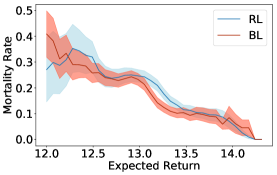
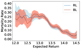
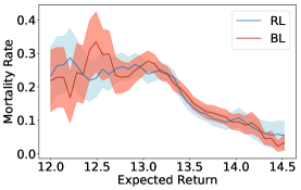
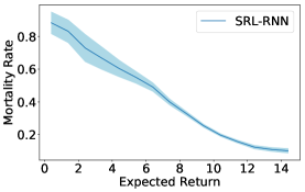
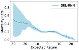
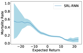
Following (Weng et al., 2017; Raghu et al., 2017), we use the estimated in-hospital mortality rates to measure whether policies would eventually reduce the patient mortality or not. Specifically, we discretize the learned Q-values of each test example into different units with small intervals shown in the x-axis of Figure 3. Given an example denoting an admission of a patient, if the patient died in hospital, all the Q-values belonging to this admission are associated with a value of 1 as mortality and the corresponding units add up these values. After scanning all test examples, the average estimated mortality rates for each unit are calculated, shown in y-axis of Figure 3. Based on these results, the mortality rates corresponding to the expected Q-values of different policies are used as the measurements to denote the estimated in-hospital mortality (see details in (Weng et al., 2017; Raghu et al., 2017)). Although the estimated mortality does not equal the mortality in real clinical setting, it is a universal metric currently for computational testing.

Inspired by (Zhang et al., 2017), we further utilize mean Jaccard coefficient to measure the degree of consistency between prescriptions generated by different methods and those from doctors. For a patient $p_{i}$ in the $t$-th day of ICU, let $\hat{U}_{t}^{i}$ be the medication set given by doctors and $U_{t}^{i}$ be the medication set recommended from learned policies. The mean Jaccard is defined as $\frac{1}{M}\sum_{i=1}^{M}\frac{1}{T_{i}}\sum_{t=1}^{T_{i}}\frac{\mid U_{t}^{i}\cap\hat{U}_{t}^{i}\mid}{\mid U_{t}^{i}\cup\hat{U}_{t}^{i}\mid}$, where $M$ is the number of patients and $T_{i}$ is the number of ICU days for the patient $p_{i}$.

5.3. Comparison Methods

All the adopted baselines models in the experiments are as follows, where BL, RL, and SD3Q are the alternatives of SRL-RNN we proposed.

• Popularity-20 (POP-20): POP-20 is a patten-based method, which chooses the top-K most co-occurring medications with the target diseases as prescriptions. We set $K=20$ for its best performance on the validation dataset.

• Basic-LSTM (BL): BL uses LSTM to recommend the sequential medications based on the longitudinal and temporal records of patients. Inspired by Doctor-AI (Choi et al., 2016), BL fuses multi-sources of patient-specific information and considers each admission of a patient as a sequential treatment to satisfy the DTR setting. BL consists of a 1-layer MLP (M-1) to model diseases, a 1-layer MLP (M-2) to model static variables, and a 1-layer LSTM sequential model (L-1) to capture the time-series variables. These outputs are finally concatenated to predict prescriptions at each time-step.

• Reward-LSTM (RL): RL has the same framework as BL, except that it considers another signal, i.e., feedback of mortality, to learn a nontrivial policy. The model involves three steps: (1) clustering the continuous states into discrete states, (2) learning the $Q$-values using tabular Q-learning, (3) and training the model by simultaneously mimicking medications generated by doctors and maximizing cumulated reward of the policy.

• Dueling Double-Deep Q learning (D3Q) (Raghu et al., 2017): D3Q is a reinforcement learning method which combines dueling Q, double Q, and deep Q together. D3Q regards a treatment plan as DTR.

• Supervised Dueling Double-Deep Q (SD3Q): Instead of separately learning the Q-values and policy as RL, SD3Q learns them jointly. SD3Q involves a D3Q architecture, where supervised learning is additionally adopted to revise the value function.

• Supervised Actor Critic (SAC) (Clouse and Utgoff, 1992): SAC uses the indicator signal to pre-train a “guardian” and then combines “actor” output and “guardian” output to send low-risk actions for robots. We transform it into a deep model for a fair comparison.

• LEAP (Zhang et al., 2017): LEAP leverages a MLP framework to train a multi-label model with the consideration of the dependence among medications. LEAP takes multiple diseases as input and multiple medications as output. Instead of considering each admission as a sequential treatment process, LEAP regards each admission as a static treatment setting. We aggregate the multiple prescriptions recommended by SRL-RNN as SRL-RNN (agg) for a fair comparison.

• LG (Bajor and Lasko, 2017): LG takes diseases as input and adopts a 3-layer GRU model to predict the multiple medications.

Table 2. Performance comparison on test sets for prescription prediction. l-3 ATC indicates the third level of ATC code and Medications indicates the exact drugs.

	Estimated Mortality		Jaccard
Granularity	l-3 ATC	Medications	l-3 ATC	Medications
Dynamic treatment setting
LG	0.226	0.235	0.436	0.356
BL	0.217	0.221	0.512	0.376
RL	0.209	0.213	0.524	0.378
D3Q	0.203	0.212	0.109	0.064
SD3Q	0.198	0.201	0.206	0.143
SAC	0.196	0.202	0.517	0.363
SRL-RNN	0.153	0.157	0.563	0.409
Static treatment setting
POP-20	0.233	0.247	0.382	0.263
LEAP	0.224	0.229	0.495	0.364
SRL-RNN (agg)	0.153	0.157	0.579	0.426

5.4. Result Analysis

(a) all-demo-disease

(b) all-demo

(c) all

(d) all-demo-disease

(e) all-demo

(f) all

Figure 3. Mortality-expected-return curve computed by the learned policies.

Model comparisons. Table 2 depicts the mortality rates and Jaccard scores for all the adopted models on MIMIC-3. By first comparing the results of LG, BL, and RL, we find that RL outperforms both BL and LG, showing that incorporating the evaluation signal into supervised learning can indeed improve the results. We then compare SD3Q with its simplified version D3Q. The better performance of SD3Q indicates the knowledgeable supervision guarantees a standard performance of the learned policy. In the static treatment setting, LEAP improves the basic method POP-20 by a large margin, which demonstrates that capturing the relations between multiple diseases and multiple medications is beneficial for better prescriptions.

Finally, our proposed model SRL-RNN performs significantly better than all the adopted baselines, both in the dynamic treatment setting and static treatment setting. The reasons are: 1) SRL-RNN regards the treatment recommendation as a sequential decision process, reflecting the clinical practice (compared with LEAP and POP-20), and utilizes evaluation signal to infer an optimal treatment (compared with LG and BL); 2) SRL-RNN considers the prescriptions of doctors as supervision information to learn a robust policy (compared with D3Q), and applies the off-policy actor-critic framework to handle complex relations of medications, diseases, and individual characteristics (compared with SD3Q); 3) SRL-RNN integrates supervised learning and reinforcement learning in an end-to-end learning fashion for sharing the information between evaluation signal and indicator signal (compared with RL and SAC); and 4) SRL-RNN adopts RNN to solve POMDP by obtaining the representations of the entire historical observations.

Ablation study. The different contributions of the three types of features are reported in this part. To be specific, we progressively add the patient-specific information, i.e., time series variables, diseases, and demographics, into the selected models. As shown in Table 3, the Jaccard scores of the three methods monotonically increase. In addition, the estimated mortality rates of SRL-RNN monotonically decrease. However, the estimated mortality variations of BL and RL are not the same as that of SLR-RNN. It might be due to the fact that with constant Q-values learned by tabular Q-learning, learning a robust policy is a little hard.

Table 3. Ablation study of the features. all indicates all the features: demographic, diseases and time-series variables. The symbol “-” stands for “subtracting”.

Method	Feature	Estimated Mortality	Jaccard
BL	all-demo-disease	0.242	0.323
	all-demo	0.212	0.360
	all	0.221	0.376
RL	all-demo-disease	0.184	0.332
	all-demo	0.203	0.371
	all	0.213	0.378
SRL-RNN	all-demo-disease	0.173	0.362
	all-demo	0.162	0.403
	all	0.157	0.409

Effectiveness and stability of policy. The relations between expected returns and mortality rates are shown in Figure 3. We observe SRL-RNN has a more clear negative correlation between expected returns and mortality rates than BL and RL. The reason might be that BL ignores the evaluation signal while RL discretizes the continuous states, incurring information loss.

Figure 4. Comparison of how observed mortality rates (y-axis) vary with the difference between the prescriptions generated by the optimal policy and the prescriptions administered by doctors (x-axis).

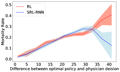
Figure 4 shows how the observed mortality changes with the difference between the learned policies (by RL and SRL-RNN) and doctors’ prescriptions. Let $D_{t}^{i}$ be the treatment difference for patient $p_{i}$ in the $t$-th day, and $K$ is the number of candidate classes of medications. We calculate the difference by $D_{t}^{i}=\sum_{k=1}^{K}{\mid U_{t,k}^{i}-\hat{U}_{t,k}^{i}\mid}$. When the difference is minimum, we obtain the lowest mortality rates of 0.021 and 0.016 for RL and SRL-RNN, respectively. This phenomenon shows that SRL-RNN and RL can both learn good policies while SRL-RNN slightly outperforms RL for its lower mortality rate.

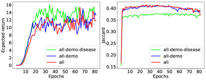
Figure 5 presents the expected return and Jaccard scores obtained in each learning epoch of SRL-RNN with different features. Notably, SRL-RNN is able to combine reinforcement learning and supervised learning to obtain the optimal policy in a stable manner. We can see Jaccard is learned faster than Q-values, indicating that leaning Q-values might need rich trajectories.

Figure 5. Expected return and Jaccard in different learning epochs with different features.

Case studies. Table 4 shows the prescriptions generated by different models for two patients in different ICU days. For the first patient who is finally dead, LG recommends much more medications which seem to be non-informative. LEAP generates the same medications for patients in different ICU days, without considering the change of patient states. An interesting observation is that the prescriptions recommended by SRL-RNN are much different from doctors’, especially for the stronger tranquilizers such as Acetaminophen and Morphine Sulfate. Actually, for an ICU patient with a severe trauma, it is important to give full sedation in early treatment. Considering the second surviving patient, the similarity between the prescriptions of SRL-RNN and doctor becomes larger, indicating the rationality of SRL-RNN. Particularly, all the models except SRL-RNN recommend redundant medications in different days, while the prescriptions of doctors are significantly different.

Figure 6. The effect of $\epsilon$.

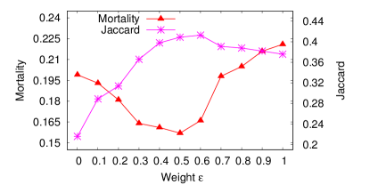
Effect of $\epsilon$. Figure 6 shows the effectiveness of the weight parameter $\epsilon$ in Equation 12, which is used to balance RL and SL. It achieves the highest Jaccard scores and lowest mortality rates when taking the values of 0.5 and 0.6, which verifies that SRL-RNN can not only significantly reduce the estimated mortality but also recommend better medications as well.

6. Conclusion

In this paper, we propose the novel Supervised Reinforcement Learning with Recurrent Neural Network (SRL-RNN) model for DTR, which combines the indicator signal and evaluation signal through the joint supervised and reinforcement learning. SRL-RNN incorporates the off-policy actor-critic architecture to discover optimal dynamic treatments and further adopts RNN to solve the POMDP problem. The comprehensive experiments on the real world EHR dataset demonstrate SRL-RNN can reduce the estimated mortality in hospital by up to 4.4% and provide better medication recommendation as well.

Table 4. Case study of prescription recommendation.

Diagnosis	day	method	treatment
Traumatic brain hemorrhage, Spleen injury, intrathoracic injury, Contusion of lung, motor vehicle traffic collision, Acute posthemorrhagic anemia	1	Doctor	Potassium Chloride, Magnesium Sulfate, Calcium Gluconate, Phytonadione, Famotidine, Mannitol
		LG	Potassium Chloride, Acetaminophen,Morphine Sulfate,Docusate Sodium, Bisacodyl, Magnesium Sulfate, Calcium Gluconate, Fentanyl Citrate, Famotidine, Potassium Chloride
		LEAP	Potassium Chloride, Acetaminophen, Heparin, Magnesium Sulfate,Calcium Gluconate, Fentanyl Citrate, Famotidine
		SRL-RNN	Potassium Chloride, Acetaminophen, Morphine Sulfate, Magnesium Sulfate, Calcium Gluconate, Fentanyl Citrate, Famotidine
	2	Doctor	Potassium Chloride, Acetaminophen, Magnesium Sulfate, Calcium Gluconate, Fentanyl Citrate, Famotidine
		LG	Acetaminophen, Morphine Sulfate, Heparin, Docusate Sodium, Bisacodyl, Senna, Oxycodone-Acetaminophen, Ondansetron, Famotidine
		LEAP	Potassium Chloride, Acetaminophen, Heparin, Magnesium Sulfate, Calcium Gluconate, Fentanyl Citrate, Famotidine
		SRL-RNN	Potassium Chloride, Acetaminophen, Morphine Sulfate, Magnesium Sulfate, Calcium Gluconate, Fentanyl Citrate, Propofol
Coronary atherosclerosis, pleural effusion, Percutaneous coronary angioplasty, Hypopotassemia, pericardium, Personal history of malignant neoplasm	1	Doctor	Acetaminophen, Morphine Sulfate, Lorazepam, Heparin, Docusate Sodium, Aspirin EC, Zolpidem Tartrate, Amlodipine, Pravastatin
		LG	Acetaminophen, Metoprolol, Morphine Sulfate, Heparin, Magnesium Sulfate, Senna, Aspirin, Pantoprazole, Lisinopril, Atorvastatin, Docusate Sodium, Clopidogrel Bisulfate, Atropine Sulfate, Potassium Chloride
		LEAP	Acetaminophen, Heparin, Docusate Sodium, Magnesium Sulfate, Potassium Chloride, Acetaminophen
		SRL-RNN	Acetaminophen, Morphine Sulfate, Lorazepam, Aspirin EC, Docusate Sodium, Pravastatin, Heparin Sodium, Zolpidem Tartrate,
	2	Doctor	Potassium Chloride
		LG	Acetaminophen, Morphine Sulfate, Heparin, Magnesium Sulfate, Senna, Aspirin, Pantoprazole, Lisinopril, Atorvastatin, Docusate Sodium, Clopidogrel Bisulfate, Atropine Sulfate, Potassium Chloride
		LEAP	Acetaminophen, Heparin, Docusate Sodium, Magnesium Sulfate, Potassium Chloride, Acetaminophen
		SRL-RNN	Potassium Chloride, Calcium Gluconate, Docusate Sodium

References

- (1)
- Abbeel and Ng (2004) Pieter Abbeel and Andrew Y Ng. 2004. Apprenticeship learning via inverse reinforcement learning. In ICML. ACM, 1.
- Almirall et al. (2012) D Almirall, S. N. Compton, M Gunlicks-Stoessel, N. Duan, and S. A. Murphy. 2012. Designing a pilot sequential multiple assignment randomized trial for developing an adaptive treatment strategy. Statistics in Medicine (2012), 1887–902.
- Bajor and Lasko (2017) Jacek M Bajor and Thomas A Lasko. 2017. Predicting Medications from Diagnostic Codes with Recurrent Neural Networks. ICLR (2017).
- Barto (2002) Andrew G Barto. 2002. Reinforcement Learning in Motor Control. In The handbook of brain theory and neural networks.
- Barto (2004) MTRAG Barto. 2004. supervised actor-critic reinforcement learning. Handbook of learning and approximate dynamic programming (2004), 359.
- Benbrahim and Franklin (1997) Hamid Benbrahim and Judy A Franklin. 1997. Biped dynamic walking using reinforcement learning. Robotics and Autonomous Systems (1997), 283–302.
- Chakraborty and Moodie (2013) Bibhas Chakraborty and EE Moodie. 2013. Statistical methods for dynamic treatment regimes. Springer.
- Cheerla and Gevaert (2017) N Cheerla and O Gevaert. 2017. MicroRNA based Pan-Cancer Diagnosis and Treatment Recommendation:. Bmc Bioinformatics (2017), 32.
- Choi et al. (2016) Edward Choi, Mohammad Taha Bahadori, Andy Schuetz, Walter F. Stewart, and Jimeng Sun. 2016. Doctor AI: Predicting Clinical Events via Recurrent Neural Networks. In Proceedings of the 1st Machine Learning for Healthcare Conference. PMLR, 301–318.
- Clouse and Utgoff (1992) Jeffery A. Clouse and Paul E. Utgoff. 1992. A Teaching Method for Reinforcement Learning. In International Workshop on Machine Learning. 92–110.
- Degris et al. (2012) Thomas Degris, Patrick M Pilarski, and Richard S Sutton. 2012. Model-free reinforcement learning with continuous action in practice. In American Control Conference (ACC). IEEE, 2177–2182.
- Finn et al. (2016) Chelsea Finn, Sergey Levine, and Pieter Abbeel. 2016. Guided cost learning: Deep inverse optimal control via policy optimization. In ICML. 49–58.
- Gunlicksstoessel et al. (2017) M Gunlicksstoessel, L Mufson, A Westervelt, D Almirall, and S Murphy. 2017. A Pilot SMART for Developing an Adaptive Treatment Strategy for Adolescent Depression. J Clin Child Adolesc Psychol (2017), 1–15.
- Hausknecht and Stone (2015) Matthew Hausknecht and Peter Stone. 2015. Deep recurrent q-learning for partially observable mdps. CoRR, abs/1507.06527 (2015).
- Hu et al. (2016) Jianying Hu, Adam Perer, and Fei Wang. 2016. Data driven analytics for personalized healthcare. In Healthcare Information Management Systems. 529–554.
- Johnson et al. (2016) Alistair EW Johnson, Tom J Pollard, Lu Shen, et al. 2016. MIMIC-III, a freely accessible critical care database. Scientific data (2016).
- Konda and Tsitsiklis (2000) Vijay R Konda and John N Tsitsiklis. 2000. Actor-critic algorithms. In NIPS. 1008–1014.
- Levine et al. (2016) Sergey Levine, Chelsea Finn, Trevor Darrell, and Pieter Abbeel. 2016. End-to-end training of deep visuomotor policies. JMLR (2016), 1–40.
- Levine et al. (2011) Sergey Levine, Zoran Popovic, and Vladlen Koltun. 2011. Nonlinear inverse reinforcement learning with gaussian processes. In NIPS. 19–27.
- Lillicrap et al. (2015) Timothy P Lillicrap, Jonathan J Hunt, Alexander Pritzel, Nicolas Heess, Tom Erez, Yuval Tassa, David Silver, and Daan Wierstra. 2015. Continuous control with deep reinforcement learning. arXiv preprint arXiv:1509.02971 (2015).
- Marik (2015) P. E. Marik. 2015. The demise of early goal-directed therapy for severe sepsis and septic shock. Acta Anaesthesiologica Scandinavica (2015), 561.
- Mihatsch and Neuneier (2002) Oliver Mihatsch and Ralph Neuneier. 2002. Risk-sensitive reinforcement learning. Machine learning (2002), 267–290.
- Mnih et al. (2015) Volodymyr Mnih, Koray Kavukcuoglu, David Silver, et al. 2015. Human-level control through deep reinforcement learning. Nature (2015), 529–533.
- Murphy (2003) Susan A Murphy. 2003. Optimal dynamic treatment regimes. Journal of the Royal Statistical Society: Series B (Statistical Methodology) 65, 2 (2003), 331–355.
- Nemati et al. (2016) Shamim Nemati, Mohammad M. Ghassemi, and Gari D. Clifford. 2016. Optimal medication dosing from suboptimal clinical examples: A deep reinforcement learning approach. In Engineering in Medicine and Biology Society. 2978.
- Prasad et al. (2017) Niranjani Prasad, Li Fang Cheng, Corey Chivers, Michael Draugelis, and Barbara E Engelhardt. 2017. A Reinforcement Learning Approach to Weaning of Mechanical Ventilation in Intensive Care Units. (2017).
- Raghu et al. (2017) Aniruddh Raghu, Matthieu Komorowski, Imran Ahmed, Leo Celi, Peter Szolovits, and Marzyeh Ghassemi. 2017. Deep Reinforcement Learning for Sepsis Treatment. arXiv preprint arXiv:1711.09602 (2017).
- Ratliff et al. (2006) Nathan D Ratliff, J Andrew Bagnell, and Martin A Zinkevich. 2006. Maximum margin planning. In ICML. ACM, 729–736.
- Robins (1986) James Robins. 1986. A new approach to causal inference in mortality studies with a sustained exposure period—application to control of the healthy worker survivor effect. Mathematical modelling (1986), 1393–1512.
- Rosen-Zvi et al. (2008) M Rosen-Zvi, AProsperi M Altmann, E Aharoni, et al. 2008. Selecting anti-HIV therapies based on a variety of genomic and clinical factors. Bioinformatics (2008), 399–406.
- Shortreed and Moodie (2012) Susan M. Shortreed and Erica E. M. Moodie. 2012. Estimating the optimal dynamic antipsychotic treatment regime: evidence from the sequential multiple-assignment randomized Clinical Antipsychotic Trials of Intervention and Effectiveness schizophrenia study. Journal of the Royal Statistical Society (2012), 577–599.
- Silver et al. (2014) David Silver, Guy Lever, Nicolas Heess, Thomas Degris, Daan Wierstra, and Martin Riedmiller. 2014. Deterministic policy gradient algorithms. In ICML. 387–395.
- Sun et al. (2016) Leilei Sun, Chuanren Liu, Chonghui Guo, Hui Xiong, and Yanming Xie. 2016. Data-driven Automatic Treatment Regimen Development and Recommendation.. In KDD. 1865–1874.
- Susan M. Shortreed (2011) Daniel J. Lizotte T. Scott Stroup Joelle Pineau Susan A. Murphy Susan M. Shortreed, Eric Laber. 2011. Informing sequential clinical decision-making through reinforcement learning: an empirical study. Machine Learning (2011), 109–136.
- Sutton et al. (2000) Richard S Sutton, David A McAllester, Satinder P Singh, and Yishay Mansour. 2000. Policy gradient methods for reinforcement learning with function approximation. In NIPS. 1057–1063.
- Wang et al. (2018) Lu Wang, Wei Zhang, Xiaofeng He, and Hongyuan Zha. 2018. Personalized Prescription for Comorbidity. In International Conference on Database Systems for Advanced Applications. 3–19.
- Watkins and Dayan (1992) Christopher JCH Watkins and Peter Dayan. 1992. Q-learning. Machine learning (1992), 279–292.
- Weng et al. (2017) Wei-Hung Weng, Mingwu Gao, Ze He, Susu Yan, and Peter Szolovits. 2017. Representation and Reinforcement Learning for Personalized Glycemic Control in Septic Patients. arXiv preprint arXiv:1712.00654 (2017).
- Wierstra et al. (2007) Daan Wierstra, Alexander Foerster, Jan Peters, and Juergen Schmidhuber. 2007. Solving deep memory POMDPs with recurrent policy gradients. In International Conference on Artificial Neural Networks. Springer, 697–706.
- Zhang et al. (2014) Ping Zhang, Fei Wang, Jianying Hu, and Robert Sorrentino. 2014. Towards personalized medicine: leveraging patient similarity and drug similarity analytics. AMIA Summits on Translational Science Proceedings (2014), 132.
- Zhang et al. (2017) Yutao Zhang, Robert Chen, Jie Tang, Walter F. Stewart, and Jimeng Sun. 2017. LEAP: Learning to Prescribe Effective and Safe Treatment Combinations for Multimorbidity. In KDD. 1315–1324.
- Zhao et al. (2011) Yufan Zhao, Donglin Zeng, Mark A Socinski, and Michael R Kosorok. 2011. Reinforcement Learning Strategies for Clinical Trials in Nonsmall Cell Lung Cancer. Biometrics (2011), 1422–1433.
- Zhuo et al. (2016) Chen Zhuo, Marple Kyle, Salazar Elmer, Gupta Gopal, and Tamil Lakshman. 2016. A Physician Advisory System for Chronic Heart Failure management based on knowledge patterns. Theory and Practice of Logic Programming (2016), 604–618.
- Ziebart et al. (2008) Brian D Ziebart, Andrew L Maas, J Andrew Bagnell, and Anind K Dey. 2008. Maximum Entropy Inverse Reinforcement Learning.. In AAAI. 1433–1438.