The 0.8-4.5$\mu$m broadband transmission spectra of TRAPPIST-1 planets

Abstract

The TRAPPIST-1 planetary system represents an exceptional opportunity for the atmospheric characterization of temperate terrestrial exoplanets with the upcoming James Webb Space Telescope (JWST). Assessing the potential impact of stellar contamination on the planets’ transit transmission spectra is an essential precursor step to this characterization. Planetary transits themselves can be used to scan the stellar photosphere and to constrain its heterogeneity through transit depth variations in time and wavelength. In this context, we present our analysis of 169 transits observed in the optical from space with K2 and from the ground with the SPECULOOS and Liverpool telescopes. Combining our measured transit depths with literature results gathered in the mid/near-IR with Spitzer/IRAC and HST/WFC3, we construct the broadband transmission spectra of the TRAPPIST-1 planets over the 0.8-4.5 $\mu$m spectral range. While planets b, d, and f spectra show some structures at the 200-300ppm level, the four others are globally flat. Even if we cannot discard their instrumental origins, two scenarios seem to be favored by the data: a stellar photosphere dominated by a few high-latitude giant (cold) spots, or, alternatively, by a few small and hot (3500-4000K) faculae. In both cases, the stellar contamination of the transit transmission spectra is expected to be less dramatic than predicted in recent papers. Nevertheless, based on our results, stellar contamination can still be of comparable or greater order than planetary atmospheric signals at certain wavelengths. Understanding and correcting the effects of stellar heterogeneity therefore appears essential to prepare the exploration of TRAPPIST-1’s with JWST.

1

1 Introduction

The nearby ($\sim$12 pc) TRAPPIST-1 system is composed of an M8-type dwarf star orbited by seven nearly Earth-sized, temperate, planets (Gillon et al., 2017, hereafter G17). Considering their transiting nature combined with the infrared brightness ($K$=10.3) and the Jupiter-like size of their host star ($\sim$0.12 $R_{\odot}$, Van Grootel et al., 2018), these planets are particularly promising candidates for the first thorough atmospheric characterizations of temperate terrestrial worlds with the upcoming James Webb Space Telescope (JWST) G17, Barstow and Irwin 2016, Morley et al. 2017. However, some recent works proposed that an inhomogeneous stellar photosphere -as anticipated for red dwarfs like TRAPPIST-1- could strongly complicate the information content of the exoplanets’ transmission spectra, limiting the deciphering of their atmospheric properties (Apai et al., 2018; Rackham et al., 2018, hereafter R18). Therefore, the quantification and the correction of this spectral contamination should be a critical preliminary step before any intensive follow-up of the planets with JWST.

From TRAPPIST-1’s K2 variability, R18 estimated TRAPPIST-1’s coverage to be $8_{-7}^{+18}\%$ of cold spots and $54_{-46}^{+16}\%$ of hot faculae, assuming Solar-type spots (which maximize the impact on the planets’ transit spectra). They concluded that such a strong heterogeneous photosphere could alter the transit depth of the planets by roughly 1 to 15 times the strength of planetary features, dramatically complicating the follow-up observations with JWST. More recently, Zhang et al. (2018, hereafter Z18) analyzed the near-IR data obtained with HST/WFC3 for several TRAPPIST-1 planets, and compared their resulting transit spectra with the R18 stellar contamination model. They concluded that the star should be almost entirely covered by spots ($\sim 30\%$) and faculae ($\sim 63\%$) -essentially a "two-component photosphere"- and predicted dramatic (a few dozens of %) chromatic variations of the transit depths, especially in the optical.

In this context, we present here our analysis of 169 transit light curves observed in the optical by the K2 (Luger et al., 2017), SPECULOOS (Burdanov et al., 2017, Gillon 2018) and Liverpool (Steele et al., 2004) telescopes. We combine our measurements with the ones obtained in the mid-IR by Spitzer/IRAC (Delrez et al., 2018) and in the near-IR by HST/WFC3 (de Wit et al., 2018) to construct the broadband transmission spectra of the TRAPPIST-1 planets over the 0.8-4.5 $\mu$m spectral range. We confront these spectra with stellar contamination models in order to assess the impact of the heterogeneity of the star’s photosphere on the atmospheric characterization of its planets.

The new observations and their reduction are described in Section 2, as well as our detailed data analysis and results. In Section 3 we discuss the temporal variability of the measured transit depths, as well as the structure of the planets’ broadband transit transmission spectra, notably leveraging the visible part of these spectra for the first time. We present two different scenarios able to fit the spectra, and for which stellar heterogeneity could be dominated by a few giant cold spots or a few small hot faculae, and discuss their implications for the atmospheric characterization of the planets. Finally, we give our conclusions in Section 4.

2 Observations and data analysis

2.1 Observations

The new data used in this work consists of transit light curves of the TRAPPIST-1 planets observed from the ground by the SPECULOOS (Gillon, 2018) and Liverpool (Steele et al., 2004) telescopes and from space by the K2 mission (Howell et al., 2014).

We observed 37 different transits with 1 or 2 telescopes of the SPECULOOS-South Observatory SSO, Burdanov et al. 2017, Gillon 2018 at Cerro Paranal, Chile (see Table 1), in the context of the commissioning of the facility. This represents 52 transits in total as some were observed with two SSO telescopes simultaneously. Each SSO robotic telescope has a primary aperture of 1m and a focal length of 8m, and is equipped with a 2k$\times$2k deep-depletion CCD camera whose 13.5 $\mu$m pixel size corresponds to 0.35" on the sky (field of view = 12^′x12^′). These observations were carried out in an I+z filter for which we computed an effective wavelength of $\sim$0.9$\mu$m for a M8-type star like TRAPPIST-1, taking into account the spectral response curve of the telescope+atmosphere. Exposure times of 23s were used for all observations. A standard calibration (bias, dark and flat-field corrections) was applied to each image, and fluxes were measured for the stars in the field with the DAOPHOT aperture photometry software (Stetson, 1987). Differential photometry was then performed after a careful selection of comparison stars.

We obtained 13 transits of the TRAPPIST-1 planets with the use of 2-m Liverpool Telescope (LT, Steele et al., 2004) installed on the island of La Palma at the Roque de los Muchachos observatory. For our observations, we used the IO:O optical wide field camera which has 4k$\times$4k deep-depletion CCD with 15 $\mu$m-sized pixels and 10$\times$10 arcmin² field of view. We used 2$\times$2 binning what resulted in 0.3 arcsec pixel^-1 image scale. All the observations were performed in Sloan z’ band with 20 sec exposures. Data reduction and subsequent aperture photometry were carried out in the same manner as for the SSO data.

TRAPPIST-1 was observed with the K2 telescope in an overall bandpass ranging from 420 to 900 nm over a period of 79 days in Campaign 12, which represents a total of 104 transits. The short cadence Target Pixel File (TPF), with a cadence rate of 1-per-minute, was downloaded from the Mikulski Archive for Space Telescope (MAST). We used the same procedure to extract and detrend the lightcurve as in Luger et al. (2017) and Grimm et al. (2018). We first applied a centroiding algorithm to find the (x,y) position of the PSF center in each cadence frame. We summed the flux within a circular top-hat aperture, centered on the PSF center in each frame. We used a Gaussian Process regression pipeline (Luger et al. (2017), Grimm et al. (2018)) to remove the instrumental systematics due to K2 telescope’s periodic roll angle drift, and the stellar variability. The systematics were fitted using a kernel that contained additive terms for the time- and position-dependent variation, enabling us to separate and subtract them individually. To ensure that the transits were not fitted as stellar variability, we masked them out during the fitting and regression procedure. The stellar and long-term variability was then subtracted from the light curve. The 6-hour combined differential photometric precision (CDPP) of the detrended lightcurve is 339 ppm.

We considered only well-isolated and complete transits in our analysis, discarding blended transits of different planets (9 transits discarded), partial transits (6 transits discarded), transits affected by flares (7 transits discarded), and transits affected by technical problems or bad weather conditions (3 transits discarded). In total 35 transits were discarded. Our final dataset was composed of 169 transit light curves, respectively 67 for TRAPPIST-1 b, 45 for -1 c, 21 for -1 d, 18 for -1 e, 8 for -1 f, 7 for -1 g, and 5 for -1 h. The number of transits kept for each planet is presented in Table 1 for K2, SSO, and LT.

Planet	K2	SSO	LT
TRAPPIST-1 b	42	20	4
TRAPPIST-1 c	29	11	5
TRAPPIST-1 d	15	5	1
TRAPPIST-1 e	8	8	2
TRAPPIST-1 f	6	2	/
TRAPPIST-1 g	3	3	/
TRAPPIST-1 h	1	3	1

Table 1: Number of transits observed by K2, SSO, and LT analyzed in this work for each TRAPPIST-1 planet.

2.2 Data analysis

We chose to follow different approaches in our data analysis to ensure the robustness of our results. First, we analyzed each transit individually to extract their individual properties to, notably, search for signs of variability. Then, we proceeded to a global analysis of all transit light curves for each planet to determine precisely the average transit depths in K2, SSO, and LT bandpass. Finally, we performed an additional global analysis, this time enabling all transits to have different depths in order to assess their variability. For those two distinct global analyses, the transits observed by K2, SSO, and LT were analyzed separately. All of our analyses were performed with the most recent version of the adaptive Markov Chain Monte-Carlo (MCMC) code introduced in Gillon et al. (2012) (see Gillon et al., 2014, hereafter G14, for an extensive description of our MCMC algorithm). In this work we assumed a quadratic limb-darkening law for all the analyses, using normal prior distributions for the limb-darkening coefficients $u_{1}$ and $u_{2}$ based on theoretical values and 1$\sigma$ errors interpolated from the tables of Claret and Bloemen (2011). The modes of the normal prior distributions for $u_{1}$ and $u_{2}$ for the non-conventional I+z filter used by SSO were chosen as the average of the values interpolated from the tables for the standard filters $I_{c}$ and $z^{\prime}$.

Finally, for each instrument we also performed a global analysis of all transits for each planets with free limb-darkening (LD) coefficients, those values being the same across all planets within each global analysis. The aim of this analysis was to better constrain the limb darkening coefficients, as each planet samples a different chord of the stellar photosphere. For K2, the fitted limb-darkening coefficients through this procedure are consistent with the model-based limb-darkening priors used in the other analyses, the output LD coefficients from this global analysis were successfully constrained by the many transits. In this case, their respective values were: u1=1.00 +- 0.1 ; u2=-0.04+-0.2 whereas the priors used on the LD coefficients in the rest of our analyses from interpolation of Claret and Bloemen (2011) tables were u1=0.99 +- 0.09 ; u2=-0.19 +- 0.08, which is consistent. The transit depths derived from this analysis are consistent with the remainder of our analyses (Appendix Table 15). Unfortunately, for SSO and LT these global analyses failed to converge, meaning that the data do not allow for the constraint of the limb darkening coefficients.

2.2.1 Individual analyses of the light curves

First, we converted for each photometric measurement the mid-exposure time to the $BJD_{TDB}$ time system, as recommended by Eastman et al. (2010). We modeled each transit with the model of Mandel and Agol (2002) multiplied by a baseline model accounting for the photometric variations of stellar, atmospheric, and instrumental origins (see G14). For each light curve, the model selection was based on the minimization of Bayesian Information Criterion (BIC, Schwarz, 1978). For a significant fraction of the light curves obtained by K2 and SSO, including a polynomial function of time in the model -to account for the low-frequency signals like the rotational variability of the star- resulted in a significant decrease of the BIC (see appendix Table.LABEL:baseline_k2). For some SSO and LT light curves, additional terms in the position or width of the stellar point-spread function were also favored (see appendix Table.LABEL:baseline_spc, Table. LABEL:baseline_liverpool). A small fraction of the SSO’s light curves’ baselines also included an airmass and/or a background polynomial function.

For each transit light curve, the jump parameters of the MCMC analysis, i.e. the parameters perturbed at each step of the Markov chains, were:

$\bullet$ The transit depth (planet-to-star area ratio) $dF=(R_{p}/R_{\star})^{2}$, the time of mid-transit (or inferior conjunction) $T_{0}$, and the transit impact parameter assuming a circular orbit $b$=$a\cos{i}/R_{\star}$, where $a$ is the semi major axis and $i$ the inclination of the orbit.

$\bullet$ The mass, radius, effective temperature, and metallicity of the star, for which we assumed the following normal prior distributions: $M_{\star}=0.089\pm 0.006M_{\odot}$, $R_{\star}=0.121\pm 0.003R_{\odot}$, $T_{eff}=2516\pm 41K$, and $[Fe/H]=0.04\pm 0.08$ (Van Grootel et al., 2018), respectively.

We first assessed a Correction Factor $CF$ for each individual light curve via a short (10,000-steps) Markov chain. This correction factor was then used to rescale the photometric error bars while accounting for a possible inadequate estimation of the white noise ($\beta{w}$) and the presence of red noise ($\beta{r}$) via $CF=\beta_{w}*\beta_{r}$. $\beta_{r}$ allows to account for possible correlated noise present in the light curve, this scaling factor is determined by following a procedure similar to the one described Winn et al. (2008) it is obtained by comparing the standard deviations of the binned and unbinned residuals for different binning intervals ranging from 5 to 120min, i.e. the typical time scales of an eclipse light curve (e.g. the duration of ingress or egress).

. We then ran 2 chains of 100,000 steps for each light curve and successfully tested their convergence using the statistical test of Gelman and Rubin (1992).

The results obtained from theses individual analyses are shown in Appendix Table LABEL:individual_spc for SSO, in Appendix Table LABEL:individual_k2 for K2, and in Appendix Table LABEL:individual_lt for LT. Each table gathers for each planet the transit times and depths derived from these individual analyses. The results are discussed in Section 3.

2.2.2 Global analyses

Our next step was to perform, for each planet and for each dataset (K2, SSO, and LT), a global analysis of all transit light curves, to better separate the actual transit signals from the correlated noise of similar frequencies, and thus to improve the accuracies of the derived transit depths.

These global analyses were done in two steps: first, for each planet and each instrument (K2, SSO, and LT), a general global analysis of all the transits with common transit shape parameters, followed by a global analysis allowing for transit depth variations.

We used the same priors on the stellar parameters as reported in Section. 2.2.1. However, in this global analysis, we set a transit timing variation (TTV) as a jump parameter for each transit, fixing the planetary periods $P$ and reference transit timings $T_{0}$ to those reported in Delrez et al. (2018). This global analysis includes 6 shared parameters across transits (the stellar parameters $M_{*}$, $T_{eff}$, $R_{*}$, [Fe/H] + limb darkening coefficients), for each planet the individual parameters are df and b, and same number of TTV than number of transits.

For each transit, we assumed the baseline model derived from the individual analysis, following the same procedure to rescale the photometric error bars, and derived our parameter estimates from the posterior distributions obtained from two Markov chains of 100,000 steps, with 25% burn-in phase, whose convergence was checked using the Gelman and Rubin (1992) test. The transit depths obtained for each data set are displayed in Table 2.

Planet	$dF_{K2}$ (%)	$dF_{SSO}$ (%)	$dF_{LT}$(%)
TRAPPIST-1 b	0.721 $\pm$ 0.021	0.760 $\pm$ 0.025	0.746 $\pm$ 0.036
TRAPPIST-1 c	0.684 $\pm$ 0.019	0.736 $\pm$ 0.029	0.724 $\pm$ 0.027
TRAPPIST-1 d	0.412 $\pm$ 0.028	0.354 $\pm$ 0.027	0.301 $\pm$ 0.071
TRAPPIST-1 e	0.449 $\pm$ 0.034	0.453 $\pm$ 0.025	0.475 $\pm$ 0.054
TRAPPIST-1 f	0.541 $\pm$ 0.034	0.672 $\pm$ 0.052	/
TRAPPIST-1 g	0.668 $\pm$ 0.070	0.755 $\pm$ 0.035	/
TRAPPIST-1 h	0.347 $\pm$ 0.058	0.321 $\pm$ 0.036	0.257 $\pm$ 0.035

Table 2: Transit depths derived from the global analysis of all transits of each planet. Observations from K2, SSO, and LT were processed independently.

In a second step, we thus performed similar global MCMC analyses, but this time with the depths of all individual transits as jump parameters for all three instruments (K2, SSO, and LT). The aim here was to benefit from the constraint brought by the common transit shape (duration, impact parameter) to derive more accurate individual transit depths, and thus to better assess their potential variability. This time the analysis includes 4 shared parameters across transits (the stellar parameters $M_{*}$, $T_{eff}$, $R_{*}$, [Fe/H]), for each planet there is as many individual transit depths as transit plus the impact parameter (limb darkening coefficients are fixed) , and same number of TTV than number of transits.

Table LABEL:global_spc, LABEL:global_k2 and LABEL:global_liverpool in the appendix present our measured transit depths as deduced from our global analyses of SSO, K2, and LT transits, respectively. Their temporal evolution is shown for each planet in Fig. 1 (we did not plot Liverpool data because of the few number of light curves, but the values can be found in Table LABEL:global_liverpool). For further comparison, these figures also display the medians of the global MCMC posterior probability distribution functions (PDFs) as measured with Spitzer at 4.5 $\mu$m by Delrez et al. (2018), and also the PDF derived from the MCMC analyses assuming common transit depths.

We compared the results obtained from the individual and global analyses of the transits and found them to be fully consistent. Accurately constraining the transit shape through a global analysis slightly improves the errors on the depths or timings for some transits, while others have larger errors due to the clearer separation between signal and red noise. For this reason, we adopt the results of our global analyses as our final ones.

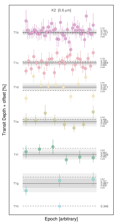
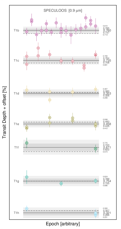
Figure 1: Left: Evolution of the measured transit depths from the global analysis of transit light curves gathered by K2. The horizontal black lines show the medians of the global MCMC posteriors PDFs (with their 1 and 2$\sigma$ confidence intervals, in shades of grey), and dotted lines show the medians of the global MCMC posteriors PDFs for all transits of the same planet observed by Spitzer, as reported in Delrez et al. (2018). Events are ranked in order of capture, left to right (but not linearly in time). Right: Similarly, but for transit observed with SSO. Neither SSO or K2 data show significant variability (less than 3$\sigma$).

3 Results and Discussion

3.1 Temporal evolution of the transit depths

Changes in the transit depths measured for a planet in a given bandpass could result from the evolution of stellar heterogeneities on or outside the chord transited by the planet. Fig. 1 shows the evolution of the transit depths derived from our global analyses of K2 and SSO light curves. These analyses assumed a common transit profile -except for the depths- for each planet and each instrument to better separate the correlated noise from the transit signals and thus guarantee robust results on the transit depths. From those results, we notice that for all planets the depths are consistent from a transit to another, with no discrepancy larger than 3$\sigma$. We computed the standard deviation of the measurements and compare it to the mean value of the measurement errors for each dataset, the values are presented in Table. 3.

Telescope	Planet	# transits	$\sigma$	Mean error
			(%)	(%)
K2	-1b	40	0.084	0.14
	-1c	27	0.080	0.081
	-1d	10	0.11	0.073
	-1e	8	0.077	0.080
	-1f	6	0.072	0.080
	-1g	3	0.087	0.085
	-1h	1	/	/
SPECULOOS	-1b	20	0.069	0.067
	-1c	11	0.080	0.059
	-1d	5	0.057	0.053
	-1e	8	0.055	0.053
	-1f	2	0.055	0.063
	-1g	3	0.044	0.055
	-1h	3	0.044	0.047
Liverpool	-1b	3	0.087	0.081
	-1c	4	0.102	0.062
	-1e	2	0.087	0.081

Table 3: Standard deviation and mean errors of the measured transit depths for all data set. Remark: there are no values for planet h with K2 nor planets d, g, h with the Liverpool telescope because we had only one light curve for each of those planets.

We found that the standard deviation is consistent with the mean of the measurements errors for most of the planets/instruments associations. The exceptions are planet c (SSO, LT) and planet d (K2), where the dispersion of the measurements is actually larger than the mean errors. These mild discrepancies could be genuine, but they could also originate from small-number statistics. Indeed, only 4 transits are used to compute the statistics for LT, 11 transits for SSO for planet c, and 10 transits for planet d.

Looking at the few transits that were observed simultaneously with Spitzer (values from (Delrez et al., 2018)) and K2 (see Table. LABEL:individual_k2) on one hand and with SPECULOOS (see Table. LABEL:individual_spc) and LT (see Table. LABEL:individual_lt) on the other hand, we see that the transit depths values are in agreement with one another (see Table. 4), K2 error bars being significantly larger than Spitzer error bars. For certain transits, the value derived from K2 is larger than the one derived from Spitzer, while for others it is the opposite. We can conclude on the transit observed simultaneously by SPECULOOS and Liverpool as it is unique.

Planet	Epoch	K2	Spitzer
-1b	318	0.830 $\pm$ 0.120	0.751 $\pm$ 0.027
	320	0.669 $\pm$ 0.160	0.699 $\pm$ 0.023
	321	0.988 $\pm$ 0.120	0.801 $\pm$ 0.028
	325	0.866 $\pm$ 0.130	0.732 $\pm$ 0.022
	326	0.693 $\pm$ 0.073	0.724 $\pm$ 0.023
	327	0.851 $\pm$ 0.086	0.663 $\pm$ 0.021
-1c	215	0.604 $\pm$ 0.090	0.672 $\pm$ 0.025
	216	0.686 $\pm$ 0.080	0.652 $\pm$ 0.020
	217	0.797 $\pm$ 0.120	0.735 $\pm$ 0.035
	218	0.809 $\pm$ 0.400	0.674 $\pm$ 0.029
	219	0.663 $\pm$ 0.071	0.668 $\pm$ 0.024
	220	0.830 $\pm$ 0.120	0.725 $\pm$ 0.024
-1d	34	0.304 $\pm$ 0.130	0.384 $\pm$ 0.020
	35	0.412 $\pm$ 0.210	0.382 $\pm$ 0.024
	36	0.361 $\pm$ 0.110	0.348$\pm$ 0.019
-1f	15	0.494 $\pm$ 0.090	0.648 $\pm$ 0.025
-1g	12	0.867 $\pm$ 0.170	0.777 $\pm$ 0.020
Planet	Epoch	SPECULOOS	Liverpool
-1e	53	0.522 $\pm$ 0.055 0.590 $\pm$ 0.057	0.476 $\pm$ 0.069
-1h	17	0.316 $\pm$ 0.057 0.291 $\pm$ 0.044	0.257 $\pm$ 0.035

Table 4: Up: Depth of transits observed simultaneously by K2 and Spitzer. Down: Same but for SPECULOOS and Liverpool telescope.

3.2 Transmission spectra of the TRAPPIST-1 planets

Combining the results of our analyses to the ones presented by Delrez et al. (2018) for Spitzer measurements and by de Wit et al. (2018) for HST/WFC3 measurements, we construct the broadband 0.8-4.5 $\mu$m transit transmission spectra of TRAPPIST-1 planets (Fig. 2).

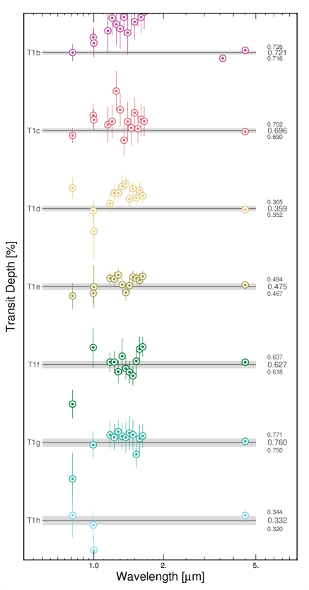
Figure 2: Spectra of the seven TRAPPIST-1 planets. The continuous line is the weighted mean of all non-HST measurements for each planet (with its 1 $\sigma$ confidence, in shades of grey). Each point stands for the median of the global MCMC posterior PDF with error bars at the effective wavelength of the instrument (13 points (14 for T1b) per planet: one for K2, one for SSO, one for LT, 9 for HST/WFC3 and one (two for T1b, 3.6$\mu m$ and 4,5 $\mu m$) for $Spitzer$).

We first note that although the measurements obtained with the HST data do not show features over the WCF3 band (1.1 to 1.7 $\mu$m), the transit depths are significantly deeper than those obtained at other wavelengths for planets b and d. Although this is intriguing, these deeper transits could very well have an instrumental origin. Indeed, as HST is on a low-Earth orbit, it can monitor TRAPPIST-1 for an average of $\sim$50 minutes per orbit out of the $\sim$95 minute orbital duration. The observation of a transit during an HST visit is typically based on 4 or 5 orbits. Due to the small transit durations of the TRAPPIST-1 planets, only one window per visit covers a transit. Yet, although the transit durations of TRAPPIST-1 planets are short, they have roughly the same duration of HST’s observation window leading to a small (and at times negligible) constraint on the baseline level from the in-transit orbit. As HST/WFC3 spectrophotometric observations are affected by orbit-dependent systematic effects, such a limited constraint on the baseline level from the orbit constraining the transit depth can result in a diluted or amplified monochromatic transit depth. The current measurements are particularly limited in such joint “transit depth–baseline level” measurements for planet b (see Fig. 1 of de Wit et al., 2016) and planet d (see Fig. 1 of de Wit et al., 2018)–and reduced for planets c and e–which is consistent with the level of discrepancies seen in Fig. 2. We also note that the transit depth measured for planet f at 0.6$\mu$m (K2) is $\sim$3-$\sigma$ shallower than the mean of the other measurements. This measurement could be explained by its low statistical significance (only 6 transits) or by the detrending of K2 systematic effects and significant stellar variability applied to the light curve before its modeling (see Section 2.1). Nevertheless, there seems to be no significant biases from detrending in the other planets measurements so we would better wait for the analyses of additional transits of planet f in this bandpass to confirm or discard this value. For the other planets, no significant chromatic variation is observed. We note that an argument against a stellar contamination origin of the structure visible in the transit spectra of planets b, d, and f, is the absence of similar structures for planets with similar transit impact parameters, i.e. transiting nearly the same chords of the stellar disk.

Fig. 3 shows the detrended period-folded photometry measured for each planet by K2 and SPECULOOS, as well as the corresponding best-fit transit model. A visual inspection of all individual transit light curves did not reveal such crossing events neither.

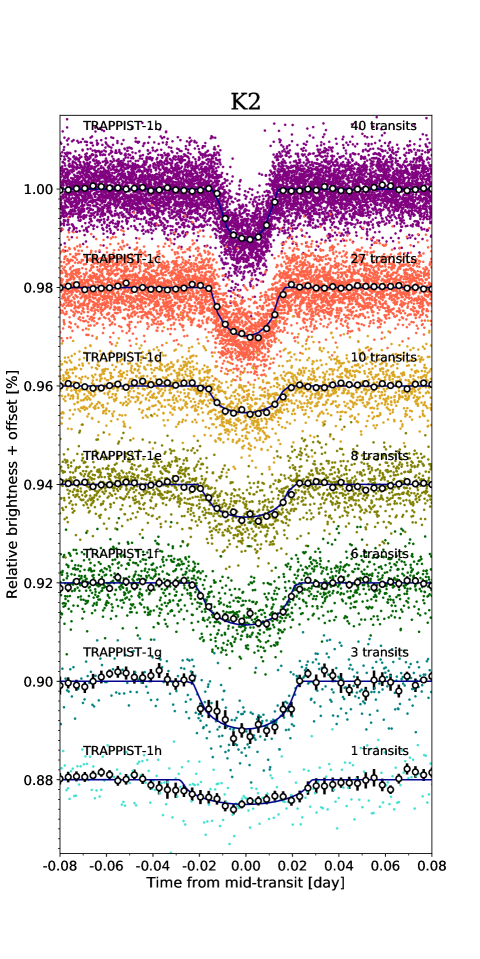
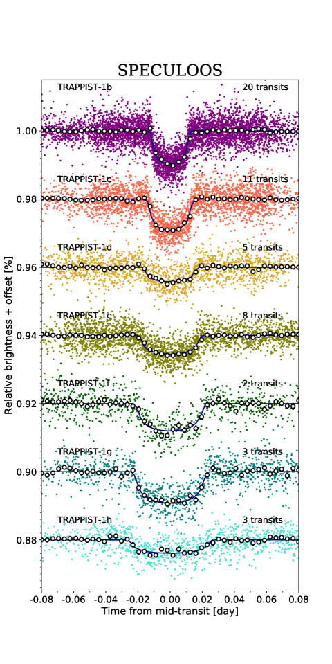
Figure 3: Left: Period-folded photometric measurements obtained by K2 near the transits of the seven planets, corrected for the measured TTVs. Colored dots show the unbinned measurements; open circles depict the 5minute-binned measurements for visual clarity. The best-fit transit models are shown as dark blue lines. The numbers of transits that were observed to produce these combined curves are written on the plot. Right: Similarly but for SSO.

3.3 Confrontation with the stellar contamination model of Z18

The strong stellar contamination inferred for TRAPPIST-1 planets by Z18 is based on the model presented by Rackham et al. (2017), which assumes an heterogeneous photosphere composed of unocculted spots and faculae, and is described by the equation:

$$\epsilon_{\lambda,s+f}=\frac{1}{1-f_{spot}(1-\frac{F_{\lambda,spot}}{F_{\lambda,phot}})-f_{fac}(1-\frac{F_{\lambda,fac}}{F_{\lambda,phot}})},$$ (1)

in which $\epsilon_{\lambda,s+f}$ is the ratio of the observed transit depth $D_{\lambda,obs}$ by the nominal transit depth $D_{\lambda}$ (i.e., the square of the true wavelength-dependent planet-to-star radius ratio) and represents the stellar contamination at wavelength $\lambda$; $F_{\lambda,phot}$, $F_{\lambda,spot}$ and $F_{\lambda,fac}$ refer to the flux of the mean photosphere, spots and faculae respectively; and $f_{spot}$ and $f_{fac}$ refer to the unocculted spot- and faculae- covering fractions (Rackham et al., 2018).

The contamination spectrum $\epsilon_{\lambda,s+f}$ was then multiplied with an assumed wavelength-independent nominal planetary transit depth by Z18 to obtain a transit spectrum whose wavelength-dependence is only due to the stellar contamination. Ultimately, they fitted the percentages of spots and faculae covering fractions, as well as their temperatures and that of the mean photosphere, to represent at best the transit spectra of the TRAPPIST-1 planets that they measured from the HST/WFC3 presented in de Wit et al. (2016) and de Wit et al. (2018). The authors chose to combine spectra of several planets, justifying their choice by the improved signal-to-noise ratio in detecting common spectral features. To enable a straightforward comparison with the Z18 results, we added our measured transit depths of different planets to obtain the same combinations used by Z18.

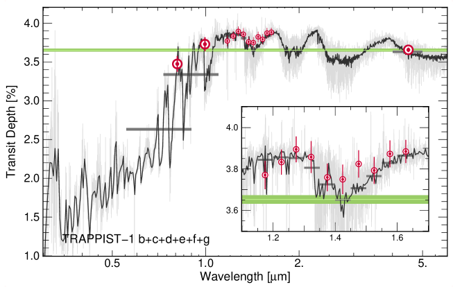
Figure 6: Comparison of the stellar contamination spectrum inferred by Z18 for TRAPPIST-1 b+c+d+e+f+g transits [Zhang et al. (2018)] at two different resolutions (continuous black line and gray line) with the K2 and SSO measurements presented in this work, and the Spitzer and HST/WFC3 presented in Delrez et al. (2018) and de Wit et al. (2016), respectively (red points). The green line represents the weighted mean of all measurements except HST for the reasons outlined earlier in Section. 3.2. Finally, the gray horizontal bars are the band-integrated value for the Z18 model where the integrals are weighted uniformly in wavelength.

The transit depth values obtained from our global analysis of K2, SSO, and LT transits, plus the values measured at 4.5 $\mu$m with Spitzer by Delrez et al. (2018), and at 1.1-1.7 $\mu$m with HST/WFC3 by de Wit et al. (2016) are displayed in Fig.4 for the combination of planets b and c and Fig.6 in Appendix for b+c+d+e+f+g, superimposed with the best-fit stellar contamination model of Z18. Appendix Table 14 gathers the results for those two combination as well as the other combination used in Z18 (d+e+f+g).

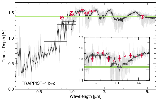
Figure 4: Up: Comparison of the stellar contamination spectrum inferred by Z18 for TRAPPIST-1 b+c transits [Zhang et al. (2018)] at two different resolutions (continuous black line and gray line) with the K2, SSO and LT measurements presented in this work, and the Spitzer and HST/WFC3 presented in Delrez et al. (2018) and de Wit et al. (2016), respectively (red points). The green line represents the weighted mean of all measurements except HST for the reasons outlined earlier in Section. 3.2. Finally, the gray horizontal bars are the band-integrated value for the Z18 model on the effective bandpass of each filter (define as the interval were the product of the filter response and the stellar spectrum is greater than 1%).

The expected transit depths from the best-fit stellar contamination model of Z18, integrated over the spectral bands of the observations, are reported in Appendix Table 14 for the combination of planets b+c, b+c+d+e+f+g, and d+e+f+g, along with the actual measurements. To compute those values, we multiplied the contamination spectrum $\epsilon_{\lambda,s+f}$ inferred in Z18 by the maximum combined transit depth for the corresponding combination of planets $D_{b+c}$, measured from HST/WFC3 data by de Wit et al. (2016).

As shown in Fig. 4 and Table 14, the dramatic drop of the transit depth in the visible predicted by Z18 model is not observed. As a matter of fact, the Z18 prediction for K2 bandpass are discrepant by more than $10\sigma$ from the observations, at $\sim 6.5\sigma$ for SSO, at $\sim 3.5\sigma$ for Liverpool, and $\sim 1.4\sigma$ for Spitzer. The contamination model inferred by Z18 can thus be firmly discarded. It should also be noted that Z18 attributed an inverted water absorption spectral feature to low-significance variations present in their analysis of the HST measurements. However, in de Wit et al. (2016) data we do not see significant traces of this inverted water absorption feature (see zoomed box in Fig. 4).

Finally, in Z18, the sum of the spot and faculae covering fraction approaches 100% with spot of size $R_{spot}=(1.63\pm 0.50)\times 10^{3}km$ (Rackham et al., 2017), while we know from Delrez et al. (2018) that the chords of transit of the TRAPPIST planets cover at least 56% of a stellar hemisphere. Z18’s model should therefore predict a significant number of spot crossing event with amplitudes of the order of 400ppm (Rackham et al., 2017). Quantitatively, according to Z18 for T-1b+T-1c we would expect a frequency rate of 18% spot crossing and 34% of faculae crossing events. We analysed all light curves individually, we see comparable variability in and out of transit, at a significantly lower level than expected (maximum 200ppm) and no asymmetries in the amplitude of the residuals.

While the model of Z18 is discarded by our data, a significant stellar contamination of TRAPPIST-1 planets’ transmission spectra remains a possibility. Indeed, the star’s photosphere is definitely heterogeneous, as its K2 photometry shows a quasi-periodic variability of a couple % with a dominant period of 3.3d that is consistent with the rotation of an evolving inhomogeneous photosphere (Luger et al., 2017), or with the characteristic timescale between flares followed by spot brightening (Morris et al., 2018, hereafter M18). The photometry of the TRAPPIST telescope (Gillon et al., 2011) also shows variability of similar amplitude, with a dominant period identified to be $\sim$1.4d by Gillon et al. (2016). We note that this latter value is close to the alias of 3.3d, suggesting that the periodogram analysis done by Gillon et al. (2016) did not identify the right period because of the discontinuous sampling of the TRAPPIST observations, or that the variability is only quasi-periodic.

3.4 On the possible photospheric structure of TRAPPIST-1

3.4.1 Giant cold spots?

While not stated explicitly, the photospheric model of Z18 considered solar-like spots + faculae, and not giant spots + faculae, as this is the only way for the percentages obtained for the best fit ($\sim 30\%$ of spots and $\sim 63\%$ of faculae) to agree to a certain extent with the predictions of R18 on which it is based ($8_{-7}^{+18}\%$ of spots and $54_{-46}^{+16}\%$ of faculae). At this point, it is worth explaining what is meant by giant spots and solar spots. The “solar spot” model used in R18 relies on small time-steady rotating spots to produce the predicted variability amplitude in transit depth. As the variations in flux cancel out when the spots rotate onto and off of the visible photosphere, a large number of spots are required to reach the predicted transit depth variation, leading to a large, heterogeneous, but nearly time-steady component. Conversely, the “giant spot” model shows large amplitude variability with small covering fraction as there is no cancellation between spots rotating on and off, and giant spots therefore have a variable component.

If instead of considering solar-type spots + faculae, we consider giants spots + faculae, we notice that the prediction from CPAT (composite photosphere and atmospheric transmission) model of Rackham et al. (2017) on the transit depth variations are much less pessimistic (not more than 0.7% difference between transit depth at $4.5\mu m$ and at $0.6\mu m$ for an M9V type star, R18, Fig. 7). We could thus imagine that the photosphere of TRAPPIST-1 is more likely to host giant spots than solar-like spots. In this case it is worth noticing that according to the predictions of R18, for Earth-twin type planets, the stellar heterogeneity does not jeopardize the detection of planetary atmospheric features with JWST anymore. Considering a precision of 30ppm with JWST, R18 indicates that for a M8V type star like TRAPPIST-1 the depth variations due to atmospheric features should be of the order of 90ppm whereas the variations due to stellar heterogeneity should be of the order of $\approx$17ppm, consequently allowing detections of planetary features despite stellar contamination.

As discussed above, the TRAPPIST-1 planets cover a significant part of the hemisphere of the star from latitudes up to $30^{\circ}$, latitudes where we find spots on the Sun (Miletskii and Ivanov, 2009). The next logical step is to look for giant spot-crossing events in the transits of the TRAPPIST-1 planets. In the observations carried out by Spitzer the in and out of transit variability was more likely attributed to systematic effects or granulation variability (see Delrez et al., 2018). Yet the spot-to-photosphere contrast is wavelength-dependent such that spot-crossing events are not detectable at all wavelengths (see Ballerini et al., 2012). However, our analyses of observations in the visible and near-IR carried out by K2, SPECULOOS and Liverpool telescope do not show transit depth variability that could have been attributed to stellar spot crossings during transits (see Section. 3.1). A possible scenario allows for giant spots consists of high-latitude spots that never cross the planets’ transit chords, in a similar manner as the circumpolar spots observed for young mid- to late-type M-dwarfs not older than 1 Gyr (see Barnes et al., 2015); this potentially could explain the variability detected in the K2 bandpass. However, TRAPPIST-1 is not a young dwarf, its age having been estimated to be 7.6 $\pm$ 2.2 Gyr by Burgasser and Mamajek (2017), and the out-of-transit rotational variability resulting from a giant, dark polar spot does not match the small observed variability of 2ppm (Delrez et al., 2018) seen in the infrared (Morris et al., 2018). In addition, the giant spot model is disfavored by the correlations between flares and spot brightening seen in the K2 dataset, which indicates that the brightening is not due to spots rotating out of view, but rather due to a temporary brightening of the star which follows each flare event (Morris et al., 2018).

3.4.2 Small hot faculae?

In their studies, R18 and Z18 assumed that the active regions of TRAPPIST-1 are qualitatively similar to solar active regions in the spot and facular flux contrasts, and in the relative areas of each component. However, there is abundant evidence that the Sun is a poor analog for the starspot distributions of fully-convective stars (Donati et al., 2003; Morin et al., 2008, 2010; Barnes et al., 2015), which are likely driven by a different magnetic dynamo process (Donati, 2011; Reiners, 2012).

Morris et al. (2018) presented an alternative, empirically-driven hypothetical spot distribution for TRAPPIST-1, consisting of a few small, bright (hot) spots. The proposed hot spots, which are correlated with the brightest flares, drive the modulation with an 3.3 day period in the K2 bandpass without generating a corresponding signal in the Spitzer 4.5 $\mu$m band, in agreement with the observations.

We predict the effect of the hot spots of Morris et al. (2018) at 4500 K on the transit depths of TRAPPIST-1 b and c in Fig. 5. These spots produce a nearly-flat contamination spectrum for wavelengths $\gtrsim 0.7\mu$m, and modest flux dilution (shallower transit depths) in the K2 bandpass. We find that spots with temperatures up to 4500 K are consistent at $\sim 2\sigma$ with the observed transit depths, excluding the HST data for the reasons discussed above.

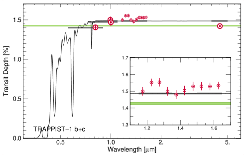
Figure 5: Comparison of the observed transit depth variation (red points) with the predictions from stellar contamination due to the bright spots proposed by Morris et al. (2018) for spots at 4500K (gray continuous line). We used PHOENIX model atmospheres with photospheric temperature 2511 K and the hot spot properties in M18.

4 Conclusion

We performed individual and global analyses of 169 transit light curves obtained from space with K2 and from the ground with SSO and LT as well as the light curves obtained from mid-IR observations with Spitzer and near-IR with HST/WFC3 to construct the broadband transmission spectra of the TRAPPIST-1 planets over the 0.8-4.5$\mu m$ spectral range. While we could not find any significant temporal variability of the transit depths measured by the same instrument, our analysis reveals chromatic structures at the level of only 200-300ppm in the transit transmission spectra of planets b, d, and f. These results enable us to discard the highly heterogeneous photospheric model presented by Z18 and their subsequent conclusions regarding the potential of JWST to characterize the atmospheric properties of TRAPPIST-1 planets by transit transmission spectroscopy. We identify two possible photospheric structures for TRAPPIST-1 that could agree with our results, one dominated by a few high-latitude giant (cold) spots, which is disfavored for different reasons, and the other by a few small and hot ($>$ 4000K) faculae. Although our measurements do not confirm the conclusions of Z18, they cannot rule out a significant stellar contamination of the planets’ transmission spectra. The recent announcement of the delayed launch of JWST gives us the opportunity to investigate further the photospheric structure of TRAPPIST-1 -notably through photometric monitoring at different wavelengths- and its impact on the planets’ transmission spectra. Furthermore, the JWST delay offers more time for the development of new strategies to optimally disentangle the stellar (contamination) and planetary (transmission) effects.

5 Acknowledgement

We thank Jon Marchant and Chris Copperwheat for their kind and frequent help in scheduling the Liverpool Telescope. The Liverpool Telescope is operated on the island of La Palma by Liverpool John Moores University in the Spanish Observatorio del Roque de los Muchachos of the Instituto de Astrofisica de Canarias with financial support from the UK Science and Technology Facilities Council.

The research leading to these results has received funding from the European Research Council (ERC) under the FP/2007-2013 ERC grant agreement no. 336480, and under the H2020 ERC grant agreement no. 679030; and from an Actions de Recherche Concertée (ARC) grant, financed by the Wallonia-Brussels Federation. This work was also partially supported by a grant from the Simons Foundation (PI Queloz, grant number 327127), as well as by the MERAC foundation (PI Triaud). LD acknowledges support from the Gruber Foundation Fellowship. VVG and MG are F.R.S.-FNRS Research Associates. JdW is grateful for the financial support received for the SPECULOOS Project from the Heising-Simons Foundation, P. Gilman, and C. & L. Masson. EJ is F.R.S.-FNRS. EA acknowledges USA NSF grant 1615315, the Guggenheim Foundation, and NASA Virtual Planetary Laboratory. Senior Research Associate. B-OD acknowledges support from the Swiss National Science Foundation in the form of a SNSF Professorship (PP00P2_163967). AJB acknowledges funding support from the US-UK Fulbright Scholarship programme.

Appendix A Description of the data

Table 5: Description of transit light curves measured for TRAPPIST-1 planets by SPECULOOS-South.

Planet	Date	Telescope	Number of points	Epoch	Baseline	$\beta_{w}$	$\beta_{r}$	CF
b	18 Jun. 2017	Europa	487	398	$p(fwhm^{1})$	1.22	1.20	1.47
	30 Jun. 2017	Io	196	406	$p(t^{1})$	1.04	1.00	1.04
	30 Jun. 2017	Europa	242	406	$p(t^{1})+p(xy^{1})$	1.02	1.89	1.93
	01 Aug. 2017	Europa	273	427	$p(fwhm^{1})$	1.28	1.09	1.40
	07 Aug. 2017	Europa	228	431	$p(fwhm^{1})$	1.07	1.49	1.59
	13 Aug. 2017	Europa	263	435	$p(t^{1})$	1.18	1.18	1.39
	13 Aug. 2017	Io	434	435	$p(t^{1})$	1.04	1.15	1.19
	19 Aug. 2017	Europa	287	439	$p(s)$	1.09	1.24	1.35
	25 Aug. 2017	Europa	284	443	$p(s)$	1.35	1.3	1.75
	20 Sep. 2017	Europa	254	460	$p(t^{1})+p(xy^{1})$	1.29	1.04	1.33
	23 Sep. 2017	Io	264	462	$p(xy^{1})$	0.99	1.30	1.30
	08 Oct. 2017	Europa	257	472	$p(xy^{1})$	1.3	1.3	1.69
	20 Oct. 2017	Europa	227	480	$p(t^{1})$	1.06	1.2	1.28
	30 Nov. 2017	Europa	260	507	$p(s)$	1.22	1.21	1.48
	30 Nov. 2017	Io	267	507	$p(t^{1})+p(fwhm^{1})$	1.21	1.00	1.21
	03 Dec. 2017	Io	262	509	$p(t^{1})$	1.13	1.37	1.55
	03 Dec. 2017	Europa	259	509	$p(t^{1})$	1.04	1.00	1.04
	06 Dec. 2017	Europa	212	511	$p(t^{1})$	1.89	1.00	1.89
	28 Aug. 2017	Europa	154	445	$p(s)$	1.13	1.07	1.21
	28 Aug. 2017	Io	156	445	$p(s)$	1.16	1.00	1.16
c	28 Aug. 2017	Europa	178	294	$p(fwhm^{1})$	1.14	1.00	1.14
	28 Aug. 2017	Io	272	294	$p(t^{1})$	1.10	1.61	1.76
	14 Sep. 2017	Europa	247	301	$p(t^{1})$	1.08	1.35	1.45
	15 Sep. 2017	Io	339	301	$p(t^{1})+p(a^{1})p(fwhm^{1})$	1.95	1.00	1.95
	06 Oct. 2017	Europa	364	310	$p(t^{2})$	1.12	1.19	1.33
	18 Oct. 2017	Europa	264	315	$p(t^{1})$	1.13	1.04	1.18
	21 Nov. 2017	Europa	318	329	$p(b^{1})$	1.14	1.21	1.37
	21 Nov. 2017	Io	265	329	$p(t^{1})+p(fwhm^{1})$	1.07	1.37	1.47
	08 Dec. 2017	Europa	240	336	$p(s)$	1.11	1.18	1.31
	08 Dec. 2017	Io	243	336	$p(a^{1})$	1.08	1.27	1.38
	04 Nov. 2017	Europa	267	322	$p(t^{1})$	1.19	1.00	1.19
d	26 Jul. 2017	Europa	422	72	$p(s)$	1.03	1.78	1.82
	03 Aug. 2017	Europa	325	74	$p(t^{1})$	1.18	1.31	1.55
	03 Aug. 2017	Io	378	74	$p(t^{1})+p(fwhm^{1})$	1.16	1.38	1.59
	07 Aug. 2017	Europa	320	75	$p(t^{1})+p(fwhm^{1})$	1.17	1.00	1.17
	07 Oct. 2017	Europa	322	90	$p(t^{1})+p(xy^{1})$	1.07	1.13	1.21
e	29 Jun. 2017	Europa	422	45	$p(s)$	1.19	1.00	1.19
	29 Jun. 2017	Io	401	45	$p(t^{1})$	1.06	1.33	1.41
	05 Jul. 2017	Europa	448	46	$p(a^{1})+p(fwhm^{1})$	1.44	1.10	1.58
	05 Jul. 2017	Io	445	46	$p(t^{2})+p(fwhm^{1})$	1.13	1.00	1.13
	17 Aug. 2017	Europa	388	53	$p(s)$	0.93	1.39	1.30
	17 Aug. 2017	Io	198	53	$p(s)$	0.91	1.05	0.95
	23 Aug. 2017	Europa	418	54	$p(s)$	1.14	1.82	2.08
	23 Aug. 2017	Io	415	54	$p(s)$	1.14	1.35	1.53
f	27 Aug. 2017	Europa	363	35	$p(s)$	1.14	1.55	1.76
	10 Oct. 2017	Europa	608	40	$p(s)$	1.11	1.42	1.58
g	19 Jun. 2017	Europa	497	21	$p(fwhm^{1})$	0.95	1.05	1.00
	26 Jul. 2017	Europa	475	22	$p(s)$	1.24	1.48	1.83
	27 Jul. 2017	Europa	533	23	$p(s)$	1.23	1.08	1.34
h	27 Jul. 2017	Europa	741	16	$p(a^{1})$	1.28	1.70	2.18
	15 Aug. 2017	Io	412	17	$p(t^{1})$	1.01	1.08	1.19
	15 Aug. 2017	Europa	434	17	$p(a^{1})$	0.97	1.81	1.77

• Notes. For each light curve, this table shows the date of acquisition, the used instrument, the number of data points, the epoch based on the transit ephemeris presented in (Delrez et al., 2018), the selected baseline function (see Section.2) and the deduced values for $\beta_{w}$ , $\beta_{r}$ , and $CF=\beta_{r}*\beta_{w}$ (see Section.2). For the baseline function, p($\epsilon^{N}$ ) denotes, respectively, a N-order polynomial function of time ($\epsilon$ = t), the full width at half maximum ($\epsilon$ = fwhm), x and y positions ($\epsilon$ = xy), the background ($\epsilon$ = b), the airmass ($\epsilon$ = a) and a scalar ($\epsilon$ = s).

Table 6: Same as Table LABEL:baseline_spc, but for K2.

Planet	Date	Number of points	Epoch	Baseline	$\beta_{w}$	$\beta_{r}$	CF
b	18 Dec. 2016	301	277	$p(t^{2})$	0.86	1.84	1.59
	20 Dec. 2016	303	278	$p(t^{3})$	0.88	1.68	1.47
	21 Dec. 2016	303	279	$p(t^{1})$	0.82	1.08	0.95
	23 Dec. 2016	304	280	$p(t^{1})$	0.84	1.00	0.84
	26 Dec. 2016	242	282	$p(s)$	0.91	1.11	1.01
	27 Dec. 2016	241	283	$p(s)$	0.92	1.08	1.00
	29 Dec. 2016	305	284	$p(t^{2})$	0.91	1.38	1.26
	30 Dec. 2016	304	285	$p(s)$	0.84	1.34	1.13
	01 Jan. 2017	303	286	$p(t^{2})$	0.86	1.01	0.87
	02 Jan. 2017	305	287	$p(t^{1})$	0.90	1.74	1.57
	04 Jan. 2017	303	288	$p(s)$	0.80	1.74	1.40
	05 Jan. 2017	214	289	$p(t^{1})$	0.81	1.00	1.81
	07 Jan. 2017	302	290	$p(t^{3})$	0.87	1.15	1.01
	08 Jan. 2017	269	291	$p(t^{3})$	0.93	1.09	1.02
	10 Jan. 2017	303	292	$p(s)$	0.87	1.82	1.57
	11 Jan. 2017	303	293	$p(t^{3})$	0.84	1.07	0.91
	13 Jan. 2017	305	294	$p(t^{1})$	0.89	1.12	1.00
	14 Jan. 2017	305	295	$p(t^{2})$	0.90	1.28	1.16
	16 Jan. 2017	297	296	$p(s)$	0.91	1.63	1.49
	17 Jan. 2017	215	297	$p(t^{1})$	0.84	1.53	1.28
	19 Jan. 2017	206	298	$p(s)$	0.82	1.68	1.39
	20 Jan. 2017	259	299	$p(s)$	0.92	1.22	1.13
	22 Jan. 2017	304	300	$p(t^{1})$	0.88	1.48	1.32
	23 Jan. 2017	303	301	$p(t^{4})$	0.89	1.00	0.89
	25 Jan. 2017	302	302	$p(s)$	0.82	1.19	0.87
	26 Jan. 2017	302	303	$p(t^{1})$	0.86	1.43	1.23
	29 Jan. 2017	293	305	$p(t^{2})$	0.87	1.04	0.91
	31 Jan. 2017	304	306	$p(t^{3})$	0.90	1.22	1.11
	07 Feb. 2017	306	311	$p(t^{3})$	0.81	1.09	0.87
	10 Feb. 2017	300	313	$p(s)$	0.97	1.63	1.58
	12 Feb. 2017	304	314	$p(s)$	1.04	1.31	1.36
	13 Feb. 2017	302	315	$p(t^{4})$	0.92	1.12	1.03
	15 Feb. 2017	304	316	$p(t^{2})$	0.94	1.34	1.26
	16 Feb. 2017	303	317	$p(t^{3})$	0.94	1.16	1.09
	18 Feb. 2017	296	318	$p(t^{1})$	0.81	1.09	0.87
	19 Feb. 2017	305	319	$p(t^{1})$	0.88	1.11	0.98
	21 Feb. 2017	206	320	$p(s)$	0.91	1.54	1.40
	24 Feb. 2017	294	322	$p(t^{1})$	0.95	1.08	1.02
	26 Feb. 2017	305	323	$p(t^{3})$	0.87	1.00	0.87
	01 Mar. 2017	196	325	$p(s)$	0.95	1.19	1.13
	01 Mar. 2017	291	326	$p(t^{1})$	0.93	1.00	0.93
	04 Mar. 2017	305	327	$p(s)$	1.02	1.89	1.93
c	18 Dec. 2016	304	189	$p(t^{1})$	0.83	1.00	0.83
	20 Dec. 2016	219	190	$p(t^{2})$	0.87	1.28	1.07
	22 Dec. 2016	217	191	$p(s)$	0.81	1.73	1.41
	25 Dec. 2016	304	192	$p(s)$	0.86	1.64	1.41
	27 Dec. 2016	238	193	$p(s)$	0.83	1.00	0.83
	30 Dec. 2016	303	194	$p(t^{1})$	0.80	1.30	1.04
	03 Jan. 2017	232	196	$p(s)$	0.89	2.14	1.90
	05 Jan. 2017	185	197	$p(t^{1})$	0.89	1.06	0.94
	07 Jan. 2017	250	198	$p(t^{4})$	0.88	1.22	1.08
	11 Jan. 2017	304	199	$p(s)$	0.85	1.51	1.28
	13 Jan. 2017	302	200	$p(s)$	0.84	1.35	1.14
	16 Jan. 2017	249	201	$p(t^{2})$	0.81	1.25	1.03
	18 Jan. 2017	244	202	$p(s)$	0.80	1.09	0.87
	20 Jan. 2017	284	203	$p(t^{1})$	0.84	1.17	0.98
	23 Jan. 2017	305	204	$p(t^{3})$	0.86	1.00	0.86
	25 Jan. 2017	304	205	$p(s)$	0.91	1.46	1.34
	27 Jan. 2017	233	206	$p(s)$	0.84	1.29	1.08
	30 Jan. 2017	216	207	$p(t^{1})$	0.91	1.13	1.03
	06 Feb. 2017	188	210	$p(t^{3})$	0.85	1.00	0.85
	09 Feb. 2017	221	211	$p(t^{1})$	0.87	1.31	1.14
	11 Feb. 2017	303	212	$p(t^{2})$	0.88	1.18	1.05
	14 Feb. 2017	304	213	$p(t^{3})$	0.85	1.77	1.51
	16 Feb. 2017	258	214	$p(t^{2})$	0.95	1.69	1.60
	18 Feb. 2017	253	215	$p(t^{3})$	0.85	1.11	1.94
	21 Feb. 2017	210	216	$p(t^{1})$	0.92	1.42	1.31
	23 Feb. 2017	307	217	$p(t^{2})$	0.89	1.31	1.17
	26 Feb. 2017	304	218	$p(s)$	0.89	2.00	1.79
	28 Feb. 2017	306	219	$p(t^{2})$	0.93	1.00	0.93
	03 Mar. 2017	305	220	$p(t^{3})$	0.87	1.00	0.87
d	16 Dec. 2016	305	44	$p(s)$	0.84	1.13	0.96
	20 Dec. 2016	203	45	$p(t^{4})$	0.79	1.00	0.79
	28 Dec. 2016	304	47	$p(t^{4})$	0.88	1.13	1.00
	01 Jan. 2017	186	48	$p(t^{1})$	0.83	1.00	0.83
	05 Jan. 2017	198	49	$p(s)$	0.89	1.01	0.90
	09 Jan. 2017	305	50	$p(t^{3})$	0.79	1.00	0.79
	13 Jan. 2017	304	51	$p(t^{1})$	0.84	1.09	0.91
	17 Jan. 2017	491	52	$p(s)$	0.91	1.48	1.35
	21 Jan. 2017	306	53	$p(t^{1})$	0.87	1.30	1.13
	25 Jan. 2017	298	54	$p(t^{3})$	0.87	1.45	1.27
	07 Feb. 2017	210	57	$p(s)$	0.87	1.00	0.87
	23 Feb. 2017	305	61	$p(t^{1})$	0.87	1.11	0.97
	27 Feb. 2017	304	61	$p(t^{1})$	0.93	1.40	1.30
	03 Mar. 2017	306	63	$p(s)$	0.97	1.00	0.97
e	17 Dec. 2016	259	70	$p(t^{1})$	0.84	1.40	1.17
	23 Dec. 2016	303	71	$p(t^{1})$	0.87	1.27	1.11
	04 Jan. 2016	296	73	$p(t^{1})$	0.88	2.01	1.78
	10 Jan. 2016	251	74	$p(t^{1})$	0.89	1.20	1.08
	16 Jan. 2016	306	75	$p(t^{1})$	0.87	1.04	0.90
	22 Jan. 2016	304	76	$p(t^{2})$	0.83	1.05	0.89
	28 Jan. 2016	304	77	$p(t^{1})$	0.91	1.00	0.91
	10 Feb. 2016	304	79	$p(t^{1})$	0.90	1.55	1.40
f	22 Dec. 2016	260	8	$p(s)$	0.90	1.52	1.37
	31 Dec. 2016	304	9	$p(s)$	0.88	1.16	1.03
	09 Jan. 2017	304	10	$p(s)$	0.90	1.79	1.62
	19 Jan. 2017	223	11	$p(t^{1})$	0.89	1.15	1.03
	15 Feb. 2017	303	14	$p(s)$	0.87	1.67	1.46
	15 Feb. 2017	301	15	$p(s)$	0.89	1.30	1.15
g	10 Jan. 2017	199	8	$p(s)$	0.89	1.05	0.93
	16 Feb. 2017	256	11	$p(t^{1})$	0.88	1.51	1.34
	01 Mar. 2017	156	12	$p(s)$	0.96	1.41	1.35
h	02 Jan. 2017	304	5	$p(t^{1})$	0.82	1.06	0.88

Table 7: Same as Table LABEL:baseline_spc, but for LT.

Planet	Date	Number of points	Epoch	Baseline	$\beta_{w}$	$\beta_{r}$	CF
b	31 May. 2017	139	386	$p(t^{1})+p(fwhm^{1})$	1.23	1.00	1.23
	23 Jul. 2017	152	421	$p(s)$	1.00	1.09	1.09
	29 Jul. 2017	153	425	$p(s)$	0.99	1.08	1.07
	5 Aug. 2017	156	429	$p(t^{1})$	1.58	1.00	1.58
c	01 Jul. 2017	157	270	$p(s)$	0.88	1.43	1.26
	07 Sep. 2017	178	298	$p(t^{1}))$	0.95	1.00	0.95
	19 Sep. 2017	178	303	$p(t^{1})$	1.31	1.24	1.63
	28 Oct. 2017	176	319	$p(s)$	1.11	1.31	1.46
	5 Aug. 2017	187	284	$p(s)$	1.51	1.25	1.79
d	21 Sep. 2017	227	113	$p(t^{1})+p(fwhm^{1})$	1.45	1.05	1.52
e	17 Aug. 2017	274	110	$p(t^{1})$	1.30	1.28	1.66
	17 Aug. 2017	202	118	$p(s)$	1.00	1.55	1.55
h	15 Aug. 2017	378	17	$p(t^{1})$	1.00	1.00	1.00

Appendix B Results from the individual analysis

Table 8: Transit timings and depths obtained from the individual analyses of SPECULOOS light curves. Each row represents a transit, the first column gives the planet’s name, the second the epoch of the transit, the third the mid-transit timing and the corresponding error resulting from the analysis and the last column the transit depth and corresponding error resulting from the analysis.

Planet	Epoch	Transit timing [$BJD_{TDB}-2450000$]		Transit depth (%)
b	398	7923.84586	0.00043	0.764	0.060
	406	7935.93284	0.00028	0.842	0.047
	406	7935.93316	0.00053	0.893	0.088
	427	7967.66254	0.00053	0.686	0.068
	431	7973.70588	0.00058	0.759	0.078
	435	7979.74899	0.00030	0.835	0.058
	435	7979.74864	0.00034	0.738	0.048
	439	7985.79209	0.00034	0.721	0.052
	443	7991.83579	0.00041	0.845	0.079
	460	8017.52106	0.00041	0.774	0.079
	462	8020.54219	0.00036	0.758	0.056
	472	8035.65192	0.00065	0.801	0.085
	480	8047.73788	0.00059	0.676	0.094
	507	8088.53228	0.00033	0.796	0.060
	507	8088.53206	0.00026	0.920	0.059
	509	8091.55411	0.00036	0.878	0.065
	509	8091.55364	0.00035	0.809	0.045
	511	8094.57595	0.00067	0.822	0.120
	445	7994.85842	0.00047	0.819	0.084
	445	7994.85833	0.00051	0.855	0.083
c	294	7994.81758	0.0004	0.835	0.068
	294	7994.81885	0.00065	0.695	0.082
	301	8011.77150	0.00046	0.826	0.066
	301	8011.77102	0.00036	0.878	0.078
	310	8033.56743	0.00041	0.801	0.060
	315	8045.67598	0.00035	0.738	0.055
	329	8079.58077	0.00042	0.649	0.055
	329	8079.58172	0.00050	0.679	0.055
	336	8096.53342	0.00037	0.789	0.055
	336	8096.53330	0.00051	0.819	0.062
	322	8062.62794	0.00039	0.727	0.160
d	72	7961.73755	0.00012	0.394	0.057
	74	7969.83771	0.00020	0.264	0.062
	74	7969.83665	0.00100	0.375	0.065
	75	7973.88834	0.00140	0.401	0.062
	90	8034.62829	0.00063	0.405	0.048
e	45	7934.83251	0.00088	0.442	0.046
	45	7934.82990	0.00092	0.417	0.044
	46	7940.93132	0.00049	0.547	0.048
	46	7940.92923	0.00061	0.454	0.055
	53	7983.62886	0.00095	0.522	0.055
	53	7983.62706	0.00053	0.590	0.057
	54	7989.73173	0.00210	0.449	0.065
	54	7989.72916	0.00067	0.458	0.045
f	35	7993.63410	0.00070	0.741	0.074
	40	8039.66021	0.00084	0.639	0.056
g	21	7924.76924	0.00055	0.791	0.051
	24	7961.82599	0.00075	0.723	0.059
	29	7813.60697	0.00200	0.867	0.17
h	16	7962.86330	0.0018	0.372	0.052
	17	7981.63159	0.0016	0.290	0.046
	17	7981.63059	0.0030	0.301	0.046

Table 9: Transit timings and depths obtained from the individual analyses of K2 light curves. Each row represents a transit, the first column gives the planet’s name, the second the epoch of the transit, the third the mid-transit timing and the corresponding error resulting from the analysis and the last column the transit depth and corresponding error resulting from the analysis.

Planet	Epoch	Transit timing [$BJD_{TDB}-2450000$]		Transit depth (%)
b	277	7741.02841	0.0011	0.959	0.200
	278	7742.54031	0.00120	0.804	0.160
	279	7744.05191	0.00063	0.740	0.095
	280	7745.56254	0.00071	0.721	0.080
	282	7748.58511	0.00071	0.728	0.084
	283	7750.09533	0.00150	0.776	0.110
	284	7751.60539	0.00093	0.799	0.150
	285	7753.11716	0.00064	0.746	0.100
	286	7754.62846	0.00071	0.720	0.089
	287	7756.13952	0.00110	0.775	0.150
	288	7757.64925	0.00098	0.784	0.100
	289	7759.16120	0.00100	0.689	0.080
	290	7760.67229	0.00086	0.743	0.097
	291	7762.18295	0.00090	0.569	0.055
	292	7763.69272	0.00110	0.741	0.130
	293	7765.20352	0.00056	0.843	0.083
	294	7766.71525	0.00074	0.766	0.089
	295	7768.22451	0.00089	0.932	0.180
	296	7769.73779	0.00140	0.666	0.200
	297	7771.24857	0.00140	0.673	0.150
	298	7772.75851	0.00120	0.643	0.120
	299	7774.26913	0.00085	0.889	0.110
	300	7775.78022	0.00099	0.736	0.120
	301	7777.28984	0.00069	0.685	0.085
	302	7778.80191	0.00084	0.632	0.070
	303	7780.31394	0.00058	0.719	0.089
	305	7783.33438	0.00110	0.604	0.082
	306	7784.84448	0.00150	0.555	0.110
	311	7792.40048	0.00110	0.788	0.092
	313	7795.42062	0.00110	0.902	0.210
	314	7796.93214	0.00093	0.772	0.130
	315	7798.44260	0.00065	0.836	0.120
	316	7799.95368	0.00100	0.822	0.200
	317	7801.46362	0.00099	0.707	0.100
	318	7802.97696	0.00099	0.830	0.280
	319	7804.48723	0.00065	0.783	0.099
	320	7805.99725	0.00110	0.669	0.160
	322	7809.02001	0.00063	0.988	0.120
	323	7810.52858	0.00059	0.809	0.120
	325	7813.55299	0.00079	0.866	0.130
	326	7815.06305	0.00067	0.693	0.073
	327	7816.57407	0.00058	0.851	0.086
c	189	7740.53417	0.00083	0.589	0.091
	190	7742.95370	0.00100	0.737	0.091
	191	7745.37836	0.00200	0.656	0.150
	192	7747.79745	0.00100	0.864	0.150
	193	7750.21906	0.00092	0.699	0.065
	194	7752.64173	0.00100	0.652	0.079
	196	7757.48363	0.00150	0.770	0.160
	197	7759.90355	0.00081	0.552	0.077
	198	7762.32917	0.00098	0.697	0.100
	199	7764.74926	0.00120	0.818	0.120
	200	7767.17041	0.00120	0.791	0.160
	201	7769.59305	0.00082	0.579	0.090
	202	7772.01577	0.00110	0.846	0.081
	203	7774.43531	0.00084	0.732	0.090
	204	7776.85884	0.00084	0.789	0.130
	205	7779.27985	0.00150	0.713	0.110
	206	7781.70135	0.00081	0.785	0.081
	207	7784.12337	0.00080	0.837	0.100
	210	7791.38904	0.00080	0.588	0.086
	211	7793.81167	0.00085	0.674	0.082
	212	7796.23257	0.00072	0.771	0.085
	213	7798.65449	0.00110	0.798	0.140
	214	7801.07700	0.00084	0.771	0.140
	215	7803.49803	0.00100	0.604	0.090
	216	7805.91971	0.00068	0.686	0.080
	217	7808.34120	0.00120	0.797	0.120
	218	7810.76238	0.00210	0.809	0.400
	219	7813.18452	0.00110	0.663	0.071
	220	7815.60631	0.00070	0.856	0.074
d	17	7738.99254	0.00400	0.286	0.110
	18	7743.03818	0.00120	0.564	0.092
	20	7751.14013	0.00180	0.468	0.100
	21	7755.18855	0.00140	0.537	0.120
	22	7759.24739	0.00180	0.461	0.073
	23	7763.28944	0.00130	0.419	0.062
	24	7767.34079	0.00330	0.318	0.130
	25	7771.39074	0.00420	0.453	0.120
	26	7775.44035	0.00180	0.466	0.090
	27	7779.48982	0.00320	0.603	0.240
	30	7791.64154	0.00098	0.570	0.076
	34	7807.84073	0.00570	0.304	0.130
	35	7811.88917	0.00460	0.412	0.210
	36	7815.94153	0.00170	0.361	0.110
e	13	7739.67183	0.00160	0.509	0.100
	14	7745.77293	0.00180	0.514	0.110
	16	7757.96796	0.00310	0.587	0.110
	17	7764.07021	0.00150	0.521	0.120
	18	7770.17149	0.00240	0.447	0.130
	19	7776.26457	0.00190	0.383	0.075
	20	7782.36274	0.00190	0.430	0.070
	22	7794.56245	0.00180	0.599	0.089
f	8	7745.03067	0.00210	0.613	0.160
	9	7754.23474	0.00140	0.653	0.110
	10	7763.44545	0.00240	0.651	0.130
	11	7772.64854	0.00180	0.461	0.061
	14	7800.27394	0.00220	0.524	0.120
	15	7809.47737	0.00270	0.494	0.090
g	8	7764.19229	0.00180	0.559	0.071
	11	7801.25085	0.00120	0.727	0.100
	12	7813.60698	0.00200	0.867	0.170
h	5	7756.38806	0.00300	0.346	0.058

Table 10: Transit timings and depths obtained from the individual analyses of LT light curves. Each row represents a transit, the first column gives the planet’s name, the second the epoch of the transit, the third the mid-transit timing and the corresponding error resulting from the analysis and the last column the transit depth and corresponding error resulting from the analysis.

Planet	Epoch	Transit timing [$BJD_{TDB}-2450000$]		Transit depth (%)
b	386	7905.71514	0.00088	0.848	0.130
	421	7958.59599	0.00038	0.696	0.062
	425	7964.63878	0.00043	0.830	0.063
	429	7970.68530	0.00051	0.706	0.063
c	270	7936.69651	0.00040	0.721	0.053
	298	8004.50488	0.00052	0.879	0.058
	303	8016.61384	0.00087	0.612	0.090
	319	8055.36295	0.00044	0.765	0.059
	284	7970.60046	0.00085	0.638	0.070
d	86	8018.43071	0.00096	0.353	0.027
e	53	7983.62882	0.00140	0.481	0.075
	56	8032.43398	0.00180	0.475	0.100
h	17	7981.63343	0.00110	0.257	0.035

Appendix C Results from the global analysis

Table 11: Median values and 1-$\sigma$ limits of the posterior PDFs deduced for the timings and depths from their global analyses for SPECULOOS observations. Each row represents a transit, the first column gives the planet’s name, the second the epoch of the transit, the third the mid-transit timing and the corresponding error resulting from the analysis and the last column the transit depth and corresponding error resulting from the analysis.

Planet	Epoch	Transit timing [$BJD_{TDB}-2450000$]		Transit depth (%)
b	398	7923.84588	0.00043	0.744	0.053
	406	7935.93286	0.00023	0.882	0.040
	406	7935.93286	0.00023	0.904	0.084
	427	7967.66246	0.00054	0.706	0.090
	431	7973.70578	0.00053	0.756	0.066
	435	7979.74887	0.00022	0.852	0.052
	435	7979.74887	0.00022	0.763	0.044
	439	7985.79210	0.00031	0.737	0.047
	443	7991.83581	0.00042	0.864	0.073
	460	8017.52101	0.00061	0.758	0.072
	472	8035.65154	0.00062	0.773	0.073
	480	8047.73785	0.00061	0.788	0.065
	462	8020.54220	0.0004	0.698	0.120
	507	8088.53214	0.00022	0.809	0.051
	507	8088.53214	0.00022	0.932	0.054
	509	8091.55387	0.00026	0.895	0.059
	509	8091.55387	0.00026	0.848	0.041
	511	8094.57599	0.00059	0.82	0.110
	445	7994.85799	0.00055	0.735	0.073
	445	7994.85799	0.00055	0.784	0.078
c	294	7994.81840	0.00034	0.792	0.069
	294	7994.81840	0.00034	0.684	0.078
	301	8011.77116	0.00029	0.800	0.072
	301	8011.77116	0.00029	0.904	0.076
	310	8033.56743	0.00038	0.816	0.061
	315	8045.67601	0.00034	0.73	0.050
	329	8079.58130	0.00030	0.634	0.046
	329	8079.58130	0.00030	0.67	0.044
	336	8096.53332	0.00030	0.813	0.046
	336	8096.53332	0.00030	0.818	0.056
	322	8062.62799	0.00037	0.727	0.051
d	72	7961.73774	0.00130	0.398	0.061
	74	7969.83692	0.00070	0.266	0.044
	74	7969.83692	0.00070	0.376	0.053
	75	7973.88758	0.00150	0.372	0.059
	90	8034.62829	0.00069	0.409	0.050
e	45	7934.83078	0.00065	0.406	0.048
	45	7934.83078	0.00065	0.421	0.038
	46	7940.92999	0.00069	0.540	0.050
	46	7940.92999	0.00069	0.471	0.057
	53	7983.62772	0.00086	0.518	0.047
	53	7983.62772	0.00086	0.553	0.070
	54	7989.72944	0.00075	0.446	0.061
	54	7989.72944	0.00075	0.463	0.049
f	35	7993.63412	0.00084	0.732	0.071
	40	8039.66014	0.00091	0.653	0.055
g	21	7924.76918	0.00140	0.810	0.092
	24	7961.82610	0.00053	0.723	0.036
	29	8060.65579	0.00047	0.758	0.036
h	16	7962.86307	0.0016	0.377	0.050
	17	7981.63147	0.0012	0.291	0.044
	17	7981.63147	0.0012	0.316	0.057

Table 12: Median values and 1-$\sigma$ limits of the posterior PDFs deduced for the timings and depths from their global analyses for K2 observations. Each row represents a transit, the first column gives the planet’s name, the second the epoch of the transit, the third the mid-transit timing and the corresponding error resulting from the analysis and the last column the transit depth and corresponding error resulting from the analysis.

Planet	Epoch	Transit timing [$BJD_{TDB}-2450000$]		Transit depth (%)
b	277	7741.02854	0.00088	0.883	0.16
	278	7742.54031	0.00100	0.755	0.130
	279	7744.05189	0.00060	0.707	0.069
	280	7745.56251	0.00069	0.710	0.069
	282	7748.58503	0.00073	0.725	0.082
	283	7750.09517	0.00130	0.759	0.082
	284	7751.60547	0.00093	0.733	0.099
	285	7753.11697	0.00093	0.702	0.095
	286	7754.62839	0.00068	0.704	0.081
	287	7756.13946	0.00095	0.748	0.120
	288	7757.64914	0.00096	0.787	0.130
	289	7759.16115	0.00095	0.678	0.071
	290	7760.67223	0.00092	0.729	0.084
	291	7762.18186	0.00067	0.798	0.098
	292	7763.69279	0.00130	0.737	0.130
	293	7765.20350	0.00056	0.848	0.082
	294	7766.71535	0.00058	0.754	0.074
	295	7768.22554	0.00086	0.772	0.093
	297	7771.24824	0.00150	0.634	0.110
	298	7772.75842	0.00120	0.628	0.110
	299	7774.26926	0.00093	0.862	0.097
	300	7775.78035	0.00099	0.699	0.110
	301	7777.28988	0.00067	0.679	0.081
	302	7778.80210	0.00086	0.637	0.072
	303	7780.31392	0.00089	0.763	0.099
	305	7783.33449	0.00099	0.590	0.078
	306	7784.84429	0.00200	0.487	0.096
	311	7792.40048	0.00060	0.784	0.090
	313	7795.42063	0.00095	0.829	0.120
	314	7796.93209	0.00087	0.753	0.110
	315	7798.44265	0.00078	0.799	0.098
	316	7799.95390	0.00090	0.758	0.110
	317	7801.46367	0.00093	0.702	0.095
	319	7804.48731	0.00062	0.749	0.076
	320	7805.99734	0.00120	0.623	0.110
	322	7809.01987	0.00050	0.950	0.080
	323	7810.52885	0.00070	0.718	0.072
	325	7813.55233	0.00087	0.767	0.091
	326	7815.06311	0.00069	0.696	0.070
	327	7816.57415	0.00014	0.825	0.170
c	189	7740.53434	0.00071	0.572	0.057
	190	7742.95387	0.00096	0.711	0.085
	191	7745.37552	0.00130	0.602	0.079
	192	7747.79788	0.00100	0.772	0.099
	193	7750.21885	0.00077	0.685	0.058
	194	7752.64222	0.00130	0.620	0.069
	196	7757.48369	0.00120	0.713	0.110
	197	7759.90363	0.00091	0.542	0.087
	198	7762.32938	0.00099	0.662	0.091
	199	7764.74912	0.00160	0.736	0.096
	200	7767.17049	0.00110	0.741	0.076
	201	7769.59284	0.00079	0.549	0.075
	202	7772.01581	0.01000	0.823	0.072
	203	7774.43569	0.00092	0.681	0.068
	204	7776.85852	0.00081	0.715	0.060
	205	7779.27989	0.00120	0.674	0.090
	206	7781.70123	0.00058	0.768	0.060
	207	7784.12346	0.00092	0.795	0.089
	210	7791.38893	0.00084	0.589	0.081
	211	7793.81172	0.00086	0.657	0.081
	212	7796.23247	0.00074	0.746	0.078
	214	7801.07714	0.00150	0.734	0.120
	215	7803.49838	0.00085	0.624	0.078
	216	7805.91962	0.00110	0.606	0.110
	217	7808.34096	0.00140	0.744	0.082
	219	7813.18461	0.00096	0.641	0.065
	220	7815.60652	0.00072	0.825	0.064
d	17	7738.99218	0.00230	0.258	0.065
	18	7743.03815	0.00087	0.562	0.091
	20	7751.14085	0.00230	0.434	0.079
	21	7755.18922	0.00130	0.428	0.072
	22	7759.24736	0.00210	0.441	0.070
	23	7763.28937	0.00140	0.408	0.065
	24	7767.33969	0.00260	0.283	0.070
	26	7775.44044	0.00160	0.454	0.082
	30	7791.64168	0.00088	0.549	0.062
	36	7815.94088	0.00260	0.289	0.070
e	13	7739.67188	0.00610	0.478	0.089
	14	7745.77245	0.00430	0.473	0.072
	16	7757.96794	0.00340	0.572	0.120
	17	7764.06998	0.00120	0.477	0.077
	18	7770.17137	0.00270	0.413	0.071
	19	7776.26467	0.00190	0.365	0.063
	20	7782.36298	0.00170	0.414	0.059
	22	7794.56266	0.00210	0.587	0.092
f	8	7745.03110	0.00230	0.567	0.090
	9	7754.23467	0.00160	0.603	0.069
	10	7763.44538	0.00200	0.636	0.100
	11	7772.64872	0.00220	0.456	0.070
	14	7800.27402	0.00230	0.494	0.088
	15	7809.47707	0.00170	0.484	0.064
g	8	7764.19196	0.00160	0.567	0.068
	11	7801.25070	0.00120	0.707	0.087
	12	7813.60635	0.00140	0.728	0.100
h	5	7756.38806	0.00300	0.346	0.058

Table 13: Median values and 1-$\sigma$ limits of the posterior PDFs deduced for the timings and depths from their global analyses for Liverpool telescope observations. Each row represents a transit, the first column gives the planet’s name, the second the epoch of the transit, the third the mid-transit timing and the corresponding error resulting from the analysis and the last column the transit depth and corresponding error resulting from the analysis.

Planet	Epoch	Transit timing [$BJD_{TDB}-245000$]		Transit depth (%)
b	386	7905.71519	0.00088	0.834	0.120
	421	7958.59605	0.00036	0.687	0.061
	425	7964.63885	0.00044	0.838	0.053
	429	7970.68541	0.00041	0.707	0.062
c	270	7936.69651	0.00035	0.723	0.047
	298	8004.50488	0.00053	0.853	0.054
	303	8016.61367	0.00068	0.605	0.084
	319	8055.36297	0.00047	0.764	0.066
	284	7970.60044	0.00088	0.641	0.070
d	86	8018.43071	0.00096	0.353	0.027
e	53	7983.62906	0.00130	0.476	0.069
	56	8032.43405	0.00190	0.478	0.100
h	17	7981.63343	0.00110	0.257	0.035

Appendix D Combined transit depth values from observation versus Z18’s predictions

Planets	Effective bandpass ($\mu$m)	Z18 (%)	Observations (%)
b+c	4.5	1.44 $\pm$ 0.03	1.424 $\pm$ 0.008
	1.6	1.54 $\pm$ 0.03	1.539 $\pm$ 0.028
	1.55	1.52 $\pm$ 0.03	1.536 $\pm$ 0.033
	1.5	1.49 $\pm$ 0.03	1.542 $\pm$ 0.033
	1.45	1.45 $\pm$ 0.03	1.534 $\pm$ 0.040
	1.4	1.42$\pm$ 0.03	1.494 $\pm$ 0.037
	1.35	1.46 $\pm$ 0.03	1.484 $\pm$ 0.034
	1.3	1.51 $\pm$ 0.03	1.534 $\pm$ 0.035
	1.25	1.54$\pm$ 0.03	1.592 $\pm$ 0.033
	1.2	1.53$\pm$ 0.03	1.531 $\pm$ 0.028
	1.15	1.53$\pm$ 0.03	1.487 $\pm$ 0.039
	0.8-1.1	1.33 $\pm$ 0.03	1.470 $\pm$ 0.032
	0.73-1.1	1.27 $\pm$ 0.03	1.490 $\pm$ 0.027
	0.55-0.9	0.94 $\pm$ 0.03	1.400 $\pm$ 0.020
b+c+d+e+f+g	4.5	3.55 $\pm$ 0.06	3.646 $\pm$ 0.009
	1.63	3.91 $\pm$ 0.06	3.885 $\pm$ 0.027
	1.58	3.72 $\pm$ 0.06	3.873 $\pm$ 0.032
	1.53	3.75 $\pm$ 0.06	3.793 $\pm$ 0.032
	1.48	3.78 $\pm$ 0.06	3.824 $\pm$ 0.032
	1.43	3.47 $\pm$ 0.06	3.750 $\pm$ 0.035
	1.38	3.79 $\pm$ 0.06	3.759 $\pm$ 0.033
	1.33	3.86 $\pm$ 0.06	3.858 $\pm$ 0.038
	1.28	3.89 $\pm$ 0.06	3.895 $\pm$ 0.03
	1.23	3.89 $\pm$ 0.06	3.834 $\pm$ 0.029
	1.18	3.88 $\pm$ 0.06	3.771 $\pm$ 0.033
	0.8-1.1	/	/
	0.73-1.1	3.34 $\pm$ 0.06	4.370 $\pm$ 0.049
	0.55-0.9	2.62 $\pm$ 0.06	3.474 $\pm$ 0.038
d+e+f+g	4.5	2.19 $\pm$ 0.05	2.222 $\pm$ 0.010
	1.63	2.37 $\pm$ 0.05	2.345 $\pm$ 0.023
	1.58	2.27 $\pm$ 0.05	2.337 $\pm$ 0.027
	1.53	2.28 $\pm$ 0.05	2.251 $\pm$ 0.027
	1.48	2.29 $\pm$ 0.05	2.291 $\pm$ 0.025
	1.43	2.13 $\pm$ 0.05	2.257 $\pm$ 0.029
	1.38	2.30 $\pm$ 0.05	2.276 $\pm$ 0.028
	1.33	2.34 $\pm$ 0.05	2.324 $\pm$ 0.033
	1.28	2.35 $\pm$ 0.05	2.303 $\pm$ 0.025
	1.23	2.35 $\pm$ 0.05	2.303 $\pm$ 0.026
	1.18	2.35$\pm$ 0.05	2.284 $\pm$ 0.027
	0.8-1.1	/	/
	0.73-1.1	2.05 $\pm$ 0.05	2.233 $\pm$ 0.037
	0.55-0.9	1.66 $\pm$ 0.05	2.074 $\pm$ 0.044

Table 14: Combined transit depth values (in percent) for b+c, b+c+d+e+f+g, and d+e+f+g, as predicted from the best-fit stellar contamination model of Z18, and as measured from K2, SPECULOOS, HST/WFC3, and Spitzer observations in their effective bandpass relatively to an M8 star spectrum

.

Appendix E Limb-darkening

Telescope	Planet	$dF_{LD}$ (%)	$dF_{Analyses}$ (%)
K2	1b	0.751 $\pm$ 0.027	0.716 $\pm$ 0.021
	1c	0.712 $\pm$ 0.009	0.684 $\pm$ 0.019
	1d	0.386 $\pm$ 0.009	0.412 $\pm$ 0.028
	1e	0.460 $\pm$ 0.009	0.449 $\pm$ 0.034
	1f	0.617 $\pm$ 0.067	0.541 $\pm$ 0.034
	1g	0.741 $\pm$ 0.026	0.668 $\pm$ 0.070
	1h	0.291 $\pm$ 0.029	0.347 $\pm$ 0.058

Table 15: Comparison of $dF_{Analyses}$, the transit depth values obtained from a global analysis of all the K2 transits for each planet, with $dF_{LD}$, the transit depth values obtained from a global analysis of the period-folded TTV-corrected K2 transit photometry with free limb-darkening coefficients for all planets.

References

- Gillon et al. (2017) Gillon, M. et al. Seven temperate terrestrial planets around the nearby ultracool dwarf star TRAPPIST-1. Nature 2017, 542, 456–460.
- Van Grootel et al. (2018) Van Grootel, V.; Fernandes, C. S.; Gillon, M.; Jehin, E.; Manfroid, J.; Scuflaire, R.; Burgasser, A. J.; Barkaoui, K.; Benkhaldoun, Z.; Burdanov, A.; Delrez, L.; Demory, B.-O.; de Wit, J.; Queloz, D.; Triaud, A. H. M. J. Stellar Parameters for Trappist-1. ApJ 2018, 853, 30.
- Barstow and Irwin (2016) Barstow, J. K.; Irwin, P. G. J. Habitable worlds withJWST: transit spectroscopy of the TRAPPIST-1 system? Monthly Notices of the Royal Astronomical Society: Letters 2016, 461, L92–L96.
- Morley et al. (2017) Morley, C. V.; Kreidberg, L.; Rustamkulov, Z.; Robinson, T.; Fortney, J. J. Observing the Atmospheres of Known Temperate Earth-sized Planets with JWST. ApJ 2017, 850, 121.
- Apai et al. (2018) Apai, D. et al. Understanding Stellar Contamination in Exoplanet Transmission Spectra as an Essential Step in Small Planet Characterization. ArXiv e-prints 2018,
- Rackham et al. (2018) Rackham, B. V.; Apai, D.; Giampapa, M. S. The Transit Light Source Effect: False Spectral Features and Incorrect Densities for M-dwarf Transiting Planets. ApJ 2018, 853, 122.
- Zhang et al. (2018) Zhang, Z.; Zhou, Y.; Rackham, B.; Apai, D. The Near-Infrared Transmission Spectra of TRAPPIST-1 Planets b, c, d, e, f, and g and Stellar Contamination in Multi-Epoch Transit Spectra. ArXiv e-prints 2018,
- Luger et al. (2017) Luger, R. et al. A seven-planet resonant chain in TRAPPIST-1. Nature Astronomy 2017, 1, 0129.
- Burdanov et al. (2017) Burdanov, A.; Delrez, L.; Gillon, M.; Jehin, E. SPECULOOS exoplanet search and its prototype on TRAPPIST. ArXiv e-prints 2017,
- Steele et al. (2004) Steele, I. A. et al. The Liverpool Telescope: performance and first results. Ground-based Telescopes. 2004; pp 679–692.
- Delrez et al. (2018) Delrez, L. et al. Early 2017 observations of TRAPPIST-1 with Spitzer. MNRAS 2018, 475, 3577–3597.
- de Wit et al. (2018) de Wit, J. et al. Atmospheric reconnaissance of the habitable-zone Earth-sized planets orbiting TRAPPIST-1. Nature Astronomy 2018, 2, 214–219.
- Gillon (2018) Gillon, M. Searching for red worlds. Nature Astronomy 2018, 2, 344.
- Howell et al. (2014) Howell, S. B. et al. The K2 Mission: Characterization and Early Results. PASP 2014, 126, 398.
- Stetson (1987) Stetson, P. B. DAOPHOT - A computer program for crowded-field stellar photometry. Publications of the Astronomical Society of the Pacific 1987, 99, 191.
- Grimm et al. (2018) Grimm, S. L. et al. The nature of the TRAPPIST-1 exoplanets. ArXiv e-prints 2018,
- Gillon et al. (2012) Gillon, M. et al. The TRAPPIST survey of southern transiting planets. I. Thirty eclipses of the ultra-short period planet WASP-43 b. A&A 2012, 542, A4.
- Gillon et al. (2014) Gillon, M.; Demory, B.-O.; Madhusudhan, N.; Deming, D.; Seager, S.; Zsom, A.; Knutson, H. A.; Lanotte, A. A.; Bonfils, X.; Désert, J.-M.; Delrez, L.; Jehin, E.; Fraine, J. D.; Magain, P.; Triaud, A. H. M. J. Search for a habitable terrestrial planet transiting the nearby red dwarf GJ 1214. A&A 2014, 563, A21.
- Claret and Bloemen (2011) Claret, A.; Bloemen, S. Gravity and limb-darkening coefficients for the Kepler, CoRoT, Spitzer, uvby, UBVRIJHK, and Sloan photometric systems. A&A 2011, 529, A75.
- Eastman et al. (2010) Eastman, J.; Siverd, R.; Gaudi, B. S. Achieving Better Than 1 Minute Accuracy in the Heliocentric and Barycentric Julian Dates. PASP 2010, 122, 935.
- Mandel and Agol (2002) Mandel, K.; Agol, E. Analytic Light Curves for Planetary Transit Searches. ApJ 2002, 580, L171–L175.
- Schwarz (1978) Schwarz, G. Estimating the Dimension of a Model. Annals of Statistics 1978, 6, 461–464.
- Winn et al. (2008) Winn, J. N.; Holman, M. J.; Torres, G.; McCullough, P.; Johns-Krull, C.; Latham, D. W.; Shporer, A.; Mazeh, T.; Garcia-Melendo, E.; Foote, C.; Esquerdo, G.; Everett, M. The Transit Light Curve Project. IX. Evidence for a Smaller Radius of the Exoplanet XO-3b. The Astrophysical Journal 2008, 683, 1076–1084.
- Gelman and Rubin (1992) Gelman, A.; Rubin, D. B. Inference from Iterative Simulation Using Multiple Sequences. Statistical Science 1992, 7, 457–472.
- de Wit et al. (2016) de Wit, J.; Wakeford, H. R.; Gillon, M.; Lewis, N. K.; Valenti, J. A.; Demory, B.-O.; Burgasser, A. J.; Burdanov, A.; Delrez, L.; Jehin, E.; Lederer, S. M.; Queloz, D.; Triaud, A. H. M. J.; Van Grootel, V. A combined transmission spectrum of the Earth-sized exoplanets TRAPPIST-1 b and c. Nature 2016, 537, 69–72.
- Rackham et al. (2017) Rackham, B.; Espinoza, N.; Apai, D.; López-Morales, M.; Jordán, A.; Osip, D. J.; Lewis, N. K.; Rodler, F.; Fraine, J. D.; Morley, C. V.; Fortney, J. J. ACCESS I: An Optical Transmission Spectrum of GJ 1214b Reveals a Heterogeneous Stellar Photosphere. ApJ 2017, 834, 151.
- Morris et al. (2018) Morris, B. M.; Agol, E.; Davenport, J. R. A.; Hawley, S. L. Possible Bright Starspots on TRAPPIST-1. ApJ 2018, 857, 39.
- Gillon et al. (2011) Gillon, M.; Jehin, E.; Magain, P.; Chantry, V.; Hutsemékers, D.; Manfroid, J.; Queloz, D.; Udry, S. TRAPPIST: a robotic telescope dedicated to the study of planetary systems. European Physical Journal Web of Conferences. 2011; p 06002.
- Gillon et al. (2016) Gillon, M.; Jehin, E.; Lederer, S. M.; Delrez, L.; de Wit, J.; Burdanov, A.; Van Grootel, V.; Burgasser, A. J.; Triaud, A. H. M. J.; Opitom, C.; Demory, B.-O.; Sahu, D. K.; Bardalez Gagliuffi, D.; Magain, P.; Queloz, D. Temperate Earth-sized planets transiting a nearby ultracool dwarf star. Nature 2016, 533, 221–224.
- Miletskii and Ivanov (2009) Miletskii, E. V.; Ivanov, V. G. Latitude characteristics of the sunspot formation zone and the 11-year solar activity cycle. Astronomy Reports 2009, 53.
- Ballerini et al. (2012) Ballerini, P.; Micela, G.; Lanza, A. F.; Pagano, I. Multiwavelength flux variations induced by stellar magnetic activity: effects on planetary transits. Astronomy & Astrophysics 2012, 539, A140.
- Barnes et al. (2015) Barnes, J. R.; Jeffers, S. V.; Jones, H. R. A.; Pavlenko, Y. V.; Jenkins, J. S.; Haswell, C. A.; Lohr, M. E. Starspot Distributions on Fully Convective M Dwarfs: Implications for Radial Velocity Planet Searches. The Astrophysical Journal 2015, 812, 42.
- Burgasser and Mamajek (2017) Burgasser, A. J.; Mamajek, E. E. On the Age of the TRAPPIST-1 System. The Astrophysical Journal 2017, 845, 110.
- Donati et al. (2003) Donati, J.-F.; Collier Cameron, A.; Semel, M.; Hussain, G. A. J.; Petit, P.; Carter, B. D.; Marsden, S. C.; Mengel, M.; López Ariste, A.; Jeffers, S. V.; Rees, D. E. Dynamo processes and activity cycles of the active stars AB Doradus, LQ Hydrae and HR 1099. MNRAS 2003, 345, 1145–1186.
- Morin et al. (2008) Morin, J.; Donati, J.-F.; Forveille, T.; Delfosse, X.; Dobler, W.; Petit, P.; Jardine, M. M.; Collier Cameron, A.; Albert, L.; Manset, N.; Dintrans, B.; Chabrier, G.; Valenti, J. A. The stable magnetic field of the fully convective star V374 Peg. MNRAS 2008, 384, 77–86.
- Morin et al. (2010) Morin, J.; Donati, J.-F.; Petit, P.; Delfosse, X.; Forveille, T.; Jardine, M. M. Large-scale magnetic topologies of late M dwarfs*. MNRAS 2010, 407, 2269–2286.
- Donati (2011) Donati, J.-F. Large-scale magnetic fields of low-mass dwarfs: the many faces of dynamo. Astrophysical Dynamics: From Stars to Galaxies. 2011; pp 23–31.
- Reiners (2012) Reiners, A. Observations of Cool-Star Magnetic Fields. Living Reviews in Solar Physics 2012, 9, 1.