An improved discretization of Schrödinger-like radial equations

Abstract

A new discretization of the radial equations that appear in the solution of separable second order partial differential equations with some rotational symmetry (as the Schrödinger equation in a central potential) is presented. It cures a pathology, related to the singular behavior of the radial function at the origin, that suffers in some cases the discretization of the second derivative with respect to the radial coordinate. This pathology causes an enormous slowing down of the convergence to the continuum limit when the two point boundary value problem posed by the radial equation is solved as a discrete matrix eigenvalue problem. The proposed discretization is a simple solution to that problem. Some illustrative examples are discussed.

1 Introduction

Many theoretical problems in physics have a rotational symmetry that leads to the solution of a radial equation. Examples include the Schrödinger equation in a central potential [1], heat conduction in a cylinder, potential theory, electromagnetic radiation, wave guides, acoustics, etc. [2].

Several methods have been developed over the years to solve radial equations. Analytical tools include the WKB and Born approximations, and series expansions. There are also a variety of numerical methods, some based on spectral expansions [3], but the most widely used employ some version of the shooting method, which solves the two point boundary value problem posed by the radial equation as a initial value problem in which the derivative at the origin is tuned until the appropriate asymptotic behavior at large distances is obtained [4, 5]. The initial boundary value problem is solved in a finite difference scheme with some sophisticated Runge-Kutta or Numerov algorithm [6, 7, 8].

Methods that solve the boundary value problem as a numerical algebra eigenvalue problem are also used, since they may have some advantages: orthogonality (linear independence) of the solutions is automatically guaranteed, degeneracy in the case of systems of radial equations poses no big problem, many eigenvalues and eigenvectors can be obtained at once, etc [9]. Furthermore, the direct solution of the physical boundary value problem is usually more stable than the artificial initial value problem. See [10, 11] for reviews of finite difference methods for radial Schrödinger equations.

It is well known that discretized spectral problems in polar coordinates present specific difficulties related to the singularity of the equation at the origin and to the definition of an appropriate grid. They have to be treated carefully in any numerical scheme (see for instance reference [12]).

In this paper we identify a singular behavior of the simplest discretization of the second derivative in the neighborhood of the origin, which appears in some instances of radial equations, causing an enormous slowing down of the convergence to the continuum limit. This pathological behavior occurs only in specific cases and has not been discussed previously in the literature. The authors face this problem when computing the fluctuations around a magnetic skyrmion [13] and found a simple and interesting solution: modify the discretization of the centrifugal potential in a way that exactly compensates the pathological behavior of the second derivative. This improved discretization ensures the proper behavior of the discretized solution in the neighborhood of the origin and accelerates enormously the convergence towards the continuum limit. No detail about the solution of the radial equation was given in Ref. [13]. The new discretization, which we call the centrifugal improved discretization, is interesting for a broader audience and deserves a separate general treatment.

The outline of the paper is as follows. In Sec. 2 some generalities on the radial equation are reviewed. The centrifugal improved discretization is introduced in Sec. 3 and it is illustrated in two examples, the two dimensional hydrogen atom and the fluctuations around a magnetic skyrmion, in sections 4 and 5, respectively. Some final comments are given in the conclusions, Sec. 6.

2 Radial equations

Consider the following system of differential equations:

$$\nabla^{2}\psi_{i}-\sum_{j}V_{ij}\psi_{j}+\lambda\psi_{i}=0,$$ (1)

where $V_{ij}$ is a function of the coordinates and the indices $i$ and $j$ run from $1$ to $N_{\mathrm{e}}$. The above equation can be considered as an eigenvalue equation for the operator $\nabla^{2}\delta_{ij}-V_{ij}$. If $V_{ij}$ has a rotational symmetry, either about a central point or about an axis, the solutions can be separated into a product of functions that depend on a single coordinate. In the case of polar spherical coordinates we have

$$\psi_{i}(r,\theta,\varphi)=\frac{u_{il}(r)}{r}Y_{lm}(\theta,\varphi),$$ (2)

where $m$ is an integer, $l$ is a non negative integer, and $Y_{lm}$ is the corresponding spherical harmonic. For cylindric coordinates the wave functions read

$$\psi_{i}(r,\varphi,z)=\frac{u_{im}(r,k_{z})}{\sqrt{r}}\mathrm{e}^{{\mathrm{i}}m\varphi}\mathrm{e}^{{\mathrm{i}}k_{z}z},$$ (3)

where $m$ is an integer and the values that the real number $k_{z}$ can take depend on the boundary conditions along the symmetry axis, $\hat{z}$. In any case, the radial equation generically reads

$$u_{i}^{\prime\prime}-\sum_{j}\frac{A_{ij}}{r^{2}}u_{j}-\sum_{j}U_{ij}u_{j}+\lambda u_{i}=0,$$ (4)

where $\lim_{r\rightarrow 0}r^{2}U_{ij}(r)=0$, so that $U_{ij}$ is the part of the potential $V_{ij}$ that at $r=0$ is less singular than $1/r^{2}$, and $A_{ij}/r^{2}$ represents the contribution of the centrifugal potential and the $1/r^{2}$ singularities of $V_{ij}$ (for the case of Schrödinger equations we assume that the potentials are either regular or transition [14]).

For the simplest Schrödinger equation in a regular central potential, $A_{ij}$ is a $1\times 1$ matrix, with $A_{11}=l(l+1)$, where $l$ is a non negative integer, the orbital angular momentum. If the potential is axisymmetric and translationally invariant along the symmetry axis (that is, independent of $z$), or if the system is confined to move in two dimensions, then $A_{11}=m^{2}-1/4$, where $m$ is an integer, the component of the angular momentum along the $\hat{z}$ axis.

The matrix $A_{ij}$ is symmetric and can be diagonalized by an orthogonal transformation. Let its eigenvalues be denoted by $a_{i}$, and let $S_{ij}$ be an orthogonal transformation that diagonalizes $A_{ij}$. By making the change of variables $\tilde{u}_{i}=\sum_{j}S_{ij}u_{j}$, Eq. (4) reads

$$\tilde{u}_{i}^{\prime\prime}-\frac{a_{i}}{r^{2}}\tilde{u}_{i}-\sum_{j}\tilde{U}_{ij}\tilde{u}_{j}+\lambda\tilde{u}_{i}=0,$$ (5)

where $\tilde{U}=SUS^{-1}$. The definition of $u_{i}$ in Eqs. (2) or (3) imply that it vanishes as $r\rightarrow 0$, since the wave function has to be finite. Obviously, the same is true for $\tilde{u}_{i}$. Then, for $r\rightarrow 0$ Eq. (5) is dominated by its two first terms and becomes

$$\tilde{u}_{i}^{\prime\prime}-\frac{a_{i}}{r^{2}}\tilde{u}_{i}=0.$$ (6)

The two independent solutions of the above equation are $\tilde{u}_{i}=r^{\nu_{i}}$, where $\nu_{i}$ takes one of the following two values

$$\nu_{i}=\frac{1}{2}\left(1\pm\sqrt{1+4a_{i}}\right).$$ (7)

Only solutions with $\nu_{i}\geq 1$, for the case of spherical symmetry, Eq. (2) or with $\nu_{i}\geq 1/2$, for the case of cylindrical symmetry, Eq. (3), are physically realizable. For the special case $a_{i}=-1/4$ the physical solution is $\tilde{u}_{i}=\sqrt{r}$; the second solution, $\tilde{u}_{i}=\sqrt{r}\ln{r}$, is non physical.

3 The centrifugal improved discretization of the radial equation

To discretize the radial equation, let us consider a regular mesh with points $r_{n}=n\Delta$, $n=1,2,\ldots N_{\mathrm{p}}$, where $\Delta$ is the discretization parameter, and the simplest central difference approximation for the second derivative

$$D^{2}u_{i}(r_{n})=\frac{1}{\Delta^{2}}\left[u_{i}(r_{n}+\Delta)+u_{i}(r_{n}-\Delta)-2u_{i}(r_{n})\right].$$ (8)

With the boundary conditions $u(0)=u((N_{\mathrm{p}}+1)\Delta)=0$, the second difference operator, $D^{2}$, is hermitian and the discrete boundary value problem is an eigenvalue problem of linear algebra that can be solved numerically with standard numerical algebra methods. The continuum and, in many cases, the infinite volume limit have to be approached, so that $\Delta\rightarrow 0$ and, eventually, $N_{\mathrm{p}}\Delta\rightarrow\infty$.

With the above prescription for the discrete second derivative, the discretization error at each point $r$ is of order $u_{i}^{(4)}(r)\Delta^{2}$, where $u_{i}^{(k)}(r)$ is the $k$-th derivative of $u_{i}(r)$. Far from the origin the fourth derivative of $u_{i}$ is bounded and the rate of convergence to the continuum limit is high. However, as $r\rightarrow 0$ the fourth derivative of $u_{i}$ diverges if $\nu_{i}<4$ and it is not an integer, and thus the convergence to the continuum limit can be very slow. For instance, for $u_{i}(r)=r^{\nu_{i}}$ we have $u_{i}^{(4)}(r)\Delta^{2}\sim r^{\nu_{i}-2}(\Delta/r)^{2}$ and the relative error, $[(D^{2}u_{i}(r_{n})-u_{i}^{(2)}(r_{n})]/u_{i}^{(2)}(r_{n})$, is of order $(\Delta/r)^{2}$, which can be very large if $r\sim\Delta$. Notice that this fact is due to the singular behavior of the radial function at the origin and it is not cured by using a higher order discretization scheme. For any scheme, the discretization error will be of order $u_{i}^{(k)}(r)\Delta^{k-2}\sim r^{\nu_{i}-2}(\Delta/r)^{2}$, and the relative error of order $(\Delta/r)^{2}$.

To analyze this problem, which is confined to a small neigbourhood of the origin, it is enough to consider Eq. (6). Remembering that $a_{i}=\nu_{i}(\nu_{i}+1)$, the finite difference version of Eq. (6) reads

$$D^{2}\tilde{u}_{i}(r_{n})=\frac{\nu_{i}(\nu_{i}-1)}{r_{n}^{2}}\tilde{u}_{i}(r_{n}).$$ (9)

For small enough $\Delta$ the solution has to be close to the continuum solution, and thus $\tilde{u}_{i}(r_{n})\sim r_{n}^{\nu_{i}}$. Applying $D^{2}$ to $r_{n}^{\nu_{i}}=(n\Delta)^{\nu_{i}}$ we obtain

$$D^{2}r_{n}^{\nu_{i}}=W_{n}(\nu_{i})r_{n}^{\nu_{i}-2},$$ (10)

where

$$W_{n}(\nu)=n^{2}\left[\left(1+\frac{1}{n}\right)^{\nu}+\left(1-\frac{1}{n}\right)^{\nu}-2\right].$$ (11)

The continuum limit at a given point $r\neq 0$ is obtained as $n\rightarrow\infty$ with $\Delta=r/n$. Given that

$$\lim_{n\rightarrow\infty}W_{n}(\nu)=\nu(\nu-1),$$ (12)

we see that for any $r>0$ we have $\tilde{u}_{i}(r_{n})\rightarrow r_{n}^{\nu_{i}}$ for $\Delta\rightarrow 0$. However, since in general $W_{n}(\nu)\neq\nu(\nu+1)$ for small $n$, in the inmediate vicinity of $r=0$ the solution of the discrete problem is very different from $r_{n}^{\nu_{i}}$, no matter how small $\Delta$ is. That is, the asymptotic behaviour of the continuum solution as $r\rightarrow 0$ is not approximately reproduced in the discrete problem even if $\Delta$ is very small. As we will see in the next sections, this fact slows down dramatically the convergence of the spectrum to the continuum limit. Fig. 1 displays $W_{n}(\nu)/[\nu(\nu-1)]$ as a function of $n$ for several values of $\nu$. Notice that $W_{n}(\nu)=\nu(\nu-1)$ for $\nu=1$, 2, and 3.

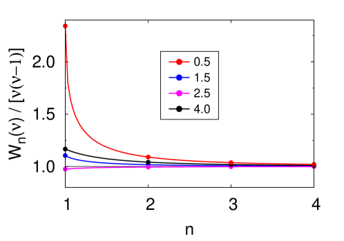
Figure 1: The function $W_{n}(\nu)$, normalized by $\nu(\nu-1)$, as a function of $n$ for the values of $\nu$ displayed in the legend. The solid lines represent expression $W_{n}(\nu)$ given by Eq. (11) with $n$ extended to the real number set.

The pathology described above can be easily cured by changing the discretization of the radial equation, replacing $a_{i}$ by $W_{n}(\nu_{i})$ in the term $a_{i}/r^{2}$. This replacement does not affect the continuum limit, and has the virtue of preserving exactly the continuum asymptotic behavior of $\tilde{u}_{i}$ as $r\rightarrow 0$ in the discrete version of the radial equation. That is, the solution of the discretized equation in the neighborhood of $r=0$ exactly reproduces the continuum result, since

$$D^{2}r_{n}^{\nu_{i}}-W_{n}(\nu_{i})r_{n}^{\nu_{i}-2}=0.$$ (13)

The replacement of the constant coefficient $a_{i}$ by $W_{n}(\nu_{i})$ in the discrete equation for $\tilde{u}_{i}$ implies that the discrete version of the original radial equation in terms of $u_{i}$ reads

$$D^{2}u_{i}(r_{n})-\sum_{j}\frac{1}{r_{n}^{2}}W_{n}^{ij}u_{j}(r_{n})-\sum_{j}U_{ij}(r_{n})u_{j}(r_{n})+\lambda u_{i}(r_{n})=0,$$ (14)

with

$$W_{n}^{ij}=\sum_{k}W_{n}(\nu_{k})v_{i}^{(k)}v_{j}^{(k)\,*},$$ (15)

where the $\vec{v}^{(k)}$, $k=1,\ldots,N_{\mathrm{e}}$, form a complete orthogonal set of eigenvectors of $A_{ij}$. Evidently, the boundary conditions remain unchanged: $u_{i}(0)=u_{i}(R)=0$.

We call the discretization scheme defined by Eq. (14) the centrifugal improved discretization (in what follows, improved discretization, to lighten the writing). The straightforward discretization has the same form, substituting $W_{n}^{ij}$ by $A_{ij}$. In what follows it is called the simple discretization.

4 The two dimensional hydrogen atom

As a test we apply the simple and improved discretization prescriptions to a simple exactly solvable case, the two dimensional hydrogen atom [16]. It describes the quantum motion of an electron constrained to move on a plane under the influence of the Coulomb potential of a point nucleus. Although at first sight it seems to be an artificial model devoid of physical interest, it has been applied to the study of impurities in very anisotropic solids [17]. The time independent Schrodinger equation in cylindric coordinates reads

$$\left[\frac{\partial^{2}}{\partial r^{2}}+\frac{1}{r}\frac{\partial}{\partial r}+\frac{1}{r^{2}}\frac{\partial^{2}}{\partial\varphi^{2}}+\frac{\xi}{r}+k^{2}\right]\psi=0$$ (16)

where $\xi=2m_{\mathrm{e}}Ze^{2}/\hbar^{2}$ and $k^{2}=2m_{\mathrm{e}}E/\hbar^{2}$, with $m_{\mathrm{e}}$ and $e$ the electron mass and charge, respectively, $Z$ the nucleus atomic number, and $E$ the energy. Negative and positive $k^{2}$ correspond to bound and scattering states, respectively. Notice that the parameter $\xi$ just sets the scale for spatial variations, and can be eliminated by rescaling the radial coordinate as $\xi r$. The wave function can be separated into the radial and angular parts as

$$\psi(r,\varphi)=\frac{u(r)}{\sqrt{r}}\mathrm{e}^{{\mathrm{i}}m\varphi},$$ (17)

with $m$ an integer, and the radial equation reads

$$u^{\prime\prime}-\frac{m^{2}-1/4}{r^{2}}u+\frac{\xi}{r}u+k^{2}u=0.$$ (18)

As $r\rightarrow 0$ the physical solution is $u=r^{\nu}[1+O(r)]$, with $\nu=1/2+|m|$. The energy of the bound states is given by the formula

$$E_{m,n_{\mathrm{r}}}=-\frac{E_{0}}{(|m|+n_{\mathrm{r}}+1/2)^{2}}$$ (19)

where $n_{\mathrm{r}}$ is a non negative integer, the radial quantum number, and the energy scale is set by $E_{0}=Z^{2}me^{4}/2\hbar^{2}$. Notice that the relation between wave number and energy can be cast to the form $E/E_{0}=4k^{2}/\xi^{2}$. Notice also that, as in the three dimensional hydrogen atom, the energy levels depend only on the principal quantum number $n=|m|+n_{\mathrm{r}}+1$, which is a positive integer. The radial functions can be expressed in terms of the confluent hypergeometric functions [16]. We are particularly interested in the ground state wave function ($m=0$, $n_{\mathrm{r}}=0$)

$$u_{0,0}(r)=2\xi^{1/2}\sqrt{\xi r}\exp(-\xi r).$$ (20)

$m$	$n_{\mathrm{r}}$	$\xi R$	$\xi\Delta$
0	0	10	0.001 – 1
0	1	40	0.01 – 1
1	0	60	0.01 – 1

Table 1: Parameters used in the computation of several bound states of the two dimensional hydrogen atom.

The radial equations (18) have been solved numerically as a numerical linear algebra eigenvalue problem using the simple and improved discretizations described in Sec. 3. The spectrum was obtained with the help of the ARPACK software package [18]. In the remaining of this section the results are briefly discussed. The parameters used in the computations are gathered in table 1. As an estimate of convergence rates we fit to the computed energy levels a power law function of the grid size $\xi\Delta$, of the form

$$\frac{E^{\mathrm{(num)}}_{\mathrm{m,n_{r}}}}{E_{0}}=\frac{E_{\mathrm{m,n_{r}}}}{E_{0}}+A(\xi\Delta)^{p},$$ (21)

where $E^{\mathrm{(num)}}_{\mathrm{m,n_{r}}}$ and $E_{\mathrm{m,n_{r}}}$ are the numerical and exact energy levels, respectively, and $A$ and $p$ are the parameters to be fit. The convergence rate is then quantified by the exponent $p$.

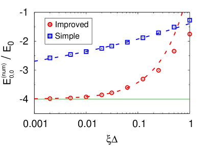
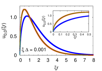
Figure 2: Left: energy of the two dimensional hydrogen atom ground state computed numerically with the simple (blue) and improved (red) discretizations of the radial equation, as a function of the discretization parameter $\xi\Delta$. The green line is the exact continuum result. The blue dashed line represents the function (21) with the parameters $A=2.61$ and $p=1/10$ obtained via a fit to the data in the range $\xi\Delta\in[0.001,0.02]$; the red dashed line corresponds to $A=3.94$ and $p=5/6$, obtained via a fit in the interval $\xi\Delta\in[0.001,0.2]$. It is apparent the extremely slow convergence rate of the simple discretization. Right: ground state radial wave function of the two dimensional hydrogen atom as a function of $\xi r$, computed numerically with the simple (blue) and improved (red) discretizations, with $\xi\Delta=10^{-3}$. The green line is the exact continuum result.

The left panel of Fig. 2 displays the lowest lying energy level, $E^{\mathrm{(num)}}_{0,0}/E_{0}$, as a function of the discretization parameter $\xi\Delta$. Notice the extremely slow convergence rate to the continuum limit, with $p=1/10$, as shown by the dashed blue line, which corresponds to a fit of Eq. (21) to the results in the range $\xi\Delta\in[0.001,0.02]$. A fit to the results of the improved discretization, displayed by the dashed red line in Fig. 2 (left), indicates that the convergence rate in this case corresponds to $p=5/6$. This is still much slower than the usual second order convergence rate, $p=2$. This slowing down can be attributed to the $1/r$ singularity of the Coulomb potential. Nevertheles, we may say that, in comparison with the simple discretization, the convergence rate of the improved discretization is extremely fast.

The right panel of Fig. 2 shows the ground state wave function computed with $\xi\Delta=10^{-3}$ with the simple (blue) and improved (red) discretizations, and the exact wave function (green line). The inset displays in detail the behavior in the vicinty of $r=0$. The wave function computed the improved discretization is indistinguisable from the exact wave function on the scale of the figure. The simple discretization gives a very inaccurate ground state wave function, even with this small value of the discretization parameter. This is due to its behavior as $r^{1/2}$ for $r\rightarrow 0$, which cannot be completely reproduced by the simple discretization in the close vicinity of the origin even though $\xi\Delta$ is very small.

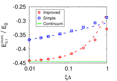
Figure 3: Left: first $m=0$ excited state ($n_{\mathrm{r}}=1$) of the two dimensional hydrogen atom computed numerically with the simple (blue) and improved (red) discretizations, versus $\xi\Delta$. The green line is the exact continuum result. The blue dashed line corresponds to the fit of (21) to the data in the interval $\xi\Delta\in[0.01,0.1]$, which gives $p=1/8$; the red dashed line is the result of a fit to the data in the range $\xi\Delta\in[0.01,0.2]$, which gives $p=7/8$. Right: lowest lying energy level with $m=1$ obtained with the simple (blue) and improved (red) discretizations. The dashed lines are fits of the function (21) to the data in the range $[0.01,0.1]$, which give $p=1.8$ for the simple discretization (blue) and $p=2$ for the improved discretization (red). The inset displays the effect of the discretization, defined as the relative difference between the result obtained with the corresponding grid and the exact continuum value.

The energy of the first excited state for $m=0$, $E^{\mathrm{(num)}}_{0,1}/E_{0}$, is displayed as a function of $\xi\Delta$ in Fig. 3 (left). Again the convergence rate is extremely slow in the case of the simple discretization, since the corresponding wave function behave as $r^{1/2}$ as $r\rightarrow 0$. Fits of Eq. (21) to the results give convergence rates with $p=1/8$ and $p=7/8$ for the simple and improved discretizations, respectively. Thus, the convergence rate is again much faster with the improved discretization than with the simple discretization. The same happens with all states with $m=0$.

For $|m|>0$ the differences between the improved and simple discretizations are not as dramatic as in the $m=0$ case. For $|m|=1$ the improved discretization converges substantially faster than the simple discretization, as can be seen in Fig. 3 (right). Fits to the results give convergence rates with $p=1.8$ for the simple discretization and $p=2$ for the improved discretization. The inset shows the relative error introduced by each discretization scheme, $|(E_{1,0}^{\mathrm{(num)}}-E_{1,0})/E_{1,0}|$, as a function of $\xi\Delta$.

For $|m|>1$ the differences between both discretizations can hardly be noticed.

5 Fluctuations around a skyrmion magnetic configuration

Radial equations appear also in the problem of determining the spectrum of fluctuations around solitonic field configurations that preserve some rotational symmetry. Examples are the t’Hooft-Polyakov monopole [19, 20], the Belavin-Polyakov instanton [21, 22] and the skyrmions [23]. Here we consider the solitonic configurations that appear in two dimensional ferromagnets with isotropic Dzyaloshinskii-Moriya interaction, which are generically called skyrmions [24].

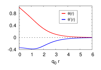
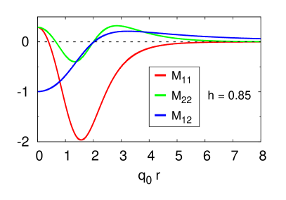
Figure 4: Left: the solitonic profile $\theta(r)$ of the magnetic skyrmion and its derivative, $\theta^{\prime}(r)$, for $h=0.85$. Right: the matrix elements $M_{\alpha\beta}(r)$ entering the skyrmion fluctuation operator for $h=0.85$.

Those magnetic skyrmions are two dimensional magnetic configurations represented by a unit vector field $\hat{n}(\vec{r})$ that point in the direction of the local magnetic moment, with unit topological charge and rotational symmetry around the magnetic field. They are stationary points of the following dimensionless energy functional

$$\mathcal{W}=\int d^{2}r\left(\frac{1}{2}\sum_{i}\partial_{i}\hat{n}\cdot\partial_{i}\hat{n}+q_{0}\hat{n}\cdot\nabla\times\hat{n}-q_{0}^{2}\vec{h}\cdot\hat{n}\right).\qquad$$ (22)

where $\partial_{i}=\partial/\partial x_{i}$, with $x_{i}\in\{x,y,z\}$ being the cartesian coordinates, $q_{0}$ is a constant with the dimensions of inverse length,

$$\hat{n}\cdot\nabla\times\hat{n}=2n_{z}(\partial_{x}n_{y}-\partial_{y}n_{x}),$$ (23)

and $\vec{h}=h\hat{z}$ is the applied magnetic field, perpendicular to the plane on which the magnetic system is confined. The skyrmion is then a solution of the Euler-Lagrange equations corresponding to the $\mathcal{W}$ functional that, using polar coordinates $(r,\varphi)$ in the plane, can be parametrized by a single function of the radial coordinate, $\theta(r)$, as [24, 13]

$$\hat{n}_{\mathrm{S}}(r,\varphi)=(\sin\theta(r)\cos\varphi,-\sin\theta(r)\sin\varphi,\cos\theta(r))$$ (24)

with the boundary conditions $\theta(0)=\pi$ and $\lim_{r\rightarrow\infty}\theta(r)=0$. Thus the skyrmion is a solitonic configuration on a ferromagnetic background that has in its center a magnetic moment opposite to the magnetic field. For $r\rightarrow\infty$, $\theta(r)$ vanishes asymptotically as $\exp(-\sqrt{h}q_{0}r)/\sqrt{q_{0}r}$. The function $\theta(r)$ is displayed as a function of $q_{0}r$ in Fig. 4 (left) for $h=0.85$.

The fluctuations around the skyrmion configuration can be parametrized by two real fields, $\xi_{\alpha}$, with $\alpha=1,2$, writing

$$\hat{n}=\left(1-\sum_{\alpha}\xi_{\alpha}^{2}\right)^{1/2}\hat{n}_{\mathrm{S}}+\sum_{\alpha}\xi_{\alpha}\hat{e}_{\alpha},$$ (25)

where $\{\hat{e}_{1},\hat{e}_{2},\hat{n}_{\mathrm{S}}\}$ form a right-handed orthonormal triad. Plugging (25) into (22) and expanding $\mathcal{W}$ in powers of $\xi_{\alpha}$, we get up to quadratic terms (the linear term vanishes on account of the Euler-Lagrange equations)

$$\mathcal{W}=\mathcal{W}(\hat{n}_{\mathrm{S}})+\int d^{2}r\sum_{\alpha\beta}\xi_{\alpha}K_{\alpha\beta}\xi_{\beta}+O(\xi^{3}),$$ (26)

where $K_{\alpha\beta}$ is a differential operator that depends on $\theta(r)$, whose explicit form is given in [13].

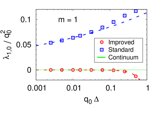
Figure 5: The eigenvalue of the skyrmion fluctuation operator corresponding to the translational zero mode ($m=1$) as a function of $q_{0}\Delta$, computed with the simple (blue) and improved (red) discretizations. The convergence rate of the simple discretization is extremely slow: the fit of (35), with $\lambda^{\mathrm{(c)}}=0$, to the data in the range $q_{0}\Delta\in[0.0025,0.02]$, represented by the blue dashed line, gives $p=1/8$. In contrast, the improved discretization shows a second order convergence rate ($p=2$), which is the result from the fit to the data (red dashed line).

The spectrum of fluctuations around the magnetic skyrmion is determined by the spectrum of $K_{\alpha\beta}$. The rotational symmetry around the magnetic field direction implies that the eigenfunctions of $K_{\alpha\beta}$ can be chosen of the form

$$\xi_{\alpha}^{(m)}(r,\varphi)=\frac{u_{\alpha}^{(m)}(r)}{\sqrt{r}}\exp({\mathrm{i}}m\varphi),$$ (27)

If $\lambda_{m}$ is the corresponding eigenvalue of $K_{\alpha\beta}$, the radial equations read

$$-u_{\alpha}^{\prime\prime}+\frac{m^{2}+3/4}{r^{2}}u_{\alpha}-\mathrm{i}\frac{2m}{r^{2}}\sum_{\beta}\epsilon_{\alpha\beta}u_{\beta}+hq_{0}^{2}u_{\alpha}+\sum_{\beta}M_{\alpha\beta}u_{\beta}=\lambda u_{\alpha},$$ (28)

where $\epsilon_{\alpha\beta}$ is the two dimensional antisymmetric tensor and, to avoid cumbersome notation, the index $m$ in $u_{\alpha}$ and $\lambda$ is not explicitely shown. The matrix $M_{\alpha\beta}$, which is analytic in $r=0$ and vanishes exponentially as $r\rightarrow\infty$, is

$$M_{11} = -2\frac{\sin^{2}\theta}{r^{2}}-2q_{0}\frac{\sin(2\theta)}{r}+hq_{0}^{2}(\cos\theta-1),$$ (29)

$$M_{22} = -\frac{\sin^{2}\theta}{r^{2}}-q_{0}\frac{\sin(2\theta)}{r}-\theta^{\prime}(\theta^{\prime}+2q_{0})+hq_{0}^{2}(\cos\theta-1),$$ (30)

$$M_{12} = \mathrm{i}2m\left(\frac{1+\cos\theta}{r^{2}}-q_{0}\frac{\sin\theta}{r}\right),$$ (31)

and $M_{21}=-M_{12}$. The boundary conditions are $u_{\alpha}(0)=0$ and, for bound states, $u_{\alpha}(R)=0$, with $R\rightarrow\infty$. For scattering states the boundary condition is related to the oscillatory behavior of the wave function as $r\rightarrow\infty$, although we may consider the system enclosed in a box of radius $R$, so that $u_{\alpha}(R)=0$, and let $R\rightarrow\infty$. Notice that $q_{0}$ merely sets the scale of spatial variations and can be eliminated by a rescaling of the radial coordinate. Hence, the eigenfunctions depend on $q_{0}r$ and the eigenvalues are proportional to $q_{0}^{2}$. The functions $M_{\alpha\beta}$ are displayed in Fig. 4 (right), as a function of $q_{0}r$ for $h=0.85$.

The asymptotic form of Eq. (28) for $r\rightarrow 0$ gives the matrix $A_{ij}$:

$$A=\left(\begin{array}[]{cc}m^{2}+3/4&-{\mathrm{i}}2m\\ {\mathrm{i}}2m&m^{2}+3/4\end{array}\right).$$ (32)

Its eigenvalues are $a_{\pm}=(m\pm 1)^{2}-1/4$, and therefore the behaviour of the physical solution $u_{\alpha}$ (regular at $r=0$) as $r\rightarrow 0$ is given by

$$\nu_{\pm}=1/2+|m\pm 1|.$$ (33)

Due to the translational invariance of the skyrmion, the operator $K_{\alpha\beta}$ has two independent normalizable (bound states) zero modes, which have $m=\pm 1$. For the case $m=+1$, its two components are

$$\begin{array}[]{ll}u_{1}(r)=-\sqrt{r}\theta^{\prime}(r),\\ \\ u_{2}(r)=-\sin\theta(r)/\sqrt{r}.\end{array}$$ (34)

The discretization breaks the continuous translational symmetry and the discretized operator does not have exact zero modes: the eigenvalues of the bound states with $m=\pm 1$ tend to zero in the continuum limit.

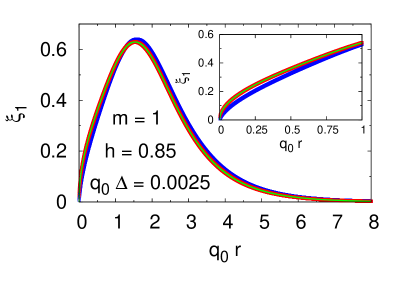
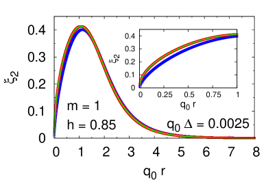
Figure 6: Components of skyrmion fluctuation zero mode eigenfunction ($m=1$) for $h=0.85$, obtained with the improved (red) and simple (blue) discretizations, with $q_{0}\Delta=0.0025$. The green line is the exact continuum result. The insets show magnifications of the $r=0$ vicinity.

The continuum spectrum has a gap of magnitude $q_{0}^{2}h$, so that it appears for $\lambda\geq q_{0}^{2}h$. The discrete spectrum, which depends qualitatively on $h$, is located below the gap, $\lambda<q_{0}^{2}h$. In addition to the zero mode, there is one bound state with $m=0$ (a breathing mode) for any $h$. For $h<0.98$ two (degenerate) bound states with $m=\pm 2$ appear. Succesive bound states with correlative higher values of $|m|$ arise by lowering $h$. For $h<0.57$ the eigenvalue of the $|m|=2$ bound states is negative and therefore the skyrmion is unstable.

The bound states have been computed by numerical diagonalization, with the ARPACK software package [18], of the operator (28) discretized with the simple and improved schemes. To estimate the convergence rates we fit to the computed eigenvalues a power law function of the grid size $q_{0}\Delta$, of the form

$$\lambda/q_{0}^{2}=\lambda^{\mathrm{(c)}}+A(q_{0}\Delta)^{p},$$ (35)

where $\lambda^{\mathrm{(c)}}$, $A$, and $p$ are the parameters to be fit. Evidently, $\lambda^{\mathrm{(c)}}$ is an extrapolation of the results to the continuum limit. The convergence rate is quantified by the exponent $p$.

Let us discuss the results for the typical case $h=0.85$, for which we set $q_{0}R=25$. Fig. 5 displays the computed eigenvalue of the $m=1$ bound state, which becomes a zero mode in the continuum limit, as a function of the discretization parameter $q_{0}\Delta$. Notice the extremely slow convergence rate in the case of the simple discretization: a fit of the function (35), with $\lambda^{\mathrm{(c)}}=0$, to the data gives $p=1/8$. It is represented by the blue dashed line. In comparison, the convergence rate with the improved discretization is extremly fast: the fit gives $p=2$. The fact that the convergence rate of the improved discretization in the skyrmion problem is of the expected second order contrasts with the much slower convergence rate in the case of the 2D hydrogen atom. This is likely due to the fact that the potential of the skyrmion fluctuations is analytic at $r=0$, while it is coulombian ($1/r$) in the case of the hydrogen atom.

	Simple			Improved
$m$	$\lambda^{\mathrm{(c)}}$	$A$	$p$	$\lambda^{\mathrm{(c)}}$	$A$	$p$
0	0.3561	-0.101	2	0.3561	-0.057	2
1	–	0.113	1/8	–	-0.048	2
2	0.5987	-0.232	2	0.5987	-0.100	2

Table 2: Results of the fits of the function (35) to the numerical results for the bound state spectrum of skyrmion fluctuations with $h=0.85$.

The components of the zero mode eigenfunction with $m=1$ are displayed in Fig. 6 for $q_{0}\Delta=0.0025$. The insets are a magnification of the vicinity of $r=0$. The green lines are the exact continuum results given by Eqs. (34). In the scale of the figure they are indistinguisable from the eigenfunction components computed with the improved discretization; in the case of the simple discretization there are noticeably differences.

The convergence rate with the improved discretization is also faster for the other two bound states ($m=0$ and $m=2$), as shown in Figs. 7, left and right, respectively. The improvement, however, is not as dramatic as for the zero mode. The reason is that the zero mode behaves in the vicinity of $r=0$ as $r^{1/2}$, while the other two bound states behave as $r^{3/2}$. Indeeed, in both discretizations the convergence rate is described by the exponent $p=2$ that corresponds to second order convergence. The results of fits of (35) to the data are gathered in table 2. Notice that the extrapolations to the continuum limit given by both discretizations agree to a high accuracy. The insets in Figs. 7 display the effect of the discretization, defined as the difference between the eigenvalue computed in the corresponding grid and the continuum limit, estimated through the extrapolation $\lambda^{\mathrm{(c)}}$.

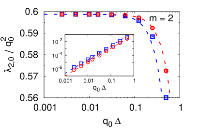
Figure 7: Eigenvalue of the skyrmion fluctuation bound states $m=0$ (left) and $m=2$ (right) for $h=0.85$, obtained with the improved (red circles) and simple (blue squares) discretizations, versus the discretization parameter $q_{0}\Delta$. The dashed lines represents the fits of (35) to the data in the interval $q_{0}\Delta\in[0.0025,0.02]$. In all cases they are compatible with second order convergence ($p=2$). The insets display the effect of the discretization, defined as the difference between the eigenvalue computed in the corresponding grid and the continuum limit, estimated through the extrapolation $\lambda^{\mathrm{(c)}}$ (table 2).

6 Conclusions

The simplest central difference discretization of the second derivative of a function converges very slowly to the continuum limit at points where the function is singular in such a way that its fourth derivative becomes very large. This happens in some instances of radial equations, depending on the coefficient of the $1/r^{2}$ term, which usually represents the centrifugal potential. In such cases, the solution of the radial equation through the diagonalization of the discretized equation converges to the continuum limit at an extremely slow rate. This problem is caused by the singular nature of the function and is not cured by a higher order discretization of the second derivative. The convergence is extraordinarily accelerated if the $1/r^{2}$ term is discretized in such a way that the form of the continuum solution in the vicinity of the origin is exactly reproduced in the discretized problem. We call this finite differences scheme the centrifugal improved discretization.

The centrifugal improved discretization is relevant in two dimensional problems, where the radial function behaves as $r^{\nu}$ for $r\rightarrow 0$, with the exponent $\nu$ non-integer. This is typical of two dimensional problems. In three dimensional problems $\nu$ is always an integer if the potential is regular, $\lim_{r\rightarrow 0}r^{2}V(r)=0$, since in this case the $1/r^{2}$ term represents the centrifugal potential. However, for transition potentials, defined as those for which $\lim_{r\rightarrow 0}r^{2}V(r)=g$ is a real non-zero number [14], the exponent $\nu$ is in general not an integer. In the limiting case $g\rightarrow-1/4$, $\nu=1/2$. The method presented in this paper is thus very well suited for the numerical study of transition potentials, which show very special theoretical features [14]. The simplest transition potential, the inverse square potential, $V(r)=g/r^{2}$, has been extensively studied as it is exactly solvable (see for instance [25]). Transition potentials are not just theoretically interesting, but have many physical applications. For instance, the potential due to a dipole is of inverse square type and has been applied long ago to the capture of electrons by polar molecules [26]. Other experimental realizations of the inverse square potential and its associated phenomenology have also been reported [27, 28].

For singular potentials, defined as those that are more singular than $1/r^{2}$, the behaviour of the radial function at the origin is not determined by the $1/r^{2}$ term but by the most singular term of the potential. For these cases, an improved finite differences scheme analogous to the centrifugal improved discretization can be devised, discretizing the potential in such a way that the form of the radial function as $r\rightarrow 0$ is exactly reproduced by the discretized solution. This prescription will provide a powerful tool to study singular potentials, which are not just academic problems, since they appear in many physical systems. For instance, the potential interaction between one polar and one non-polar molecule is of $1/r^{4}$ type.

Finally, the centrifugal improved discretization can be also used to find numerically symmetric solutions of nonlinear equations provided that the nonlinearity does not alter the singular behavior at the origin. An instance is the Gross-Pitaevskii equation [29, 30] with cylindric symmetry, in which the nonlinear term in the radial equation has the form $u^{3}/r^{3/2}$, so that the most singular term at the origin is the centrifugal potential. A relaxation method can be used to solve the discretized nonlinear equation.

The authors acknowledge the Grant No. MAT2015-68200-C2-2-P from the Spanish Ministry of Economy and Competitiveness. This work was partially supported by the scientific JSPS Grant-in-Aid for Scientific Research (S) (Grant No. 25220803), and the MEXT program for promoting the enhancement of research universities, and JSPS Core-to-Core Program, A. Advanced Research Networks.

References

- [1] L. Landau and E. Lifchitz. Mécanique Quantique. Editions MIR, Moscou, 1974.
- [2] A. Sommerfeld. Partial Differential Equations in Physics. Academic Press Inc., New York, 1949.
- [3] G.H. Rawitscher and I. Koltracht. An efficient numerical spectral method for solving the Schrödinger equation. Computing in Science and Engineering, 7:58–66, 2005.
- [4] D.D. Morrison, J.D. Riley, and J.F. Zancanaro. Multiple shooting method for two-point boundary value problems. Communications of the ACM, 12:613–614, 1962.
- [5] J. Killingbeck. Shooting methods for the Schrödinger equation. Phys. A: Math. Gen., 20:1411–1418, 1987.
- [6] D.P. Sakas and T.E. Simos. Multiderivative methods of eighth algebraic order with minimal phase-lag for the numerical solution of the radial Schrödinger equation. Journal of Computational and Applied Mathematics, 175:161–172, 2005.
- [7] Qinghe Ming, Yanping Yang, and Yonglei Fang. An optimized runge-kutta method for the numerical solution of the radial Schrödinger equation. Mathematical Problems in Engineering, 2012:867948, 2012.
- [8] Yonglei Fang, Xiong You, and Qinghe Ming. A new phase-fitted modified runge–kutta pair for the numerical solution of the radial Schrödinger equation. Applied Mathematics and Computation, 224:432–441, 2013.
- [9] V. Fack and G. Vanden Berghe. A program for the calculation of energy eigenvalues and eigenstates of a Schrödinger equation. Computer Physics Communications, 39:187–196, 1986.
- [10] T.E. Simos and P.S. Williams. On finite difference methods for the solution of the Schrödinger equation. Computers & Chemistry, 23:513–554, 1999.
- [11] J. Vigo-Aguiar and T.E. Simos. Review of multistep methods for the numerical solution of the radial Schrödinger equation. International Journal of Quantum Chemistry, 103:278–290, 2005.
- [12] LLoyd N. Trefethen. Spectral Methods in Matlab. SIAM, Philadelphia, 2000.
- [13] V. Laliena and J. Campo. Stability of skyrmion textures and the role of thermal fluctuations in cubic helimagnets: a new intermediate phase at low temperature. Physical Review B, 96:134420, 2017.
- [14] W.M. Frank, D.J. Land, and R.M. Spector. Singular potentials. Review of Modern Physics, 43:36––98, 1971.
- [15] L. A. Toikka, J. Hietarinta, and K.-A. Suominen. Exact soliton-like solutions of the radial Gross–-Pitaevskii equation. J. Phys. A: Math. Theor., 45:48203, 2012.
- [16] X.L. Yang, S.H. Guo, F.T. Chan, K.W. Wong, and W.Y. Ching. Analytic solution of a two dimensional hydrogen atom. i. nonrelativistic theory. Physical Review A, 43:1186–1196, 1991.
- [17] W. Kohn and J.M. Luttinger. Theory of donor states in silicon. Physical Review, 98:915–922, 1955.
- [18] R.B. Lehoucq, D.C. Sorensen, and C. Yang. ARPACK Users Guide: Solution of Large-Scale Eigenvalue Problems with Implicitly Restarted Arnoldi Methods. SIAM, Philadelphia, 1998.
- [19] G. ’t Hooft. Magnetic monopoles in unified gauge theories. Nuclear Physics B, 79:276–284, 1974.
- [20] A.M. Polyakov. Particle spectrum in the Quantum Field Theory. JETP Letters, 20:194–196, 1974.
- [21] A.A. Belavin and A.M. Polyakov. Metastable states of two dimensional isotropic ferromagnets. JETP Letters, 22:246–247, 1975.
- [22] B.A. Ivanov, D.D. Sheka, V.V. Krivonos, and F.G. Mertens. Quantum effects for the 2D soliton in isotropic ferromagnets. Physical Review B, 75:132401, 2007.
- [23] T. H. R. Skyrme. A non-linear field theory. Proceedings of the Royal Society A, 260:127–138, 1961.
- [24] A. Bogdanov and A. Hubert. Thermodynamically stable magnetic vortex states in magnetic crystals. Journal of Magnetism and Magnetic Materials, 138:255–269, 1994.
- [25] H. Camblong, L.N. Epele, H. Fanchiotti, and C.A. Garcia Canal. Renormalization of the inverse square potential. Physical Review Letters, 85:1590, 2000.
- [26] J.-M. Lévy-Leblond. Electron capture by polar molecules. Physical Review, 153:1––4, 1967.
- [27] C. Desfrançois, H. Abdoul-Carime, N. Khelifa, and P. Schermann. From to potentials: Electron exchange between Rydberg atoms and polar molecules. Physical Review Letters, 73:2436––2439, 1994.
- [28] J. Denschlag, G. Umshaus, and J. Schmiedmayer. Probing a singular potential with cold atoms: A neutral atom and a charged wire. Physical Review Letters, 81:737––741, 1998.
- [29] E. P. Gross. Structure of a quantized vortex in boson systems. Il Nuovo Cimento, 20:454–457, 1961.
- [30] P.P. Pitaevskii. Vortex lines in an imperfect bose gas. Soviet Physics JETP, 13:451–454, 1961.