Abstract

Diffusion to capture is an ubiquitous phenomenon in many fields in biology and physical chemistry, with implications as diverse as ligand-receptor binding on eukaryotic and bacterial cells, nutrient uptake by colonies of unicellular organisms and the functioning of complex core-shell nanoreactors. Whenever many boundaries compete for the same diffusing molecules, they inevitably shield a variable part of the molecular flux from each other. This gives rise to the so-called diffusive interactions (DI), which can reduce substantially the influx to a collection of reactive boundaries depending chiefly on their geometrical configuration.
In this review we provide a pedagogical discussion of the main mathematical aspects underlying a rigorous account of DIs. Starting from a striking and deep result on the mean-field description of ligand binding to a receptor-covered cell, we develop little by little a rigorous mathematical description of DIs in the stationary case through the use of translational addition theorems for spherical harmonics. We provide several enlightening illustrations of this powerful mathematical theory, including diffusion to capture to ensembles of reactive boundaries within a spherical cavity.

Index type ‘default’ not definedI can’t help

Chapter 0 Diffusion to capture and the concept of diffusive interactions

Contents

1. 0 Diffusion to capture by many competing boundaries
   1. 1 Introduction
   2. 2 Bimolecular diffusive encounters as two-body boundary problems
      1. 1 Finite reaction probability and radiation boundary conditions
   3. 3 Approximate evaluation of diffusive interactions: a surprising lesson in biology
   4. 4 The generalized method of separation of variables allows one to solve the problem semi-analytically
      1. 1 Diffusive interactions between two spheres
      2. 2 Diffusive interactions are weaker among multiple partially reactive boundaries
   5. 5 Many spherical boundaries arranged arbitrarily in space
      1. 1 Many spheres inside a spherical cavity
   6. 6 Summary
   7. 1 The solution to the problem
   8. 2 The rate

1 Introduction

It is common knowledge that the first step of any chemical or biochemical reaction proceeding in an inert fluid phase is the mutual diffusive encounter of reactants [1]

$${{{{\mathrm{\mathrm{A}}}}+{}{{\mathrm{\mathrm{B}}}}{{}\mathrel{\hbox to0.0pt{\raisebox{0.94722pt}{$\ext@arrow 3399\arrowfill@\relbar\relbar\rightharpoonup{}{\mathchoice{\mathchoice{\mbox{$\displaystyle\kappa_{\rm on}(t)$}}{\mbox{$\textstyle\kappa_{\rm on}(t)$}}{\mbox{$\scriptstyle\kappa_{\rm on}(t)$}}{\mbox{$\scriptscriptstyle\kappa_{\rm on}(t)$}}}{\mathchoice{\mbox{$\displaystyle\kappa_{\rm on}(t)$}}{\mbox{$\textstyle\kappa_{\rm on}(t)$}}{\mbox{$\scriptstyle\kappa_{\rm on}(t)$}}{\mbox{$\scriptscriptstyle\kappa_{\rm on}(t)$}}}{\mathchoice{\mbox{$\displaystyle\kappa_{\rm on}(t)$}}{\mbox{$\textstyle\kappa_{\rm on}(t)$}}{\mbox{$\scriptstyle\kappa_{\rm on}(t)$}}{\mbox{$\scriptscriptstyle\kappa_{\rm on}(t)$}}}{\mathchoice{\mbox{$\displaystyle\kappa_{\rm on}(t)$}}{\mbox{$\textstyle\kappa_{\rm on}(t)$}}{\mbox{$\scriptstyle\kappa_{\rm on}(t)$}}{\mbox{$\scriptscriptstyle\kappa_{\rm on}(t)$}}}}$}\hss}\raisebox{-0.94722pt}{$\ext@arrow 3399\arrowfill@\leftharpoondown\relbar\relbar{k_{\rm off}}{\hphantom{\kappa_{\rm on}(t)}}$}}{}{}}{{\mathrm{\mathrm{A}}\nolinebreak{\cdot}\mathrm{\mathrm{B}}}}{{}\mathrel{\hbox to0.0pt{\raisebox{0.94722pt}{$\ext@arrow 3399\arrowfill@\relbar\relbar\rightharpoonup{}{\mathchoice{\mathchoice{\mbox{$\displaystyle\hskip 10.00002pt$}}{\mbox{$\textstyle\hskip 10.00002pt$}}{\mbox{$\scriptstyle\hskip 10.00002pt$}}{\mbox{$\scriptscriptstyle\hskip 10.00002pt$}}}{\mathchoice{\mbox{$\displaystyle\hskip 10.00002pt$}}{\mbox{$\textstyle\hskip 10.00002pt$}}{\mbox{$\scriptstyle\hskip 10.00002pt$}}{\mbox{$\scriptscriptstyle\hskip 10.00002pt$}}}{\mathchoice{\mbox{$\displaystyle\hskip 10.00002pt$}}{\mbox{$\textstyle\hskip 10.00002pt$}}{\mbox{$\scriptstyle\hskip 10.00002pt$}}{\mbox{$\scriptscriptstyle\hskip 10.00002pt$}}}{\mathchoice{\mbox{$\displaystyle\hskip 10.00002pt$}}{\mbox{$\textstyle\hskip 10.00002pt$}}{\mbox{$\scriptstyle\hskip 10.00002pt$}}{\mbox{$\scriptscriptstyle\hskip 10.00002pt$}}}}$}\hss}\raisebox{-0.94722pt}{$\ext@arrow 3399\arrowfill@\leftharpoondown\relbar\relbar{}{\hphantom{\hskip 10.00002pt}}$}}{}}...{{}\mathrel{\hbox to0.0pt{\raisebox{0.94722pt}{$\ext@arrow 3399\arrowfill@\relbar\relbar\rightharpoonup{}{\mathchoice{\mathchoice{\mbox{$\displaystyle\hskip 10.00002pt$}}{\mbox{$\textstyle\hskip 10.00002pt$}}{\mbox{$\scriptstyle\hskip 10.00002pt$}}{\mbox{$\scriptscriptstyle\hskip 10.00002pt$}}}{\mathchoice{\mbox{$\displaystyle\hskip 10.00002pt$}}{\mbox{$\textstyle\hskip 10.00002pt$}}{\mbox{$\scriptstyle\hskip 10.00002pt$}}{\mbox{$\scriptscriptstyle\hskip 10.00002pt$}}}{\mathchoice{\mbox{$\displaystyle\hskip 10.00002pt$}}{\mbox{$\textstyle\hskip 10.00002pt$}}{\mbox{$\scriptstyle\hskip 10.00002pt$}}{\mbox{$\scriptscriptstyle\hskip 10.00002pt$}}}{\mathchoice{\mbox{$\displaystyle\hskip 10.00002pt$}}{\mbox{$\textstyle\hskip 10.00002pt$}}{\mbox{$\scriptstyle\hskip 10.00002pt$}}{\mbox{$\scriptscriptstyle\hskip 10.00002pt$}}}}$}\hss}\raisebox{-0.94722pt}{$\ext@arrow 3399\arrowfill@\leftharpoondown\relbar\relbar{}{\hphantom{\hskip 10.00002pt}}$}}{}}{{\mathrm{\mathrm{P}}}}}}$$ (1)

In the above general scheme, the encounter complex $A\cdot B$ is transformed reversibly into a (series of) products (collectively indicated by $P$), through a variable number of intermediate steps that depend on the specific reaction considered. Irrespectively of whether the reaction (1) is considered under thermodynamical equilibrium or non-equilibrium conditions, the second-order rate constant $\kappa_{\rm on}$ is proportional to the effective relative diffusion coefficient of the species $A$ and $B$ and describes the formation of the encounter complex. For this reason, these kind of reactions are also known in the physical chemistry community with the term diffusion-influenced reactions. The time dependence of $\kappa_{\rm on}$ refers to the possibility of investigating transient kinetics effects as opposed to steady-state (equilibrium or non-equilibrium) kinetics.
Several mathematical difficulties emerge when one tries to develop a general kinetic theory of bulk irreversible diffusion-influenced reactions. One way around this problem is to treat trapping and target models [2], which are simpler than the original one. In the first model a particle, say, $B$ diffuses towards many sinks $A$ that are often assumed to be static. Conversely, the target problem describes a situation where many sinks $A$ diffuse to a static particle $B$ [3]. The two settings, even if equivalent under certain conditions (see Ref. 2), describe in general different problems at high density of reactants. In the present paper, we shall concentrate on the trapping model for reactions of the kind (1).
Diffusion in domains with one-connected smooth boundaries is a fairly well-understood and well-characterized phenomenon from the general standpoint of mathematical physics [4]. However, real-life situations are often very complex and make mathematical descriptions challenging. For example, this is the case of biochemical reactions taking place in living media, such as the cell interior or the extra-cellular matrix (e.g. paracrine delivery) [5], where confinement, crowding (excluded-volume) effects [6, 7] and non-specific interactions among diffusing species and with all sorts of cellular structures [8] make it very difficult to elaborate quantitative models for the calculation of diffusive encounter rates [9, 10, 11, 12, 13].
Among all the possible effects on diffusion-influenced encounters and reactions arising in non-ideal conditions, in this short review we shall concentrate on the so-called diffusive interactions (DI). As we shall see in the following, these describe a fundamental mechanism of competition among different reactive boundaries, competing for the same diffusive molecular flux. This effect was discussed for the first time as far back as 1953 by Frisch and Collins in terms of a competition phenomenon [14]. A decade later, Reck and Prager referred to the same phenomenon simply as an interaction [15]. Although the same problem has been investigated later in different contexts, it seems that there is invariably a reference to a generic competition mechanism [16, 17], until the term diffusive interactions was introduced by Traytak [18] in analogy with hydrodynamical interactions for Stokes flow in many-body systems.
Picture for example a concentration field of small ligand molecules (e.g. signaling hormones or growth factors) diffusing in the extra-cellular matrix or in the bacterial periplasm looking for an available receptor on a cell membrane to form a complex. For the sake of the argument, let us imagine that far away from the receptor-covered surface the ligand bulk concentration is constant and that the ligand-receptor affinity is large enough to consider receptors as sinks, i.e. perfectly absorbing units. H. Berg has famously termed this general scheme of diffusive problems diffusion to capture [19]. If the surface density of receptors is low, then the diffusion problem is additive and the overall capture rate for the whole ensemble of receptors (e.g. number of ligands diffusing to a receptor per unit time) is well estimated by the sum of the individual rates. In this case, a many-body problem can be solved as many identical two-body problems. However, receptors on cell membranes are typically very densely packed in clusters [20, 21, 22, 23, 24, 25, 26]. In this case, any two identical receptors sitting at close separation will screen a portion of the diffusive ligand flux to each other. Overall, a complex pattern of many-body screening effects will arise, reflecting the many-body geometrical arrangement of receptors, with the consequence of reducing the overall capture rate corresponding to the array of receptors. A similar scenario is relevant for the case of multivalent molecules, i.e molecules carrying more than one binding sites [27, 28, 29, 30, 31]. By the same token, diffusive interactions among the different active sites will give rise to a similar negative cooperativity, which will reduce the overall capture rate with respect to an equivalent number of isolated sites.
Mathematically, if many-body effects are relatively well characterized for unbounded systems of distributed sinks [32, 33, 34, 35, 2, 36, 37], the case of diffusive interactions for sinks or partially absorbing boundaries located in a finite domain is more challenging from a mathematical standpoint. This scenario is relevant in many fields, ranging from catalysis in composite nanostructures [38, 39, 40] to nutrient uptake by dense colonies of microorganisms [41].
A full treatment of time-dependent diffusive interactions is extremely hard to treat and de facto limited to simple cases [42, 43]. Conversely, several methods have been used to tackle this problem for different geometries in the stationary state, where more theoretical approaches are available, such as renormalization group [18, 44] and the method of irreducible Cartesian tensors [18] and the generalized method of separation of variables [45, 46], based on addition theorems for solid harmonics [47, 48, 45, 46]. It is also possible to combine such methods with methods based on dual-series relations [49] to deal with the case of diffusive interactions among inhomogeneous reactive boundaries with active and reflecting patches [50, 51, 52].
In this short review, we will provide a concise account of DI arising in many-body systems consisting of spherical fully absorbing and partially absorbing boundaries within a finite domain. In s:1 we will lay out the basic ideas of the mathematical method employed to compute the diffusive encounter rate for two isolated spherical molecules. In s:2, these ideas will be used to estimate many-body effects in the mean-field approximation and illustrate the main physical features of DI. In s:3, we will show how using multipole expansion methods coupled to translational addition theorems for solid harmonics allows one to solve the problem exactly to any desired level of accuracy for arbitrary geometries. This method constitutes a powerful tool that can be employed to tackle a wide host of important problems in physical chemistry and biology.

2 Bimolecular diffusive encounters as two-body boundary problems

The polish physicist Marian Ritter von Smolan Smoluchowski (1872-1917), besides being a skilled water-color painter and an exquisite pianist, during the first two decades of the XX century laid the bases of the mathematical theory of diffusion processes [53, 54]. The calculation of diffusive encounter rates in ideal conditions follows directly from his ideas. Let us imagine a solution containing two spherical molecules $A$ and $B$, with radii $R_{A}$ and $R_{B}$, diffusion coefficients $D_{A}$ and $D_{B}$ and concentrations (number densities) $c_{A}$ and $c_{B}$. Our goal is to determine the rate of $A$-$B$ encounters dictated by their relative diffusive motion as a function of the concentrations. The full many-body problem is exceedingly hard to treat analytically. However, as it was first recognized by Smoluchowski, one can reduce it to the effective two-body problem of relative diffusion of a single A-B pair under certain hypotheses. However, as already noted by Szabo [55], the commonly accepted hypothesis of high dilution of both species is not enough. The first step towards the equivalent two-body problem is that one species be much more diluted than the other. Yet, not even this is enough. Let us imagine that the particles of kind $A$ are sufficiently diluted, i.e. $c_{A}\ll c_{B}$, so that one can concentrate on a single $A$ particle surrounded by many $B$ particles, say $N$ of them. It is not difficult to show that the $(N+1)$-body Smoluchowski equation describing the diffusion of a single $A$ molecule within a sea of $B$ particles contains cross-terms that make it non-separable if $D_{A}\neq 0$ [2]. Therefore, bimolecular encounters between $A$ and $B$ molecules can be modeled as an equivalent two-body problem provided that

Both species should be highly diluted, so that mutual interactions can be safely neglected.

One species ($A$) must be much more diluted than the other, so that the full problem can be reduced to study the fate of a single particle surrounded by many particles of the other species.

The diffusion coefficient of the highly diluted species should be much smaller than that of the other species (from $N$-body to two-body). A consequence of this is that the relative diffusion coefficient essentially coincides with the one of the mobile species, i.e. $D=D_{A}+D_{B}\simeq D_{B}$. Under these conditions the rate of encounters can be computed by solving the following stationary diffusion problem (i.e. Laplace equation) for the local concentration field $c(\boldsymbol{r})$ of $B$ molecules.

$$\nabla^{2}c=0$$ (2a)

$$c|_{\partial\Omega}=0$$ (2b)

$$\lim_{r\to\infty}c=c_{B}$$ (2c)

This describes to the non-equilibrium steady state arising as a constant bulk concentration $c_{B}$ is maintained far from the reactive boundary $\partial\Omega$, which acts as a perfectly absorbing sinks. This is the contact surface of the two molecules, which is the sphere $\mathcal{S}_{R}$ of radius $R=R_{A}+R_{B}$, since both $A$ and $B$ molecules are spherical by assumption. Physically, this describes the pseudo-first order (annihilation) reaction

$$A+B\stackrel{{\scriptstyle\kappa_{S}}}{{\to}}A$$

whose rate $k_{S}=\kappa_{S}c_{B}$ coincides with the overall flux into the reactive surface $\mathcal{S}_{R}$, i.e. the number of $B$ molecules crossing $\mathcal{S}_{R}$ per unit time. Here, we shall use the Greek letter $\kappa$ to denote rate constants (dimensions of inverse concentration times inverse time) and the Latin letter $k$ to denote rates (dimensions of inverse time). The rate can be computed straightforwardly as the incoming flux across $\mathcal{S}_{R}$, that is

$$k_{S}=-\int_{\mathcal{S}_{R}}\boldsymbol{J}\cdot\hat{\boldsymbol{n}}\,dS$$ (3)

where $\boldsymbol{J}=-D\nabla c$ is the relative diffusion current (Fick’s first law).
The solution to the spherically symmetric boundary problem (2) can be computed straightforwardly, yielding

$$c(r)=c_{B}\left(1-\frac{R}{r}\right)$$ (4)

which, using e:flux, immediately gives the so-called Smoluchowski rate constant $\kappa_{S}$

$$\kappa_{S}=4\pi DR$$ (5)

The rate of encounter is thus $k_{S}=4\pi DRc_{B}$ molecules per unit time disappearing across the absorbing boundary $\mathcal{S}_{R}$. Note that this is proportional to the linear size of the latter, a distinctive signature of the diffusive dynamics.

1 Finite reaction probability and radiation boundary conditions

The scheme (2) describes the reactive boundary as a perfect sink, which amounts to consider that $B$ particles are annihilated the moment they reach contact distance. This is meant to describe a (long-lived) binding event. However, in reality the two reacting partners first approach diffusively to contact distance forming the so-called encounter complex. Subsequently, this can either dissociate (this is the case if for example the two partners were not mutually oriented in a favourable manner) or proceed to form a stable contact. This more realistic situation can be accommodated for within the above mathematical formalism thanks to an intuition put forward by Collins and Kimball in 1949 [56]. The idea is to replace the perfectly absorbing boundary condition (2b) with a radiation boundary condition (in more mathematical terms Robin boundary condition), that interpolates between perfectly absorbing (Dirichlet type) and perfectly reflecting (von Neumann type) boundary conditions. Namely, the boundary value problem (2) is replaced by

$$\nabla^{2}c=0$$ (6a)

$$\left.\left(4\pi DR^{2}\frac{\partial c}{\partial r}-\kappa^{\ast}c\right)\right|_{\partial\Omega}=0$$ (6b)

$$\lim_{r\to\infty}c=c_{B}$$ (6c)

The boundary condition (6b) stipulates that the particle flux across the reactive contact surface is proportional to the local concentration of ligands $B$. The proportionality constant, the intrinsic rate constant $\kappa^{\ast}$, can be considered as describing the physical mechanism underlying the chemical fixation of the encounter complex. In the limit $\kappa^{\ast}\to 0$, the surface becomes perfectly reflecting, i.e. no reaction can occur. In the opposite limit, $\kappa^{\ast}\to\infty$ (mathematically, it is necessary to divide e:SmolBPrbc2 by $\kappa^{\ast}$ before taking the limit) one recovers the perfectly absorbing boundary, which is thus seen as corresponding to infinitely fast chemical fixation step. As we shall see, the latter case is known as the diffusion-limited regime, where the diffusive encounter is the rate-limiting step of the reaction. Diffusion-limited is as-fast-as-one-can-go, other situations corresponding to a finite intrinsic reaction rate necessarily proceeding slower than that.
The solution to the problem (6) can be computed as straightforwardly as before, yielding

$$c(r)=c_{B}\left[1-\left(\frac{h}{1+h}\right)\frac{R}{r}\right]$$ (7)

where $h=\kappa^{\ast}/\kappa_{S}$, which, using e:flux, gives

$$\kappa=\kappa_{S}\left(\frac{h}{1+h}\right)$$ (8)

In general, $\kappa<\kappa_{S}$. This case in the physical chemistry community is often indicated with the specific term diffusion-influenced regime (or reaction), as opposed to the diffusion-limited regime, $h\to\infty$, where $\kappa=\kappa_{S}$.

3 Approximate evaluation of diffusive interactions: a surprising lesson in biology

The concept of diffusive interactions is best introduced through a simple, yet astonishing classical result. Let us consider a cell, which we model as a spherical surface of radius $R$, uniformly covered with $M$ receptors, which we model as small absorbing circular patches of radius $a$. The rest of the cell surface is supposed to be reflecting. The problem of computing the rate of absorption of this partially absorbing cell was first famously considered by Berg and Purcell in 1977 [57]. Here, we shall follow the appealing re-derivation by Shoup and Szabo [58] of the same result. The main idea is to treat the receptor-covered cell as a partially absorbing sphere, in the sense of radiation boundary conditions. According to Shoup and Szabo’s argument, the corresponding intrinsic reaction rate constant can be computed as the ratio between the rate constant of $M$ isolated circular disks on an otherwise reflecting surface and the Smoluchowski rate constant of the entire cell, namely

$$\kappa^{\ast}=4Da\times M$$ (9)

where we used the classical result $k_{a}=4Da$ for the rate constant of a small absorbing disk on an infinite reflecting plane [59]. Using e:Smolk, the rate constant corresponding to the partially absorbing sphere is easily found, namely

$$\kappa=\kappa_{S}\left(\frac{Ma}{\pi R+Ma}\right)$$ (10)

A surprising finding emerges if we plug realistic figures in e:SSkcell. The typical size of a cell is around $10$ $\mu$m, while the typical size of a receptor is of the order of $1.5$ nm. If we calculate how many receptors are needed to reduce the rate constant to only one half that of the fully covered cell, i.e. $\kappa_{S}$, we find $M\simeq 10^{4}$, which is the correct order of magnitude for the average number of receptors of a given family present on a cell’s surface at any given time [60]. Is this a large number? A quick calculation shows that the fraction of cell surface covered by as many receptors is $\simeq 10^{-4}$ ! To summarize, an active surface fraction as low as $10^{-4}$ only yields a factor of 2 reduction in the rate of capture. The surprising finding is that an extremely sparse uniform distribution of receptors is as effective an absorber as a fully covered cell.
We can now ask a deep and intriguing question. What would be the rate if all the $M$ receptors were clustered in one single active patch covering the same surface fraction? The answer to this question is the result of the classical calculation of the rate to an active spherical cap on an otherwise reflecting sphere [52], $\kappa=f_{c}(\theta_{0})\kappa_{S}$, where $f_{c}(\theta_{0})\leq 1$ is a steric factor describing the diffusion to the active cap of aperture $\theta_{0}$. In the monopole approximation (MOA), one has

$$f_{c}(\theta_{0})=\frac{\sin\theta_{0}+\theta_{0}}{2\pi-(\sin\theta_{0}+\theta_{0})}$$ (11)

Incidentally, according to the general physics of diffusion, $f_{c}$ can be approximated as the square root of the surface fraction covered by the cap [52], namely

$$f_{c}(\theta_{0})\approx\sqrt{\frac{\Delta S_{\rm cap}(\theta_{0})}{4\pi R^{2}}}=\sqrt{M}\left(\frac{a}{2R}\right)$$ (12)

Combining e:SSkcell and e:stericfapp, we can compute the ratio between the steric factor $f_{u}$ corresponding to a sparse uniform configuration of the $M$ receptors and that of the cluster configuration, $f_{c}$, namely

$$\frac{f_{u}}{f_{c}}\simeq\frac{2\sqrt{M}}{\pi}+\mathcal{O}\left(a/R\right)$$ (13)

For a number of receptors $M$ of the order of $10^{4}\div 10^{5}$, one finds $f_{u}/f_{c}\simeq 10^{2}$. This is a first, striking manifestation of the anticooperative effects caused by diffusive interactions. Summarizing, (i) the rate of capture for a ligand diffusing to a cell uniformly and very sparsely covered with receptors is essentially as large as that of a fully covered cell and (ii) about 100 times larger than in the case where all the receptors would be clustered in a single active patch. It is intriguing to observe than in many cases receptors are indeed densely clustered on the cell surface. Famously, this is the case of chemotaxis receptors in bacteria such as E. Coli, forming extended patches at the cell poles [20, 23, 24]. One might argue that there should be other biochemical or structural constraints that offset such strong reduction to the rate of capture.

4 The generalized method of separation of variables allows one to solve the problem semi-analytically

A precursor idea of the generalized method of separation of variables (GMSV), first discussed in 1944 by S. K. Mitra [61] relating to Laplace equation with two disconnected spherical boundaries, goes back to the well-known paper by Lord Rayleigh on the conductivity of heat and electricity in a medium with regularly arranged obstacles [62].
In the theory of partial differential equations (PDE), a 3D (bounded or unbounded) domain $\Omega\subset\mathbb{R}^{3}$ is called a canonical domain for a given PDE if the classical solution to this equation may be expanded in an absolutely and uniformly convergent series with respect to corresponding basis solutions in the Hilbert space $L_{2}(\partial\Omega)$. Remarkably, the GMSV allows one to find semi-analytical solutions of various boundary value problems for Laplace equation in all known 3D canonical domains and their combinations thereof [63]. The GMSV can be thought of comprising five separate logical steps,

reduction of the boundary value problem to its non-dimensional standard form

determination of the basis solutions to the equation in a given canonical domain

application of the linear superposition principle

application of the re-expansion (addition) theorems in order to impose the boundary conditions

reduction of the problem to an infinite system of linear algebraic equations and its solution. In principle, one would like to solve the problem of diffusion to ensembles of absorbing or partially absorbing boundaries exactly. Although the GMSV can be used to deal with (general) canonical domains, we will limit ourselves here to only spherical boundaries.

1 Diffusive interactions between two spheres

The general power of the GMSV and its main features can be most clearly appreciated by discussing a simple problem, namely that of diffusion to a pair of spherical sinks of radius $a_{1}$ and $a_{2}$ located at the origin ($\Omega_{1}$) and along the $z$ axis at $z=\ell$, ($\Omega_{2}$). The diffusion of ligands (particles $B$) should be described in the 3D smooth oriented manifold $\Omega^{-}=\mathbb{R}^{3}\backslash\overline{\Omega}_{1}\cup\overline{\Omega}_{2}$, which can be referred to as the concentration manifold . With reference to the logical sequence of the GMSV, we proceed as follows.

(a)

To find the standard non-dimensional form of the problem, we consider the reduced concentration field of $B$ particles that is regular at infinity, that is,

$$u(\boldsymbol{r})=1-u(\boldsymbol{r})/c_{B}$$

and non-dimensional radial coordinates $\xi_{i}=r_{i}/a_{i}$. The non-dimensional standard form of the original boundary value problem reads

$$\nabla^{2}u=0\quad\mbox{in}\quad\Omega^{-}$$ (14a)

$$u|_{\xi_{i}=1}=1$$ (14b)

$$u|_{\xi_{i}\rightarrow\infty}\rightarrow 0$$ (14c)

(b)

The appropriate basis functions for this problem are scalar axially symmetric regular and irregular solid spherical harmonics with respect to the two spherical coordinate systems for $\Omega_{i}$ (see cartoon in f:twosinksMOA)

$$\psi_{n}^{+}(r_{i},\theta_{i})=r_{i}^{n}\,P_{n}(\mu_{i}),\qquad\psi_{n}^{-}(r_{i},\theta_{i})={r_{i}^{-n-1}}P_{n}(\mu_{i}),$$ (15)

where $P_{n}(\mu_{i})$ is a Legendre polynomial of degree $n$, with $\mu_{i}=\cos\theta_{i}$. Solid spherical harmonics form a canonical basis, $\{\psi_{n}^{+}(r_{i},\theta_{i})\}_{n=0}^{\infty}$ and $\{\psi_{n}^{-}(r_{i},\theta_{i})\}_{n=0}^{\infty}$, for harmonic functions in $\Omega_{i}$ and $\mathcal{D}_{i}$, respectively.

(c)

For $N>2$ it is impossible to introduce a global coordinate system (e.g. bispherical coordinates for $N=2$, such as in ref. 64). Hence, in general one should introduce appropriate local coordinates in $\Omega^{-}$. The solution to the problem (14) can be expressed as

$$u(\boldsymbol{r})=u_{1}(\boldsymbol{r}_{1})+u_{2}(\boldsymbol{r}_{2})\quad\mbox{for}\quad\boldsymbol{r}_{i}\in\mathcal{D}_{i}$$ (16)

where

$$u_{i}(\boldsymbol{r}_{i})=\sum_{n=0}^{\infty}A_{n}^{i}\psi_{n}^{-}(\xi_{i},\theta_{i})\quad\mbox{in}\quad\mathcal{D}_{i}$$ (17)

are absolutely and uniformly convergent series expansions of irregular spherical harmonics. The unknown coefficients $A_{n}^{i}$ should be determined by imposing the boundary conditions (14b) for $i=1,2$. In order to do so, we have to express the function $u_{1}(\boldsymbol{r}_{1})$ in the local coordinates of $\Omega_{2}$ and viceversa.

(d)

This can be accomplished through addition theorems [47]. For the present axially symmetric problem, one has

$$\xi_{1}^{-(k+1)}P_{k}(\mu_{1})=\sum_{n=0}^{\infty}U^{21}_{nk}\,\xi_{2}^{n}P_{n}(\mu_{2})\qquad\mbox{for}\quad\xi_{2}<\ell$$ (18)

$$\xi_{2}^{-(k+1)}P_{k}(\mu_{2})=\sum_{n=0}^{\infty}U^{12}_{nk}\,\xi_{1}^{n}P_{n}(\mu_{1})\qquad\mbox{for}\quad\xi_{1}<\ell$$ (19)

where $\epsilon_{i}=a_{i}/\ell<1$ and the so-called mixed-basis matrices elements read

$$U^{12}_{nk}=(-1)^{k}\binom{n+k}{n}\epsilon_{1}^{n}\epsilon_{2}^{k+1}$$ (20a)

$$U^{21}_{nk}=(-1)^{n}\binom{n+k}{n}\epsilon_{1}^{k+1}\epsilon_{2}^{n}$$ (20b)

e:ATas2 needs to be used when imposing that $u(\boldsymbol{r})$ satisfy e:2sph2 for $i=1$ and e:ATas1 needs to be used for $i=2$.

(e)

This procedure leads to the following infinite system of linear algebraic equations of the II kind (ISLAE), comprising in general as many equations as there are boundaries,

$$\left\{\begin{array}[]{l}A^{1}_{n}+\sum_{k=0}^{\infty}U^{12}_{nk}A_{k}^{2}=\delta_{n0}\\[10.0pt] \sum_{k=0}^{\infty}U^{21}_{nk}A_{k}^{1}+A_{n}^{2}=\delta_{n0}\end{array}\right.$$ (21)

It may be proved that the system (21) can be truncated to obtain a solution to any desired accuracy through the so-called reduction method [65].
The overall rate of capture $k$, i.e. the total flux into the two-sphere system, is given by

$$k = -2\pi Da_{1}\int_{-1}^{1}\left.\frac{\partial u}{\partial\xi_{1}}\right|_{\xi_{1}=1}\,d\mu_{1}-2\pi Da_{2}\int_{-1}^{1}\left.\frac{\partial u}{\partial\xi_{2}}\right|_{\xi_{2}=1}\,d\mu_{2}$$ (22)

$$= k_{S_{1}}A^{1}_{0}+k_{S_{2}}A^{2}_{0}$$

where we have used the general property of Legendre polynomials $\int_{-1}^{1}P_{n}(\mu)\,d\mu=2\delta_{n0}$ and introduced the two Smoluchowski rates, $k_{S_{i}}=4\pi Da_{i}c_{B}$.
The simplest analytical approximation of the exact solution is the monopole approximation (MOA), which consists in keeping only the $n=0,k=0$ terms in the system (21). It is not difficult to see that this yields

$$k=k_{S_{1}}\left(\frac{1-\epsilon_{2}}{1-\epsilon_{1}\epsilon_{2}}\right)+k_{S_{2}}\left(\frac{1-\epsilon_{1}}{1-\epsilon_{1}\epsilon_{2}}\right)\leq k_{S_{1}}+k_{S_{2}}$$ (23)

The case of two equal sinks provides some immediate insight into the anticooperativity of diffusive interactions. If $a_{1}=a_{2}$, e:k2sphMOA reduces to the well-known result [17]

$$k=\frac{2k_{S}}{1+\epsilon}=2k_{S}\frac{\ell}{a+\ell}$$ (24)

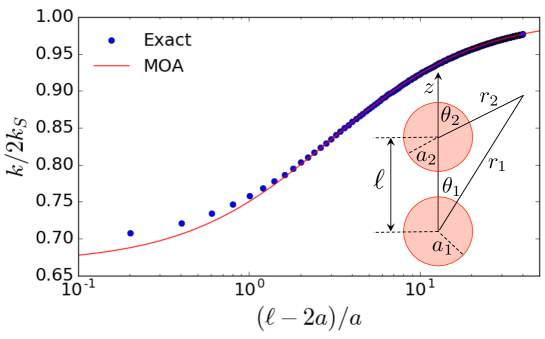
Figure 1: Rate of capture for two sinks of radius $a_{1}=a_{2}=a$ separated by a distance $\ell$. Comparison of the exact result and the MOA approximation.

It can be appreciated that $k\to 2k_{S}$ in the limit of infinite separation, $\ell\to\infty$. The MOA predicts a maximum reduction $k/2k_{S}=2/3$ of the rate of capture (i.e. maximum strength of DIs) at contact distance, $\ell=2a$. This has to be compared with the exact value [64], $k/2k_{S}=\log 2\approx 0.693$. It is interesting to observe that DIs are long-range, that is $1-k/2k_{S}\simeq a/\ell$ for separations larger than a few radii: DIs are entropic forces that decay with distance like Coulomb and gravitational interactions.
One may wonder how good an approximation is the MOA. It turns out that for assemblies of perfectly absorbing sinks it is indeed an extremely good approximation, as it is apparent from f:twosinksMOA. For $\ell=3a$ the relative error is less than 1 %. It can be shown that the relative error decreases rapidly, $\propto\ell^{-4}$, until $\ell\simeq 10a$ (approximately 0.01 %), and then decreases more slowly, $\propto\ell^{-1}$. The reasons why the MOA is so good an approximation have been investigated in Ref. 18.

2 Diffusive interactions are weaker among multiple partially reactive boundaries

A system of partially reactive boundaries experiences weaker diffusive interactions. This can be easily seen and quantified by repeating the above calculations for two spheres endowed with intrinsic rate constants $\kappa_{1}$ and $\kappa_{2}$. This entails replacing boundary conditions (14b) with radiation conditions, namely

$$\left[\frac{\partial u}{\partial\xi_{i}}-h_{i}(u-1)\right]_{\xi_{i}=1}=0$$ (25)

where $h_{i}=\kappa_{i}^{\ast}/\kappa_{S_{i}}$, $i=1,2$. In this case, it is not difficult to take the same steps as in the above derivation and compute the new matrices $U^{12}$, $U^{21}$. The MOA gives in this case

$$k=k_{S_{1}}\left[\frac{q_{1}(1-q_{2}\epsilon_{2})}{1-q_{1}q_{2}\epsilon_{1}\epsilon_{2}}\right]+k_{S_{2}}\left[\frac{q_{2}(1-q_{1}\epsilon_{1})}{1-q_{1}q_{2}\epsilon_{1}\epsilon_{2}}\right]$$ (26)

where $q_{i}=h_{i}/(1+h_{i})$. The case of two identical, partially absorbing spheres gives immediately

$$\frac{k}{2k_{S}}=\frac{h}{1+h(1+\epsilon)}\leq\frac{1}{1+\epsilon}$$ (27)

Diffusive interactions are therefore less prominent for partially absorbing boundaries. It is easy to check that the maximum strength of DIs (i.e. at contact distance) is reduced by an intrinsic reaction rate $\kappa^{\ast}$ by a factor $3h/(2+3h)$ in the MOA. However, it should be emphasized that the MOA performs increasingly worse the lower the value of $h$, and more multipoles should be considered beyond the $n=0$ term to achieve the same accuracy as in the limit $h\to\infty$.

5 Many spherical boundaries arranged arbitrarily in space

The trick of using addition theorems to express multipole expansions in local reference frames centered on two different disconnected spherical boundaries can be extended with no conceptual difficulties to the case of many spheres of arbitrary size, intrinsic reaction rate constant and position in 3D space. Let us consider the finite spherical domain $\displaystyle\Omega=\Omega_{0}\setminus\bigcup_{\alpha=1}^{N}\overline{\Omega}_{\alpha}$, represented in f:schemacoord, filled with $N$ spherical reactive boundaries. Let us introduce the non-dimensional normalized ligand density $u(\mathbb{r})=c(\mathbb{r})/c_{B}$ and the variables $\xi_{\alpha}=r_{\alpha}/R_{\alpha}$, $\xi_{0}=r_{0}/R_{0}$, normalized to the radii of the respective reactive boundaries. We need to solve the following boundary problem

$$\displaystyle\bigtriangledown^{2}u=0$$ (28a)

$$\displaystyle\bigg{(}\left.\frac{\partial u}{\partial\mathbb{\xi_{\alpha}}}-h_{\alpha}u\bigg{)}\right|_{\partial\Omega_{\alpha}}=0\qquad\forall\,\alpha=1,2,\dots,N$$ (28b)

$$\displaystyle\left.\bigg{(}\frac{\partial u}{\partial{\xi_{0}}}+h_{0}(u-1)\bigg{)}\right|_{\partial\Omega_{0}}=0$$ (28c)

Again, we have introduced the parameters $h_{\alpha}={\kappa_{\alpha}^{\ast}}/{4\pi DR_{\alpha}}$ that determine the reactivity of the $\alpha$-th sphere. The boundary condition (28c) on the inner surface of the container sphere $\Omega_{0}$ is a radiation-type boundary condition and has the following meaning. One should imagine that the ligand concentration is $c_{B}$ outside $\Omega_{0}$ (even if formally the problem is not defined there) and that there is a membrane separating the inner compartment $\Omega$ from the exterior whose non-dimensional permeability is proportional to $h_{0}$. In the limit $R_{0}\to\infty$, one recovers the open-boundary problem with the boundary condition $\lim_{R_{0}\to\infty}c=c_{B}$. Furthermore, it is not difficult to show that if one considers the problem (28) for a single sink at the center of $\Omega_{0}$ and an equivalent problem (single sink) in the open domain but with $D=\{D_{\rm in}\ \text{for}\ r\leq R_{0}|\ D_{\rm out}\ \text{for}\ r>R_{0}\}$, then the two problems are equivalent provided $h_{0}=D_{\rm out}/D_{\rm in}$. Hence, one may think of the problem (28) as describing diffusion of ligand to a set of spheres within a spherical container such that the ligand concentration outside the container is fixed ($c_{B}$), as well as the ratio $h_{0}$ between the ligand diffusion coefficient outside the container (bulk) and in the interior, the latter parameter playing the role of the non-dimensional permeability of the (imaginary) membrane at $\partial\Omega_{0}$.
By virtue of the superposition principle for the Laplace equation, the problem (28) admits a solution in $\Omega$ as a sum of linear combinations of regular (inside $\Omega_{0}$) and irregular harmonics (outside each $\Omega_{\alpha}$), namely

$$u = u^{+}_{0}+\sum_{\alpha=1}^{N}u^{-}_{\alpha}$$ (29)

$$= \sum_{n=0}^{\infty}\sum_{m=-n}^{n}A_{mn}\xi_{0}^{n}Y_{mn}(\boldsymbol{r}_{0})+\sum_{\alpha=1}^{N}\sum_{n=0}^{\infty}\sum_{m=-n}^{n}B_{mn}^{\alpha}\xi_{\alpha}^{-n-1}Y_{mn}(\boldsymbol{r}_{\alpha})$$

where $Y_{mn}(\boldsymbol{r}_{\alpha})=P^{m}_{n}(\cos\theta_{\alpha})e^{im\phi_{\alpha}}$ are solid harmonics referring to the local reference frame centered on the $\alpha$-th boundary (see f:schemacoord). The coefficients $A_{mn},B^{\alpha}_{mn}$ should be determined by imposing the boundary conditions. In the neighborhood of each boundary one has to express all the bases as a function of the local coordinates. More precisely, in the neighborhood of each $\partial\Omega_{\alpha}$, $u^{+}_{0}$ and $u^{-}_{\beta}$ ($\beta\neq\alpha$) have to be expressed as a function of the $\boldsymbol{r}_{\alpha}$ coordinates, and similarly, in the neighborhood of $\partial\Omega_{0}$, every $u^{-}_{\alpha}$ has to be written as a function of $\boldsymbol{r}_{0}$. For this purpose, one can make use of the translational addition theorems (AT) for solid harmonics [47]. This operation requires some care, as one out of three possible ATs must be selected for each pair of boundaries depending on the geometry. These rules are summarized in appendix  ‣ Acknowledgements.

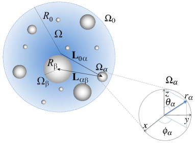
Figure 2: Schematic representation of the domain $\Omega$ with the relevant local coordinate systems, radii and position vectors.

1 Many spheres inside a spherical cavity

Diffusion-influenced reactions inside a spherical cavity are of great importance in various applications, however, often the simple Smoluchowski rate is incorrectly used to describe the kinetics of these reactions [66, 67].
The rate of capture of a sink of radius $R_{1}$ at the center of a spherical cavity of radius $R_{0}$ outside which there is a constant bulk ligand density $c_{B}$ is given by the solution of the following problem

$$\displaystyle\bigtriangledown^{2}u=0$$ (30a)

$$u|_{r=R_{1}}=0$$ (30b)

$$\left.\bigg{(}R_{0}\frac{\partial u}{\partial r}+h_{0}(u-1)\bigg{)}\right|_{r=R_{0}}=0$$ (30c)

where $u(r)=c(r)/c_{B}$ and $h_{0}=D_{\rm out}/D_{\rm in}$ is a parameter gauging the permeability of the internal boundary of the spherical cavity. Here we assume that $D_{\rm out},D_{\rm in}$ are the ligand diffusion coefficient outside and inside the cavity, respectively. The solution to the problem (30) is straightforward, and the capture rate by (total flux into) the sink yields

$$\frac{k}{k_{S_{1}}}=\frac{h_{0}}{\epsilon+h_{0}(1-\epsilon)}$$ (31)

where $\epsilon=R_{1}/R_{0}$. We see that $k\to k_{S_{1}}=4\pi D_{\rm in}c_{B}$ in the limit of infinite cavity $R_{0}\to\infty$. For a finite cavity with a fixed ligand concentration outside, e:1sinkcavk has a simple interpretation: the rate of capture is enhanced for $h_{0}>1$, that is, when $D_{\rm out}>D_{\rm in}$. In the limit of infinitely absorbing boundary (or conversely, infinitely viscous interior), the rate of capture is enhanced by a factor $1/(1-\epsilon)$. This becomes very large as the sink approaches the inner surface of the cavity.
This simple result may have interesting implications for the diffusion of ligands within the bacterial periplasm. This region, comprised between the outer cell membrane and an inner (cytoplasmic) membrane, can be as wide as 40 % of the total volume in gram-negative bacteria and is typically a very shallow layer in gram-positive bacteria. The periplasm is filled with a thick gel-like, highly crowded matrix [68] and is lined up with many arrays of receptors on the inner cytoplasmic membrane, facing the outer membrane (interior of the cavity). Many ligands, such as those related to chemotaxis, diffuse to receptors within the inner membrane (at $r=R_{1}$). Since typically $(R_{0}-R_{1})/R_{0}\ll 1$ and the periplasm is very crowded [68], one has $D_{\rm in}\ll D_{\rm out}$ and $1-\epsilon\ll 1$, which would thence boost the rate of capture.
Using the general addition theorems for solid harmonics (see details reported in appendix  ‣ Acknowledgements), we are now in a position to answer many interesting questions related to such problems.

Two spheres inside a spherical cavity

It is interesting to investigate diffusion interactions between two sinks in a finite domain. Let us consider the simple case of two identical perfect sinks arranged symmetrically along a diameter of a spherical cavity with respect to the center. Let us denote with $\ell$ the center-center distance, with $R_{1}$ the size of the sinks and with $R_{0}$ the size of the cavity, whose internal surface is made perfectly absorbing. The problem (28) can be solved as described in appendix  ‣ Acknowledgements. The results are summarized in f:2sphcav. In agreement with what discussed in the previous section, one can appreciate that the rate to the two confined sinks is larger than in the absence of cavity. In particular the rate increases abruptly as the sinks approach the inner boundary of the cavity. This is a direct consequence of the assumption that the ligand density at the cavity interface is equal to the bulk density. Another non-trivial observation is that the normalized rate now depends on the size of the sink: large sinks have more capture power with respect to the open-domain, non-confined setting than small ones. Concerning the rate of capture of single confined sinks, one remarks that the prediction (31) in the limit $h_{0}\to\infty$ for a sink at the center of the cavity is still accurate when the sink is displaced up to a distance of $\simeq 7\div 8R_{1}$ from the center (constant curves with squares in f:2sphcav, left panel).
The rates increase in a cavity and diffusive interactions decrease. This effect is illustrated in the right panel of f:2sphcav. The larger the embedded sinks, the greater the overall rate and correspondingly the weaker the diffusive interactions. For example, for $R_{1}/R_{0}=0.2$, the DIs are practically gone ($k_{2}=2k_{1}$) already for $\ell\simeq 5\div 6R_{1}$, i.e. when the outer surface of the sinks is at a distance of about $0.2R_{0}$ from the inner surface of the cavity.

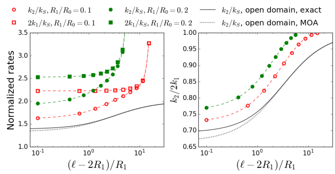
Figure 3: Rate of capture by two identical spheres of radius $R_{1}$ inside a spherical cavity of radius $R_{0}$ with absorbing inner boundary ($h_{0}\to\infty$). With reference to a frame with the origin at the center of $\Omega_{0}$, the two spheres are placed symmetrically along the $z$ axis at a center-center separation $\ell\in[2R_{1},2(R_{0}-R_{1})]$. Left: normalized rates of the two-sphere system compared with twice the rate of one isolated sink at the same position vs rescaled center-center distance. The rates are normalized to the rate of one isolated sink in the open domain, $k_{S}=4\pi DR_{1}c_{B}$. Right: measure of diffusive interactions. The caption refers to the left panel. Symbols and lines in the right panel refer to the same cases as in the left panel.

Many sinks on a spherical inner layer inside a spherical cavity

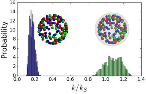
Figure 4: Histograms of the individual capture rate of $N=50$ identical sinks of radius $R_{1}=R_{0}/10$ arranged at a fixed distance $d=0.95\times(R_{0}-R_{1})$ from the center of a spherical cavity with absorbing inner wall (right) and in the infinite domain (left). The histograms are normalized to the capture rate of an isolated sink in the open domain, $k_{S}=4\pi DR_{1}c_{B}$. The histograms refer to a population of 100 independent random configurations of the $N=50$ sinks, 3 of which are pictured explicitly to illustrate the geometry of the problem.

It is instructive to use the above described method to investigate the rate of capture of many equivalent sinks arranged randomly at a given distance from the center on a spherical layer. In the open domain, the rate to such ensembles of sinks is strongly reduced due to diffusive interactions. For example, the average capture rate of random configurations of $N=50$ non-overlapping sinks of size $R_{1}$ at a distance $d=8.85R_{1}$ from the center is $k_{50}=(8.33\pm 0.01)k_{S}$, with $k_{S}=4\pi DR_{1}c_{B}$ (average over 100 independent configurations). DIs reduce by a staggering 85 % the overall capture rate of the ensemble with respect to as many isolated sinks. We have learned that confining sinks within a cavity helps sustain the capture rate due to the proximity (exterior of the cavity) of the bulk concentration (effectively reducing the ligand depletion region). In fact, the same ensembles of sinks within a cavity of radius $R_{0}=10R_{1}$, i.e. close to the inner surface of the cavity, display a rate of capture $k^{\rm c}_{50}=(54.2\pm 0.2)k_{S}$. This corresponds to a situation of even positive cooperativity. This situation is found for example in the bacterial periplasm. It is reasonable to assume that ligands, whose concentration is constant outside the cell, diffuse very slowly in the periplasm as compared to the bulk, which justifies the assumption $h_{0}\gg 1$. It is fascinating to think that such a complex, double-membrane architecture could be a an evolutive answer to the requirement of maximizing the diffusive flux of (possibly low-concentration) ligands to a set of membrane-bound receptors.
f:3confallk reveals what happens to the individual capture rates for a large set of equivalent configurations of receptors on the inner membrane of an imaginary periplasmatic layer. Each receptor-sink is seen to capture on average the same amount of flux it would capture if it was isolated at the center of the cavity (see e:1sinkcavk for $h_{0}\to\infty$), i.e. about $1/(1-R_{1}/R_{0})\approx 1.11$ in units of $k_{S}$. This somewhat surprising fact is due to the close proximity of the sinks to the inner surface of the cavity (see also again f:2sphcav). If the cavity disappears, this figure drops down to about $0.15\,k_{S}$ (left histogram in f:3confallk). This is another manifestation of the virtual suppression of diffusive interactions for sinks close to the absorbing inner surface of a cavity. Furthermore, it can be observed that the intrinsic variability of the capture rate around the ensemble average is reduced when diffusive interactions are strong (width of the left histogram in f:3confallk). This means that when DIs are weaker, not only the ensemble recovers a large rate of capture on average, but some of the receptors-sink individually can attain large peaks of capture rate.

6 Summary

In this short, mostly pedagogical review, we have described the phenomenon of diffusion to capture, which has important implications in a wide range of fields in biology and physical chemistry. We have shown how, under certain circumstances, the problem of bimolecular encounters and reactions can be solved as a two-body stationary diffusion boundary problem. This theoretical framework immediately leads to some surprising conclusions. One of the most striking findings concerns the rate of ligand capture by a receptor-covered cell. The classic mean-field solution of this problem shows that a fraction of surface coverage as low as $10^{-4}$ (approximately $10^{4}$ receptors of $1.5$ nm size on the surface of a cell of size $10$ $\mu$m) ensures that the overall rate of capture is of the same order (reduced by a factor of 2) as for a fully covered surface. Moreover, we have shown that if the same number of active receptors are all moved into an active cluster covering the same surface fraction, the overall rate of capture drops by a factor of up to $10^{2}$. This is a first manifestation of diffusive interactions, which describe the interference among diffusive fluxes to neighboring reactive boundaries.
In order to provide a rigorous mathematical description of diffusive interactions, we have considered in detail the classic problem of diffusion to two neighboring sinks at a center-to-center distance $\ell$ in the open domain. Although this problem can be solved by using bispherical coordinates [64], we have followed another, more general approach, based on translational addition theorems for spherical harmonics [47]. The exact solution of the problem, expressed in the form of an infinite series of multipoles, can be surprisingly well approximated for perfectly absorbing spheres by the monopole term alone, showing that diffusive interactions are long-range, i.e. decrease as $\ell^{-1}$.
The mathematical strategy based on addition theorems can be easily extended to compute the rate of capture of an ensemble of spheres of arbitrary, size, intrinsic reactivity ($\kappa^{\ast}$) and arranged in arbitrary configurations in 3D, both in the open domain and within a spherical cavity. This theory, developed in Ref. 46, is described in detail in appendix  ‣ Acknowledgements. Although the applications of such theoretical framework are countless, we have examined here two simple examples. First we have studied the case of two sinks within a cavity, whose solution shows that diffusive interactions are generally reduced in a finite domain with an absorbing inner surface, concomitantly with the enhancement of the rate of capture. This phenomenon is due to the fact that, in this modeling strategy, the density of ligands reaches its constant bulk value outside the cavity (whose surface is modeled as a permeable membrane), which enhances the rate of capture of a given boundary with respect to the open domain. Interestingly, now the relative position of the boundary within the cavity obviously makes a difference, the rate of capture increasing massively as the boundary approaches the inner surface of the cavity. At the same time, if many sinks are present, the diffusive interactions among them are virtually suppressed for many-body configurations close to the inner surface of the cavity. The second and final example studied, namely many independent configurations of sinks close to the inner surface of the cavity, shows this clearly. Finally, we have argued that this problem, while interesting on purely theoretical grounds, might also have important implications in ligand-receptor interactions in biology. Notably, ligand diffusion to receptors on the cytoplasmatic membrane in the periplasmatic space in bacteria provides an example of this problem. In this specific case, ligand diffusion in the crowded, gel-like periplasm is likely to be strongly reduced with respect to the mobility in the bulk outside, which justifies modeling the inner surface of the outer (cell) membrane as an absorbing boundary. The fascinating speculation that follows from these results is that such a complex architecture might have been designed by evolution to maximize the ligand-receptor binding rate. This would make sense, as such receptors are mostly chemotaxis receptors, used by bacteria to sense gradients of nutrients (small molecules).

Acknowledgements

This work was partially supported within the framework of the state task program of the FASO Russia (Theme 0082-2014-008, No AAAA-A17-117040310008-5).

[Rules for selecting the appropriate addition theorem]

The addition theorems for spherical harmonics allow one to express a combination of spherical harmonics, written in multiple coordinate systems, as a function of any one of them. Depending on the type of spherical harmonic that one needs to re-expand (regular or irregular) and on the geometry of the domain, one among three addition theorems has to be chosen in each specific case. Let us suppose to have spherical harmonics $u^{+}(\boldsymbol{r}_{\beta})$ and $u^{-}(\boldsymbol{r}_{\beta})$ written in a spherical coordinate system centered on $S_{\beta}$, that we want to express at a given point $P$ as a function of the $S_{\alpha}$-coordinate system (see f:schemacoord). The relation $\boldsymbol{r}_{\beta}=\mathbb{L}_{\beta\alpha}+\mathbb{r}_{\alpha}$ holds. The regular harmonics $u^{+}(\mathbb{r}_{\beta})$ are always expressed as a function of the regular harmonics $u^{+}(\mathbb{r}_{\alpha})$, namely

$$\begin{split}&r_{\beta}^{n}Y_{mn}(\mathbb{r}_{\beta})=\\ &\sum_{q=0}^{n}\sum_{g=-q}^{q}\frac{(n+m)!}{(n-q+m-g)!(q+g)!}L_{\beta\alpha}^{n-q}Y_{m-g,n-q}(\boldsymbol{L}_{\beta\alpha})r_{\alpha}^{q}Y_{gq}(\boldsymbol{r}_{\alpha}).\end{split}$$ (32)

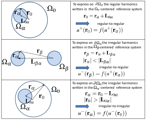
Figure 5: Scheme for the the application of the addition theorems (32), (33) and  (34) to express the boundary conditions in the local coordinates on $\partial\Omega_{0}$ and on each $\partial\Omega_{\alpha}$. The choice of the appropriate addition theorem depends on the ratio between the distance between the centers of each pair of reference systems and the norm of the position vector in the new reference system.

If one has to re-expand an irregular harmonic $u^{-}(\boldsymbol{r}_{\beta})$, two cases are possible, depending on the ratio between the distance $L_{\beta\alpha}$ between the centers of the old and new reference frames, and the norm of the the vector $\boldsymbol{r}_{\alpha}$ expressing the position of $P$ in the new frame $S_{\alpha}$ . More precisely, if $|\boldsymbol{r}_{\alpha}|<|\boldsymbol{L}_{\beta\alpha}|$, then one has to write the irregular harmonic as a function of the regular harmonics centered on $S_{\alpha}$, namely

$$\begin{split}&\small r_{\beta}^{-n-1}Y_{mn}(\boldsymbol{r_{\beta}})=\\ &\sum_{q=0}^{\infty}\sum_{g=-q}^{q}(-1)^{q+g}\frac{(n-m+q+g)!}{(n-m)!(q+g)!}L_{\beta\alpha}^{-(n+q)-1}Y_{m-g,n+q}(\boldsymbol{L}_{\beta\alpha})r_{\alpha}^{q}Y_{gq}(\boldsymbol{r}_{\alpha}).\end{split}$$ (33)

Conversely, if $|\boldsymbol{r}_{\alpha}|>|\boldsymbol{L}_{\beta\alpha}|$, then one has to write the irregular harmonic as a function of the irregular harmonics centered in $S_{\alpha}$:

$$\begin{split}&r_{\beta}^{-n-1}Y_{mn}(\boldsymbol{r_{\beta}})=\\ &\sum_{l=0}^{\infty}\sum_{s=-n}^{n}\frac{(-1)^{l+s}(n+l-m+s)!}{(n-m)!(l+s)!}L_{\alpha\beta}^{l}Y_{sl}(-\boldsymbol{L}_{\alpha\beta})r_{\alpha}^{-(n+l)-1}Y_{m-s,n+l}(\boldsymbol{r_{\alpha}}).\end{split}$$ (34)

To summarize, one can use the following scheme to change variables from system $S_{\beta}$ to $S_{\alpha}$ (see also addi)

• $u^{+}(\boldsymbol{r}_{\beta})=f(u^{+}(\boldsymbol{r}_{\alpha}))$

• $u^{-}(\boldsymbol{r}_{\beta})=\begin{cases}f(u^{+}(\boldsymbol{r}_{\alpha}))\quad\text{if}\quad|\boldsymbol{r}_{\alpha}|<|\mathbb{L}_{\beta\alpha}|\\ f(u^{-}(\boldsymbol{r}_{\alpha}))\quad\text{if}\quad|\boldsymbol{r}_{\alpha}|>|\mathbb{L}_{\beta\alpha}|\end{cases}$.

1 The solution to the problem

By using the above addition theorems, the solution to the problem (28) can be cast in the form of the following infinite-dimensional linear system,

$$\begin{cases}\displaystyle-B_{gq}^{\alpha}+\sum_{n=0}^{\infty}\sum_{m=-n}^{n}\bigg{(}A_{mn}H_{m,n}^{(\alpha,g,q)}\mathbf{1}_{q\leq n}+\sum_{\beta=1,\beta\neq\alpha}^{N}B_{mn}^{\beta}W_{m,n}^{(\alpha,\beta,g,q)}\bigg{)}=0\\ \displaystyle A_{gq}+\sum_{\alpha=1}^{N}\sum_{n=0}^{q}\sum_{m=-n}^{n}B_{mn}^{\alpha}V_{g,q}^{\alpha,m,n}\mathbf{1}_{\{g-(q-n)\leq m\leq g+(q-n)\}}=\delta_{(g,q)=(0,0)}.\\ \end{cases}$$ (35)

where

$$\begin{split}V_{g,q}^{\alpha,m,n}=-\frac{h_{0}+q+1}{(q-h_{0})}\frac{(-1)^{q-n+m-g}(q-g)!}{(n-m)!(q-n+m-g)!}\eta_{0\alpha}^{q-n}\chi_{\alpha}^{n+1}Y_{m-g,q-n}(-\boldsymbol{L_{0\alpha}})\end{split}$$ (36)

$$H_{m,n}^{(\alpha,g,q)}=\frac{(q-h_{\alpha})}{(h_{\alpha}+q+1)}\binom{n+m}{q+g}\chi_{\alpha}^{q}\eta_{0\alpha}^{n-q}Y_{m-g,n-q}(\boldsymbol{L_{0\alpha}})$$ (37)

$$\begin{split}W_{m,n}^{(\alpha,\beta,g,q)}=\frac{(q-h_{\alpha})}{(h_{\alpha}+q+1)}&(-1)^{q+g}\times\\ &\frac{(n-m+q+g)!}{(n-m)!(q+g)!}\eta_{\beta\alpha}^{-(n+q)-1}\chi_{\alpha}^{q}\chi_{\beta}^{n+1}Y_{m-g,n+q}(\boldsymbol{L_{\beta\alpha}})\end{split}$$ (38)

with $\displaystyle\chi_{\alpha}:=\frac{R_{\alpha}}{R_{0}}$ and $\displaystyle\eta_{\alpha\beta}:=\frac{L_{\alpha\beta}}{R_{0}}$ with $\eta_{\alpha\beta}=\eta_{\beta\alpha}$. The system (35) can be cast in matrix form as follows:

$$\left[\vbox{\hbox{\hbox to0.0pt{\hbox{\kern 0.0pt\hbox{\vbox{\vbox{}\hrule width=0.0pt,height=0.0pt,depth=0.0pt}\kern 0.0pt\hbox{\kern 0.0pt\hbox{\kern 0.0pt\hbox{\kern 0.0pt\hbox{}}}}}}\hss}\hbox to0.0pt{\vbox{\kern 0.0pt\vbox{\hbox{\hbox{}\vrule width=0.0pt,height=0.0pt,depth=0.0pt}\kern 0.0pt\vbox{\kern 0.0pt\vbox{}}}}\hss}\vbox{\kern 0.0pt}}}\right]\times\left[\vbox{\hbox{\hbox to0.0pt{\hbox{\kern 0.0pt\hbox{}}\hss}\hbox to0.0pt{\vbox{\kern 0.0pt\vbox{\kern 0.0pt\vbox{\kern 0.0pt\vbox{\hbox{\hbox{}\vrule width=0.0pt,height=0.0pt,depth=0.0pt}\kern 0.0pt\vbox{\kern 0.0pt\vbox{\kern 0.0pt\vbox{\hbox{\hbox{}\vrule width=0.0pt,height=0.0pt,depth=0.0pt}\kern 0.0pt\vbox{\hbox{\hbox{}\vrule width=0.0pt,height=0.0pt,depth=0.0pt}\kern 0.0pt\vbox{}}}}}}}}}\hss}\vbox{\kern 0.0pt}}}\right]=\left[\vbox{\hbox{\hbox to0.0pt{\hbox{\kern 0.0pt\hbox{}}\hss}\hbox to0.0pt{\vbox{\kern 0.0pt\vbox{\kern 0.0pt\vbox{\kern 0.0pt\vbox{\hbox{\hbox{}\vrule width=0.0pt,height=0.0pt,depth=0.0pt}\kern 0.0pt\vbox{\kern 0.0pt\vbox{\kern 0.0pt\vbox{\hbox{\hbox{}\vrule width=0.0pt,height=0.0pt,depth=0.0pt}\kern 0.0pt\vbox{\hbox{\hbox{}\vrule width=0.0pt,height=0.0pt,depth=0.0pt}\kern 0.0pt\vbox{}}}}}}}}}\hss}\vbox{\kern 0.0pt}}}\right]$$

2 The rate

The capture rate for a ligand with diffusion coefficient $D$ by a selected boundary $\Omega_{\alpha}$ can be computed easily as the total incoming flux, namely

$$k_{\alpha}=-\int_{\partial\Omega_{\alpha}}\boldsymbol{J}_{\alpha}\cdot\hat{\boldsymbol{n}}\,dS$$ (39)

where $\boldsymbol{J}_{\alpha}=-D\nabla_{\alpha}c$ is the current to the $\alpha$-th boundary. It is not difficult to see from the general form of the solution (29) and general properties of the Legendre polynomials $P^{m}_{n}(\mu_{\alpha})$ that e:rate_alpha_def gives

$$\frac{k_{\alpha}}{k_{S_{\alpha}}}=-B_{00}^{\alpha}$$ (40)

where $k_{S_{\alpha}}=4\pi DR_{\alpha}c_{B}$ is the Smoluchowski rate of capture corresponding to an isolated sink of radius $R_{\alpha}$ in the infinite domain.

References

- 1. S. Rice, Diffusion-Limited Reactions. Elsevier, Amsterdam (1985).
- 2. F. Piazza, G. Foffi, and C. De Michele, Irreversible bimolecular reactions with inertia: from the trapping to the target setting at finite densities, Journal of Physics: Condensed Matter. 25(24), 245101 (2013).
- 3. S. Torquato, Random Heterogenous Materials. Interdisciplinary Applied Mathematics, Springer-Verlag, New York (2002).
- 4. J. Crank, The mathematics of diffusion. Oxford science publications (1975).
- 5. M. Labowsky and T. M. Fahmy, Diffusive transfer between two intensely interacting cells with limited surface kinetics, Chemical Engineering Science. 74, 114–123 (2012).
- 6. H. X. Zhou, G. Rivas, and A. P. Minton, Macromolecular crowding and confinement: biochemical, biophysical, and potential physiological consequences, Annual review of biophysics. 37, 375–397 (2008).
- 7. A. S. Verkman, Solute and macromolecule diffusion in cellular aqueous compartments., Trends in biochemical sciences. 27(1), 27–33 (Jan., 2002).
- 8. K. Luby-Phelps, Cytoarchitecture and physical properties of cytoplasm: volume, viscosity, diffusion, intracellular surface area., International review of cytology. 192, 189–221 (2000).
- 9. A. M. Berezhkovskii and A. Szabo, Theory of Crowding Effects on Bimolecular Reaction Rates., The journal of physical chemistry. B (may, 2016).
- 10. S. D. Traytak, Ligand binding in a spherical region randomly crowded by receptors., Physical biology. 10(4), 045009 (2013).
- 11. F. Piazza, N. Dorsaz, C. De Michele, P. De Los Rios, and G. Foffi, Diffusion-limited reactions in crowded environments: a local density approximation, Journal of Physics: Condensed Matter. 25(37), 375104 (2013).
- 12. N. Dorsaz, C. De Michele, F. Piazza, P. De Los Rios, and G. Foffi, Diffusion-Limited Reactions in Crowded Environments, Physical Review Letters. 105(12), 120601 (sep, 2010).
- 13. C. Echevería, K. Tucci, and R. Kapral, Diffusion and reaction in crowded environments, Journal of Physics: Condensed Matter. 19(6), 065146 (2007).
- 14. H. L. Frisch and F. C. Collins, Diffusional processes in the growth of aerosol particles. II, The Journal of Chemical Physics. 21(12), 2158–2165 (1953).
- 15. R. A. Reck and S. Prager, Diffusion-controlled quenching at higher quencher concentrations, The Journal of Chemical Physics. 42(9), 3027–3032 (1965).
- 16. V. A. Borzilov and A. S. Stepanov, On the derivation of the equation for condensation of an array of drops, Izv. Atmos. Ocean. Phys. 7, 164–172 (1971).
- 17. J. M. Deutch, B. U. Felderhof, and M. J. Saxton, Competitive effects in diffusion-controlled reactions, J. Chem. Phys. 64, 4559 (1976).
- 18. S. Traytak, The diffusive interaction in diffusion-limited reactions: the steady-state case, Chemical Physics Letters. 197, 247–254 (9, 1992).
- 19. H. C. Berg, Random walks in biology. Princeton University Press (1993).
- 20. V. Sourjik, Receptor clustering and signal processing in E. coli chemotaxis., Trends in microbiology. 12(12), 569–76 (dec, 2004).
- 21. J.-D. Lelièvre, F. Petit, L. Perrin, F. Mammano, D. Arnoult, J.-C. Ameisen, J. Corbeil, A. Gervaix, and J. Estaquier, The Density of Coreceptors at the Surface of CD4+ T Cells Contributes to the Extent of Human Immunodeficiency Virus Type 1 Viral Replication-Mediated T Cell Death, AIDS Research and Human Retroviruses. 20(11), 1230–1243 (nov, 2004).
- 22. C. DeLisi and F. W. Wiegel, Effect of nonspecific forces and finite receptor number on rate constants of ligand-cell bound-receptor interactions., Proceedings of the National Academy of Sciences of the United States of America. 78(9), 5569–5572 (1981).
- 23. A. Briegel, D. R. Ortega, E. I. Tocheva, K. Wuichet, Z. Li, S. Chen, A. Müller, C. V. Iancu, G. E. Murphy, M. J. Dobro, I. B. Zhulin, and G. J. Jensen, Universal architecture of bacterial chemoreceptor arrays., Proceedings of the National Academy of Sciences of the United States of America. 106(40), 17181–6 (oct, 2009).
- 24. Š. Bálint, M. L. Dustin, A. Bruckbauer, F. Batista, S. Banjade, J. Okrut, D. King, J. Taunton, M. Rosen, R. Vale, Z. Guo, R. Vishwakarma, M. Rao, S. Mayor, D. Klenerman, A. Aricescu, and S. Davis, Localizing order to boost signaling, eLife. 6, 1055–1068 (mar, 2017).
- 25. S. Angioletti-Uberti, Exploiting Receptor Competition to Enhance Nanoparticle Binding Selectivity, Physical Review Letters. 118(6) (2017).
- 26. W. S. Hlavacek, R. G. Posner, and A. S. Perelson, Steriuc effects on multivalent ligand-receptor binding: Exclusion of ligand sites by bound cell surface receptors, Biophysical Journal. 76, 3031–3043 (1999).
- 27. G. Vauquelin and S. J. Charlton, Exploring avidity: understanding the potential gains in functional affinity and target residence time of bivalent and heterobivalent ligands, British Journal of Pharmacology. 168(8), 1771–1785 (apr, 2013).
- 28. A. Todorovska, R. C. Roovers, O. Dolezal, A. A. Kortt, H. R. Hoogenboom, and P. J. Hudson, Design and application of diabodies, triabodies and tetrabodies for cancer targeting, Journal of Immunological Methods. 248(1-2), 47–66 (feb, 2001).
- 29. N. Nuñez-Prado, M. Compte, S. Harwood, A. Álvarez-Méndez, S. Lykkemark, L. Sanz, and L. Álvarez-Vallina, The coming of age of engineered multivalent antibodies, Drug Discovery Today. 20(5), 588–594 (2015).
- 30. C. Fasting, C. A. Schalley, M. Weber, O. Seitz, S. Hecht, B. Koksch, J. Dernedde, C. Graf, E.-W. Knapp, and R. Haag, Multivalency as a Chemical Organization and Action Principle, Angewandte Chemie International Edition. 51(42), 10472–10498 (oct, 2012).
- 31. M. Mammen, S.-K. Choi, and G. M. Whitesides, Polyvalent interactions in biological systems: Implications for design and use of multivalent ligands and inhibitors, Angewandte Chemie International Edition. 37(20), 2754–2794 (1998).
- 32. I. V. Gopich, A. M. Berezhkovskii, and A. Szabo, Concentration dependence of the diffusion controlled steady-state rate constant, Journal of Chemical Physics. 117, 2987–2988 (2002).
- 33. A. M. Berezhkovskii, D. J. Bicout, and G. H. Weiss, Target and trapping problems: From the ballistic to the diffusive regime, The Journal of Chemical Physics. 110, 1112 (1999).
- 34. S. Yuste, G. Oshanin, K. Lindenberg, O. Bénichou, and J. Klafter, Survival probability of a particle in a sea of mobile traps: A tale of tails, Physical Review E. 78(2), 021105 (aug, 2008).
- 35. S. D. Traytak and M. Tachiya, Concentration dependence of fluorescence quenching by ionic reactants, Journal of Physics: Condensed Matter. 19(6), 065111 (2007).
- 36. J. Keizer, Diffusion effects on rapid bimolecular chemical reactions, Chemical Reviews. 87(1), 167–180 (02, 1987).
- 37. B. U. Felderhof and J. M. Deutch, Concentration dependence of the rate of diffusion-controlled reactions, Journal of Chemical Physics. 64(11), 4551–4558 (june, 1976).
- 38. M. Galanti, D. Fanelli, S. Angioletti-Uberti, M. Ballauff, J. Dzubiella, and F. Piazza, Reaction rate of a composite core-shell nanoreactor with multiple nanocatalysts, Physical Chemistry Chemical Physics. 18(30), 20758–20767 (2016).
- 39. F. Piazza and S. D. Traytak, Diffusion-influenced reactions in a hollow nano-reactor with a circular hole, Phys. Chem. Chem. Phys. 17(16), 10417–10425 (2015).
- 40. Y. Lu and M. Ballauff, Thermosensitive core–shell microgels: From colloidal model systems to nanoreactors, Progress in Polymer Science. 36(6), 767–792 (jun, 2011).
- 41. A. Sozza, F. Piazza, M. Cencini, F. De Lillo, and G. Boffetta, Point-particle method to compute diffusion-limited cellular uptake, Physical Review E. 97(2) (2018).
- 42. S. D. Traytak, The diffusive interaction in diffusion-limited reactions: the time-dependent case, Chemical Physics. 193, 351–366 (1995).
- 43. S. D. Traytak, On the time-dependent diffusive interaction between stationary sinks, Chemical Physics Letters. 453, 212–216 (2008).
- 44. S. D. Traytak, Competition effects in steady-state diffusion-limited reactions: Renormalization group approach, Journal of Chemical Physics. 105(24), 10860–10867 (1996).
- 45. E. Gordelyi, S. Crouch, and S. Mogilevskaya, Transient heat conduction in a medium with multiple spherical cavities, International Journal for Numerical Methods in Engineering. 77, 751–775 (2009).
- 46. M. Galanti, D. Fanelli, S. D. Traytak, and F. Piazza, Theory of diffusion-influenced reactions in complex geometries, Phys. Chem. Chem. Phys. 18(23), 15950–15954 (2016).
- 47. P. M. Morse and H. Feshbach, Methods of theoretical physics. vol. 2, McGraw-Hill Science/Engineering/Math (1953).
- 48. M. J. Caola, Solid harmonics and their addition theorems, Journal of Physics A: Mathematical and General. 11(2), L23 (1978).
- 49. I. N. Sneddon, Mixed boundary value problems in potential theory. North-Holland Pub. Co. (1966).
- 50. S. D. Traytak and A. V. Barzykin, Diffusion-controlled reaction on a sink with two active sites, Journal of Chemical Physics. 127(21) (2007).
- 51. F. Piazza, P. D. L. Rios, D. Fanelli, L. Bongini, and U. Skoglund, Anticooperativity in diffusion-controlled reactions with pairs of anisotropic domains: A model for the antigen-antibody encounter, European Biophysics Journal. 34(7), 899–911 (2005).
- 52. S. D. Traytak, Diffusion-controlled reaction rate to an active site, Chemical Physics. 192, 1–7 (1995).
- 53. M. von Smoluchowski, Drei vortrage ubër diffusion brownsche molekular bewegung und koagulation von kolloidteichen, Physik Z. 17, 557–571 (1916).
- 54. M. von Smoluchowski, Versuch einer matematischen theorie der koagulationskinetic kolloider lösungen, Z Phys. Chem. 92, 129–168 (1917).
- 55. A. Szabo, Theory of diffusion-influenced fluorescence quenching, The journal of physical chemistry. 93(19), 6929–6939 (1989).
- 56. F. C. Collins and G. E. Kimball, Diffusion-controlled reaction rates, Journal of colloid science. 4(4), 425–437 (1949).
- 57. H. C. Berg and E. M. Purcell, Physics of chemoreception., Biophysical journal. 20(2), 193–219 (1977).
- 58. D. Shoup and A. Szabo, Role of diffusion in ligand binding to macromolecules and cell-bound receptors, Biophysical Journal. 40(1), 33–39 (1982).
- 59. T. L. Hill, Effect of Rotation on the Diffusion-Controlled Rate of Ligand-Protein Association, Proceedings of the National Academy of Sciences of the United States of America. 72(12), 4918–4922 (1975).
- 60. D. A. Lauffenburger and J. J. Linderman, Receptors: models for binding, trafficking, and signaling. Oxford University Press, New York (1993).
- 61. S. K. Mitra, A new method of solution of the boundary value problem of laplace’s equation relating to two spheres, Bull. Calcutta Math. Soc. 36, 31–39 (1944).
- 62. L. Rayleigh, On the influence of obstacles arranged in rectangular order upon the properties of a medium, Philosophical Magazine Series 5. 34(211), 481–502 (1892).
- 63. S. D. Traytak and D. S. Grebenkov, Diffusion-influenced reaction rates for active ”sphere-prolate spheroid” pairs and Janus dimers, Journal of Chemical Physics. 148(2) (2018).
- 64. R. Samson and J. M. Deutch, Exact solution for the diffusion controlled rate into a pair of reacting sinks, The Journal of Chemical Physics. 67(2), 847–847 (1977).
- 65. L. V. Kantorovich and G. P. Akilov, Functional analysis. Pergamon press (1982).
- 66. K. Sneppen and G. Zocchi, Physics in Molecular Biology. Cambrige UP (2005).
- 67. A. Vazquez, Optimal cytoplasmatic density and flux balance model under macromolecular crowding effects, Journal of Theoretical Biology. 264(2), 356–359 (2010).
- 68. B. C. McNulty, G. B. Young, and G. J. Pielak, Macromolecular Crowding in the Escherichia coli Periplasm Maintains -Synuclein Disorder, Journal of Molecular Biology. 355(5), 893–897 (feb, 2006).