Revisiting the Jones eigenvalue problem in fluid-structure interaction

Abstract

The Jones eigenvalue problem, first described in [19], concerns unusual vibrational modes in bounded elastic bodies: time-harmonic displacements whose tractions and normal components are both identically zero on the boundary. This problem is usually associated with a lack of unique solvability for certain models of fluid-structure interaction. The boundary conditions in this problem appear, at first glance, to rule out any non-trivial modes unless the domain possesses significant geometric symmetries. Indeed, Jones modes were shown to not be possible in most $C^{\infty}$ domains in [12]. However, we show in this paper that while the existence of Jones modes sensitively depends on the domain geometry, such modes do exist in a broad class of domains. This paper presents the first detailed theoretical and computational investigation of this eigenvalue problem in Lipschitz domains. We also analytically demonstrate Jones modes on some simple geometries.

Keywords: fluid-structure interaction, Jones eigenvalue problem, finite element method

AMS subject classifications: 65N25, 65N30, 74B05

1 Introduction

In this paper we investigate the Jones eigenvalue problem, which is to locate non-trivial vector fields ${\bf u}$ in $\mathbb{R}^{n}$ ($n\in\{2,3\}$), and scalars $w\in\mathbb{R}$ so that

$$\mathcal{L}{\bf u}:=-\left(\mu\Delta{\bf u}+(\lambda+\mu)\nabla({\rm div}{\bf u})\right) ={\rho w^{2}{\bf u}} \Omega$$ in , (1a)

$${\big{(}\mu\nabla{\bf u}{+}(\lambda+\mu)({\rm div}\,{\bf u}){\bf I}\big{)}{\bf n}} ={\bf 0} \partial\Omega$$ on , (1b)

$${\bf u}\cdot{\bf n} =0 \partial\Omega$$ on . (1c)

Here $\Omega\subseteq\mathbb{R}^{n}$ is a bounded domain with Lipschitz boundary $\partial\Omega$, ${\bf n}$ is the unit outer normal on $\partial\Omega$, $\rho>0$ is a density and $\mu>0$, $\lambda\in\mathbb{R}$ such that $\lambda+\left(\frac{2}{n}\right)\mu>0$ are the so-called Lamé parameters.

The Jones eigenvalue problem arises while studying time-harmonic solutions of a fluid-solid interaction problem in $\mathbb{R}^{n}$. Precisely, suppose an isotropic elastic bounded body occupying the region $\Omega\subset\mathbb{R}^{n}$ is immersed in an inviscid compressible fluid occupying the rest of the space. The solutions of the Jones eigenvalue problem coincides exactly with the determination of non-trivial solutions of the corresponding homogeneous equations governing the displacements of the elastic body. The occurrence of these eigenpairs was first noticed in [19], where the author introduced the fluid-structure interaction problem of interest and pointed out its lack of uniqueness. Many other authors have also noticed the non-uniqueness issue in this model [3, 8, 10, 15, 17, 22, 24, 25]. In these papers the main interest was in studying the full fluid-structure problem, and the Jones eigenmodes were of interest only within the context of well-posedness, which was only guaranteed away from such modes. We note this is not the only possible model for fluid-structure interaction in the frequency domain; other models which ameliorate the breakdown of uniqueness at exceptional frequencies have been proposed. We discuss this later in section 2. Nonetheless, in [7], it was found that Jones eigenpairs may pollute numerical approximations in both the solid and the fluid. Such phenomenon was later confirmed in [1]. This shows the importance of identifying eigenpairs of Equation 1 in order to obtain suitable numerical methods to handle the corresponding fluid-structure problem.

Our focus in this paper is the eigenvalue problem Equation 1. We notice that Equation 1a and Equation 1b together define a standard eigenvalue problem (we call this the traction eigenvalue problem) for the Lamé operator $\mathcal{L}$ on $\Omega$, analogous to the Neumann eigenvalue problem for the Laplacian. The traction eigenvalue problem has been extensively studied and has numerous applications in mechanical engineering; the existence of a countable discrete spectrum for Lipschitz domains is well-established (see, e.g. [20]). However, the problem under consideration in the present article asks: do there exist traction eigenmodes which additionally satisfy Equation 1c? This constraint intimately couples the geometry of the domain with the Jones eigenmode; in essence, the only traction modes which are also Jones modes are those which are purely tangential to the boundary.

Not much is known about the Jones eigenvalue problem itself. As mentioned, the most intriguing feature of this problem is its dependence on the boundary of the domain. An influential paper [12] showed that for almost any 3D domain with $C^{\infty}$ boundary, there can be no modes with free traction and zero normal component on the boundary that solve the Jones eigenvalue problem. The central claim in this paper was established in a fairly narrow setting - for instance, the analysis cannot extend to domains with corners - yet perhaps the main theorem served to deter further investigations. Likewise, [26] showed that smooth 3D domains having two flat non-parallel manifolds of the boundary cannot support a non-trivial divergence-free Jones mode. Even though the authors claim these kind of deformations are Jones eigenvectors, we note that the full eigenproblem Equation 1a does not impose the condition on the divergence.

The rest of this paper is organized as follows: in section 2 we introduce the eigenvalue problem. We first describe the fluid-solid interaction where the Jones modes appear. We provide exact Jones eigenmodes on rectangles. We next provide a detailed description of the point spectrum of this problem and identify important properties relating the eigenpairs with the domain. In section 3 we derive a primal formulation to approximate Jones eigenpairs where the extra constraint on the displacement in the normal direction on the boundary has been introduced as an essential condition in the search and test spaces. The continuity of the normal trace will ensure this space is closed. A careful treatment of this formulation is then provided as it is known that the spectrum of this problem depends heavily on the geometry of the domain [12, 26]. In fact, the proof of the usual ellipticity of one of the bilinear forms depends entirely on a Korn’s inequality shown in [4] for Lipschitz domains in $\mathbb{R}^{n}$, with $n\in\{2,3\}$. A weaker version of this result for domains with $C^{1}$ boundary is given in [6]. In addition, in [4] the authors showed that the gradient of a vector with mixed tangential and/or normal components vanishing on the boundary can be bounded (up to a constant) above by the deviatoric part of its strain tensor in concave or polyhedral domains in $\mathbb{R}^{3}$ with piecewise $C^{2}$ boundaries (as defined in the same reference). In section 4 we use a conforming discretization of the continuous eigenvalue problem via Lagrange finite elements. The sensitivity of the spectrum to the shape of the domain suggests that the classical FEM using triangular meshes may not be the best method to use to approximate the spectrum of this problem for curved domains. Numerical examples presented in section 5 show the performance of this classical scheme and exhibit the different regularity of the eigenfunctions of this problem in different domains.

2 The fluid-structure interaction problem

Solutions of the Jones eigenvalue problem appear as non-trivial elements in the kernel of a model of fluid-solid interaction where an isotropic elastic body is immersed in a compressible inviscid fluid occupying the whole space $\mathbb{R}^{n}$, $n\in\{2,3\}$. In this section we introduce such problem and establish its connection with the Jones eigenpairs.

2.1 Some notation

We begin by fixing the notation for the remainder of this paper. For vectors in $\mathbb{R}^{n}$, the operation ${\bf a}\cdot{\bf b}$ is the standard dot product with induced norm $\|\cdot\|$. For second-order tensors ${\bm{\sigma}},\,{\bm{\tau}}$ in $\mathbb{R}^{n\times n}$, the double dot product is the usual Frobenius inner product for matrices

$${\bm{\sigma}}:{\bm{\tau}}:=\sum_{i,j=1}^{n}{\bm{\tau}}_{ij}{\bm{\sigma}}_{ij}={\rm tr}({\bm{\tau}}^{\texttt{t}}{\bm{\sigma}}).$$

This inner product induces the usual Frobenius norm. For differential operators, $\nabla$ denotes the usual gradient operator acting on either a scalar field or a vector field. The divergence operator “div” of a vector field reduces to the trace of its gradient. The operator “div” acting on tensors stands for the usual divergence operator applied to each row of the tensors. The curl operator ${\rm curl}$ of a vector field is defined as usual in the 3D case. For vector fields ${\bf u}$ in 2D, ${\rm curl}\,{\bf u}$ reduces to a vector that only points out of the plane. The deviatoric part of a tensor of ${\bm{\tau}}$ is ${\bm{\tau}}^{\texttt{d}}:={\bm{\tau}}-\frac{1}{n}{\rm tr}({\bm{\tau}}){\bf I}$, where ${\bf I}$ is the identity matrix of $n\times n$ entries. If ${\bm{\tau}},{\bm{\sigma}}$ are second-order tensors whose entries are $L^{2}(\Omega)$ functions on a bounded domain $\Omega$, we define

$$({\bm{\tau}},{\bm{\sigma}})_{0}:=\int_{\Omega}{\bm{\tau}}:{\bm{\sigma}}\,d\Omega.$$

We observe that

$$\|{\bm{\tau}}^{\texttt{d}}\|_{0}^{2}=\|{\bm{\tau}}\|_{0}^{2}-\frac{2}{n}\left({\rm tr}({\bm{\tau}}){\bf I},{\bm{\tau}}\right)_{0}+\frac{1}{n^{2}}({\rm tr}({\bm{\tau}}){\bf I},{\rm tr}({\bm{\tau}}){\bf I})_{0}=\|{\bm{\tau}}\|^{2}_{0}-\frac{1}{n}\|{\rm tr}({\bm{\tau}})\|_{0}^{2}.$$

If ${\bf u}$ is a differentiable vector field in $\mathbb{R}^{n}$, the strain tensor is a symmetric second-order tensor

$${\bm{\varepsilon}}({\bf u}):=\frac{1}{2}\left(\nabla{\bf u}+(\nabla{\bf u})^{\texttt{t}}\right).$$

In what follows we need to identify domains which are axisymmetric. We employ the definition given in [4]: The domain $\Omega$ is axisymmetric if it is invariant under rotations about an axis of symmetry. With this definition one can see that in the 2D case the disk and its complement are the only axisymmetric domains. For the 3D case, the number of axisymmetric domains becomes a lot larger. Any solid of rotation is axisymmetric, and has circular cross-section transverse to the axis of rotation.

2.2 A model of fluid-solid interaction

As discussed in section 1, the Jones eigenproblem was originally described within the context of a fluid-structure interaction problem. Consider a bounded, simply connected domain $\Omega_{s}\subseteq\mathbb{R}^{n}$ representing an isotropic linearly elastic body in $\mathbb{R}^{n}$. This body is assumed to be immersed in a compressible inviscid fluid occupying the region $\Omega_{f}:=\mathbb{R}^{n}\backslash\bar{\Omega}_{s}$. See Figure 1 for a schematic of this situation.

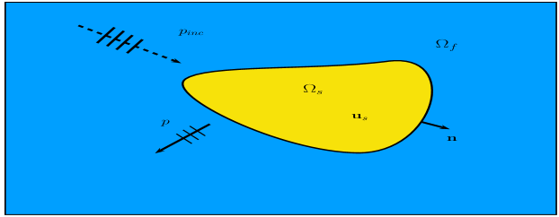
Figure 1: Schematic of the fluid-structure interaction problem.

Note that $\partial\Omega_{s}$, the bounded component of the boundary of $\Omega_{f}$ coincides with the boundary of the elastic body $\Omega_{s}$. We denote $\Gamma:=\partial\Omega_{f}=\partial\Omega_{s}$.

The parameters describing the elastic properties of $\Omega_{s}$ are the so-called Lamé constants $\mu>0$ and $\lambda\in\mathbb{R}$, satisfying the condition

$$\lambda+\left(\frac{2}{n}\right)\mu>0.$$ (2)

One fluid-structure interaction problem of interest concerns the situation when the fields are time-harmonic, allowing us to factor out the time-dependence and consider the problem in the frequency domain. Using standard interface conditions coupling the pressure in the fluid $p$ and the elastic displacement in the solid ${\bf u}$, the fluid-solid interaction problem in the frequency domain reads: given volumetric forces ${\bf f}$ and ${\bf g}$, and an incident pressure $p_{\rm inc}$, find a pressure field $p$ in $\Omega_{f}$ and elastic deformations ${\bf u}$ of $\Omega_{s}$ satisfying

$$\Delta p+\left(\frac{w^{2}}{c^{2}}\right)p={\rm div}\,{\bf f},\,\,\text{on $\Omega_{f}$},\quad-\rho w^{2}{\bf u}-{\bf div}\,\bm{\sigma}({\bf u})={\bf g},\,\,\text{in $\Omega_{s}$},$$ (3a)

$$-(p+p_{\rm inc}){\bf n}=\bm{\sigma}({\bf u}){\bf n},\quad\frac{\partial}{\partial{\bf n}}(p+p_{\rm inc})=\rho w^{2}{\bf u}\cdot{\bf n},\,\,\text{on $\Gamma$},$$ (3b)

$$\frac{\partial p}{\partial r}-i\left(\frac{w}{c}\right)p=o(1/r),\,\,\text{as $r:=\|{\bf x}\|\to\infty$}.$$ (3c)

The parameter $c$ is the constant speed of the sound in the fluid, and the Cauchy tensor $\bm{\sigma}$ depends on the Lamé constants $\mu>0$ and $\lambda\in\mathbb{R}$ and is defined in terms of the strain tensor $\bm{\varepsilon}({\bf u})$ as

$$\bm{\sigma}({\bf u}):=2\mu\bm{\varepsilon}({\bf u})+\lambda\,{\rm tr}(\bm{\varepsilon}({\bf u})){\bf I}\quad\text{in $\Omega_{s}$.}$$

Using the vector Laplacian operator, we see that

$${\rm\bf div}\,\bm{\sigma}({\bf u})=\mu\Delta{\bf u}+(\lambda+\mu)\nabla({\rm div}\,{\bf u})\quad\text{on $\Omega_{s}$}.$$

This is a commonly accepted formulation for time-harmonic fluid-solid interaction problems involving inviscid flow, see, for example, [15, 17, 18]. The system in Equation 3 is known to possess a non-trivial kernel under certain situations. As discussed in [19], this problem lacks a unique solution whenever ${\bf u}$ is a non-trivial solution of the homogeneous problem:

$$-{\bf div}\,\bm{\sigma}({\bf u})=\rho w^{2}{\bf u},\,\,\text{in $\Omega_{s}$},\quad\bm{\sigma}({\bf u}){\bf n}={\bf 0},\quad{\bf u}\cdot{\bf n}=0,\,\,\text{on $\Gamma$}.$$ (4)

The pair $(w^{2},{\bf u})$ solving this eigenvalue problem is a Jones eigenpair [19]. The homogeneous problem for the displacements can be viewed as the usual eigenvalue problem for linear elasticity with traction free boundary condition, plus the extra constraint on the normal trace of ${\bf u}$ along the boundary. Therefore, we may consider this as an overdetermined problem. We know that there is a countable number of eigenmodes for linear elasticity with free traction given reasonable assumptions on $\Gamma$ (see [2] and references therein). The extra condition ${\bf u}\cdot{\bf n}=0$ on the boundary plays an important role in the existence of the zero eigenvalue of Equation 4. All of these properties are discussed in detailed in the next sections.

We note that other authors have addressed the lack of uniqueness in Equation 3. A slightly different model for fluid-structure interaction in the frequency domain can be derived by considering the problem with non-zero fluid viscosity and then taking the viscosity to zero. As pointed out in [15], in this setting it is reasonable to adding another condition on the shear of ${\bf u}$ on the interface as a fix for the non-uniqueness of Equation 3. The condition

$$\rho w^{2}{\bf u}\cdot{\bf t}=\frac{\partial}{\partial{\bf t}}({\bm{\sigma}}({\bf u}){\bf n}\cdot{\bf n}),$$

removes the non-zero solutions of Equation 4. Here ${\bf t}$ is the unit tangent vector on $\Gamma$. In [9], the authors add a Robin boundary condition for the fluid pressure on a far enough “artificial” boundary containing the solid. They then consider the fluid to be bounded between the solid and this interface. As shown in the same reference, the modified problem has a unique solution.

Since our interest in the present paper concerns the eigenvalue problem Equation 1, we do not delve any further into the properties of the interaction problem (cf. Equation 3).

2.3 Lipschitz domains can support Jones modes

The paper by Hargé in 1990 [12] examined the existence of non-trivial solutions of Equation 1. The results of this paper have been cited extensively in subsequent works focusing on the well-posedness of the fluid-structure model presented in the previous section. As an instance, “Fortunately, these traction-free oscillations occur only in highly specific situations…” [16]; “Note that Hargé […] has established that Jones modes do not exist for arbitrarily-shaped bodies.” [3]; ”However, intuitively, we do not expect Jones frequencies to exist for an ”arbitrary” body; this has been proved recently by Hargé […]”. [23] These papers also note that domains which are axisymmetric may indeed have such modes. As a historical aside, Horace Lamb [21] documented such modes in the sphere in 1881.

Revisiting [12], we note that the setting of the paper is as follows:

Pour $\Omega$ ouvert borné connexe de $\mathbb{R}^{3}$ á bord $C^{\infty}$ … fixé et soit $E=\Big{\{}\phi\in C^{\infty}(\overline{\Omega};\mathbb{R}^{3});\,\phi\mbox{ diff\'{e}omorphisme de $\overline{\Omega}$ sur }\phi(\overline{\Omega})\Big{\}}$; on munit $E$ de la topologie $C^{\infty}$ …[12]

and the main theorem is then

There is an open, countable dense intersection $G$ of open sets of $E$ such that for any $\phi$ in $G$, there is no exceptional eigenvalue …

This theorem and its technique of proof cannot be directly applied to the situation of polygonal domains in $\mathbb{R}^{2}$, nor to polyhedral domains. Intuitively one may believe the result should hold in polygonal or polyhedral domains; indeed, our initial starting point for the current study was to try to extend the result of Hargé to general Lipschitz domains. The critical observation was the following example. It is easy to verify by inspection that $(w_{s}^{2},{\bf u}_{s}),(w_{p}^{2},{\bf u}_{p})$ defined below are Jones eigenpairs on the rectangle $[0,a]\times[0,b]$:

$${\bf u}_{s}:=\left((a\ell)\sin\Big{(}\frac{m\pi x}{a}\Big{)}\cos\Big{(}\frac{\ell\pi y}{b}\Big{)},-(bm)\cos\Big{(}\frac{m\pi x}{a}\Big{)}\sin\Big{(}\frac{\ell\pi y}{b}\Big{)}\right)^{\texttt{t}},$$ (5a)

$$w_{s}^{2}:=\frac{\mu\pi^{2}}{\rho}\left(\frac{m^{2}}{a^{2}}+\frac{\ell^{2}}{b^{2}}\right),\quad m,\ell=1,2,\ldots,$$ (5b)

and

$${\bf u}_{p}:=\left((bm)\sin\Big{(}\frac{m\pi x}{a}\Big{)}\cos\Big{(}\frac{\ell\pi y}{b}\Big{)},(a\ell)\cos\Big{(}\frac{m\pi x}{a}\Big{)}\sin\Big{(}\frac{\ell\pi y}{b}\Big{)}\right)^{\texttt{t}},$$ (6a)

$$w_{p}^{2}:=\frac{(\lambda+2\mu)\pi^{2}}{\rho}\left(\frac{m^{2}}{a^{2}}+\frac{\ell^{2}}{b^{2}}\right),\quad m,\ell=0,1,\ldots,\quad m+\ell>0.$$ (6b)

It can also be readily seen that ${{\rm div}\,{\bf u}_{s}}=0$ and ${\rm curl}\,{\bf u}_{p}=0$; eigenmodes of this form are termed $s$- and $p$- modes respectively. Further, some eigenvalues may have geometric multiplicity depending on $a$ and $b$. In case $\lambda,\mu,\frac{a^{2}}{b^{2}}$ are integers, the value $w^{2}$ can be a higher-multiplicity Jones eigenvalue with an associated eigenspace which includes both $s$- and $p$- modes, provided we can find integer pairs $(m,\ell)$ and $(n,k)$ satisfying

$$\frac{\mu\pi^{2}}{\rho}\left(\frac{m^{2}}{a^{2}}+\frac{\ell^{2}}{b^{2}}\right)=\frac{(\lambda+2\mu)\pi^{2}}{\rho}\left(\frac{n^{2}}{a^{2}}+\frac{k^{2}}{b^{2}}\right)=:w^{2}.$$

Studying this simple example it became clear that the situation for polygonal domains required a different approach, and would yield different results to those described in [12]. One could think, for example, that under certain conditions it could be possible for domains comprising a finite union of rectangles could possess Jones modes; this is shown to be the case for the L-shaped domain in a subsequent section.

3 Weak formulation

In the presence of corners or edges, it is no longer reasonable to ask for the boundary condition in the problem Equation 4 to be imposed pointwise, since the eigenfunctions may not be sufficiently regular. In fact, the zero normal trace condition on the displacement holds almost everywhere on $\partial\Omega$; it is clear that this condition cannot be imposed, for example over vertices of the boundary. A weak formulation is needed and later in this paper we shall compute Jones modes using a finite element discretization.

Let $\Omega$ be a Lipschitz domain of $\mathbb{R}^{n}$ (we drop the subscript referring to the solid domain). Recall the eigenvalue problem in Equation 4: find the Jones pairs $(w^{2},{\bf u})$, ${\bf u}$ non-zero, such that

$$-{\rm\bf div}\,\bm{\sigma}({\bf u}) =\rho w^{2}{\bf u},\quad\text{in $\Omega$},$$ (7a)

$$\bm{\sigma}({\bf u}){\bf n}={\bf 0}, \quad{\bf u}\cdot{\bf n}=0.\quad\text{on $\partial\Omega$}$$ (7b)

with $\rho>0$ a fixed constant. Using the definition of the Cauchy stress tensor, we can write Equation 7 as

$$\mu\Delta{\bf u}+(\lambda+\mu)\nabla({\rm div}{\bf u})+\rho w^{2}{\bf u} ={\bf 0}\quad\text{in $\Omega$,}$$ (8a)

$$\big{(}\mu\nabla{\bf u}+(\lambda+\mu)({\rm div}\,{\bf u}){\bf I}\big{)}{\bf n}={\bf 0},\,{\bf u}\cdot{\bf n} =0,\quad\text{on $\partial\Omega$.}$$ (8b)

In order to introduce a weak formulation of Equation 7 (equivalently Equation 8), we define the spaces

$${\bf H}^{1}(\Omega):=\Big{\{}{\bf v}=(v_{1},\ldots,v_{n}):\,v_{i}\in H^{1}(\Omega)\Big{\}},\quad{\bf H}:=\Big{\{}{\bf u}\in{\bf H}^{1}(\Omega):\,\gamma_{\bf n}{\bf u}=0\,\,\text{on $\partial\Omega$}\Big{\}}.$$

Here $H^{1}(\Omega)$ denotes the usual Hilbert space of scalar functions in $L^{2}(\Omega)$ whose partial derivatives (in all directions) belong to $L^{2}(\Omega)$. The operator $\gamma_{\bf n}:{\bf H}^{1}(\Omega)\to L^{2}(\partial\Omega)$ is the normal trace operator, which is linear and bounded in ${\bf H}^{1}(\Omega)$. The space ${\bf H}$ is endowed with the usual ${\bf H}^{1}$-inner product, denoted by $(\cdot,\cdot)_{1}$. This implies that ${\bf H}$ is a closed subspace of ${\bf H}^{1}(\Omega)$. We shall also need the space ${\bf H}^{t+1}(\Omega)$ of vector fields whose entries belong to the Sobolev space $H^{t+1}(\Omega),t\geq 0$, and the semi-norm $|\cdot|_{t+1}$ in ${\bf H}^{t+1}(\Omega)$.

We consider the following primal formulation of Equation 8: find ${\bf u}\in{\bf H}$ and $\kappa\in\mathbb{R}$ such that

$$a({\bf u},{\bf v})=\kappa\,({\bf u},{\bf v})_{0},\quad\forall\,{\bf v}\in{\bf H},$$ (9)

where $\kappa:=\rho w^{2}$, and the bilinear form $a:{\bf H}\times{\bf H}\to\mathbb{R}$ is given by

$$a({\bf u},{\bf v}):=\mu(\nabla{\bf u},\nabla{\bf v})_{0}+(\lambda+\mu)({\rm div}{\bf u},{\rm div}{\bf v})_{0},\quad\forall\,{\bf u},\,{\bf v}\in{\bf H},$$

Since ${\|{\rm div}{\bf u}\|_{0}\leq\|\nabla{\bf u}\|_{0}}\leq\|{\bf u}\|_{1}$, for all ${\bf u}\in{\bf H}^{1}(\Omega)$, the bilinear form $a(\cdot,\cdot)$ is bounded. In addition, $a(\cdot,\cdot)$ is symmetric and positive semi-definite. The Rayleigh quotient gives

$$\frac{a({\bf v},{\bf v})}{\|{\bf v}\|_{0}^{2}}\geq 0,\quad\forall\,{\bf v}\in{\bf H},\,{\bf v}\neq{\bf 0}.$$ (10)

We see that all possible eigenvalues of Equation 9 are real and non-negative. Using the Cauchy tensor ${\bm{\sigma}}$ we can write Equation 9 in the equivalent form

$$\tilde{a}({\bf u},{\bf v})=\kappa\,({\bf u},{\bf v})_{0},\quad\forall\,{\bf v}\in{\bf H},$$ (11)

where $\tilde{a}({\bf u},{\bf v}):=(\bm{\sigma}({\bf u}),\nabla{\bf v})_{0}=(\bm{\sigma}({\bf u}),\bm{\varepsilon}({\bf v}))_{0}$ for all ${\bf u},{\bf v}\in{\bf H}.$ In terms of the strain tensor only, $\tilde{a}(\cdot,\cdot)$ becomes

$$\tilde{a}({\bf u},{\bf v})=2\mu\big{(}{\bm{\varepsilon}}({\bf u}),{\bm{\varepsilon}}({\bf v})\big{)}_{0}+\lambda\big{(}{\rm tr}({\bm{\varepsilon}}({\bf u})),{\rm tr}({\bm{\varepsilon}}({\bf v}))\big{)}_{0}.$$

Using the deviatoric part of the strain tensor we can write

$$\tilde{a}({\bf u},{\bf v})=2\mu\big{(}{\bm{\varepsilon}}({\bf u})^{\texttt{d}},{\bm{\varepsilon}}({\bf v})^{\texttt{d}}\big{)}_{0}+\left(\lambda+\frac{2\mu}{n}\right)\big{(}{\rm tr}({\bm{\varepsilon}}({\bf u})),{\rm tr}({\bm{\varepsilon}}({\bf v}))\big{)}_{0},\quad\forall\,{\bf u},\,{\bf v}\in{\bf H}.$$ (12)

Obviously, $a({\bf u},{\bf v})=\tilde{a}({\bf u},{\bf v})$ for all ${\bf u},\,{\bf v}\in{\bf H}$. Furthermore, the bilinear forms $a(\cdot,\cdot)$ and $\tilde{a}(\cdot,\cdot)$ are bounded in ${\bf H}^{1}(\Omega)\times{\bf H}^{1}(\Omega)$ and hence in ${\bf H}\times{\bf H}$. We can then define the solution operator $\tilde{T}:{\bf L}^{2}(\Omega)\to{\bf H}$ by $\tilde{T}({\bf f})={\bf u}$ such that

$$\tilde{a}({\bf u},{\bf v})=({\bf f},{\bf v})_{0},\quad\forall\,{\bf v}\in{\bf H}.$$ (13)

We immediately have that $\tilde{T}$ is a linear operator. However, to show all necessary properties of $\tilde{T}$, we need to show that $\tilde{a}$ (equivalent $a$) is coercive in ${\bf H}$. In particular, this will give us the compactness of $\tilde{T}$ restricted to ${\bf H}$, and therefore we are guaranteed that $\tilde{T}$ has a countable and positive point spectrum with eigenfunctions lying in ${\bf H}$. These properties will rely on the coercivity properties of $\tilde{a}(\cdot,\cdot)$, which will depend crucially on the domain shape as we shall see.

Using the definition of $\tilde{a}(\cdot,\cdot)$, for any ${\bf u}\in{\bf H}$ we have

$$\tilde{a}({\bf u},{\bf u})= \,2\mu\|{\bm{\varepsilon}}({\bf u})^{\texttt{d}}\|_{0}^{2}+\left(\lambda+\frac{2\mu}{n}\right)\|{\rm tr}({\bm{\varepsilon}}({\bf u}))\|_{0}^{2}$$

$$= \,n\Big{(}\frac{2\mu}{n}\|{\bm{\varepsilon}}({\bf u})^{\texttt{d}}\|_{0}^{2}+\left(\lambda+\frac{2\mu}{n}\right)\frac{1}{n}\|{\rm tr}({\bm{\varepsilon}}({\bf u}))\|_{0}^{2}\Big{)}$$

$$\geq \,\min\Big{\{}2\mu,n\left(\lambda+\frac{2\mu}{n}\right)\Big{\}}\Big{(}\|{\bm{\varepsilon}}({\bf u})^{\texttt{d}}\|_{0}^{2}+\frac{1}{n}\|{\rm tr}({\bm{\varepsilon}}({\bf u}))\|_{0}^{2}\Big{)}$$

$$= \,\min\Big{\{}2\mu,n\left(\lambda+\frac{2\mu}{n}\right)\Big{\}}\|{\bm{\varepsilon}}({\bf u})\|_{0}^{2},$$

where we have used $\|{\bm{\tau}}\|_{0}^{2}=\|{\bm{\tau}}^{\texttt{d}}\|_{0}^{2}+\frac{1}{n}\|{\rm tr}({\bm{\tau}})\|_{0}^{2}$. This establishes the inequality

$$\tilde{a}({\bf u},{\bf u})\geq \,\min\Big{\{}2\mu,n\left(\lambda+\frac{2\mu}{n}\right)\Big{\}}\|{\bm{\varepsilon}}({\bf u})\|_{0}^{2},\quad\forall\,{\bf u}\in{\bf H}.$$ (14)

Now, to show that $\tilde{a}(\cdot,\cdot)$ is coercive on ${\bf H}$, we need to bound from below the term $\|{\bm{\varepsilon}}({\bf u})\|_{0}$ by $\|{\bf u}\|_{1}$ (up to a constant). However, as we will see in the forthcoming sections, the intersection ${\bf R}{\bf M}(\Omega)\cap{\bf H}$ depends intimately on $\Omega$ and therefore the positiveness of $\tilde{a}(\cdot,\cdot)$ cannot be established in case this intersection is not the trivial space.

It turns out that for non-axisymmetric Lipschitz domains, $\kappa=0$ is not in the point spectrum of Equation 11. We establish this in the following subsection.

3.1 Existence of Jones modes on non-axisymmetric domains

Let $\Omega$ be a non-axisymmetric domain in $\mathbb{R}^{n},\,n\in\{2,3\}$. In [4] the following version of Korn’s inequality for vector fields in ${\bf H}$ defined on non-axisymmetric Lipschitz domains was established: there is a positive constant $C$ which depends only on $\Omega$ so that

$$\|{\bm{\varepsilon}}({\bf u})\|_{0}\geq C\|{\bf u}\|_{1},\quad\forall\,{\bf u}\,\in{\bf H}.$$ (15)

This is a type of Korn’s inequality; we recall there are several variants of this inequality, [14].

Combining the inequality above and the derived inequality for $\tilde{a}(\cdot,\cdot)$ in Equation 14 we obtain the coercivity of $\tilde{a}(\cdot,\cdot)$ in ${\bf H}$ for non-axisymmetric domains:

$$\tilde{a}({\bf u},{\bf u})\geq \,C^{2}\min\Big{\{}2\mu,d\left(\lambda+\frac{2\mu}{n}\right)\Big{\}}\|{\bf u}\|_{1}^{2},\quad\forall\,{\bf u}\in{\bf H}.$$ (16)

Provided $\Omega$ is a non-axisymmetric Lipschitz domain, the coercivity of $\tilde{a}(\cdot,\cdot)$ means that the solution operator $\tilde{T}|_{\bf H}:{\bf H}\rightarrow{\bf H}$ is well-defined, and satisfies

$$C^{2}\min\Big{\{}2\mu,d\left(\lambda+\frac{2\mu}{n}\right)\Big{\}}\|\tilde{T}{\bf f}\|_{1}^{2}\leq{\tilde{a}(\tilde{T}{\bf f},\tilde{T}{\bf f})=({\bf f},\tilde{T}{\bf f})_{0}}\leq\|\tilde{T}{\bf f}\|_{0}\|{\bf f}\|_{0},$$

for all ${\bf f}\in{\bf H}$. This establishes the boundedness of $\tilde{T}$:

$$\|\tilde{T}{\bf f}\|_{1}\leq\frac{C^{-2}}{\min\Big{\{}2\mu,d\left(\lambda+\frac{2\mu}{n}\right)\Big{\}}}\|{\bf f}\|_{l},\quad l\in\{0,1\},\,\forall\,{\bf f}\in{\bf H}.$$ (17)

The compactness of the inclusion ${\bf H}^{1}(\Omega)\hookrightarrow{\bf L}^{2}(\Omega)$, and the fact that ${\bf H}$ is closed in ${\bf H}^{1}(\Omega)$, imply that ${\bf H}$ is continuously embedded in ${\bf H}^{1}(\Omega)$, and hence that the inclusion ${\bf H}\hookrightarrow{\bf L}^{2}(\Omega)$ is compact. Therefore, the previous bound with $l=0$ imply the compactness of $\tilde{T}|_{\bf H}$. The Spectral Theorem for bounded self-adjoint linear and compact operators says that $\tilde{T}$ has a countable real point spectrum $\{{\alpha_{n}}\}\subseteq(0,{\|\tilde{T}\|})$ and eigenfunctions $\{{\bf u}_{n}\}$ such that $\tilde{T}{\bf u}_{n}={\alpha_{n}}{\bf u}_{n}$ for all $n$, with $\|\tilde{T}\|:=C^{-2}\min\Big{\{}2\mu,d\left(\lambda+\frac{2\mu}{n}\right)\Big{\}}^{-1}$. Note that the eigenpair $({\alpha_{n}},{\bf u}_{n})$ of $\tilde{T}$ solves Equation 11 with $\kappa_{n}=\frac{1}{\alpha_{n}}$ and ${\bf u}_{n}$ as the corresponding eigenfunction.

We remark that the results in this section also hold for the bilinear form $a(\cdot,\cdot)$ and therefore, since $\tilde{a}({\bf u},{\bf v})=a({\bf u},{\bf v})$ for all ${\bf u},\,{\bf v}\in{\bf H}$, this establishes the existence of the Jones spectrum for bounded Lipschitz domains $\Omega$ which are not axisymmetric.

To finish up this section, we summarize the main properties in the following theorem.

Theorem 1.

Let us assume $\Omega$ is a non-axisymmetric and Lipschitz domain of $\mathbb{R}^{n}$, $n\in\{2,3\}$. The spectrum of $\tilde{T}$ is $\{{\alpha_{n}}\}_{n\in\mathbb{N}}\subseteq(0,\|\tilde{T}\|)$, with eigenfunctions belonging to ${\bf H}$. In addition, eigenfunctions corresponding to different eigenvalues are orthogonal in the usual ${\bf L}^{2}$-inner product.

3.2 The case of zero eigenvalues and rigid motions

When studying problems involving the Lamé operator $\mathcal{L}$ (cf. section 1), we need to be aware of rigid motions. Depending on the boundary conditions imposed, rigid motions may be part of the eigenspace of certain eigenvalues. Rigid motions satisfy $\mathcal{L}{\bf w}={\bf 0}$, and it is possible that they may satisfy both Equation 1b and Equation 1c. We now want to characterize domains having these eigenfunctions. Consider the space

$${\bf R}{\bf M}(\Omega):=\{{\bf u}\in{\bf H}^{1}(\Omega):\,{\bf u}={\bf b}+{\bf B}{\bf x},\,\,{\bf b}\in\mathbb{R}^{n},\,{\bf B}\in\mathbb{R}^{n\times n}_{skew},\,{\bf x}\in\Omega\},$$

where $\mathbb{R}^{n\times n}_{skew}$ is the space of all skew-symmetric matrices in $\mathbb{R}^{n\times n}$. The space ${\bf R}{\bf M}(\Omega)$ consists of translations, rotations and combinations of these. It is known that (see, e.g. [2] and references therein) the linear elasticity problem with traction free boundary conditions

$$-{\bf div}\,{\bm{\sigma}}(\bar{\bf u})=\delta\bar{\bf u},\quad\text{in $\Omega$},\quad{\bm{\sigma}}(\bar{\bf u}){\bf n}={\bf 0},\quad\text{in $\partial\Omega$},$$ (18)

has eigenmodes in ${\bf R}{\bf M}(\Omega)$ with eigenvalue $\delta=0$. In fact, if $n=2$, the eigenspace of $\delta=0$ is exactly ${\bf R}{\bf M}(\Omega)$ with dimension 3. Define now the space

$${\bf Z}:=\Big{\{}{\bf u}\in{\bf H}^{1}(\Omega):\,\tilde{a}({\bf u},{\bf v})=0,\,\,\forall\,{\bf v}\in{\bf H}^{1}(\Omega)\Big{\}}.$$

Examining the weak formulation of Equation 18, it is clear that ${\bf R}{\bf M}{(\Omega)}\subseteq{\bf Z}$. We show that these spaces actually coincide.

Theorem 2.

There holds ${\bf R}{\bf M}(\Omega)={\bf Z}$.

Proof.

First, let ${\bf u}\in{\bf R}{\bf M}(\Omega)$. By definition, ${\bf u}={\bf b}+{\bf B}{\bf x}$, ${\bf x}\in\Omega$, ${\bf B}$ skew-symmetric. Then $\nabla{\bf u}={\bf B}$ so that ${\bm{\varepsilon}}({\bf u})={\bf 0}$ and clearly $\tilde{a}({\bf u},{\bf v})=0$ for any ${\bf v}\in{\bf H}^{1}(\Omega)$. Conversely, assume ${\bf u}\in{\bf Z}$. Then $\tilde{a}({\bf u},{\bf u})=0$, and using the definition of $\tilde{a}(\cdot,\cdot)$ in Equation 12 we get

$$0=2\mu{\rm tr}({\bm{\varepsilon}}({\bf u}))+n\lambda{\rm tr}({\bm{\varepsilon}}({\bf u}))=n\left(\lambda+\frac{2}{n}\mu\right){\rm tr}({\bm{\varepsilon}}({\bf u})).$$

Since $\lambda+\frac{2}{n}\mu>0$, we get that both ${\rm tr}({\bm{\varepsilon}}({\bf u}))=0$ and ${\bm{\varepsilon}}({\bf u})={\bf 0}$. This implies that ${\bf u}\in{\bf R}{\bf M}(\Omega)$. ∎

Now that we know the eigenvalue problem in Equation 18 has ${\bf R}{\bf M}(\Omega)$ as the eigenspace of $\delta=0$, the question is if there is any non-zero elements in ${\bf R}{\bf M}(\Omega)\cap{\bf H}$, i.e., those which satisfy the additional constraint ${\bf u}\cdot{\bf n}=0$ on the boundary. Such elements would be Jones modes corresponding to a zero Jones eigenvalue.

The next result states the cases in which we have 2D rigid motions which additionally satisfy ${\bf u}\cdot{\bf n}=0$ on the boundary. We note parts (i) and (ii) of the result can be combined for a more succinct statement involving arbitrary half-spaces, but we provide the version below for clarity of exposition.

Theorem 3.

Assume $n=2$. If $\Omega$ is not bounded, then

• ${\bf R}{\bf M}(\Omega)\cap{\bf H}={\rm span}\{(0,1)^{\texttt{t}}\}$ if and only if $\Omega=\{(x,y)^{\texttt{t}}\in\mathbb{R}^{2}:\,x>a,y\in\mathbb{R}\}$, for $a\in\mathbb{R}$.

• ${\bf R}{\bf M}(\Omega)\cap{\bf H}={\rm span}\{(1,0)^{\texttt{t}}\}$ if and only if $\Omega=\{(x,y)^{\texttt{t}}\in\mathbb{R}^{2}:\,x\in\mathbb{R},y>b\}$, for $b\in\mathbb{R}$.

In case $\Omega$ is bounded,

• ${\bf R}{\bf M}(\Omega)\cap{\bf H}={\rm span}\{(y,-x)^{\texttt{t}}\}$ if and only if $\Omega=B(0,R)$.

Proof.

For (i), suppose $\Omega=\{(x,y)^{\texttt{t}}\in\mathbb{R}^{2}:\,x>a,y\in\mathbb{R}\}$, for some $a\in\mathbb{R}$. Let ${\bf u}\in{\bf R}{\bf M}(\Omega)\cap{\bf H}$. We write ${\bf u}={\bf b}+{\bf B}{\bf x}$, ${\bf b}\in\mathbb{R}^{2}$, ${\bf B}$ skew-symmetric, and ${\bf x}\in\Omega$. Assume

$${\bf b}=(b_{1},b_{2})^{\texttt{t}},\quad{\bf B}=\left(\begin{array}[]{cc}0&b\\ -b&0\end{array}\right).$$

The normal on $\partial\Omega:=\{(a,y):\,y\in\mathbb{R}\}$ is ${\bf n}=(-1,0)^{\texttt{t}}$. We have

$$0={\bf u}\cdot{\bf n}={\bf b}\cdot{\bf n}+{\bf B}{\bf x}\cdot{\bf n}=b_{1}+by,\quad\forall\,y\in\mathbb{R}.$$

We must have $b_{1}=0$ and $b=0$, which gives ${\bf B}={\bf 0}$ and ${\bf b}=(0,b_{2})$, showing that ${\bf u}\in{\rm span}\{(0,1)^{\texttt{t}}\}$. Part (ii) can be easily proved by following the same steps showed before. For (iii), assume $\Omega$ is a circle of radius $R$ centered at the origin. Let ${\bf u}\in{\bf R}{\bf M}(\Omega)\cap{\bf H}$. As before, ${\bf u}={\bf b}+{\bf B}{\bf x}$, ${\bf x}\in\Omega$, and ${\bf u}\cdot{\bf n}=0$ on $\partial\Omega=\{(x,y)\in\mathbb{R}^{2}:\,x^{2}+y^{2}=R^{2}\}$. Then

$$0={\bf u}\cdot{\bf n}={\bf b}\cdot{\bf n}+{\bf B}{\bf x}\cdot{\bf n}=b_{1}n_{1}+b_{2}n_{2}+b(n_{1}y-n_{2}x),\quad\forall\,(x,y)\in\partial\Omega.$$

The normal vector on $\partial\Omega$ is ${\bf n}=\frac{1}{R}(x,y)$. Putting this into the previous equation we obtain

$$b_{1}x+b_{2}y=0,\quad\forall\,(x,y)\in\partial\Omega.$$

Since $x$ and $y$ cannot be zero simultaneously, we conclude that $b_{1}=b_{2}=0$ and ${\bf u}={\bf B}{\bf x}$, proving that ${\bf u}\in{\rm span}\{(y,-x)^{\texttt{t}}\}$.

Note that the converses of all three parts (i), (ii) and (iii) are trivial since the basis of ${\bf R}{\bf M}(\Omega)\cap{\bf H}$ is always orthogonal (in the Euclidean inner product) to the normal vector on the boundary of the corresponding domain. ∎

In the result above one could also have the same conclusions for the complement of each domain considered. Indeed, the complement of $\Omega$ in parts (i), (ii) and (iii) obviously has the same boundary $\partial\Omega$, meaning that the normal vector only changes its sign. This indicates that the vanishing condition of the normal trace of the displacement would be readily satisfied in this case as well.

Theorem 2 suggests that the traction eigenvalue problem given by Equation 18 has zero as eigenvalue with rigid motions as eigenfunctions, independent of the domain $\Omega$. However, the extra constraint on the normal trace of the displacement ${\bf u}$ (cf. Equation 4) may preclude $\kappa=0$ as a Jones eigenvalue on some domains. The elements in ${\bf R}{\bf M}(\Omega)\cap{\bf H}$ depend on the boundary of $\Omega$ as shown in Theorem 3. Combining Theorem 2 and Theorem 3, we have the following theorem.

Theorem 4.

Assume $n=2$ and suppose $\kappa=0$ in Equation 9 (equivalently Equation 11). If $\Omega$ is not bounded, then

• ${\bf u}_{0}=(0,1)^{\texttt{t}}$ is a Jones mode on $\Omega:=\{(x,y)^{\texttt{t}}\in\mathbb{R}^{2}:\,x>a,y\in\mathbb{R}\}$, for some $a\in\mathbb{R}$.

• ${\bf u}_{0}=(1,0)^{\texttt{t}}$ is a Jones mode on $\Omega:=\{(x,y)^{\texttt{t}}\in\mathbb{R}^{2}:\,x\in\mathbb{R},y>b\}$, for some $b\in\mathbb{R}$.

In case $\Omega$ is bounded, then

• ${\bf u}_{0}=(y,-x)^{\texttt{t}}$ is a Jones mode on $\Omega:=B(0,R)$, for any fixed $0<R<\infty$.

In the 3D case, a rigid motion can be decomposed as

$${\bf u}= \,c_{1}(1,0,0)^{\texttt{t}}+c_{2}(y,-x,0)^{\texttt{t}}+c_{3}(z,0,-x)^{\texttt{t}}+c_{4}(0,1,0)^{\texttt{t}}$$

$$+c_{5}(0,z,-y)^{\texttt{t}}+c_{6}(0,0,1)^{\texttt{t}},$$

for constants $c_{1},\ldots,c_{6}\in\mathbb{R}$. In this case, we see that we have three possible rotations and three possible translations. This implies that we may have more eigenvectors associated to the zero eigenvalue in Equation 9 (equivalently Equation 11).

The spaces ${\bf T}(\Omega)$ and ${\bf R}(\Omega)$ are defined as the spaces of pure translations and pure rotations of $\Omega$ respectively. These allow the following decomposition of ${\bf R}{\bf M}(\Omega)$:

$${\bf R}{\bf M}(\Omega)={\bf T}(\Omega)\oplus{\bf R}(\Omega),$$

with trivial intersection. To characterize the elements of ${\bf R}{\bf M}(\Omega)\cap{\bf H}$, it was shown in [4] that axisymmetric domains always support rotational displacements in ${\bf R}(\Omega)$ which are tangential to the boundary.

3D versions of Theorem 3 and Theorem 4 can be now stated.

Theorem 5.

Assume $n=3$. If $\Omega$ is not bounded, then

• ${\bf R}{\bf M}(\Omega)\cap{\bf H}={\rm span}\{(1,0,0)^{\texttt{t}}\}$ if $\Omega:=\{(x,y,z)^{\texttt{t}}\in\mathbb{R}^{3}:\,by+cz<a,x\in\mathbb{R}\}$, for some $a,b,c\in\mathbb{R}$ such that $1=b^{2}+c^{2}$.

• ${\bf R}{\bf M}(\Omega)\cap{\bf H}={\rm span}\{(0,1,0)^{\texttt{t}}\}$ if $\Omega:=\{(x,y,z)^{\texttt{t}}\in\mathbb{R}^{3}:\,ax+cz<b,y\in\mathbb{R}\}$, for some $a,b,c\in\mathbb{R}$ such that $1=a^{2}+c^{2}$.

• ${\bf R}{\bf M}(\Omega)\cap{\bf H}={\rm span}\{(0,0,1)^{\texttt{t}}\}$ if $\Omega:=\{(x,y,z)^{\texttt{t}}\in\mathbb{R}^{3}:\,ax+by<c,z\in\mathbb{R}\}$, for some $a,b,c\in\mathbb{R}$ such that $1=a^{2}+b^{2}$.

In case $\Omega$ is bounded,

• ${\bf R}{\bf M}(\Omega)\cap{\bf H}\subseteq{\bf R}(\Omega)$ if and only if $\Omega$ is axisymmetric.

Proof.

(i), (ii) and (iii) readily follow by applying the same steps as in the proof of parts (i) and (ii) of Theorem 3. For part (iv), let ${\bf u}\in{\bf R}{\bf M}(\Omega)\cap{\bf H}\subseteq{\bf R}(\Omega)$, and assume $\Omega$ is a non-axisymmetric domain. Then, Korn’s inequality (cf. inequality Equation 15) holds for ${\bf u}$, that is, there is a constant $c>0$ such that $c\|{\bf u}\|_{1}\leq\|{\bm{\varepsilon}}({\bf u})\|_{0}$. However, ${\bf u}\in{\bf R}(\Omega)$ is a rotation so ${\bm{\varepsilon}}({\bf u})={\bf 0}$ and $\|{\bf u}\|_{1}\neq 0$. This means that $c\leq 0$, which is a contradiction. For the converse of part(iv), assume that $\Omega$ is axisymmetric, and ${\bf R}(\Omega)\subseteq{\bf R}{\bf M}(\Omega)\cap{\bf H}$ with strict inclusion. This implies there is an element of ${\bf R}{\bf M}(\Omega)\cap{\bf H}$ which is a non-zero translation motion; however, the boundary condition on the normal trace prohibits such modes. ∎

From here, Theorem 2 and Theorem 5 give the next result.

Theorem 6.

Assume $n=3$ and suppose $\kappa=0$ is an eigenvalue of Equation 7. If $\Omega$ is not bounded, then its corresponding eigenvector is:

• ${\bf u}_{0}=(1,0,0)^{\texttt{t}}$ on $\Omega:=\{(x,y,z)^{\texttt{t}}\in\mathbb{R}^{3}:\,by+cz<a,x\in\mathbb{R}\}$, for some $a,b,c\in\mathbb{R}$ such that $1=b^{2}+c^{2}$.

• ${\bf u}_{0}=(0,1,0)^{\texttt{t}}$ on $\Omega:=\{(x,y,z)^{\texttt{t}}\in\mathbb{R}^{3}:\,ax+cz<b,y\in\mathbb{R}\}$, for some $a,b,c\in\mathbb{R}$ such that $1=a^{2}+c^{2}$.

• ${\bf u}_{0}=(0,0,1)^{\texttt{t}}$ on the domain $\Omega:=\{(x,y,z)^{\texttt{t}}\in\mathbb{R}^{3}:\,ax+by<c,z\in\mathbb{R}\}$, for some $a,b,c\in\mathbb{R}$ such that $1=a^{2}+b^{2}$.

In case $\Omega$ is bounded, its corresponding eigenvector is

• ${\bf u}_{0}\in{\bf R}(\Omega)$ whenever $\Omega$ is axisymmetric.

In the case of the circle in 2D, the zero eigenvalue would lead to a bilinear form $a(\cdot,\cdot)$ that is not ${\bf H}$-elliptic. For the 3D case, axisymmetric domains would lead to a loss of ${\bf H}$-ellipticity for the bilinear form $a(\cdot,\cdot)$. To overcome this issue, we add a shift to the formulation in Equation 9 to get the equivalent formulation: find $({\bf u},\kappa)\in{\bf H}\times\mathbb{R}$ such that

$$\bar{a}({\bf u},{\bf v})=(\kappa+1)({\bf u},{\bf v})_{0},\quad\forall\,{\bf v}\in{\bf H},$$ (19)

with $\bar{a}({\bf u},{\bf v}):=a({\bf u},{\bf v})+({\bf u},{\bf v})_{0},$ for all ${\bf u},\,{\bf v}\in{\bf H}$. This new formulation is obviously ${\bf H}$-elliptic since for any ${\bf u}\in{\bf H}$ we have

$$\bar{a}({\bf u},{\bf v})=\mu\|\nabla{\bf u}\|_{0}^{2}+(\lambda+\mu)\|{\rm div}\,{\bf u}\|_{0}^{2}+\|{\bf u}\|_{0}^{2}\geq\min\{\mu,1\}\|{\bf u}\|_{1}^{2}.$$

The symmetry of $a(\cdot,\cdot)$ and the inner product $(\cdot,\cdot)_{0}$ along with the Rayleigh quotient (cf. Equation 10) show that the eigenvalues $\kappa+1$ of Equation 19 are real and positive.

We define the solution operator $\bar{T}:{\bf L}^{2}(\Omega)\to{\bf H}$ by $\bar{T}({\bf f})={\bf u}$ such that

$$\bar{a}({\bf u},{\bf v})=({\bf f},{\bf v})_{0},\quad\forall\,{\bf v}\in{\bf H},$$ (20)

Since $\bar{a}(\cdot,\cdot)$ is ${\bf H}$-elliptic, the Lax-Milgram lemma shows that the restriction of $\bar{T}$ to ${\bf H}$, $\bar{T}|_{\bf H}$, is a well-defined linear operator and also gives the boundedness of $\bar{T}|_{\bf H}$ in the ${\bf L}^{2}$- and ${\bf H}^{1}$-norms:

$$\|\bar{T}{\bf f}\|_{1}\leq\frac{1}{\min\{\mu,1\}}\|{\bf f}\|_{l},\quad l\in\{0,1\},\,\,\forall\,{\bf f}\in{\bf H}.$$ (21)

We again use the compact inclusion ${\bf H}^{1}(\Omega)\hookrightarrow{\bf L}^{2}(\Omega)$ to obtain the compactness of the inclusion ${\bf H}\hookrightarrow{\bf L}^{2}(\Omega)$. This compact inclusion and the bound of $\bar{T}|_{\bf H}$ in Equation 21 with $l=0$ imply that $\bar{T}$ is a compact operator (see [2]). Also, the symmetry of $\bar{a}(\cdot,\cdot)$ implies that $\bar{T}$ is a self-adjoint with respect to $\bar{a}(\cdot,\cdot)$. The Spectral Theorem for compact and self-adjoint bounded linear operators now implies the existence of positive eigenvalues $\{{\beta_{n}}\}_{n\in\mathbb{N}}$ and eigenfunctions $\{{\bf u}_{n}\}_{n\in\mathbb{N}}$ such that $\bar{T}{\bf u}_{n}={\beta_{n}}{\bf u}_{n}$ and ${\beta_{n}}\to 0$. Note that $\bar{T}{\bf u}_{n}={\beta_{n}}{\bf u}_{n}$ is a solution of Equation 20 if and only if $(\kappa_{n},{\bf u}_{n})$ solves Equation 9 with ${\beta_{n}}:=\frac{1}{\kappa_{n}+1}$. Since $\kappa_{n}\geq 0$ for any $n\in\mathbb{N}$, we see that $\{{\beta_{n}}\}_{n\in\mathbb{N}}\subseteq(0,1]$. We summarize these properties in the following main result.

Theorem 7.

The point spectrum of $\bar{T}|_{\bf H}$ is decomposed as follows: $\{{\beta_{n}}\}_{n\in\mathbb{N}}\cup\{1\}$, where

1. the associated eigenspace of the eigenvalue 1 is given by Theorem 3 in 2D and Theorem 5 in 3D;

2. $\{{\beta_{n}}\}_{n\in\mathbb{N}}\subseteq(0,1)$ is a sequence of eigenvalues of $\bar{T}$ with finite multiplicity that converges to 0 and their corresponding eigenfunctions lie in ${\bf H}$.

In addition, eigenfunctions corresponding to different eigenvalues are orthogonal in the usual ${\bf L}^{2}$-inner product.

3.3 Elastic bodies with variable density

In many realistic applications the density $\rho>0$ varies. In this section we discuss the existence of Jones eigenpairs for variable density. Under the same assumptions on $\Omega$ as given at the beginning of section 3, we consider a variable density $\rho>0$ belonging to $L^{\infty}(\Omega)$. The weak formulation in Equation 9 would then be: find Jones eigenpairs ${\bf u}\in{\bf H}$ and $w^{2}\in\mathbb{R}$ such that

$$a({\bf u},{\bf v})=w^{2}\,b({\bf u},{\bf v}),\quad\forall\,{\bf v}\in{\bf H},$$ (22)

where the bilinear form $b(\cdot,\cdot)$ is defined as

$$b({\bf u},{\bf v}):=\int_{\Omega}\rho\,{\bf u}\cdot{\bf v},\quad\forall\,{\bf u},\,{\bf v}\in{\bf H}.$$

Since $\rho\in L^{\infty}(\Omega)$, we have that $|b({\bf u},{\bf v})|\leq\|\rho\|_{\infty}\|{\bf u}\|_{0}\|{\bf v}\|_{0},$ for all ${\bf u},\,{\bf v}\in{\bf H}$. If $L^{2}_{\rho}(\Omega)$ denotes the space of functions in $L^{2}(\Omega)$ whose weighted inner product is finite (with the variable density as the corresponding weight), we note that the inclusion ${\bf H}\hookrightarrow L^{2}_{\rho}(\Omega)$ is compact.

The fact that the density varies does not change the positiveness of $a(\cdot,\cdot)$ (equivalently $\tilde{a}(\cdot,\cdot)$) in ${\bf H}$. We then have that the ${\bf H}$-ellipticity in Equation 16 holds true in this case as well.

We can conclude that the existence of Jones eigenpairs is guaranteed by Theorem 1 and Theorem 2 for the non-axisymmetric and the axisymmetric case, respectively. However, eigenfunctions corresponding to different eigenvalues would be orthogonal in the weighted inner product as defined by the bilinear form $b(\cdot,\cdot)$.

We end this section by summarizing our main results. For axisymmetric domains, Jones modes exist and include 0 as an eigenvalue with certain rigid motions as permissible eigenmodes. For non-axisymmetric Lipschitz domains which are bounded, there are countably many positive Jones eigenvalues whose only accumulation point is at infinity. Finally, if a variable density of the elastic body is assumed, then the existence of eigenpairs falls into the setup of Theorem 1 and Theorem 7, depending on the nature of the shape of the domain.

In the forthcoming section we use a standard conforming finite element method to approximate Jones eigenmodes. As per usual of this approach, one has that at a given level of refinement, curved boundaries are approximated by straight edges and/or faces. Numerically speaking, this means that, in the case of an axisymmetric domain, the numerical method may not compute the zero eigenvalue which should be a Jones eigenvalue as shown in Theorem 7. As we will see in section 5, even in the most simple case the standard conforming finite element method used for non-axisymmetric domain might not be a suitable choice to approximate Jones eigenpairs on axisymmetric domains.

4 Discrete weak formulations

The preceding discussion shows that the behaviour of Jones modes for axisymmetric and non-axisymmetric domains is different. We now present discretization strategies for both. Even though two discrete formulations are given for the Jones eigenproblem, we only provide a priori error estimates on polygons or polyhedra since, as the results presented in subsection 5.3 below suggest that the discrete formulation in Equation 23 does not appear to approximate the Jones eigenvalues correctly on curvilinear domains.

We first let $\Omega$ be a polygonal/polyhedral domain in $\mathbb{R}^{n},$ with $n\in\{2,3\}$, and let $\mathbb{T}_{h}$ be a regular triangulation by triangles (tetrahedra in 3D) of $\overline{\Omega}$ with meshsize $h$. For a given integer $k\geq 1$, we consider the space ${\bf P}_{k}(T)$ as the set of all vector polynomials of degree at most $k$ defined on $T\in\mathbb{T}_{h}$. Define the space

$${\bf H}_{h}:=\Big{\{}{\bf v}_{h}\in{{\bf C}}(\overline{\Omega}):\,{\bf v}_{h}|_{T}\in{\bf P}_{k}(T),\,\,\forall\,T\in\mathcal{T}_{h}\Big{\}}\cap{\bf H},$$

where ${\bf C}(\overline{\Omega})$ is the space of continuous vector fields defined over $\overline{\Omega}$. Consider the discrete weak formulation: find ${\bf u}_{h}\in{\bf H}_{h}$ and $\kappa_{h}\in\mathbb{R}$ such that

$$a({\bf u}_{h},{\bf v}_{h})=\kappa_{h}\,({\bf u}_{h},{\bf v}_{h})_{0},\quad\forall\,{\bf v}_{h}\in{\bf H}_{h}.$$ (23)

From the discussion in Sections 2 and 3, for non-axisymmetric domains the bilinear forms $\tilde{a}(\cdot,\cdot)$ and $a(\cdot,\cdot)$ coincide in ${\bf H}$. We only provide approximation results for the eigenvalue problem Equation 9 as they readily apply to the formulations Equation 11 and Equation 19.

Since ${\bf H}_{h}$ is a subspace of ${\bf H}$, the coercivity of $a(\cdot,\cdot)$ (cf. inequality Equation 16) in ${\bf H}$ implies its ${\bf H}_{h}$-ellipticity. We can define a discrete solution operator $T_{h}$ as follows:

$$T_{h}:\, {\bf L}^{2}(\Omega)\to{\bf H}_{h}$$

$${\bf f}\to T_{h}({\bf f}):={\bf u}_{h},$$

where ${\bf u}_{h}\in{\bf H}_{h}$ is the solution of the problem

$$a({\bf u}_{h},{\bf v}_{h})=({\bf f},{\bf v}_{h}){{}_{0}}\quad\forall\,{\bf v}_{h}\in{\bf H}_{h}.$$

Analogous to the situation of the continuous weak formulation, the pair $(\kappa_{h},{\bf u}_{h})$ solves Equation 23 if and only if $T_{h}{\bf u}_{h}=\sigma_{h}{\bf u}_{h}$ and $\sigma_{h}:=\frac{1}{\kappa_{h}}$. Also, the restriction operator $T_{h}|_{{\bf H}_{h}}:\,{\bf H}_{h}\to{\bf H}_{h}$ is self-adjoint with respect to $a(\cdot,\cdot)$ and $(\cdot,\cdot)_{0}$. We thus have the following result concerning the spectrum of $T_{h}|_{{\bf H}_{h}}$ on non-axisymmetric Lipschitz domains.

Theorem 8.

The spectrum of $T_{h}|_{{\bf H}_{h}}$ consists of $M_{h}:=\dim({\bf H}_{h})$ eigenvalues. Moreover,

1. the point spectrum consists of positive eigenvalues $\{\sigma_{h,k}\}_{k=1}^{M_{h}}$ counted with their multiplicities;

2. $\sigma_{h}=0$ is not an eigenvalue of $T_{h}$.

Concerning the approximation properties of this scheme, as described in [2], we have the following error bounds for the eigenvalues and eigenfunctions of Equation 23:

$$\frac{|\kappa-\kappa_{h}|}{|\kappa|}\leq\,C\epsilon_{h}(\kappa)^{2},\quad\|{\bf u}-{\bf u}_{h}\|_{1}\leq\,C\epsilon_{h}(\kappa),$$ (24)

where the term $\epsilon_{h}$ is defined as

$$\epsilon_{h}(\kappa):=\sup_{{\bf u}\in{\bf H}(\kappa)}\inf_{{\bf u}_{h}\in{\bf H}_{h}}\|{\bf u}-{\bf u}_{h}\|_{1}.$$

For a given $\kappa\in\mathbb{R}$, the subset ${\bf H}(\kappa)$ of ${\bf H}$ is defined as

$${\bf H}(\kappa):=\Big{\{}{\bf u}\in{\bf H}:\,{\bf u}\,\,\text{solves \autoref{eq:primal1} with eigenvalue $\kappa$},\|{\bf u}\|_{0}=1\Big{\}}.$$

That is, ${\bf H}(\kappa)$ is the eigenspace of the eigenvalue $\kappa$, containing normalized eigenvectors (in the ${\bf L}^{2}$-norm).

The upper bounds for the errors in Equation 24 hold for eigenvalues with multiplicity greater than 1. In fact, if $\kappa$ is an eigenvalue of Equation 9 of multiplicity $M\in\mathbb{N}$ with ${\bf u}_{m}\in{\bf H}(\kappa)$, for all $m=1,\ldots,M$, then there is a unit vector (in the ${\bf L}^{2}$-norm) ${\bf w}$ in ${\rm span}\{{\bf u}_{1},\ldots,{\bf u}_{M}\}$ and a vector field ${\bf w}_{h}$ in the span of $\{{\bf u}_{1,h},\ldots,{\bf u}_{M,h}\}$, with $\|{\bf w}_{h}\|_{0}=1$, such that

$$\|{\bf w}-{\bf w}_{h}\|_{1}\leq\,C\epsilon_{h}(\kappa),$$

where the vectors ${\bf u}_{1,h},\ldots,{\bf u}_{M,h}$ solve Equation 23 with $\kappa_{h}$.

Regarding the approximation estimates of the finite element discretization, for a regular triangulation, the interpolation error estimate for the Lagrange finite elements is

$$\|{\bf u}-{\bf I}_{h}{\bf u}\|_{s}\leq C{h^{\min\{k,t\}+1-s}|{\bf u}|_{t+1},\quad\forall\,{\bf u}\in{\bf H}^{t+1}(\Omega),}$$

where ${\bf I}_{h}$ is the vector version of the usual Lagrange interpolant (componentwise), and $t,s\geq 0$. Using this interpolation error estimate in the error bound for $\kappa$ in Equation 24, we have

$$\frac{|\kappa-\kappa_{h}|}{|\kappa|}\leq\,c\,{h^{2\min\{k,t\}}|{\bf u}|_{t+1}^{2},\quad t>0}.$$ (25)

Note that the rate of convergence of the eigenvalues $\kappa_{h}$ depends on the regularity of its corresponding eigenvector ${\bf u}\in{{\bf H}^{t+1}(\Omega)}$, and the error in the computed eigenvectors would decay as $h^{\min\{k,t\}}$.

Clearly, Jones eigenpairs form a subset of the eigenpairs of the Lamé operator with traction conditions (see eigenproblem given in Equation 18). It is known that the eigenvectors of the latter problem posses extra regularity, depending on the vertices/edges of the domain. Concretely, it is shown in [11] (see also [27, 5, 28]) that the tractions eigenfunctions belong to ${\bf H}^{1+\epsilon}(\Omega)$, for some $\epsilon\in(0,1]$. For a polygonal/polyhedral domain, we have therefore that the Jones eigenvectors belong to ${\bf H}^{1+\epsilon}(\Omega)$, where $\epsilon\in(0,1]$ is the first positive root $r$ solving the following nonlinear equation [11, 27]:

$$r^{2}\sin^{2}(\theta)=\sin^{2}(r\theta),\,\,r\in\mathbb{R},$$ (26)

where $\theta$ represents the largest of the interior angles of $\Omega$. We notice that in the case of Neumann boundary conditions, the regularity of the eigenvectors does not seem to be affected by the Lamé parameters. Moreover, we note that $r=1$ is always a solution to Equation 26; this means that the best regularity one can obtain is for the Jones eigenvectors to belong to ${\bf H}^{2}(\Omega)$.

In the case of domains with a smooth boundary, the problem formulation must be modified. The approximation of the Jones eigenvalues on this domain is not guaranteed when using the discrete formulation given by Equation 23; numerical results demonstrating this are presented in subsection 5.3 below. Instead, a mixed formulation may be more appropriate.

If $\Omega$ is axisymmetric, the analysis in subsection 3.2 implies that a shift needs to be added in Equation 23. The essential condition on the normal trace of the displacement is added to the formulation in Equation 9. The equivalent mixed formulation would then be: find $({\bf u},p)\in{\bf H}^{1}(\Omega)\times H^{1}(\Omega)$ such that

$$\begin{array}[]{rcr}\tilde{a}({\bf u},{\bf v})+\langle{\bf v}\cdot{\bf n},p\rangle_{1/2}=&\,\kappa\,({\bf u},{\bf v})_{0},&\forall\,{\bf v}\in{\bf H}^{1}(\Omega),\\ \langle{\bf u}\cdot{\bf n},q\rangle_{1/2}-\eta\,(p,q)_{0}=&\,0,&\forall\,q\in H^{1}(\Omega),\end{array}$$ (29)

where $\eta\geq 0$ is a stabilization constant. For $\eta=0$, this formulation is obviously equivalent to Equation 9. The stabilization term $\eta\,(p,q)_{0}$ is added only for implementation purposes as the Lagrange multiplier $p$ is being defined on the whole domain $\Omega$. Note that this implementation does not require the use of a penalty method to introduce Dirichlet boundary data as we needed for the original formulation Equation 23. A full error analysis of this formulation on curvilinear domains will be presented in a future work.

5 Numerical results

We now present some numerical results that support the theoretical results established in the previous sections.

5.1 Convergence studies for polygonal and polyhedral domains

We first present three numerical examples on non-smooth domains. We consider three domains: the square $\Omega_{1}:=(-1,1)^{2}$, the L-shape $\Omega_{2}:=\Omega_{1}\backslash[0,1)^{2}$, and the unit cube $\Omega_{3}:=(0,1)^{3}$. We recall that the rate of convergence of the discretization depends entirely on the regularity of the eigenvectors in Equation 4. Using the discussion of the previous section and Equation 26 we see that on the square and on the cube, the Jones eigenmodes belong to ${\bf H}^{2}(\Omega)$. Combined with Equation 25, the error in the discrete eigenvalues should decay as $h^{2}$ if we use piecewise linear elements. For the L-shape domain $\Omega_{2}$, the decay rate will be slower due to the lower regularity. From Equation 26 with $\theta=\frac{3\pi}{2}$, we see that its first non-zero root is approximately $r_{1}:=0.5445$. This means that the eigenfunctions on the L-shape belong to ${\bf H}^{1+r_{1}}(\Omega_{2})$.

In all the experiments we have used ${\bf P}_{1}$-conforming elements to approximate the eigenpairs on a sequence of regular (not necessarily uniform) meshes. The true eigenvalues were used as exact solutions on the square (cf. subsection 2.3) and cube, and a ${\bf P}_{2}$-conforming approximation on a very fine grid was used to obtain reference solutions on the L-shape. These experiments were implemented in FreeFem++ [13]. For completeness, we remark that Dirichlet boundary conditions are added to the system as a penalty term in the standard manner. We shall examine the numerical convergence rates in terms of the degrees of freedom (DOFs), which for a $P1$ element scales as the number of vertices in the mesh. Recall that in this case the meshsize $h$ scales as DOFs^-1/n, $n\in\{2,3\}$, and therefore the predicted rates of convergence for the eigenvalues on $\Omega_{1}$ and $\Omega_{3}$ are DOFs^-1 and DOFs^-2/3 respectively.

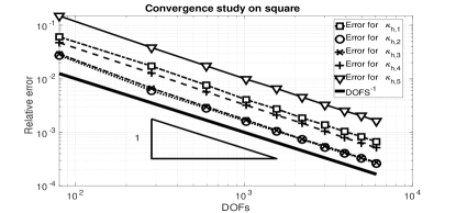
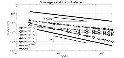
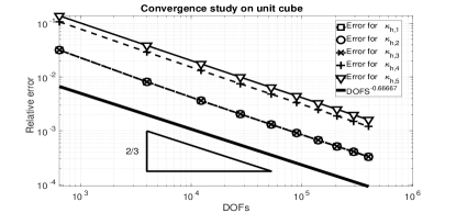
Figure 2: Convergence study for the first 5 eigenvalues of Equation 7 on $\Omega_{1}$ (top-left), $\Omega_{2}$ (to-right), and $\Omega_{3}$ (bottom).

The convergence history of the first 5 eigenvalues of Equation 9 on $\Omega_{1}$ is shown in Figure 2 top-left for the parameters $\mu=10,\,\lambda=1,$ and $\rho=12$. We observe that the discretization method exhibits the expected convergence behaviour as we increase the number of degrees of freedom. We can see that in all 5 cases the error goes down with a similar rate.

For our second example on the L-shaped domain $\Omega_{2}$, we set the parameters $\mu=\lambda=\rho=1$. As expected, the rate of convergence reflects the poor regularity of some eigenfunctions. However, as for other elliptic operators, it seems that some eigenfunctions do not capture the corner singularity at the origin. This is the case for $\kappa_{h,5}$ (Figure 2 bottom). We see that the relative error for this eigenvalues decays as DOFs^-1, suggesting that its corresponding eigenfunctions belong to ${\bf H}^{2}(\Omega_{2})$.

In the last example, we consider the unit cube $\Omega_{3}$ with parameters $\mu=10$, $\lambda=1$, and $\rho=12$. Figure 2 (top right) shows the convergence history of the first five Jones eigenvalues on $\Omega_{3}$. We notice that computed eigenvalues converge at the predicted rate as the triangulation gets refined.

5.2 An example of variable density

Jones modes also can be found when the material density $\rho$ varies. As an example, we consider the unit square $\Omega_{1}$ with a variable density $\rho(x,y)=12|x-0.3||y-0.25|$ and Lamé parameters $\mu=\lambda=1$. The rate of convergence of the first five Jones eigenvalues is shown in Figure 3 top. We see that the error of the computed eigenvalues decays at the same rate as for the case with constant density. The two eigenfunctions shown in Figure 3 middle and bottom correspond to distinct eigenvalues; the weighted ${\bf L}^{2}_{\rho}$-inner product of these eigenfunctions is zero as discussed in subsection 3.3.

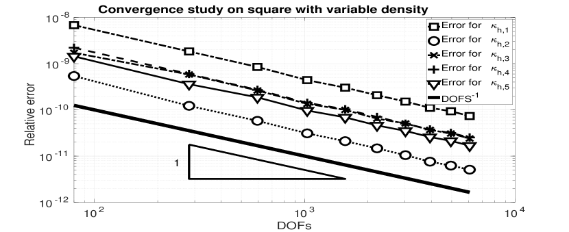
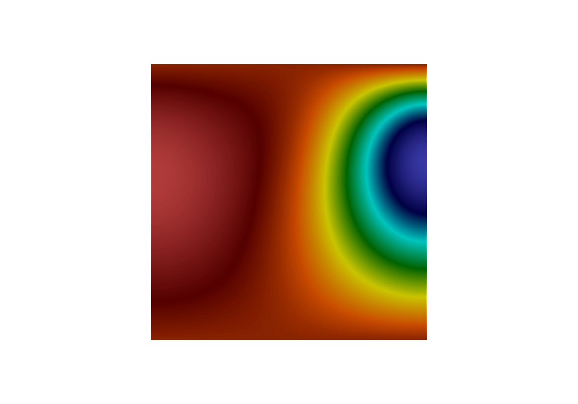
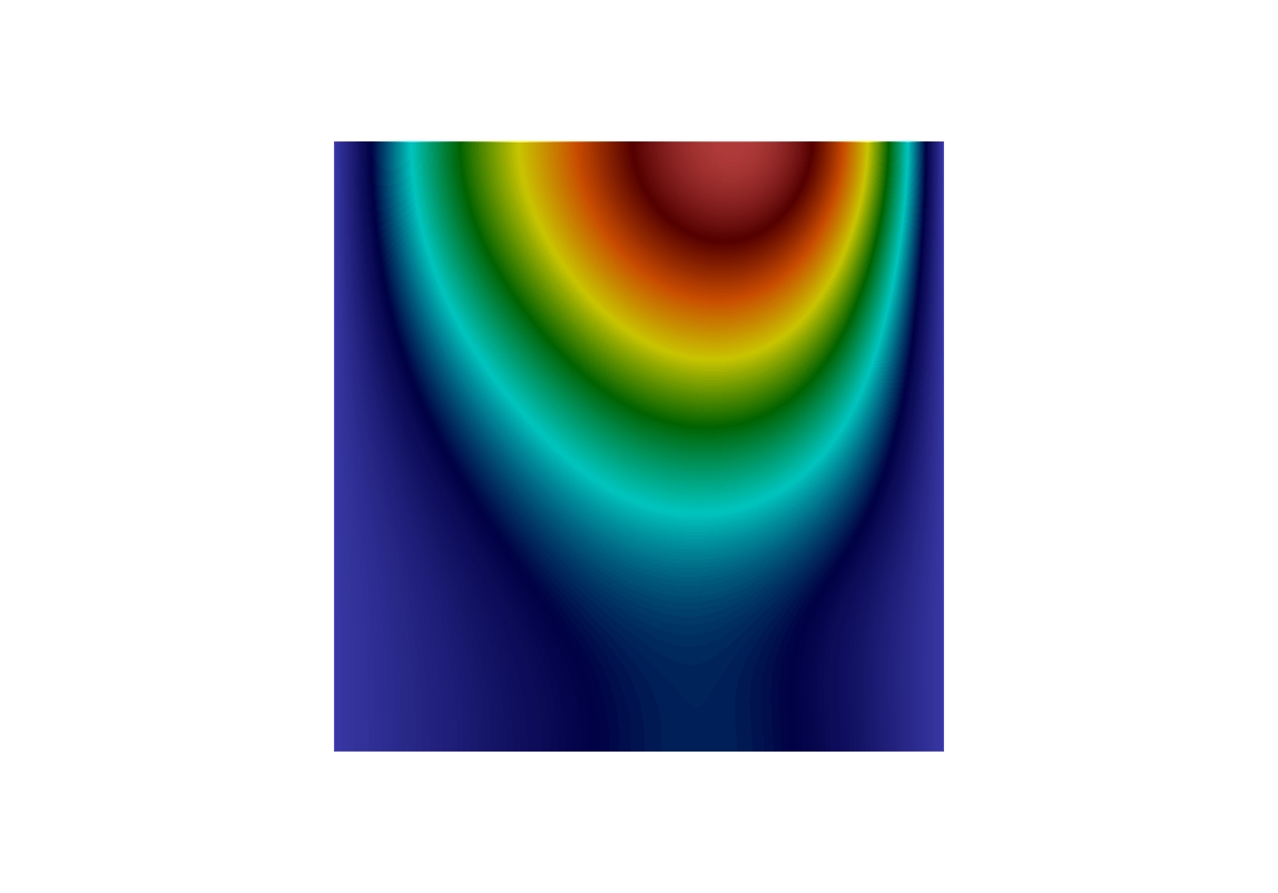
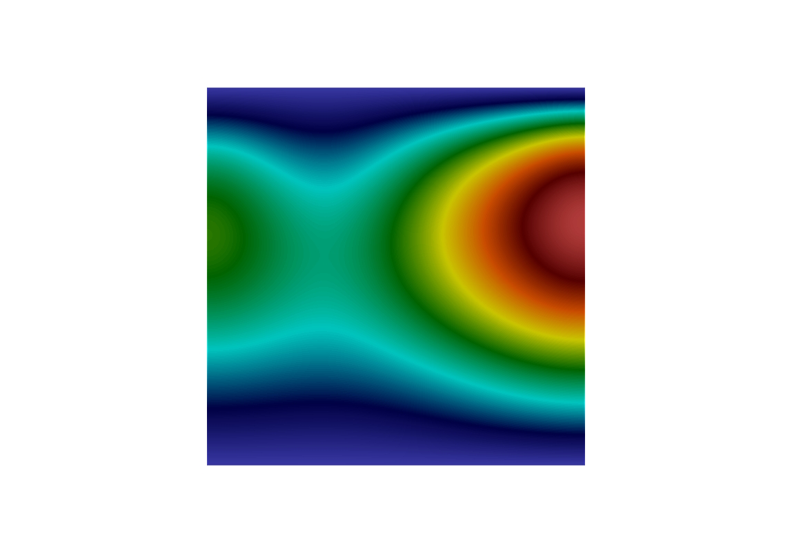
Figure 3: Convergence study (top) of the first 5 Jones on the unit square $\Omega_{1}$ with variable density $\rho(x,y)$. The figures in the middle and bottem represent the x-component (left) and y-component (right) of the Jones eigenmodes associated with $\kappa_{1,h}$ and $\kappa_{2,h}$.

5.3 Jones modes on a disk

We next present numerical results demonstrating conforming discretizations of both the primal formulation Equation 9 and the mixed formulation Equation 29 on the disk, where we have used regular triangles. We consider the unit disk $\Omega_{4}:=B(0,1)$ centered at the origin, with parameters $\mu=1$, $\lambda=1$, and $\rho=1$. As discussed in subsection 3.2, an eigenmode associated to the eigenvalue $\kappa_{1}=0$ is added on the circle (2D case) as a consequence of the symmetry of the domain and the condition on the normal trace of the displacement on the boundary. Figure 4 shows the eigenfunction ${\bf u}_{1}$ associated to $\kappa_{1}$. We can see that this displacement is a rigid mode with a pure tangential displacement towards the boundary.

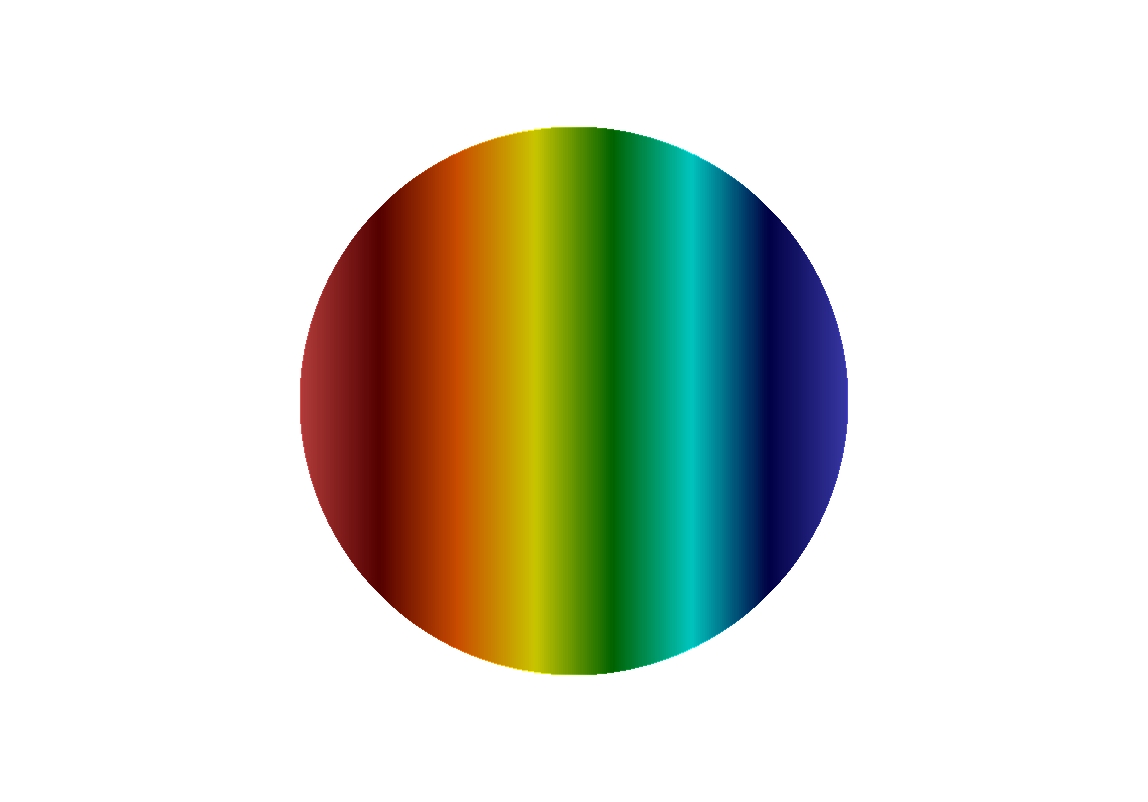
Figure 4: $x$-component (left) and $y$-component (right) of the eigenfunction ${\bf u}_{h,1}$ on the unit disk associated to the eigenvalue $\kappa_{1}=0$. The computations are performed on a grid comprising of triangles.

In Table 1-Table 4, we present the first 5 Jones eigenmodes, computed on the same meshes (over 5 levels of refinement). We observe that the computed spectrum using the primal formulation Table 1-Table 2 misses the first three Jones eigenvalues that the mixed formulation approximates Table 3-Table 4. The mixed formulation accurately captures these modes and, in particular, captures the shifted zero eigenvalue that is added to the spectrum when an axisymmetric domain is considered.

The convergence history of the first five eigenvalues on the circle is shown for a ${\bf P}_{2}-P_{2}$-conforming discrete formulation of Equation 29, with predicted rate of convergence of $h^{2}=$DOFs^-1. The decay for $\kappa_{h,1}$ is of the order of the tolerance we set in the eigenvalue solver. This comes from the fact that $\kappa_{h,1}$ approximates the zero eigenvalue.

DOFs	$\kappa_{1,h}$	$\kappa_{2,h}$	$\kappa_{3,h}$	$\kappa_{4,h}$	$\kappa_{5,h}$
15972	12.32475648	12.32477023	15.6907989	28.29273062	28.29380655
21488	12.32412585	12.32414851	15.68856957	28.28731457	28.28944094
28120	12.32366488	12.32368938	15.68708044	28.28443298	28.28511814
36140	12.32329776	12.32330826	15.68588773	28.28155673	28.28226112
65637	12.32312009	12.32313548	15.68522911	28.28039584	28.28075982

Table 1: First five (shifted) Jones eigenvalues on the unit circle for five levels of refinement, using the P1 conforming scheme (vectorial Lagrange elements) of the primal formulation.

DOFs	$\kappa_{1,h}$	$\kappa_{2,h}$	$\kappa_{3,h}$	$\kappa_{4,h}$	$\kappa_{5,h}$
63282	12.31982312	12.3198605	15.60885775	28.27462732	28.27464639
85246	12.31995092	12.32000357	15.61697078	28.27415568	28.27415894
111674	12.31996175	12.3200125	15.62039435	28.27382317	28.27384615
143654	12.3202651	12.32030354	15.62961012	28.27365126	28.27366316
261039	12.32050245	12.32052281	15.63657853	28.27352834	28.27353722

Table 2: First five (shifted) Jones eigenvalues on the unit circle for five levels of refinement, using the P2 conforming scheme (vectorial Lagrange elements) of the primal formulation.

DOFs	$\kappa_{1,h}$	$\kappa_{2,h}$	$\kappa_{3,h}$	$\kappa_{4,h}$	$\kappa_{5,h}$
23958	1.000000000	6.189626972	6.189643368	13.15499546	13.15505685
32232	1.000000000	6.189248857	6.189257759	13.15390925	13.15400431
42180	1.000000000	6.188970148	6.188978719	13.15310588	13.1531842
54210	1.000000000	6.188735065	6.188747593	13.15246565	13.15249264
65637	1.000000000	6.188634352	6.188638195	13.15215436	13.15220753

Table 3: First five (shifted) Jones eigenvalues on the unit circle for ten different levels of refinement, using a P1-P1 scheme of the mixed formulation.

DOFs	$\kappa_{1,h}$	$\kappa_{2,h}$	$\kappa_{3,h}$	$\kappa_{4,h}$	$\kappa_{5,h}$
94923	1.000000000	6.188425852	6.188425903	13.15133728	13.15133729
127869	1.000000000	6.18832008	6.188320227	13.15110141	13.15110143
167511	1.000000000	6.188251842	6.188251917	13.15094836	13.15094836
215481	1.000000000	6.188205638	6.188205663	13.15084343	13.15084343
261039	1.000000000	6.188172645	6.188172683	13.15076839	13.15076839

Table 4: First five (shifted) Jones eigenvalues on the unit circle for ten different levels of refinement, using a P2-P2 scheme of the mixed formulation.

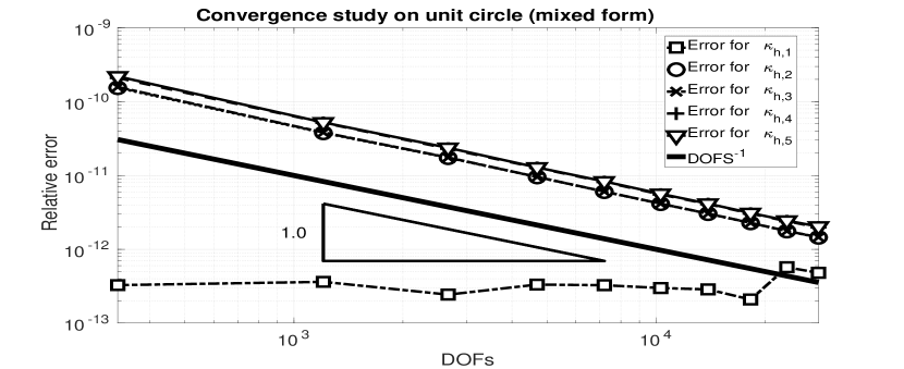
Figure 5: Convergence study for the first 5 eigenvalues of Equation 7 on the unit circle using the mixed formulation with quadratic elements. The approximated eigenvalue $\kappa_{h,1}$ corresponds to the eigenvalue 1.0 in the shifted formulation of Equation 29.

5.4 Shear and compression modes of Jones eigenpairs

We end this section by using the discrete formulation in Equation 23 to compute Jones modes on some geometries, to explore the dependence of the spectrum on domain shape and the Lamé parameters. We also report the $L^{2}$-norm of the divergence and rotational of the computed fields. In simple shapes, as the rectangle, the Jones modes can be readily identified as pure $s$- or $p$- modes. The eigenvalues can also have multiplicity, and the eigenspaces may include eigenmodes of both types. This points to the need for care with resolving eigenmodes, as with any problem involving multiple eigenvalues or clusters of these.

As found in section 3, the Jones eigenvalue problem on Lipschitz domains possesses a countable set of eigenvalues $w_{m\ell}^{2}$, $m,\ell=0,1,2,\ldots$. For the sake of presentation, we set $\nu_{j}=w^{2}_{m\ell}$, with $j=j(m,\ell)\in\mathbb{N}_{0}$, such that $\nu_{j}\leq\nu_{j+1}$, for all $j\in\mathbb{N}_{0}$.

In subsection 2.3, we showed that eigenpairs given by Equation 5 and Equation 6 are part of the spectrum of the Jones eigenproblem on a rectangle. By changing the Lamé parameters, one expects to change not only the eigenvalues, but potentially also the geometric multiplicity of eigenspaces. An example of this behaviour can be seen in Table 5 and Table 6 where we show the first seven approximated Jones eigenpairs on the unit square with parameters $\mu=\rho=1$, and $\lambda\in\{1,2\}$.

$j$	$\nu_{j}$	$\nu_{j}/\pi^{2}$	$\|{\rm div}\,{\bf u}\|_{0}^{2}$	$\|{\rm curl}\,{\bf u}\|_{0}^{2}$	$x-$component	$y-$component
1	19.74	2.000	5.048e-08	19.72
2	29.61	3.000	9.870	0.000188
3	29.61	3.000	9.870	0.0001293
4	49.35	5.000	7.168e-07	49.22
5	49.35	5.000	8.863e-07	49.25
6	59.22	6.000	19.74	0.0005061
7	78.96	8.000	2.979e-06	78.78

Table 5: First 7 eigemodes on unit square with parameters $\mu=\lambda=\rho=1$. $\nu_{2}=\nu_{3}$, and the corresponding eigenspace has pure $p$ modes. Also, $\nu_{4}=\nu_{5}$, and the corresponding eigenspace has pure $s$ modes.

$j$	$\nu_{j}$	$\nu_{j}/\pi^{2}$	$\|{\rm div}\,{\bf u}\|_{0}^{2}$	$\|{\rm curl}\,{\bf u}\|_{0}^{2}$	$x-$component	$y-$component
1	19.74	2.000	5.048e-08	19.72
2	39.48	4.000	9.870	0.000188
3	39.48	4.000	9.870	0.0001294
4	49.35	5.000	6.414e-07	49.22
5	49.35	5.000	8.263e-07	49.25
6	78.96	8.000	19.74	0.0005061
7	78.96	8.000	2.742e-06	78.78

Table 6: First 7 eigenmodes on unit square with parameters $\mu=\rho=1,\lambda=2$. Again, $\nu_{2}=\nu_{3}$, and the corresponding eigenspace has pure $p$ modes; $\nu_{4}=\nu_{5}$, and the corresponding eigenspace has pure $s-$ modes. Note that the eigenspace corresponding to $\nu_{6}$ has an $s$ mode as well as a p-mode, in contrast to Table 5.

From the analytic expressions Equation 6 and Equation 5 for the rectangle, it is clear that by changing the Lamé parameters one can change the multiplicity as well as the composition of eigenspaces. For example, the first eigenmode on a rectangle $[0,1]\times[0,2]$ with $\mu=\lambda=\rho=1$ is a pure $p$ mode; changing $\lambda$ to 10 will make the first eigenmode be a pure $s$ mode.

For shapes other than rectangles, the eigenmodes do not need to be pure $s$ or pure $p$ waves. This points out the fact that the shape of the boundary is an important factor in this problem. The L-shaped domain discussed in the convergence studies is an example of such a domain: due to the re-entrant corner (see Table 7), the eigenmodes are neither pure shear nor pure compression modes. The same can be observed on the isosceles triangle of vertices $(0,0),\,(2,0)$ and $(0,1)$, where none of the eigenfunctions seem to be divergence or curl free (see Table 8).

$j$	$\nu_{j}$	$\nu_{j}/\pi^{2}$	$\|{\rm div}\,{\bf u}\|_{0}^{2}$	$\|{\rm curl}\,{\bf u}\|_{0}^{2}$	$x-$component	$y-$component
1	0.08848	0.008965	0.01531	5.013
2	1.285	0.1302	0.1411	5.273
3	3.8100	0.3861	0.2903	15.43
4	5.1300	0.5197	0.4458	8.277

Table 7: L-shaped domain with parameters $\mu=\lambda=\rho=1$.

$j$	$\nu_{j}$	$\nu_{j}/\pi^{2}$	$\|{\rm div}\,{\bf u}\|_{0}^{2}$	$\|{\rm curl}\,{\bf u}\|_{0}^{2}$	$x-$component	$y-$component
1	4.6563	0.4718	0.7007	24.36
2	8.3125	0.8422	0.4333	14.42
3	11.84674	1.200	2.527	4.15
4	21.0647	2.134	1.640	75.96

Table 8: Isosceles triangle of vertices $(0,0)$, $(2,0)$ and $(0,1)$ with parameters $\lambda=\mu=\rho=1$.

Conclusions

In this work we demonstrated the existence of Jones modes on Lipschitz domains. The spectrum of the Jones eigenproblem (cf. Equation 4) depends heavily on the shape of the domain under consideration (as shown in section 3).

Axisymmetric domains such as bodies of revolution, spheres or disks present more challenges for computation compared to polygonal domains. Concretely, there are two issues in these cases: the presence of a zero eigenvalue, and the discretization of the boundary curve. The former issue is handled by using a shift. The effect of the discretization of the smooth boundary by a polygonal one is more profound. As we saw in the computations for the disk, the primal formulation did not capture the same part of the spectrum. This phenomenon was also found to hold for other smooth domains, such as ellipses.

We believe the reason for this phenomenon is the interplay between the imposition of the constraint on $\mathbf{u\cdot n}$, and the fact that the boundary is being approximated by piecewise linear polynomials. We expect curvilinear elements which are boundary-conforming should ameliorate this problem, and a careful investigation of this is ongoing work.

Acknowledgements

Sebastián Domínguez thanks the support of CONICYT-Chile, through Becas Chile. Nilima Nigam gratefully thanks the financial support of the National Sciences and Engineering Research Council of Canada (NSERC) Discovery Grants and the hospitality of the Institute for Mathematics and its Applications, Minneapolis. The research of Jiguang Sun was partially supported by NSF grant DMS-1521555. The authors are grateful to the anonymous referees for their helpful comments.

This paper is dedicated to George C. Hsiao, Gabriel Gatica and Francisco-Javier Sayas González (Pancho) on the occassion of their 85th, 60th and 50th birthdays respectively. Initial ideas for this work were discussed at length with Pancho. His friendship, intellectual courage and mathematical talent will be deeply missed.

References

- [1] I. Azpiroz. Contribution à la Résolution Numérique de Problm̀es Inverses de Diffraction Élasto-acoustique. PhD thesis, 2018. Thèse de doctorat dirigée par H. Barucq, J. Diaz et R. Djellouli, Mathèmatiques Appliquèes Pau 2018.
- [2] I. Babuska and J. Osborn. Eigenvalue problems. Handbook of Numerical Analysis, 2:641–787, 12 1991.
- [3] H. Barucq, R. Djellouli, and E. Estecahandy. On the existence and the uniqueness of the solution of a fluid–structure interaction scattering problem. J. Math. Anal. and Appl., 412(2):571 – 588, 2014.
- [4] S. Bauer and D. Pauly. On Korn’s first inequality for tangential or normal boundary conditions with explicit constants. Math. Methods Appl. Sci., 39(18):5695–5704, 2016.
- [5] M. Costabel and M. Dauge. Computation of corner singularities in linear elasticity. In Boundary value problems and integral equations in nonsmooth domains (Luminy, 1993), volume 167 of Lecture Notes in Pure and Appl. Math., pages 59–68. Dekker, New York, 1995.
- [6] L. Desvillettes and C. Villani. On a variant of Korn’s inequality arising in statistical mechanics. ESAIM Control Optim. Calc. Var., 8:603–619, 2002. A tribute to J. L. Lions.
- [7] E. Estecahandy. Contribution to the mathematical analysis and to the numerical solution of an inverse elasto-acoustic scattering problem. PhD thesis, Université de Pau et des Pays de l’Adour, September 2013.
- [8] G. N. Gatica, N. Heuer, and S. Meddahi. Coupling of mixed finite element and stabilized boundary element methods for a fluid-solid interaction problem in 3D. Numer. Methods Partial Differential Equations, 30(4):1211–1233, 2014.
- [9] G. N. Gatica, G. C. Hsiao, and S. Meddahi. A residual-based a posteriori error estimator for a two-dimensional fluid–solid interaction problem. Numerische Mathematik, 114(1):63–106, Nov 2009.
- [10] G. N. Gatica, A. Márquez, and S. Meddahi. Analysis of the coupling of BEM, FEM and mixed-FEM for a two-dimensional fluid-solid interaction problem. Appl. Numer. Math., 59(11):2735–2750, 2009.
- [11] P. Grisvard. Singularités en elasticité. Arch. Rational Mech. Anal., 107(2):157–180, 1989.
- [12] T. Hargé. Valeurs propres d’un corps élastique. C. R. Acad. Sci. Paris Sér. I Math., 311(13):857–859, 1990.
- [13] F. Hecht. New development in FreeFem++. J. Numer. Math., 20(3-4):251–266, 2012.
- [14] C. O. Horgan. Korn’s inequalities and their applications in continuum mechanics. SIAM Rev., 37(4):491–511, 1995.
- [15] G. C. Hsiao, R. E. Kleinman, and G. F. Roach. Weak solutions of fluid-solid interaction problems. Math. Nachr., 218:139–163, 2000.
- [16] G. C. Hsiao and N. Nigam. A transmission problem for fluid-structure interaction in the exterior of a thin domain. Adv. Differential Equations, 8(11):1281–1318, 2003.
- [17] G. C. Hsiao, T. Sánchez-Vizuet, and F.-J. Sayas. Boundary and coupled boundary-finite element methods for transient wave-structure interaction. IMA J. Numer. Anal., 37(1):237–265, 2017.
- [18] T. Huttunen, J. P. Kaipio, and P. Monk. An ultra-weak method for acoustic fluid-solid interaction. J. Comput. Appl. Math., 213(1):166–185, 2008.
- [19] D. S. Jones. Low-frequency scattering by a body in lubricated contact. Quart. J. Mech. Appl. Math., 36(1):111–138, 1983.
- [20] R. J. Knops and L. E. Payne. Uniqueness theorems in linear elasticity. Springer-Verlag, New York-Berlin, 1971. Springer Tracts in Natural Philosophy, Vol. 19.
- [21] H. Lamb. On the Vibrations of an Elastic Sphere. Proc. Lond. Math. Soc., 13:189–212, 1881/82.
- [22] C. J. Luke and P. A. Martin. Fluid-solid interaction: acoustic scattering by a smooth elastic obstacle. SIAM J. Appl. Math., 55(4):904–922, 1995.
- [23] P. A. Martin. Shear-wave resonances in a fluid-solid-solid layered structure. Wave Motion, 51(7):1161–1169, 2014.
- [24] S. Meddahi, D. Mora, and R. Rodríguez. Finite element spectral analysis for the mixed formulation of the elasticity equations. SIAM J. Numer. Anal., 51(2):1041–1063, 2013.
- [25] S. Meddahi and F.-J. Sayas. Analysis of a new BEM-FEM coupling for two-dimensional fluid-solid interaction. Numer. Methods Partial Differential Equations, 21(6):1017–1042, 2005.
- [26] D. Natroshvili, G. Sadunishvili, and I. Sigua. Some remarks concerning Jones eigenfrequencies and Jones modes. Georgian Math. J., 12(2):337–348, 2005.
- [27] S. Nicaise. About the Lamé system in a polygonal or a polyhedral domain and a coupled problem between the Lamé system and the plate equation. I. Regularity of the solutions. Ann. Scuola Norm. Sup. Pisa Cl. Sci. (4), 19(3):327–361, 1992.
- [28] A. Rössle. Corner singularities and regularity of weak solutions for the two-dimensional Lamé equations on domains with angular corners. J. Elasticity, 60(1):57–75, 2000.