Efficient ConvNets for Analog Arrays

Abstract

Analog arrays are a promising upcoming hardware technology with the potential to drastically speed up deep learning. Their main advantage is that they compute matrix-vector products in constant time, irrespective of the size of the matrix. However, early convolution layers in ConvNets map very unfavorably onto analog arrays, because kernel matrices are typically small and the constant time operation needs to be sequentially iterated a large number of times, reducing the speed up advantage for ConvNets. Here, we propose to replicate the kernel matrix of a convolution layer on distinct analog arrays, and randomly divide parts of the compute among them, so that multiple kernel matrices are trained in parallel. With this modification, analog arrays execute ConvNets with an acceleration factor that is proportional to the number of kernel matrices used per layer (here tested 16-128). Despite having more free parameters, we show analytically and in numerical experiments that this convolution architecture is self-regularizing and implicitly learns similar filters across arrays. We also report superior performance on a number of datasets and increased robustness to adversarial attacks. Our investigation suggests to revise the notion that mixed analog-digital hardware is not suitable for ConvNets.

1 Introduction

Training deep networks is notoriously computationally intensive. The popularity of ConvNets is largely due to the reduced computational burden they allow thanks to their parsimonious number of free parameters (as compared to fully connected networks), and their favorable mapping on existing graphic processing units (GPUs, [1]).

Recently, speedup strategies of the matrix multiply-and-accumulate (MAC) operation (the computational workhorse of deep learning) based on mixed analog-digital approaches has been gaining increasing attention. Analog arrays of non-volatile memory provide an in-memory compute solution for deep learning that keeps the weights stationary [2, 3]. As a result, the forward, backward and update steps of back-propagation algorithms can be performed with significantly reduced data movement. In general, these analog arrays rely on the idea of implementing matrix-vector multiplications on an array of analog devices by exploiting their Ohmic properties, resulting in a one-step constant time operation, i.e. with execution time independent of the matrix size (up to size limitations due to the device technology) [4].

Matrix-matrix multiplications can harness this time advantage from analog arrays, but since they are implemented as a sequence of matrix-vector products, their execution time is proportional to the number of such products. In other words, the time required to multiply a matrix on an analog array of size $n_{o}\times n_{s}$ with an input matrix of size $n_{s}\times n_{p}$ is not proportional to the overall amount of compute ($\propto n_{o}n_{s}{n_{p}}$, as for conventional hardware [5]), but instead only scales linearly with the number of columns of the input matrix ${n_{p}}$ and is invariant with respect to the size of the matrix stored on the analog array ($n_{o}\times n_{s}$).

These considerations indicate that ConvNets do not map favorably onto analog arrays [6], as becomes clear when one formulates the convolution operation in terms of a matrix-matrix product (see Sec. 2 for a detailed derivation). It turns out that kernel matrices (obtained by flattening and stacking convolution filters), are typically small, corresponding to a small size of the analog $n_{o}\times n_{s}$-array. More crucially, matrix-vector products need to be iterated ${n_{p}}$ times (the number of image patches), which is proportional to the total number of pixels in the input image and can thus be very large, particularly for early conv layers.

A common strategy to speed up training is to use data parallelism, where updates over large batches of data are computed in parallel on independent computing nodes and then averaged (e.g.[7]). However, this is not a practical solution to speed up training on analog arrays, since weight updates are computed only implicitly on stationary weights in non-volatile memory and are thus not directly accessible for averaging [4].

Here, we propose a simple solution to accelerate ConvNets on analog arrays, which we call RAPA Convolution (for Replicated Arrays with Permuted Assignment). The main idea is to use model parallelism to reduce the overall computation time on analog arrays (but not the amount of computation, as done e.g. in [8]). Concretely, we propose to replicate the kernel matrix onto $n_{t}$ separate analog arrays (“tiles”), and to distribute the compute equally among the tiles (see Fig. 1). When this architecture proposed for analog arrays is simulated on conventional hardware (as we do here), it is equivalent to learning multiple kernel matrices independently for individual conv layer. Thus, output pixels of the same image plane will be in general convolved with different filters. Note that we do not explicitly force the kernel matrices to be identical, which would recover the original convolution operation.

In this study, we simulate the RAPA ConvNet in order to validate the effectiveness of different ways to distribute the compute among the tiles and show that it is possible to achieve superior performance to conventional ConvNets with the same kernel matrix sizes. We further prove analytically in a simplified model that for a random assignment of compute to tiles, our architecture is indeed implicitly regularized, such that tiles tend to learn similar kernel matrices. Finally, we find that the RAPA ConvNet is actually more robust to white-box adversarial attacks, since random assignment acts as a “confidence stabilization” mechanism that tends to balance overconfident predictions.

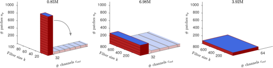
Figure 1: The amount of compute for the example ConvNet (respective for the 3 layers). Blue areas ($k\times c_{\text{out}}$) indicate the size of the kernel matrices. Computing time for analog arrays is proportional only to ${n_{p}}$ and peaks at the first layer, while the amount of compute is $O({n_{p}}kc_{\text{out}})$ (the volume of the red cuboid; MACs in titles) and peaks at the second layer. For each layer, our approach distributes the compute onto multiple replica of the kernel matrix residing on distinct arrays (“tiles”), indicated as tilings of the red cuboids into $n_{t}=(16,4,1)$ small boxes, respectively. Since tiles are trained independently and in parallel, the compute time on analog arrays effectively becomes constant across layers (same height across layers; note, however, that the number of output channels of the convolution does not change). Our tiling schemes refer to the way individual image patches are assigned to the tiles.

2 Convolution with replicated kernel matrices

Following common practice (e.g. [1]), the convolution of a filter of size $k_{h}\times k_{w}$ over an input image of size $h\times w\times c_{\text{in}}$ can be formulated as a matrix-matrix multiplication between an ${n_{p}}\times k$ im2col matrix $I$, constructed by stacking all ${n_{p}}$ (typically overlapping) image patches $\mathbf{b}_{i}$ of size $k_{h}\times k_{w}\times c_{\text{in}}$ in rows of length $k=k_{h}k_{w}c_{\text{in}}$. We can then write $I=\left(\mathbf{b}_{1},\ldots,\mathbf{b}_{n_{p}}\right)^{T}\equiv\left(\mathbf{b}^{T}_{i}\right)_{i\in\{1,\ldots,{n_{p}}\}}$. The matrix $I$ is then multiplied by the $k\times c_{\text{out}}$ kernel matrix $K$, where $c_{\text{out}}$ is the number of output channels (i.e. the number of filters). The result $M=IK$ is of size ${n_{p}}\times c_{\text{out}}$, and is finally reshaped to a tensor with size $\tilde{h}\times\tilde{w}\times c_{\text{out}}$, to reflect the original image content.

In most ConvNets, conv layers are alternated with some form of pooling layers, that reduce the spatial size typically by a factor of 2 (the pool stride) [9]. Thus, for the next convolutional layer, ${n_{p}}$ is reduced by a factor of 4 (square of the pool stride). On the other hand, because output channels become the input channels to the following layer, the size of $K$ changes as well (see Fig. 1).

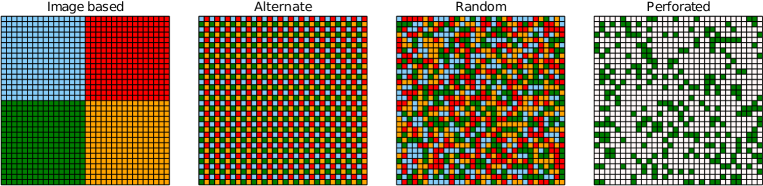
Figure 2: Illustrated is the output of a conv layer for different tiling schemes ($n_{t}=4$, $c_{\text{out}}=1$). Each output pixel might be computed with a kernel matrix from a different array tile (colors; white means zeros).

Our approach to parallelize the compute on analog arrays consists in using $n_{t}$ kernel matrices $K_{j}$ instead of just one $K$ for a given conv layer, and distributing the patches $\mathbf{b}_{i}$ equally among them, so that at any given time $n_{t}$ matrix-vector products can be processed in parallel. Each of the ${n_{p}}$ patches is assigned to exactly one subset $S_{j}\subset\{1,\ldots,{n_{p}}\}$ (all of roughly equal size, $|S_{j}|\approx{n_{p}}/n_{t}$), and the individual array tiles effectively compute the sub-matrices $M_{j}=I_{j}K_{j}=\left(\mathbf{b}^{T}_{l}\right)_{l\in S_{j}}K_{j}$. How the image patches are divided into the subsets $S_{j}$ is what we call “tiling scheme” (see below).

The final result is then obtained by re-ordering the rows according to their original index. In summary, with $s_{l}=j$ if $l\in S_{j}$, we can write $M_{\text{tiled}}=\left(\mathbf{b}^{T}_{l}K_{s_{l}}\right)_{l\in\{1,\ldots,{n_{p}}\}}$. Note that if all $K_{j}$ are identical, the tiled convolution trivially recovers the original convolution. If we assume that each kernel matrix $K_{j}$ resides on a separate analog array tile, and all resulting $I_{j}K_{j}$ operations can be computed in parallel, the overall computation is sped up by a factor of $n_{t}$ (neglecting the effort of the assignment, since that can be done efficiently on the digital side of the mixed analog-digital system).

However, if all $K_{j}$ are learned independently and without explicit synchronization (a prerequisite for embarrassingly parallel execution) filters corresponding to the same output channel might in general be non-identical, which implies that $M_{\text{tiled}}\neq M$. Thus, learning all $K_{j}$ in parallel might negatively impact accuracy. In the following, we test how different tiling schemes affect the overall accuracy. We use the following schemes (compare to Fig. 2).

Image-based tiling

This tiling scheme consists in collecting all patches that contain pixels from a particular image region into a common subset $S_{j}$. If the image is a square with sides of length $n$ and the number of tiles $n_{t}$ is a square number, $n_{t}=q^{2}$, the patch $\mathbf{b}_{i}$ centered at pixel position $(x_{i},y_{i})$ with $x_{i},y_{i}\in\{0,\ldots,n-1\}$ is assigned to the subset $S_{s_{i}}$, with $s_{i}=\left\lfloor\frac{qx_{i}}{n}\right\rfloor+q\left\lfloor\frac{qy_{i}}{n}\right\rfloor+1$. Note that image patches at the border will generally contain pixels from the neighboring regions. We thus call this scheme “image w/overlap”. Alternatively, the pixels from other regions can be set to zero (as if padded in case of separate sub-images), and we call this scheme “image w/pad”.

Alternate tiling

If the image is again a square and $n_{t}=q^{2}$, one could put image patches that are neighboring to each other into different subsets, so that neighboring image patches are assigned to alternate tiles. Specifically, $s_{i}=(x_{i}\mod q)+q\;(y_{i}\mod q)+1$. This tiling is similar to the “tiled convolution” approach suggested by [10] as a way to improve the learning of larger rotational and translational invariances within one convolutional layer.

Random tiling

An alternative way of distributing ${n_{p}}$ image patches onto $n_{t}$ kernel matrices, is to let the $S_{j}$ be a random partition of the set $\{1,\ldots,{n_{p}}\}$, with each of the $S_{j}$ having (roughly) the same size. We investigate two cases: one where the partition is drawn once at the beginning and fixed the remainder (“random fixed”), and the case where we sample a new partition for each train or test image (“random”).

Table 1: Best test (train) error [%] for tiling schemes

Tiling $\backslash$ Data	CIFAR-10	SVHN	CIFAR-100
no tiling	18.85 (2.37)	8.92 (1.96)	47.99 (9.11)
perforated	30.79 (25.93)	13.02 (15.52)	63.44 (50.17)
enlarged	17.75 (0.25)	8.79 (0.71)	46.91 (1.72)
random [fixed]	24.42 (3.86)	11.28 (2.25)	55.50 (23.72)
random	17.67 (5.81)	7.10 (4.13)	48.10 (15.57)
image w/overlap	24.52 (0.99)	10.26 (3.01)	53.22 (18.53)
image w/pad	25.86 (6.53)	11.26 (6.06)	54.24 (28.80)
alternate	21.02 (3.98)	9.22 (2.99)	52.08 (18.83)

Perforated convolution

An alternative way to speed up convolutions, is to simply train a single kernel matrix with only a fraction ${n_{p}}/n_{t}$ of the data [8]. As a result many output pixels will have zero value. Thus, in this scheme we randomly draw a subset $S$ of ${n_{p}}/n_{t}$ indices and set the rows for which $i\notin S$ to $\boldsymbol{0}$, as described for [10]. We resample $S$ for each image during training and use all available image patches during testing. Note that in this scheme only a single kernel matrix is used.

3 Network parameters used in the experiments

We perform a battery of proof of concept experiments using a small standard ConvNet on 3 datasets: CIFAR-10, CIFAR-100 [11], and SVHN [12]. The network  consists of 3 conv layers with kernel size $5\times 5$, and intermediate pooling layers of stride 2. We tried several options for the first 2 pooling layers (see below), whereas the last pooling layer is fixed to an average pooling. Each conv layer is followed by lateral response normalization, and the last conv layer is followed by a fully connected layer. We also use a very small weight decay (0.0001 times the learning rate) and mini-batch of 10, train for $>400$ epochs and report the minimal test and train errors. The learning rate $\lambda$ is annealed in a step-wise manner every 25 epochs with a factor $\lambda_{\gamma}$, and is manually optimized for max-pooling on CIFAR-10, then kept fixed for other datasets and pooling methods. If multiple runs on the datasets were made with different learning rate settings, we report the best test error. We found that $\lambda=0.005$ and $\lambda_{\gamma}=0.5$ for no tiling, and $\lambda=0.05$ and $\lambda_{\gamma}=0.75$ for tiling with $n_{t}=(16,4,1)$ tiles seemed to work best, although different settings, e.g. $\lambda=0.01$ and $\lambda_{\gamma}=0.9$ yield mostly similar results. Note that the number of updates is effectively reduced per array tile, which can be in part compensated by increasing the learning rate. We additionally use a constant “warm up” period of 1 or 5 epochs with a learning rate reduced by a factor of 50.

The output channel setting of the network is $32,32,64$ for the conv layers, respectively. Thus, for CIFAR-10 the network has 79328 weights (including biases) only in the conv layers. For tiling with $n_{t}=(16,4,1)$ tiles, the number of convolutional weights are increased to 192704. To compare this against a network of roughly the same number of weights, we increase the number of channels for the non-tiled network to $54,64,64$, which yields 193032 weights (“enlarged” network). However, note that for this larger network the amount of compute is actually increased, whereas the amount of compute of the tiled network is identical to the original smaller network.

For training we used standard stochastic gradient descent. We use moderate image augmentations (mirroring and brightness changes). All experiments are implemented in Facebook’s Caffe2 framework (using custom C++/CUDA operators, where necessary).

Finally, in addition to the usual pooling methods (max-pooling, average-pooling and stochastic pooling, reviewed e.g. in [9]), we also applied mixed pooling to get the benefits of both max and average pooling. In particular, similar to [13], we use a learnable combination of average and max-pooling, with mixture parameters per channel $\alpha_{k}\in[0,1]$. To enforce these parameter limits, we set $\alpha_{k}\equiv\frac{1}{1+\exp^{\mu\beta_{k}}}$ and train the $\beta_{k}$ with $\mu=10$ fixed. Initial values are $\beta_{k}=2/\mu$ to ensured a bias towards max-pooling, which works best on the datasets used here.

Table 2: Best test (train) error [%] for different pooling methods (CIFAR-10)

Network	no tiling	no tiling, enlarged	random	random	random reduced
Channel	$(32,32,64)$	$(54,64,64)$	$(32,32,64)$	$(32,32,64)$	$(32,32,64)$
$n_{t}$	$(1,1,1)$	$(1,1,1)$	$(16,4,1)$	$(16,4,1)$	$(1,1,1)$
Performance	single test	single test	single test	voting (5)	single test
max pooling	18.93 (0.35)	17.57 (0.04)	17.67 (7.06)	16.89	19.31
average	24.46 (4.29)	23.28 (0.64)	24.32 (7.64)	24.23	24.51
mixed	18.19 (0.42)	17.53 (0.04)	17.37 (6.65)	16.78	18.93
stochastic	20.09 (15.7)	18.39 (11.02)	21.15 (17.32)	18.84	21.19

4 Results

Main experimental results

Our aim here is to systematically quantify the relative impact of our convolutional tiling architecture on performance, not to reach state-of-the-art accuracy on the tested datasets. We therefore examine a relatively small standard ConvNet with 3 conv layers (see Sec. 3).

As described, only the number ${n_{p}}$ of input patches per layer determines the run time on analog arrays. We thus divide the compute of each conv layer onto $n_{t}$ array tiles, so that the number of image patches per tile, ${n_{p}}/n_{t}$, is constant. Since we have ${n_{p}}=(1024,256,64)$, we use $n_{t}=(16,4,1)$ tiles for the 3 conv layers, respectively. Note that this architecture achieves perfect load-balancing, because each tile in the network learns a separate kernel matrix using $64$ image patches per image.

We tested the performance of this setup on the mentioned datasets with and without tiling, and comparing different tiling schemes (see Tab. 1). The main results from these experiments are: (1) “Random” tiling achieves the best performance among all tiling schemes; (2) Across datasets, random tiling actually beats the regular ConvNet with no tiling; (3) Simply subsampling the input images is not sufficient to explain the high performance of random tiling, since the perforated scheme performed poorly.

Filter similarity across tiles

Since replicated kernel matrices are trained independently, it is interesting to examine the similarity of the filters at the end of training. Note that only for identical filters across tiles, the original convolution is recovered.

In general, two main factors tend to implicitly force kernel matrices to become similar during training: (a) input similarity and (b) error-signal similarity across tiles. Indeed, for the random tiling scheme, where the input distribution across tiles is identical on average, different replicated filters might tend to be more similar, but not for other tiling schemes. Indeed, if we quantify the average similarity $S$ of the learned filters across array tiles (computing the average correlation coefficients between all pairs across tiles, averaged over output channels) we find low values for all tiling schemes trained with max-pooling ($S<0.01$), except for the random tiling scheme.

To investigate the effect of the error-signal, we further trained random tiling networks with different pooling methods on CIFAR-10 (see Tab. 2 for performance). For instance, in the case of average pooling, all tiles contributing to pixels in a pooling region will receive the same error signal, whereas for max-pooling only one output pixel per pooling region is selected and used to update the corresponding tile. We find that all pooling methods induce some degree of similarity in case of random tiling ($S>0.1$; see Fig. 3 B for example filters for max pooling). We see the highest similarity for average pooling, where all tiles learn almost identical filters ($S\approx 1$, see Fig. 3 A and C). However, average pooling gives poor performance, suggesting that some diversity among replicated kernel matrices might be advantageous. A good trade-off between similarity and performance can thus be obtained by using a learnable mixture between max and average pooling (Fig. 3A and Tab. 2 mixed pooling).

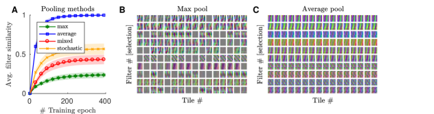
Figure 3: Similarity of learned kernel matrices $K_{j}$ for the first convolution. (A) Similarity of $K_{j}$ for random tiling and different pooling. (B) Selection of 10 out of 32 filters (rows of $K_{j}$; reshaped) for all array tiles for max pooling . (C) Like B but for average pooling.

Comparison with larger model and predictions based on majority vote

Our experiments show that random tiling matches or even outperforms the original network (see Tab. 1 and Tab. 2). However, since replicating kernel matrices onto multiple tiles effectively increases the number of free parameters in the network (by about a factor of 2.5, see Sec. 3), it seems fair to compare the performance of the tiled network with a network with a similar number of free parameters arranged in conventional fashion. When we do that by increasing the number of channels of a non tiled network (which however increases the amount of compute; see Sec. 3), we do indeed find that this enlarged network achieves a performance comparable to the random tiling network (see Tab. 1 and Tab. 2).

It is worth noticing that the performance of the random tiling network in Tab. 1 is obtained by sampling only one random assignment of patches to tiles during test. For each test image, we can instead generate multiple predictions, each generated by a different random assignment, and take as final output the majority vote of all predictions (similarly e.g. to [14]). We test this majority vote over 5 predictions, and see a performance gain of roughly 1% accuracy for the random tiling network, which then outperforms even the enlarged network with adjusted number of parameters (see Tab. 2 second last column). Note, however, that there is no performance gain in case of average pooling, where filters become almost identical (Fig. 3A), indicating an additional benefit of diversity among filter replica at test time.

Reduction of tiled network to the original architecture

It might be problematic for certain applications to retain multiple kernel matrices per conv layer. Thus, one might want to recover the original network, after benefiting from the training speedup of the tiled network. If the filters are very similar (as with average pooling) just taking a kernel matrix of any tile recovers the original convolution and the performance of the original network (see Tab. 2 last column).

One way to reduce the tiled model for mixed or max-pooling, is to select among all replica the filters that most often “wins” the maximum pooling on the training set. These can then be combined to form a single kernel matrix. An alternative simpler way is to just select across tiles the filter with the highest norm, since that indicates a filter that is more often used and updated, and therefore less subject to the weight decay penalty.

We tested this last reduction technique and found that the reduced network’s performance is only slightly worse than the original network with conventional training ($<0.75$% for max/mixed pooling, see Tab. 2), indicating no need for retraining. However, note, that reducing the network to the original architecture also removes the benefits of accelerated run time on analog arrays, the performance gain by majority voting, and the robustness to adversarial attacks (investigated below).

Theoretical analysis: Implicit regularization of random tiling

It is rather intriguing that our random tiling scheme achieves a performance that is comparable or even better than the standard ConvNet. One might have expected that as many as 16 replicated kernel matrices for one conv layer would have incurred overfitting. However, empirically we see that random tiling actually tends to display less overfitting than the standard ConvNet. For example in Tab. 2 (first row) we see that the standard ConvNet (no tiling) achieves a test error of 18.93% with a training error close to zero, while random tiling has a better test error rate of 17.67% with higher training error (7.06%). In this section, we give a formal explanation of this phenomenon and show in a simplified model, a fully-connected logistic regression model, that replicating an architecture’s parameters over multiple “tiles” that are randomly sampled during training acts as an implicit regularization that helps to avoid overfitting.

A logistic regression is a conditional distribution over outputs $y\in\{0,1\}$ given an input vector $\boldsymbol{x}\in\mathbb{R}^{d}$ and a set of paramters $\boldsymbol{\theta}\in\mathbb{R}^{d}$. The exponential family distribution form of the logistic regression is $p(y|\boldsymbol{x},\boldsymbol{\theta})=\exp\left(y~{}\boldsymbol{x}\cdot\boldsymbol{\theta}-A(\boldsymbol{x}\cdot\boldsymbol{\theta})\right)$, where $A(z)\equiv-\log(1-\sigma(z))$ and $\sigma(z)\equiv(1+\exp(-z))^{-1}$ is the logistic function. Note that this expression is equivalent to the more common form $p(y=1|\boldsymbol{x},\boldsymbol{\theta})=\sigma(\boldsymbol{x}\cdot\boldsymbol{\theta})$. Training a logistic regression consists in finding parameters that minimize the empirical negative log-likelihood, $l_{\boldsymbol{x},y}(\boldsymbol{\theta})=-\log p(y|\boldsymbol{x},\boldsymbol{\theta})$, over a given set of $N$ training examples $(\boldsymbol{x}^{i},y^{i})$, resulting in the minimization of the loss: $L(\boldsymbol{\theta})=\sum_{i=1}^{N}l_{\boldsymbol{x}^{i},y^{i}}(\boldsymbol{\theta})$.

We model random tiling by assuming that every parameter $\theta_{l}$ is being replicated over $n_{t}$ tiles. Correspondingly, every time $\theta_{l}$ is being accessed, a parameter $\theta_{l}^{s_{l}}$ with $s_{l}$ randomly sampled in $\{1,\ldots,n_{t}\}$ is retrieved. We write $\boldsymbol{\theta}^{{\boldsymbol{s}}}\equiv(\theta_{l}^{s_{l}})_{l}$ and ${\boldsymbol{s}}\equiv(s_{l})_{l}$. As a result training can be expressed as the minimization of the average loss, $\left\langle L(\boldsymbol{\theta}^{{\boldsymbol{s}}})\right\rangle_{\boldsymbol{s}}=\sum_{i=1}^{N}\left\langle l_{\boldsymbol{x}^{i},y^{i}}(\boldsymbol{\theta}^{{\boldsymbol{s}}})\right\rangle_{\boldsymbol{s}}$, where the angular brackets $\langle\cdot\rangle_{\boldsymbol{s}}$ indicate averaging over the process of randomly sampling every parameter $\theta_{l}$ from a tile $s_{l}$. With the above, we get $\left\langle L(\boldsymbol{\theta}^{{\boldsymbol{s}}})\right\rangle_{\boldsymbol{s}}=-\sum_{i=1}^{N}\left(y^{i}~{}\boldsymbol{x}^{i}\cdot\boldsymbol{\bar{\theta}}-\left\langle A\left(\boldsymbol{x}^{i}\cdot\boldsymbol{\theta}^{{\boldsymbol{s}}}\right)\right\rangle_{\boldsymbol{s}}\right)=L(\boldsymbol{\bar{\theta}})+R(\{\boldsymbol{\theta}^{{\boldsymbol{s}}}\})$, where $\boldsymbol{\bar{\theta}}$ is the vector whose components are the parameters averaged across tiles, i.e. $\bar{\theta}_{l}=\langle\theta_{l}^{s_{l}}\rangle_{\boldsymbol{s}}$, and

$$R(\{\boldsymbol{\theta}^{{\boldsymbol{s}}}\})=\sum_{i=1}^{N}\left(\left\langle A\left(\boldsymbol{x}^{i}\cdot\boldsymbol{\theta}^{{\boldsymbol{s}}}\right)\right\rangle_{\boldsymbol{s}}-A\left(\boldsymbol{x}^{i}\cdot\boldsymbol{\bar{\theta}}\right)\right).$$

The term $R(\{\boldsymbol{\theta}^{{\boldsymbol{s}}}\})$ that falls out of this calculation has the role of a regularizer, since it does not depend on the labels $y^{i}$. In a sense, it acts as an additional cost penalizing the deviations of the replicated parameters $\boldsymbol{\theta}^{{\boldsymbol{s}}}$ from their average value $\boldsymbol{\bar{\theta}}$ across tiles. This tendency of the replicated parameters to move towards the mean counteracts the entropic pressure that training through stochastic gradient descent puts on the replica to move away from each other (see e.g. [15]), therefore reducing the effective number of parameters. This implicit regularization effect explains why, despite the apparent over-parametrization due to replicating the parameters over tiles, our architecture does not seem to overfit more than its standard counterpart. It also explains the tendency of the tiles to synchronize causing the filters to become similar (Fig. 3).

Robustness against adversarial examples

We can gain further intuition on the role of the regularizer $R(\{\boldsymbol{\theta}^{{\boldsymbol{s}}}\})$ by developing its first term as a Taylor series up to second order around $\boldsymbol{x}^{i}\cdot\boldsymbol{\bar{\theta}}$, analogously to what is done in [16, 17]. This results in:

$$R(\{\boldsymbol{\theta}^{{\boldsymbol{s}}}\})\approx\frac{1}{2}\sum_{i=1}^{N}A^{\prime\prime}\left(\boldsymbol{x}^{i}\cdot\boldsymbol{\bar{\theta}}\right)\sum_{l}(x_{l}^{i})^{2}~{}\text{Var}_{\boldsymbol{s}}(\theta_{l}^{s_{l}})=\frac{1}{2}\sum_{i=1}^{N}p_{i}(1-p_{i})\sum_{l}(x_{l}^{i})^{2}~{}\text{Var}_{\boldsymbol{s}}(\theta_{l}^{s_{l}}),$$

where $\text{Var}_{\boldsymbol{s}}(\theta_{l}^{s_{l}})$ is the variance of the parameter $\theta_{l}$ across tiles, and $p_{i}=\sigma\left(\boldsymbol{x}^{i}\cdot\boldsymbol{\bar{\theta}}\right)$ is the predicted probability that $y^{i}=1$ when considering the parameter mean $\boldsymbol{\bar{\theta}}$. This penalty $R(\{\boldsymbol{\theta}^{{\boldsymbol{s}}}\})$ can be interpreted as trying to compensate for high-confidence predictions (for which the term $p_{i}(1-p_{i})$ is small) by diminishing the pressure on $\text{Var}_{\boldsymbol{s}}(\theta_{l}^{s_{l}})$ to be small. As a result, samples $\boldsymbol{x}^{i}$’s for which the prediction will tend to be confident will be multiplied by weights $\theta_{l}$ that will display a relatively large variability across replica, which in turn will tend to reduce the degree of confidence.

This “confidence stabilization” effect raises the intriguing possibility that random tiling mitigates the weaknesses due to a model excessively high prediction confidence. The efficacy of adversarial examples, i.e. samples obtained with small perturbations resulting in intentional high-confidence misclassifications, is such a type of weakness that plagues several machine learning models [18]. Our analysis, suggests that random tiling should help immunize a model against this type of attacks, by preventing the model from being fooled with high confidence.

We verify the theoretical prediction that random tiling increases the robustness to adversarial samples by using the Fast Gradient Sign Method (FSGM) [18] to attack a network trained on CIFAR-10 with max-pooling (see performance results in Tab. 2). In particular, we computed the accuracy drop from all correctly classified images in the test set, due to a perturbation by noise in the direction of the signed error gradient [18] (with strength $\epsilon$). Following [19], we computed the drop in accuracy as a function of the signal-to-noise ratio resulting from adversarial noise (see Fig. 4). At a noise level corresponding to the threshold of human perception, $\epsilon\approx 33$ (according to [19]), we find that random tiling reduces the gap to perfect adversarial robustness by around $41$%. In comparison, other learning methods, such as [19] or enhancing training examples with adversarial gradients [18] reduces the gap on CIFAR-10 by around $6\%$ and $54$%, respectively (using their baseline, compare to [19], Table 1). While the networks used here are not the same as those used in [19], our results still suggest that random tiling significantly improves robustness, with no loss in performance or extra training examples.

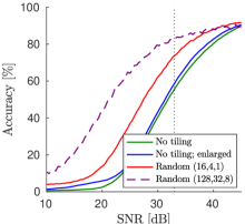
Figure 4: Tiling improves robustness to adversarial examples.

A strategy to further improve robustness is to increase the number of tiles in the random tiling network. If we set $n_{t}=(128,32,8)$ the network still trains fine, reaching a test error of $16.83$% on CIFAR-10, which is similar to the $n_{t}=(16,4,1)$ tiled network (within 500 epochs; max-pool; majority vote of 9 tests; compare to Tab. 2). However, now robustness to adversarial attacks is significantly improved, reaching an accuracy of $83.97$% for $\epsilon\approx 33$ (see Fig. 4; dashed line), which translates to a reduction of the gap to perfect robustness by $64$%. Note that, although the $n_{t}=(128,32,8)$ network has now about $20$ times more convolutional weights than the original non-tiled network, it trains well and does not overfit (training error 15%) and, neglecting peripheral costs and assuming parallel execution of all analog array tiles in a layer, would execute a training epoch $128$ times faster than the original network.

5 Discussion

We here propose a way how to modify ConvNets, so that they map more favorably onto upcoming mixed analog-digital hardware. Interestingly, we find that using multiple independently trained kernel matrices per convolution instead of a single one, and randomly dividing the compute among them, yields no loss in accuracy. Our architecture has the added advantage that, executed on parallel analog arrays, it would in principle run $n_{t}$-times faster than conv layers run on an individual analog array. We show that random assignment regularizes the training, avoiding overfitting, and, additionally, increases the robustness towards adversarial attacks.

We here studied and validated the principles of our architecture in a small standard ConvNet. However, we expect the tiling architecture to be applicable also to larger ConvNets (e.g. [20]), because they generally successively reduce the spatial size with depth through pooling [9] and thus have a similar pattern of the amount of compute per layer as our example network (Fig. 1). For instance, an efficient tiling of the architecture in [20] would be $n_{t}=(17,4,1,1,1)$. This would achieve perfect load-balancing across the 5 conv layers on analog arrays. Note that if set-up in this way, the whole network (including the fully connected layers) can additionally be pipelined across image batches [21], because the duration of computation would be identical for each of the conv layers (irrespective of the different filter sizes and numbers of channels).

There are many different approaches to accelerate deep learning using current hardware [21]. Our approach is motivated by the constraints of mixed-analog digital hardware to emphasize its advantages. In our tiling approach, although the total amount of compute in the network is kept constant (contrary to e.g. methods that perforate the loop [8], or use low-rank approximations or low precision weights, reviewed in [9]), the number of updates per weight is nevertheless reduced, which might generally affect learning curves. Importantly, however, this does not seem to have an impact on the number of training epochs needed to achieve a performance close to the best performance of conventional networks. In fact, the random tiling network (with majority vote) reaches a test error of 19% (mixed pooling, see Tab. 2) after 85 epochs versus 82 for the original network. Admittedly, if one is instead interested in reaching the superior performance of the random tiling network, one would typically need to add additional training time. To what degree the added training time could be reduced by heterogeneous learning rates across the tiled network, is subject of future research.

Finally, another interesting research direction is how the performance of RAPA ConvNets could be further improved by increasing the convolution filter size or the number of filters per layer. Remarkably, this type of modifications, which are generally avoided on GPUs for reasons of efficiency, would not alter the overall run time on upcoming mixed analog-digital hardware technology.

References

- [1] Sharan Chetlur, Cliff Woolley, Philippe Vandermersch, Jonathan Cohen, John Tran, Bryan Catanzaro, and Evan Shelhamer. cudnn: Efficient primitives for deep learning. arXiv preprint arXiv:1410.0759, 2014.
- [2] J Joshua Yang, Dmitri B Strukov, and Duncan R Stewart. Memristive devices for computing. Nature nanotechnology, 8(1):13, 2013.
- [3] Alessandro Fumarola, Pritish Narayanan, Lucas L Sanches, Severin Sidler, Junwoo Jang, Kibong Moon, Robert M Shelby, Hyunsang Hwang, and Geoffrey W Burr. Accelerating machine learning with non-volatile memory: Exploring device and circuit tradeoffs. In Rebooting Computing (ICRC), IEEE International Conference on, pages 1–8. Ieee, 2016.
- [4] Tayfun Gokmen and Yurii Vlasov. Acceleration of deep neural network training with resistive cross-point devices: design considerations. Frontiers in neuroscience, 10:333, 2016.
- [5] Kaiming He and Jian Sun. Convolutional neural networks at constrained time cost. In Computer Vision and Pattern Recognition (CVPR), 2015 IEEE Conference on, pages 5353–5360. IEEE, 2015.
- [6] Tayfun Gokmen, Murat Onen, and Wilfried Haensch. Training deep convolutional neural networks with resistive cross-point devices. Frontiers in neuroscience, 11:538, 2017.
- [7] Yang You, Zhao Zhang, C Hsieh, James Demmel, and Kurt Keutzer. Imagenet training in minutes. CoRR, abs/1709.05011, 2017.
- [8] Mikhail Figurnov, Aizhan Ibraimova, Dmitry P Vetrov, and Pushmeet Kohli. Perforatedcnns: Acceleration through elimination of redundant convolutions. In Advances in Neural Information Processing Systems, pages 947–955, 2016.
- [9] Jiuxiang Gu, Zhenhua Wang, Jason Kuen, Lianyang Ma, Amir Shahroudy, Bing Shuai, Ting Liu, Xingxing Wang, Gang Wang, Jianfei Cai, et al. Recent advances in convolutional neural networks. Pattern Recognition, 2017.
- [10] Jiquan Ngiam, Zhenghao Chen, Daniel Chia, Pang W Koh, Quoc V Le, and Andrew Y Ng. Tiled convolutional neural networks. In Advances in neural information processing systems, pages 1279–1287, 2010.
- [11] Alex Krizhevsky and Geoffrey Hinton. Learning multiple layers of features from tiny images. 2009.
- [12] Yuval Netzer, Tao Wang, Adam Coates, Alessandro Bissacco, Bo Wu, and Andrew Y Ng. Reading digits in natural images with unsupervised feature learning. In NIPS workshop on deep learning and unsupervised feature learning, 2011.
- [13] Dingjun Yu, Hanli Wang, Peiqiu Chen, and Zhihua Wei. Mixed pooling for convolutional neural networks. In International Conference on Rough Sets and Knowledge Technology, pages 364–375. Springer, 2014.
- [14] Benjamin Graham. Fractional max-pooling. arXiv preprint arXiv:1412.6071, 2014.
- [15] Yao Zhang, Andrew M Saxe, Madhu S Advani, and Alpha A Lee. Energy-entropy competition and the effectiveness of stochastic gradient descent in machine learning. arXiv preprint arXiv:1803.01927, 2018.
- [16] Chris M Bishop. Training with noise is equivalent to tikhonov regularization. Neural computation, 7(1):108–116, 1995.
- [17] Stefan Wager, Sida Wang, and Percy S Liang. Dropout training as adaptive regularization. In Advances in neural information processing systems, pages 351–359, 2013.
- [18] Ian J Goodfellow, Jonathon Shlens, and Christian Szegedy. Explaining and harnessing adversarial examples. arXiv preprint arXiv:1412.6572, 2014.
- [19] Moustapha Cisse, Piotr Bojanowski, Edouard Grave, Yann Dauphin, and Nicolas Usunier. Parseval networks: Improving robustness to adversarial examples. In International Conference on Machine Learning, pages 854–863, 2017.
- [20] Alex Krizhevsky, Ilya Sutskever, and Geoffrey E Hinton. Imagenet classification with deep convolutional neural networks. In Advances in neural information processing systems, pages 1097–1105, 2012.
- [21] Tal Ben-Nun and Torsten Hoefler. Demystifying parallel and distributed deep learning: An in-depth concurrency analysis. arXiv preprint arXiv:1802.09941, 2018.