On the Computational Power of Online Gradient Descent

Abstract

We prove that the evolution of weight vectors in online gradient descent can encode arbitrary polynomial-space computations, even in very simple learning settings. Our results imply that, under weak complexity-theoretic assumptions, it is impossible to reason efficiently about the fine-grained behavior of online gradient descent.

1 Introduction

In online convex optimization (OCO), an online algorithm picks a sequence of points $\mathbf{w}^{1},\mathbf{w}^{2},...$ from a compact convex set $\mathcal{K}\subseteq\mathbb{R}^{d}$ while an adversary chooses a sequence $f_{1},f_{2},...$ of convex cost functions (from $\mathcal{K}$ to $\mathbb{R}$). The online algorithm can choose $\mathbf{w}_{t}$ based on the previously-seen $f^{1},...,f^{t-1}$ but not later functions; the adversary can choose $f^{t}$ based on $\mathbf{w}^{1},...,\mathbf{w}^{t}$. The algorithm incurs a cost of $f^{t}(\mathbf{w}^{t})$ at time $t$. Canonically, in a machine learning context, $\mathcal{K}$ is the set of allowable weight vectors or hypotheses (e.g., vectors with bounded $\ell_{2}$-norm), and $f^{t}$ is induced by a data point $\mathbf{x}^{t}$, a label $y^{t}$, and a loss function $\ell$ (e.g., absolute, hinge, or squared loss) via $f^{t}(\mathbf{w}^{t})=\ell(\mathbf{w}^{t},(\mathbf{x}^{t},y^{t}))$.

One of the most well-studied algorithms for OCO is online gradient descent (OGD), which always chooses the point $\mathbf{w}^{t+1}:=\mathbf{w}^{t}-\eta\cdot\nabla f^{t}(\mathbf{w}^{t})$ (Zinkevich, 2003), projecting back to $\mathcal{K}$ if necessary. This algorithm enjoys good guarantees for OCO problems, such as vanishing regret (see e.g. Hazan (2016)).

The main message of this paper is:

• OGD captures arbitrary polynomial-space computations, even in very simple settings.

For example, this result is true for binary classification using soft-margin support vector machines (SVMs) or neural networks with one hidden layer, ReLU activations, and the squared loss function. (For even simpler models, like ordinary linear least squares, such a result appears impossible; see Appendix A.)

A bit more precisely: for every polynomial-space computation, there is a sequence of data points $(\mathbf{x}^{1},y^{1}),\ldots,(\mathbf{x}^{T},y^{T})$ that have polynomial bit complexity such that, if these data points are fed to OGD (specialized to one of the aforementioned settings) in this order over and over again, the consequent sequence of weight vectors simulates the given computation. Figure 1 gives a cartoon view of what such a simulation looks like.

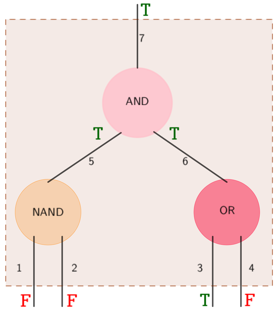
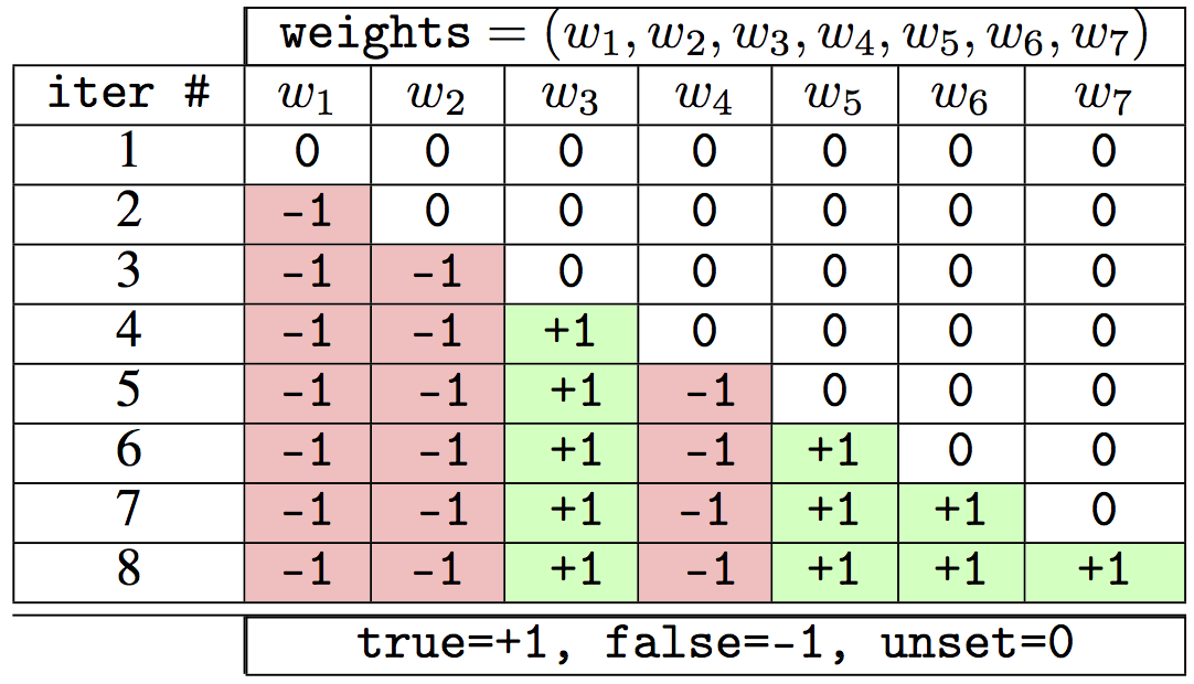
Figure 1: Cartoon view of simulating a computation using a sequence of weight vectors. On the left, the evaluation of a Boolean circuit on a specific input (with “T” and “F” indicating which inputs and gates evaluate to true and false, respectively). On the right, a corresponding sequence of weight vectors (with updates triggered by a carefully chosen data set), with each vector evaluating one more gate of the circuit than the previous one. Weights of $+1,-1$, and $0$ indicate that an input has been assigned true, has been assigned false, or has not yet been assigned a value, respectively.

Our simulation implies that, under weak complexity-theoretic assumptions, it is impossible to reason efficiently about the fine-grained behavior of OGD. For example, the following problem is $\mathbb{PSPACE}$-hard: given a sequence $(\mathbf{x}^{1},y^{1}),\ldots,(\mathbf{x}^{T},y^{T})$ of data points, to be fed into OGD over and over again (in the same order), with initial weights $\mathbf{w}^{1}=\mathbf{0}$, does any weight vector $\mathbf{w}^{t}$ produced by OGD (with soft-margin SVM updates) have a positive first coordinate?

In the case of soft-margin SVMs, for the instances produced by our reduction, the optimal point in hindsight converges over time to a single point $\mathbf{w}^{*}$ (the regularized ERM solution for the initial data set), and the well-known regret guarantees for OGD imply that its iterates grow close to $\mathbf{w}^{*}$ (in objective function value and, by strong convexity, in distance as well). Viewed from afar, OGD is nearly converging; viewed up close, it exhibits astonishing complexity.

Our results have similar implications for a common-in-practice variant of stochastic gradient descent (SGD), where every epoch performs a single pass over the data points, in a fixed but arbitrary order. Our work implies that this variant of SGD can also simulate arbitrary $\mathbb{PSPACE}$ computations (when the data points and their ordering can be chosen adversarially).

1.1 Related Work

There are a number of excellent sources for further background on OCO, OGD, and SVMs; see e.g. Hazan (2016); Shalev-Shwartz and Ben-David (2014). We use only classical concepts from complexity theory, covered e.g. in Sipser (2006).

There is a long history of $\mathbb{PSPACE}$-completeness results for reasoning about iterative algorithms. For example, $\mathbb{PSPACE}$-completeness results were proved for computing the final outcome of local search (Johnson et al., 1988) and other path-following-type algorithms (Goldberg et al., 2013). For a more recent example that concerns finding a limit cycle of certain dynamical systems, see Papadimitriou and Vishnoi (2016).

This paper is most closely related to a line of work showing that certain widely used algorithms inadvertently solve much harder problems than what they were originally designed for. For example, Adler et al. (2014), Disser and Skutella (2015), and Fearnley and Savani (2015) show how to efficiently embed an instance of a hard problem into a linear program so that the trajectory of the simplex method immediately reveals the answer to the instance. Roughgarden and Wang (2016) proved an analogous $\mathbb{PSPACE}$-completeness result for Lloyd’s $k$-means algorithm.

More distantly related are previous works that treat stochastic gradient descent as a dynamical system and then show that the system is complex in some sense. Examples include Van Den Doel and Ascher (2012), who provide empirical evidence of chaotic behavior, and Chaudhari and Soatto (2018), who show that, for DNN training, SGD can converge to stable limit cycles. We are not aware of any previous works that take a computational complexity-based approach to the problem.

2 Preliminaries

2.1 Soft-Margin SVMs

We begin with the following special case of OCO, corresponding to soft-margin support vector machines (SVMs) under a hinge loss. For some fixed regularization parameter $\lambda$, every cost function $f^{t}$ will have the form

$$\ell_{hinge}(\mathbf{w}^{t},(\mathbf{x}^{t},y^{t}))+\tfrac{\lambda}{2}\|\mathbf{w}^{t}\|_{2}^{2}$$

for some data point $\mathbf{x}^{t}\in\mathbb{R}^{d}$ and label $y^{t}\in\{-1,+1\}$, where the hinge loss is defined as $\ell_{hinge}(\mathbf{w}^{t},(\mathbf{x}^{t},y^{t}))=\max\{0,1-y^{t}(\mathbf{w}^{t}\cdot\mathbf{x}^{t})\}$. In this case, the weight updates in OGD have a special form (where $\eta$ is the step size):

$$\mathbf{w}^{t+1}=(1-\lambda\eta)\mathbf{w}^{t}+\eta\cdot\left\{\begin{array}[]{cl}y^{t}(\mathbf{x}^{t})&\text{if $y^{t}(\mathbf{w}^{t}\cdot\mathbf{x}^{t})<1$}\\ 0&\text{if $y^{t}(\mathbf{w}^{t}\cdot\mathbf{x}^{t})>1$.}\end{array}\right.$$

2.2 Complexity Theory Background

A decision problem $L\subseteq\{0,1\}^{*}$ is in the class $\mathbb{PSPACE}$ if and only if there exists a Turing machine $M$ and a polynomial function $p(\cdot)$ such that, for every $n$-bit string $z$, $M$ correctly decides whether or not $z$ is in $L$ while using space at most $p(n)$.

$\mathbb{PSPACE}$ is obviously at least as big as $\mathbb{P}$, the class of polynomial-time-decidable decision problems (it takes $s$ operations to use up $s$ tape cells). It also contains every problem in ${\mathbb{NP}}$ (just try all possible polynomial-length witnesses, reusing space for each computation), $co$-$\mathbb{NP}$ (for the same reason), the entire polynomial hierarchy, and more. A problem $L$ is $\mathbb{PSPACE}$-hard if every problem in $\mathbb{PSPACE}$ polynomial-time reduces to it, and $\mathbb{PSPACE}$-complete if additionally $L$ belongs to $\mathbb{PSPACE}$. While the current state of knowledge does not rule out $\mathbb{P=PSPACE}$ (which would be even more surprising than $\mathbb{P=NP}$), the widespread belief is that $\mathbb{PSPACE}$ contains many problems that are intrinsically computationally difficult (like the aforementioned chess example). Thus a problem that is complete (or hard) for $\mathbb{PSPACE}$ would seem to be very hard indeed.

Our main reduction is from the $\mathcal{C}$-Path problem. In this problem, the input is (an encoding of) a Boolean circuit $\mathcal{C}$ with $n$ inputs, $n$ outputs, and gates of fan-in $2$; and a target $n$-bit string $s^{*}$. The goal is to decide whether or not the repeated application of $\mathcal{C}$ to the all-false string ever produces the output $s^{*}$. This problem is $\mathbb{PSPACE}$-complete (see Adler et al. (2014)), and in this sense every polynomial-space computation is just a thinly disguised instance of $\mathcal{C}$-Path.

3 ${\mathbb{PSPACE}}$-Hardness Reduction

In this section, we present our main reduction from the $\mathcal{C}$-Path problem. Our reduction uses several types of gadgets, which are organized into an API in Subsection 3.2.

The implementation of two gadgets is given in Section 4 and the remaining implementations can be found in Appendix B. After presenting the API, this section concludes by showing how the reduction can be performed using the API.

3.1 Simplifying Assumptions

For this section, we make a couple of simplifying assumptions to showcase the main technical ideas used in our proof. We later show how to extend the proof to remove these assumptions in Section 5. Our simplifying assumptions are:

1. There is no bias term, i.e. $b$ is fixed to $0$.

2. The learning rate $\eta$ is fixed to $1$.

3. The loss function is not regularized, i.e. $\lambda=0$.

3.2 API for Reduction Gadgets

We use a number of gadgets to encode an instance of $\mathcal{C}$-Path into training examples for OGD. The high level plan is to use the weights $\mathbf{w}^{t}$ to encode boolean values in our circuit. A weight of $+1$ will represent a true bit, while a weight of $-1$ will represent a false bit. Additionally, we use a weight of $0$ to represent a bit that we have not yet computed (which we refer to as “unset”). For example, our simplest gadget is reset$\left(i_{1}\right)$, which takes the index of a weight that is set to either +1 or -1, and provides a sequence of training examples that causes that weight to update to 0 (thus unsetting the bit). Our next simplest gadget is not$\left(i_{1}\right)$, which takes the index of a weight that is set to either +1 or -1, and provides a sequence of training examples that causes the weight to update to -1 or +1, respectively (thus setting it to the not of itself). Note that our main reduction does not use the not gadget directly, but it serves as a subgadget for our other gadgets and is also useful for performing other reductions.

It is well known that every $\{\pm 1\}$ Boolean circuit can be efficiently converted into a circuit that only has NAND gates (where the output is $-1$ if both inputs are $+1$, and $+1$ otherwise), and so we focus on such circuits. We would like a gadget that takes two true/false bits and an unset bit and writes the NAND of the first two into the third. Unfortunately, the nature of the weight updates makes it difficult to implement NAND directly. As a result, we instead use two smaller gadgets that can together be used to compute a NAND. The bulk of the work is done by destructive_nand$\left(i_{1},i_{2},i_{3}\right)$, which performs the above but has the unfortunate side-effect of unsetting the first two bits. As a result, we need a way to increase the number of copies we have of a boolean value. The copy$\left(i_{1},i_{2}\right)$ gadget takes a true/false bit and an unset bit and writes the former into the latter. Taken together, we can compute NAND by copying our two bits of interest and then using the copies to compute the NAND.

Our next gadget allows the starting weights $\mathbf{w}^{0}$ to be the all-zeroes vector. The gadget
set_false_if_unset$\left(i_{1}\right)$ takes a weight that may correspond to either a true/false bit or to an unset bit. If the weight is already true/false, it does nothing. Otherwise, it takes the unset bit and writes false into it.

Finally, we have a simple gadget for the purpose of presenting a concrete $\mathbb{PSPACE}$-hard decision problem about the OGD process. The question we aim for is, does any weight vector $\mathbf{w}^{t}$ produced by OGD (with soft-margin SVM updates) have a positive first coordinate? Correspondingly, the set_if_true gadget takes a true/false bit and a zero-weight coordinate (intended to be the first coordinate). If the first bit is true, this gadget gives the zero-weight coordinate a weight of $+1$. If the first bit is false, this gadget leaves the zero-weight coordinate completely untouched, even in intermediate steps between its training examples. This property is not present in the implementation of our other gadgets, so this will be the only gadget that we use to modify the first coordinate.

This API is formally specified in Table 1.

Table 1: Public API

Function	Precondition(s)	Description
reset$\left(i_{1}\right)$	$i_{1}\in\{1,\ldots,d\}$	$w_{i_{1}}\leftarrow 0$
(for implementation, see Table 3)	$w_{i_{1}}\in\{-1,+1\}$
not$\left(i_{1}\right)$	$i_{1}\in\{1,\ldots,d\}$	$w_{i_{1}}\leftarrow\text{NOT}(w_{i_{1}})$
(for implementation, see Table 3)	$w_{i_{1}}\in\{-1,+1\}$
copy$\left(i_{1},i_{2}\right)$	$i_{1},i_{2}\in\{1,\ldots,d\}$	$w_{i_{2}}\leftarrow w_{i_{1}}$
(for implementation, see Table 5)	$w_{i_{1}}\in\{-1,+1\}$
	$w_{i_{2}}=0$
destructive_nand$\left(i_{1},i_{2},i_{3}\right)$	$i_{1},i_{2},i_{3}\in\{1,\ldots,d\}$	$w_{i_{3}}\leftarrow\text{NAND}(w_{i_{1}},w_{i_{2}})$
(for implementation, see Table 6)	$w_{i_{1}}\in\{-1,+1\}$	$w_{i_{1}}\leftarrow 0$
	$w_{i_{2}}\in\{-1,+1\}$	$w_{i_{2}}\leftarrow 0$
	$w_{i_{3}}=0$
set_false_if_unset$\left(i_{1}\right)$	$i_{1}\in\{1,\ldots,d\}$	If $w_{i_{1}}==0$, $w_{i_{1}}\leftarrow-1$
(for implementation, see Table 7)	$w_{i_{1}}\in\{-1,0,+1\}$
copy_if_true$\left(i_{1},i_{2}\right)$	$i_{1},i_{2}\in\{1,\ldots,d\}$	If $w_{i_{1}}>0$, $w_{i_{2}}\leftarrow+1$
(for implementation, see Table 8)	$w_{i_{1}}\in\{-1,+1\}$	If $w_{i_{1}}<0$, $w_{i_{2}}$ remains at $0$
	$w_{i_{2}}=0$	(including in intermediate steps)

3.3 Performing the Reduction using the API

We now show how to use our API to transform an instance of the $\mathcal{C}$-Path problem into a set of training examples for a soft-margin SVM that is being optimized by OGD.

Theorem 3.1.

There is a reduction which, given a circuit ${\mathcal{C}}$ and a target binary string $s^{*}$, produces a set of training examples for OGD (with soft-margin SVM updates) such that repeated application of ${\mathcal{C}}$ to the all-false string eventually produces the string $s^{*}$ if and only if OGD beginning with the all-zeroes weight vector and repeatedly fed this set of training examples (in the same order) eventually produces a weight vector $\mathbf{w}^{t}$ with positive first coordinate.

Proof.

Our reduction begins by converting ${\mathcal{C}}$ into a more complex circuit ${\mathcal{C}}^{\prime}$. First, we assume that ${\mathcal{C}}$ has only NAND gates (see above). Next, we augment our circuit with an additional input/output bit, intended to track if the current output is $s^{*}$. The circuit ${\mathcal{C}}^{\prime}$ ignores its additional input bit, and its additional output bit is true if the original output bits are $s^{*}$ and false otherwise. These transformations keep the size of ${\mathcal{C}}^{\prime}$ polynomial in the input/output size.

Let $n$ denote the input/output size of ${\mathcal{C}}^{\prime}$ and let $m$ denote the number of gates in ${\mathcal{C}}^{\prime}$. Our reduction produces training examples for an SVM with a $d$-dimensional weight vector, where $d=n+m+3$. We denote the first three indices for this weight vector using $\bot$, $\Box$, and $\Diamond$: notably, $\bot$ denotes the first coordinate whose weight should remain zero unless the input to the $\mathcal{C}$-Path problem should be accepted. We denote the next $n$ indices $1,\ldots,n$ and associate each with an input bit. We denote the last $m$ indices $n+1,\ldots,n+m$ and associate them with gates of ${\mathcal{C}}^{\prime}$, in some topological order.

We begin with an empty training set. Each time we call a function from our API (which can be found in Table 1), we append its training examples to the end of our training set. We now give the construction, and then finish the proof by proving the resulting set of training examples has the desired property. Our construction proceeds in five phases.

In the first phase of our reduction, we set the starting input for the $\mathcal{C}$-Path problem. We iterate in order through $i=1,2,\ldots,n$. In iteration $i$, we call set_false_if_unset$\left(i\right)$.

In the second phase of our reduction, we simulate the computation of the circuit ${\mathcal{C}}^{\prime}$. We iterate in order through $i=n+1,n+2,\ldots,n+m$. In iteration $i$, we examine the NAND gate in ${\mathcal{C}}^{\prime}$ associated with $i$. Suppose its inputs are associated with indices $i_{1}$ and $i_{2}$. We call copy$\left(i_{1},\Box\right)$, copy$\left(i_{2},\Diamond\right)$, destructive_nand$\left(\Box,\Diamond,i\right)$ in that order.

In the third phase of our reduction, we check if we have found $s^{*}$. Let the additional output bit of ${\mathcal{C}}^{\prime}$ be at index $i_{1}$. We call copy_if_true$\left(i_{1},\bot\right)$.

In the fourth phase of our reduction, we copy the output of the circuit back to the input. We iterate in order through $i=1,2,\ldots,n$. In iteration $i$, let the $i^{th}$ output bit of ${\mathcal{C}}^{\prime}$ correspond to the gate associated with index $i_{1}$. We call reset$\left(i\right)$ and copy$\left(i_{1},i\right)$, in that order.

In the fifth phase of our reduction, we reset the circuit for the next round of computation. We iterate in order through $i=n+1,n+2,\ldots,n+m$. In iteration $i$, we call reset$\left(i\right)$.

We now explain why the resulting training data has the desired property. Let’s consider what OGD does in (i) the first pass over the training data and (ii) in later passes over the data. We begin with case (i). Before the first phase of our reduction, all weights are zero, corresponding to unset bits. The first phase of our reduction hence sets the weights at indices $1,\ldots,n$ to correspond to an all-false input. The second phase of our reduction then computes the appropriate output for each gate and sets it. Note that it is important we proceeded in topological order, so that the inputs of a NAND gate are set before we attempt to compute its output. The third phase of our reduction checks if we have found $s^{*}$, and if the $\bot$ weight gets set to a positive coordinate, this implies that ${\mathcal{C}}$ immediately produced $s^{*}$ when applied to the all-false string. The fourth phase of our reduction unsets the weights at indices $1,\ldots,n$ and then copies the output of ${\mathcal{C}}^{\prime}$ into them. The fifth phase of our reduction then unsets the weights at indices $n+1,\ldots,n+m$.

If we are continuing after this first pass, then the weights at indices $\bot$, $\Box$, $\Diamond$, and $n+1,\ldots,n+m$ are unset while the weights at indices $1,\ldots,n$ are set to the next circuit input. We now analyze case (ii), assuming it also leaves the weights in this state after each pass. In the first phase of our reduction, nothing happens because the input is already set. The second through fifth phases of our reduction then proceed exactly as in case (i), computing the circuit based on this input, checking if we found $s^{*}$, copying the output to the input, and resetting the circuit for another round of computation. As a result, we again arrive at a state where the weights at indices $\bot$, $\Box$, $\Diamond$, and $n+1,\ldots,n+m$ are unset while the weights at indices $1,\ldots,n$ are set to the next circuit input.

In other words, repeatedly passing over our training data causes OGD to simulate the repeated application of ${\mathcal{C}}$, as desired. By construction, our first coordinate $\bot$ has a positive weight if and only if our simulated ${\mathcal{C}}$ computation manages to find $s^{*}$. This completes the proof. ∎

Remark 1.

Although our decision question about OGD asked whether the first coordinate ever became positive, our reduction technique is flexible enough to result in many possible decision questions. For example, we might ask if OGD, after a single complete pass over the training examples, winds up producing the same weight vector $\mathbf{w}^{t}$ that it had produced immediately preceding the complete pass (since ${\mathcal{C}}$ may be rewired so that its only stationary point is $s^{*}$). As another example, with a simple modification of our copy_if_true$\left(i_{1},i_{2}\right)$ gadget to place a high value into $w_{i_{2}}$, we could ask whether OGD ever produces a weight vector $\mathbf{w}^{t}$ with norm above some threshold.

4 API Implementation

Now that we have described at a high level how to simulate the circuit computation using OGD updates, we proceed by giving the technical details of the implementation for each gadget operation on the circuit bits: $\texttt{reset},\texttt{not},\texttt{copy},\texttt{destructive\_nand},\texttt{input\_false},\texttt{set\_if\_true}$. Note that in all of our constructions the training examples required are extremely sparse; each construction involves at most $3$ non-zero coordinates.

4.1 Implementation of reset$\left(i_{1}\right)$

The reset gadget (see Table 3) takes as input one index $i_{1}$ and resets the corresponding weight coordinate to zero independent of what this coordinate used to be (either $-1$ or $+1$). The plan is to collapse the two possible states into a single state, then force the weight coordinate to zero.

Since this is our first gadget, we will need to do some legwork and write down the gradients involved in an update. For a datapoint $(\mathbf{x},y)$, the hinge loss function is: $\ell_{hinge}(\mathbf{w},\mathbf{x},y)=\max\{0,1-y\mathbf{w}\cdot\mathbf{x})\}$ and the update is:

$$\frac{\partial\ell_{hinge}(\mathbf{w},\mathbf{x},y)}{\partial w_{i}}=\begin{cases}-yx_{i}&\text{if }y\mathbf{w}\cdot\mathbf{x}<1\\ 0&\text{if }y\mathbf{w}\cdot\mathbf{x}>1\end{cases}$$

Table 2: Training data for reset$\left(i_{1}\right)$.

$x_{i_{1}}$	$y$	Effect on $(w_{i_{1}})$
$-2$	$1$	$($	$-1$$)\to($	$-1$$)$
		$($	$1$$)\to($	$-1$$)$
$1$	$1$	$($	$-1$$)\to($	$0$$)$
(add trick)		$($	$-1$$)\to($	$0$$)$

Table 3: Training data for not$\left(i_{1}\right)$.

$x_{i_{1}}$	$y$	Effect on $(w_{i_{1}})$
$4$	$1$	$($	$-1$$)\to($	$3$$)$
		$($	$1$$)\to($	$1$$)$
$-2$	$1$	$($	$3$$)\to($	$1$$)$
(add trick)		$($	$1$$)\to($	$-1$$)$

Following our plan, we don’t know $w_{i_{1}}$ but want to collapse the two possible states to a single state. What is an appropriate training example that will allow us to do so? Consider the first training example listed in Table 3; we have that $x_{i_{1}}=-2$, $\mathbf{x}$ is zero on the remainder of its coordinates, and $y=+1$. There are two cases to consider when we apply this training example.

• In the case of $w_{i_{1}}=-1$, we have $y\mathbf{w}\cdot\mathbf{x}=(-1)(-2)>1$ and so there is no update since the gradient of the hinge loss is zero. Hence $w_{i_{1}}$ remains $-1$.

• If $w_{i_{1}}=+1$, we have $y\mathbf{w}\cdot\mathbf{x}=(+1)(-2)<1$, and so there is an update. After this update we get: $w_{i_{1}}\leftarrow w_{i_{1}}+(+1)(-2)\implies w_{i_{1}}\leftarrow-1$, as desired.

We have now successfully collapsed into a single state. The next step of our plan was to force the weight coordinate to zero; we want to add $+1$ to $-1$. As it turns out, adding a positive amount to a negative weight (or a negative amount to a positive weight) is easy, and can be done in a single training example. The signs work out so that we can ignore the hinge criterion and choose values that would result in the correct update, and the hinge criterion is naturally satisfied. In the implementation of other gadgets, we will refer to this as the add trick.

Consider the second training example listed in Table 3; we have that $x_{i_{1}}=+1$, $\mathbf{x}$ is zero on the remainder of its coordinates, and $y=+1$. Since we know that $w_{i_{1}}=-1$, we have that $y\mathbf{w}\cdot\mathbf{x}=(+1)(-1)<1$ and so there is an update. After this update we get: $w_{i_{1}}\leftarrow w_{i_{1}}+(+1)(+1)\implies w_{i_{1}}\leftarrow 0$, as desired.

4.2 Implementation of not$\left(i_{1}\right)$

The not gadget (see Table 3) takes as input one index $i_{1}$ and negates the corresponding weight coordinate. The gadget construction plan is to first swap the roles of high state/low state while maintaining a gap of two, then lower states to the proper values.

Following our plan, we don’t know $w_{i_{1}}$ but want to reverse the order of the states. The more important training example is the first training example listed in Table 3; we have that $x_{i_{1}}=+4$, $\mathbf{x}$ is zero on the remaining coordinates, and the label is $+1$.

• If $w_{i_{1}}=-1$, we have $y\mathbf{w}\cdot\mathbf{x}=(-1)(+4)<1$, and so there is an update. After this update we get: $w_{i_{1}}\leftarrow w_{i_{1}}+(+1)(+4)\implies w_{i_{1}}\leftarrow+3$.

• In the case of $w_{i_{1}}=+1$, we have $y\mathbf{w}\cdot\mathbf{x}=(+1)(+4)>1$ and so there is no update since the gradient of the hinge loss is zero. Hence $w_{i_{1}}$ remains $+1$.

Hence we have swapped the low-value state with the high-value state, while maintaining a difference of two between the two states. The second training example is the same add trick that we used before; we add $-2$ to two possible (positive) states, resulting in our desired final values.

All the necessary technical details on how one can implement $\texttt{copy},\texttt{destructive\_nand},\\ \texttt{set\_false\_if\_unset}$ and copy_if_true are provided in Appendix B.

5 Extensions

In this section, we give extensions to our proof techniques to remove the assumptions we made in Section 3.

5.1 Handling a Bias Term

In this subsection, we show how to remove assumption (i) and handle an SVM bias term. With the bias term added back in, the loss function is now:

$$\ell_{hinge}(\mathbf{w},b,\mathbf{x},y) =\max\{0,1-y(\mathbf{w}\cdot\mathbf{x}-b)\}$$

Using a standard trick, we can simulate this bias term by adding an extra dimension $b_{1}$ and insisting that $x_{b_{1}}=-1$ for every training point; the corresponding $w_{b_{1}}$ entry plays the role of $b$. We now explain how to modify the reduction to follow the restriction that $x_{b_{1}}=-1$ for every training point.

The key insight is that if we can ensure that the value of this bias term is $w_{b_{1}}=0$ immediately preceding every training example from the base construction, then $y(\mathbf{w}\cdot\mathbf{x})$ will remain the same and the base construction will proceed as before. The problem is that whenever a base construction training example is in the first case for the derivative (namely $y(\mathbf{w}\cdot\mathbf{x})<1$), this will result in an update to $w_{b_{1}}$. Since every base construction training example chooses $y=+1$, we know the first case causes $w_{b_{1}}$ to be updated from $0$ to $-1$. We need to insert an additional training example to correct it back to $0$. To complicate matters further, we sometimes don’t know whether we are in the first or second case for the derivative, so we don’t know whether $w_{b_{1}}$ has remained at $0$ or has been altered to $-1$. We need to provide a gadget such that for either case, $w_{b_{1}}$ is corrected to $0$.

In order to avoid falling on the border of the hinge loss function ($y(\mathbf{w}\cdot\mathbf{x})=1$), we will be using two mirrored bias terms. In other words, we add two extra dimensions, $b_{1}$ and $b_{2}$ and insist that $x_{b_{1}}=x_{b_{2}}=-1$ for every training point. We ensure that $w_{b_{1}}=w_{b_{2}}=0$ before every base construction training example. Since they always have the same weight, the two points always receive the same update, and the situtation is now that either (i) they both remained at $0$ or (ii) they both were altered to $-1$. We would like to correct them both to $0$.

Table 4: Training data to correct the bias term.

$x_{b_{1}}$	$x_{b_{2}}$	$y$	Effect on $(w_{b_{1}},w_{b_{2}})$
$-1$	$-1$	$1$	$($	$-1$,	$-1$$)\to($	$-1$,	$-1$$)$
			$($	$0$,	$0$$)\to($	$-1$,	$-1$$)$
$-1$	$-1$	$-1$	$($	$-1$,	$-1$$)\to($	$0$,	$0$$)$
			$($	$-1$,	$-1$$)\to($	$0$,	$0$$)$

The two training examples that implement this behavior can be found in Table 4. The first training example combines cases by transforming case (i) into case (ii) and resulting in no updates when in case (ii). The second training example then resets both values to $0$. To fix the base construction, we insert this gadget immediately after every base training example. As stated previously, this guarantees that $w_{b_{1}}=0$ immediately before every base construction training example, which thus proceeds in the same fashion.

5.2 Handling a Fixed Learning Rate

In this subsection, we show how to remove our assumption that the learning rate $\eta=1$. Suppose we have some other step size $\eta$, possibly a function of $T$, the total number of steps to run OGD. We perform our reduction from $\mathcal{C}$-Path as before, pretending that $\eta=1$. This yields a value for $T$, which we can then use to determine $\eta(T)$.

We then scale all training vectors $\mathbf{x}$ (but not labels $y$) by $\frac{1}{\sqrt{\eta}}$. We claim that our analysis holds when the weight vectors $\mathbf{w}$ are scaled by $\sqrt{\eta}$. To see why, we reconsider the updates performed by OGD. First, consider the gradient terms:

$$\frac{\partial\ell_{hinge}(\mathbf{w},\mathbf{x},y)}{\partial w_{i}} =\begin{cases}-yx_{i}&\text{if }y(\mathbf{w}\cdot\mathbf{x})<1\\ 0&\text{if }y(\mathbf{w}\cdot\mathbf{x})>1\end{cases}$$

Notice that the scaling of $\mathbf{x}$ and the scaling of $\mathbf{w}$ cancel out when computing $\mathbf{w}\cdot\mathbf{x}$, so we stay in the same case. Since $\mathbf{x}$ was scaled by $\frac{1}{\sqrt{\eta}}$, our gradients scale by that amount as well. However, since the updates performed are $\eta$ times the new gradient, the net scaling of updates to $\mathbf{w}$ is by a factor of $\sqrt{\eta}$. Since our analysis of $\mathbf{w}$ is scaled up by exactly this amount as well, $\mathbf{w}$ is updated as we previously reasoned.

As an aside, one common use case is annealing the learning rate, e.g. $\eta_{t}=1/\sqrt{t}$. For this case, it is possible to use our machinery to perform a circuit to OGD reduction, but the result would be that determining the exact result of OGD after it is fed a series of examples once (not repeatedly) is $P$-complete (computable in polynomial time, but probably not parallelizable). The issue is that different passes over the training data would be performed at different scales, but we can still get some complexity out of a single pass.

5.3 Handling a Regularizer

In this subsection, we discuss how to handle a regularization parameter $\lambda$ which is not too large. Consider the hinge loss objective with a regularizer:

$$\ell_{reg}(\mathbf{w},\mathbf{x},y) =\max\{0,1-y(\mathbf{w}\cdot\mathbf{x})\}+\tfrac{\lambda}{2}\left\lVert\mathbf{w}\right\rVert_{2}^{2}$$

$$\frac{\partial\ell_{reg}(\mathbf{w},\mathbf{x},y)}{\partial w_{i}} =\begin{cases}-yx_{i}&\text{if }y(\mathbf{w}\cdot\mathbf{x})<1\\ 0&\text{if }y(\mathbf{w}\cdot\mathbf{x})>1\end{cases}$$

$$\hphantom{=}+\lambda w_{i}$$

Conceptually, the regularizer causes our weights to slowly decay over time. In particular, this new $\lambda w_{i}$ term in the gradient means that weights decay by $\alpha=(1-\lambda)$ at each step. We assume that this decay rate is not too fast: $\alpha\in\left(\frac{1}{\sqrt{2}},1\right)$. Equivalently, $\lambda\in\left(0,1-\frac{1}{\sqrt{2}}\right)$. Due to this decay, we will no longer be able to maintain the association that a true bit is $+1$, a false bit is $-1$, and an unset bit is $0$. Instead, for each weight index $i$ the reduction will need to maintain a counter $\epsilon_{i}$ which represents the current magnitude of any true/false bit being stored in that weight variable $w_{i}$. A true bit will be $+\epsilon_{i}$, a false bit will be $-\epsilon_{i}$, and an unset bit will still be $0$. After each training example it adds, the reduction should multiply each counter $\epsilon_{i}$ by $\alpha$.

Correspondingly, our API will need to grow more complex as well. The new API, the modified reduction which uses it, and the formal implementation can all be found in Appendix C.

Appendix A Barrier for Quadratic Models

In this appendix, we explain why our reductions cannot go through for a large class of models. This class includes the method of least squares, in which the loss function for the current choice of weights $\mathbf{w}^{t}$ and a point $(\mathbf{x}^{t},y^{t})$ is given by:

$$\ell_{LS}(\mathbf{w}^{t},(\mathbf{x}^{t},y^{t}))=(y^{t}-\mathbf{w}^{t}\cdot\mathbf{x}^{t})^{2}$$

More specifically, this barrier applies to any model where the loss function is quadratic in the weights, i.e. of the following form.

$$\ell(\mathbf{w}^{t},(\mathbf{x}^{t},y^{t}))=\sum_{i=1}^{d}\sum_{j=1}^{d}\alpha_{i,j}(\mathbf{x}^{t},y^{t})w_{i}w_{j}+\sum_{i=1}^{d}\beta_{i}(\mathbf{x}^{t},y^{t})w_{i}+\gamma(\mathbf{x}^{t},y^{t})$$

Note that the quadratic coefficients $\alpha,\beta,\gamma$ may be arbitrary functions of the training points, and without loss of generality we consider the coefficients $\alpha$ to be symmetrized so that $\alpha_{i,j}=\alpha_{j,i}$.

The key point about such functions is that the gradient update with respect to point $(\mathbf{x}^{t},y^{t})$ is a linear transformation of the weights. In particular, notice that the derivative with respect to the $k^{th}$ weight is:

$$\frac{\partial\ell}{\partial w_{k}}=2\sum_{i=1}^{d}\alpha_{i,k}(\mathbf{x}^{t},y^{t})w_{i}+\beta_{k}(\mathbf{x}^{t}y^{t})$$

Hence an OGD with fixed step size $\eta$ will have the form:

$$w^{t+1}_{k}=w^{t}_{k}-\eta\left[2\sum_{i=1}^{d}\alpha_{i,k}(\mathbf{x}^{t},y^{t})w_{i}+\beta_{k}(\mathbf{x}^{t}y^{t})\right]$$

We can hence write our update as a matrix-vector product if we augment our weight vector with a one:

$$\begin{bmatrix}w^{t+1}_{1}\\ w^{t+1}_{2}\\ \vdots\\ w^{t+1}_{d}\\ 1\end{bmatrix}=\underbrace{\left(I_{d+1}-\eta\begin{bmatrix}2\alpha_{1,1}&2\alpha_{1,2}&\ldots&2\alpha_{1,d}&\beta_{1}\\ 2\alpha_{2,1}&2\alpha_{2,2}&\ldots&2\alpha_{2,d}&\beta_{2}\\ \vdots&\vdots&\ddots&\vdots&\vdots\\ 2\alpha_{d,1}&2\alpha_{d,2}&\ldots&2\alpha_{d,d}&\beta_{d}\\ 0&0&\ldots&0&0\end{bmatrix}\right)}_{\text{denote this as }M^{t}}\begin{bmatrix}w^{t}_{1}\\ w^{t}_{2}\\ \vdots\\ w^{t}_{d}\\ 1\end{bmatrix}$$

Hence, for such a “quadratic” model, each training example $(\mathbf{x}^{t},y^{t})$ is equivalent to a specific linear transformation $M^{t}$. However, we know that circuit gates (e.g. NAND) are nonlinear! Since the composition of linear transformations is still linear, we cannot encode a general circuit as a series of training examples for OGD.

As an aside, this suggests a fast method for approximately computing the weights of OGD on such a quadratic model after $\tau$ iterations. Specifically, consider the situtation where we OGD is repeatedly fed a sequence of $T$ points $(\mathbf{x}^{1},y^{1}),(\mathbf{x}^{2},y^{2}),...,(\mathbf{x}^{T},y^{T})$ over and over again (in the same order) with initial weights $\mathbf{w}^{1}$. We want to know $\mathbf{w}^{\tau}$, the resulting weights after $\tau-1$ iterations of OGD; we can compute these weights with only $O(T+\log\tau)$ matrix multiplications.

First, we compute the product $M=M^{T}M^{T-1}\cdots M^{1}$, which can be done with $(T-1)=O(T)$ matrix multiplications. Next, let $\tau^{\prime}=\lfloor(\tau-1)/T\rfloor$. We compute $M^{\tau^{\prime}}$ using the standard exponentiating by squaring trick, which requires $2\log_{2}\tau^{\prime}=O(\log\tau)$ matrix multiplications. Finally, we can apply the remaining $(\tau-1)-T\tau^{\prime}<T$ matrices through $O(T)$ more matrix multiplications. We take the resulting matrix and multiply it with our original weight vector. As claimed, we computed the new weight vector in only $O(T+\log\tau)$ matrix multplications.

The slight issue with the above method is that if we want to compute the weight vector exactly, the repeated squaring will rapidly increase the magnitude of the matrix entries and make multiplication expensive. It is possible to circumvent this issue by working with limited precision or over a finite field.

Appendix B API Implementation (Continued)

In this appendix, we implement the remaining functions of our API for soft-margin SVMs, which were listed in Table 1.

B.1 Implementation of copy$\left(i_{1},i_{2}\right)$

Suppose we want to copy the $i_{1}$-th coordinate of the weight vector to its $i_{2}$-th coordinate. How can we do that using only gradient updates? The plan is to have a training example with both $x_{i_{1}}$ and $x_{i_{2}}$ nonzero. Intuitively, this first training example will “read” from $w_{i_{1}}$ and “write” to $w_{i_{2}}$ (it actually writes to both). We then perform some tidying so that the two possible states for each weight coordinate become $-1$ and $+1$. The sequence of operations together with the resulting weight vector after the gradient updates are provided in Table 5. Observe that in the end, the value of the $i_{2}$-th coordinate of the weight vector is exactly the same as the $i_{1}$-coordinate and the operation copy$\left(i_{1},i_{2}\right)$ is performed correctly.

The aforementioned read-write training example has label $+1$, $x_{i_{1}}=-4,x_{i_{2}}=+2$ and $x_{i}=0,\forall i\neq i_{1},i_{2}$. After this example, we use a not$\left(i_{1}\right)$ gadget and the add trick to clean up.

• Let’s focus in the case where $w_{i_{1}}=-1$ (upper half of every row in Table 5). Without loss of generality let $w_{i_{2}}=0$ since otherwise we can just perform reset$\left(i_{2}\right)$ using previously defined gadgets.

  The gradient update on the first example will not affect the weight vector as $y\mathbf{w}\cdot\mathbf{x}=(+1)(-1)(-4)=4>1$. Then we just add $+2$ to get $(w_{i_{1}},w_{i_{2}})=(+1,0)$. After the not and the add trick, we end up with the desired $(w_{i_{1}},w_{i_{2}})=(-1,-1)$ outcome.

• This is similar to the previous case and by tracking down the gradient updates we end up with the desired $(w_{i_{1}},w_{i_{2}})=(+1,+1)$ outcome.

Table 5: Training data for copy$\left(i_{1},i_{2}\right)$.

$x_{i_{1}}$	$x_{i_{2}}$	$y$	Effect on $(w_{i_{1}},w_{i_{2}})$
$-4$	$2$	$1$	$($	$-1$,	$0$$)\to($	$-1$,	$0$$)$
			$($	$1$,	$0$$)\to($	$-3$,	$2$$)$
$2$	$0$	$1$	$($	$-1$,	$0$$)\to($	$1$,	$0$$)$
(add trick)			$($	$-3$,	$2$$)\to($	$-1$,	$2$$)$
not$\left(i_{1}\right)$			$($	$1$,	$0$$)\to($	$-1$,	$0$$)$
			$($	$-1$,	$2$$)\to($	$1$,	$2$$)$
$0$	$-1$	$1$	$($	$-1$,	$0$$)\to($	$-1$,	$-1$$)$
(add trick)			$($	$1$,	$2$$)\to($	$1$,	$1$$)$

B.2 Implementation of destructive_nand$\left(i_{1},i_{2},i_{3}\right)$

We want to implement a NAND gate with inputs the coordinates $w_{i_{1}},w_{i_{2}}$ and output the result in $w_{i_{3}}$. Following our intuition, we will need a training example that is nonzero in $x_{i_{1}},x_{i_{2}}$, and $x_{i_{3}}$, so that it can read the first two and write to the third. However, as before, such a training example necessarily modifies all three weights. To keep things simple, we will only ask our gadget to zero out $w_{i_{1}}$ and $w_{i_{2}}$, not restore them to their original values. This loss of input values is why we refer to this gadget as destructive NAND. The operations needed are provided in Table 6, and we only give the intuition regarding how this gadget was constructed.

As stated, our main training example will have nonzero values in all three coordinates. We would like to set things up so that the hinge criterion is satisfied only in the false case of NAND. To do so, we begin with an add trick which adds $-1$ to the third weight coordinate. Now, the sum of the three weights is either $-3$, $-1$, or $+1$, and this last case is the one we want to single out. For our main training example, we choose a magnitude of $2$ for our training values so that the possible sums become $-6$, $-2$, and $+2$; this puts the hinge threshold of $+1$ firmly between the two cases we care about. We finish with two reset gadgets and an add trick.

Table 6: Training data for destructive_nand$\left(i_{1},i_{2},i_{3}\right)$.

$x_{i_{1}}$	$x_{i_{2}}$	$x_{i_{3}}$	$y$	Effect on $(w_{i_{1}},w_{i_{2}},w_{i_{3}})$
$0$	$0$	$-1$	$1$	$($	$-1$,	$-1$,	$0$$)\to($	$-1$,	$-1$,	$-1$$)$
(add trick)				$($	$-1$,	$1$,	$0$$)\to($	$-1$,	$1$,	$-1$$)$
				$($	$1$,	$-1$,	$0$$)\to($	$1$,	$-1$,	$-1$$)$
				$($	$1$,	$1$,	$0$$)\to($	$1$,	$1$,	$-1$$)$
$-2$	$-2$	$-2$	$1$	$($	$-1$,	$-1$,	$-1$$)\to($	$-1$,	$-1$,	$-1$$)$
				$($	$-1$,	$1$,	$-1$$)\to($	$-1$,	$1$,	$-1$$)$
				$($	$1$,	$-1$,	$-1$$)\to($	$1$,	$-1$,	$-1$$)$
				$($	$1$,	$1$,	$-1$$)\to($	$-1$,	$-1$,	$-3$$)$
reset$\left(i_{1}\right)$				$($	$-1$,	$-1$,	$-1$$)\to($	$0$,	$-1$,	$-1$$)$
				$($	$-1$,	$1$,	$-1$$)\to($	$0$,	$1$,	$-1$$)$
				$($	$1$,	$-1$,	$-1$$)\to($	$0$,	$-1$,	$-1$$)$
				$($	$-1$,	$-1$,	$-3$$)\to($	$0$,	$-1$,	$-3$$)$
reset$\left(i_{2}\right)$				$($	$0$,	$-1$,	$-1$$)\to($	$0$,	$0$,	$-1$$)$
				$($	$0$,	$1$,	$-1$$)\to($	$0$,	$0$,	$-1$$)$
				$($	$0$,	$-1$,	$-1$$)\to($	$0$,	$0$,	$-1$$)$
				$($	$0$,	$-1$,	$-3$$)\to($	$0$,	$0$,	$-3$$)$
$0$	$0$	$2$	$1$	$($	$0$,	$0$,	$-1$$)\to($	$0$,	$0$,	$1$$)$
(add trick)				$($	$0$,	$0$,	$-1$$)\to($	$0$,	$0$,	$1$$)$
				$($	$0$,	$0$,	$-1$$)\to($	$0$,	$0$,	$1$$)$
				$($	$0$,	$0$,	$-3$$)\to($	$0$,	$0$,	$-1$$)$

B.3 Implementation of set_false_if_unset$\left(i_{1}\right)$

The effect of set_false_if_unset$\left(i_{1}\right)$ is to map the $i_{1}$-th coordinate (which is either $-1,0,+1$) to $-1$, unless it is $+1$ in which case it should remain $+1$. The 4 steps in Table 7 with the add gadgets should be clear by now. Here we give the calculations of the gradients and updates for the 3 steps that contain training examples.

• The training example has label $y=+1$, with $x_{i_{1}}=+3$ and $x_{i}=0,\forall i\neq i_{1}$. If $w_{i_{1}}=0$ then $y\mathbf{w}\cdot\mathbf{x}=(+1)(0)=0<1$ so the gradient step will add $yx_{i_{1}}=(+1)(+3)=3$ to $w_{i_{1}}$. If $w_{i_{1}}=+1$ then $y\mathbf{w}\cdot\mathbf{x}=(+1)(+1)(+3)=3>1$ so there is no update. If $w_{i_{1}}=+2$, then again there is no update.

• The training example has label $y=+1$, with $x_{i_{1}}=+2$ and $x_{i}=0,\forall i\neq i_{1}$. If $w_{i_{1}}=+2$ then $y\mathbf{w}\cdot\mathbf{x}=(+1)(+2)(+2)=+4>1$ so there is no update. If $w_{i_{1}}=0$, then $y\mathbf{w}\cdot\mathbf{x}=0<1$, so the gradient step will add $yx_{i_{1}}=(+1)(+2)=2$ to $w_{i_{1}}$. If $w_{i_{1}}=+1$ then $y\mathbf{w}\cdot\mathbf{x}=(+1)(+1)(+2)=2>1$ so there is no update.

• Training on the final training example is similar to the first case above.

Table 7: Training data for set_false_if_unset$\left(i_{1}\right)$.

$x_{i_{1}}$	$y$	Effect on $(w_{i_{1}})$
$-\tfrac{1}{4}$	$1$	$($	$-1$$)\to($	$-\tfrac{5}{4}$$)$
		$($	$0$$)\to($	$-\tfrac{1}{4}$$)$
		$($	$1$$)\to($	$\tfrac{3}{4}$$)$
$-1$	$1$	$($	$-\tfrac{5}{4}$$)\to($	$-\tfrac{5}{4}$$)$
		$($	$-\tfrac{1}{4}$$)\to($	$-\tfrac{5}{4}$$)$
		$($	$\tfrac{3}{4}$$)\to($	$-\tfrac{1}{4}$$)$
$-3$	$1$	$($	$-\tfrac{5}{4}$$)\to($	$-\tfrac{5}{4}$$)$
		$($	$-\tfrac{5}{4}$$)\to($	$-\tfrac{5}{4}$$)$
		$($	$-\tfrac{1}{4}$$)\to($	$-\tfrac{13}{4}$$)$
$\tfrac{9}{4}$	$1$	$($	$-\tfrac{5}{4}$$)\to($	$1$$)$
(add trick)		$($	$-\tfrac{5}{4}$$)\to($	$1$$)$
		$($	$-\tfrac{13}{4}$$)\to($	$-1$$)$
not$\left(i_{1}\right)$		$($	$1$$)\to($	$-1$$)$
		$($	$1$$)\to($	$-1$$)$
		$($	$-1$$)\to($	$1$$)$

B.4 Implementation of copy_if_true$\left(i_{1},i_{2}\right)$

This short gadget is given two coordinates $i_{1},i_{2}$ and sets $w_{i_{2}}=+1$ only if $w_{i_{1}}=+1$, otherwise everything stays unchanged. We use it to decide if at any point in the circuit computation, the target binary string $s^{*}$ is ever reached, in which case a specially reserved bit in the weight vector (e.g. the first bit of the $w$) is set to 1 to signal this fact.

We are going to use one training example, an add trick and then a not gadget and the calculations explaining the derivations of Table 8 are given below:

• The first training example has label $y=+1$, with $x_{i_{1}}=-4,x_{i_{2}}=+1$ and $x_{i}=0,\forall i\neq i_{1},i_{2}$. If $w_{i_{1}}=-1,w_{i_{2}}=0$ then $y\mathbf{w}\cdot\mathbf{x}=(+1)(+4)=+4>1$ so there is no update. If $w_{i_{1}}=+1,w_{i_{2}}=0$ then $y\mathbf{w}\cdot\mathbf{x}=(+1)(+1)(-4)=-4<1$, so the gradient step will add $yx_{i_{1}}=(+1)(-4)=-4$ to $w_{i_{1}}$ (which now becomes $-3$) and $yx_{i_{2}}=(+1)(+1)=+1$ to $w_{i_{2}}$ (which now becomes $+1$).

• Then, we perform the add trick mentioned above with the training example that has label $y=+1$, with $x_{i_{1}}=2,x_{i_{2}}=0$ and $x_{i}=0,\forall i\neq i_{1},i_{2}$ and finally we use a not gadget. The corresponding weight updates are shown in Table 8.

Table 8: Training data for copy_if_true$\left(i_{1},i_{2}\right)$.

$x_{i_{1}}$	$x_{i_{2}}$	$y$	Effect on $(w_{i_{1}},w_{i_{2}})$
$-4$	$1$	$1$	$($	$-1$,	$0$$)\to($	$-1$,	$0$$)$
			$($	$1$,	$0$$)\to($	$-3$,	$1$$)$
$2$	$0$	$1$	$($	$-1$,	$0$$)\to($	$1$,	$0$$)$
(add trick)			$($	$-3$,	$1$$)\to($	$-1$,	$1$$)$
not$\left(i_{1}\right)$			$($	$1$,	$0$$)\to($	$-1$,	$0$$)$
			$($	$-1$,	$1$$)\to($	$1$,	$1$$)$

Appendix C Proof Extension for Regularization (Continued)

In this appendix, we give an augmented API for regularization, show how to modify the original reduction to use the augmented API, and then give an implementation of the API.

C.1 Augmented API for Regularization

Our augmented API is listed in Table 10. These five functions serve the same purpose as the functions of our original API (see Table 1), but now accept additional parameters and have return values so that our reduction can keep track of the magnitude of each weight.

All gadgets here, reset$\left(i_{1},\epsilon_{1}\right)$, d_nand$\left(i_{1},i_{2},i_{3},\epsilon_{1},\epsilon_{2}\right)$, set_false_if_unset$\left(i_{1},\epsilon_{1}\right)$, and copy_if_true$\left(i_{1},i_{2},\epsilon_{1}\right)$ have essentially the same behavior as before, but now accept magnitude parameters and output the final magnitude of the weights that they write to. A more drastic change was made to copy2$\left(i_{1},i_{2},i_{3},\epsilon_{1}\right)$, which now destroys the bit stored in its input weight. To compensate, it now makes two copies, so that using it increases the total number of copies of a weight.

C.2 Reduction Modifications for Regularization

Our reduction still performs the same transformation of ${\mathcal{C}}$ into ${\mathcal{C}}^{\prime}$. However, we will use an additional dimension (now $d=n+m+4$), which we also denote with a new special: $\triangle$. As stated before, we keep a counter $\epsilon_{i}$ for each dimension $i$, decaying all counters by $\alpha$ after each training example we produce.

In most cases, the appropriate $\epsilon_{i}$ to pass to our gadgets is clear: we take the last $\epsilon_{i}$ we received from a gadget writing to this coordinate and decay it appropriately. There is one major exception: in the first phase of the reduction, we need to iterate over $i=1,2,\ldots,n$ and call set_false_if_unset$\left(i,\epsilon_{i}\right)$. The correct input magnitude is actually based on the last time these weights were possibly edited, which is actually in the (previous pass over the data) fourth phase of the reduction! Luckily, in our implementation of this API the number of training examples to implement a gadget does not depend on the inputs $\epsilon_{i}$. As a result, we can either pick the appropriate values knowing the contents of all the phases, or we can run the reduction once with $\epsilon_{i}=1$ and then perform a second pass once we know the total number of training examples and which training examples are associated with which API calls. One important consequence of this reasoning is that since the reduction touches each coordinate at least once as we pass over all training examples, the maximum decay of any weight is only singly-exponential in the number of training examples (which is polynomial in the original circuit problem size), which is better than the naive bound of double-exponential. As a result, we only require polynomial bits of precision are needed to represent the weights at any point in time. Note that if one does not care about regularization, then all of our other constructions only required fixed precision.

Other than managing these magnitudes, we also alter the second and fourth phase of our reduction to account for a revised copy function (this is why we need an additional dimension). In the new second phase of our reduction, we iterate over $i=n+1,n+2,\ldots,n+m$. Again, we look at the associated NAND gate with inputs $i_{1},i_{2}$. We call:

• copy2$\left(i_{1},\Box,\triangle,\cdot\right)$,

• reset$\left(\Box,\cdot\right)$,

• copy2$\left(\triangle,i_{1},\Box,\cdot\right)$,

• copy2$\left(i_{2},\Diamond,\triangle,\cdot\right)$,

• reset$\left(\Diamond,\cdot\right)$,

• copy2$\left(\triangle,i_{2},\Diamond,\cdot\right)$, and

• d_nand$\left(\Box,\Diamond,i,\cdot,\cdot\right)$,

in that order with appropriate $\epsilon_{i}$.

Similarly, in the fourth phase of our reduction, we iterate over $i=1,2,\ldots,n$ and call reset$\left(i,\cdot\right)$, copy2$\left(i_{1},i,\Box,\cdot\right)$, copy2$\left(\Box,i_{1},\Diamond,\cdot\right)$, reset$\left(\Diamond,\cdot\right)$, in that order with appropriate $\epsilon_{i}$.

The reason the reduction works is the same as before: the reduction forces the weights to simulate computation of the circuit and a check for $s^{*}$ with each pass through the training data. This completes the description of how to modify the reduction.

C.3 Implementation of reset$\left(i_{1},\epsilon_{1}\right)$

At a high level, the idea behind this implementation is as follows. We are given a weight that either contains a small negative or a small positive value. We would like to add the difference between these two potential values, but only in the case where the original value is negative. In order to do so, we must first increase both possible values so that when multiplied by their original difference, one falls below and one falls above our comparison threshold of $+1$.

Table 9: Training data for reset$\left(i_{1},\epsilon_{1}\right)$.

$x_{i_{1}}$	$y$	Effect on $(w_{i_{1}})$
$\frac{1}{2\epsilon_{1}\alpha^{2}}$	$1$	$($	$-\epsilon_{1}$$)\to($	$\frac{1}{2\epsilon_{1}\alpha^{2}}-\epsilon_{1}\alpha$$)$
		$($	$\epsilon_{1}$$)\to($	$\frac{1}{2\epsilon_{1}\alpha^{2}}+\epsilon_{1}\alpha$$)$
$2\epsilon_{1}\alpha^{2}$	$1$	$($	$\frac{1}{2\epsilon_{1}\alpha^{2}}-\epsilon_{1}\alpha$$)\to($	$\frac{1}{2\epsilon_{1}\alpha}+\epsilon_{1}\alpha^{2}$$)$
		$($	$\frac{1}{2\epsilon_{1}\alpha^{2}}+\epsilon_{1}\alpha$$)\to($	$\frac{1}{2\epsilon_{1}\alpha}+\epsilon_{1}\alpha^{2}$$)$
$-\frac{1}{2\epsilon_{1}}-\epsilon_{1}\alpha^{3}$	$1$	$($	$\frac{1}{2\epsilon_{1}\alpha}+\epsilon_{1}\alpha^{2}$$)\to($	$0$$)$
		$($	$\frac{1}{2\epsilon_{1}\alpha}+\epsilon_{1}\alpha^{2}$$)\to($	$0$$)$

The training data that executes this plan is given in Table 9. The first training example has a small magnitude so that both possibilities receive a gradient update:

$$\frac{1}{2\epsilon_{1}\alpha^{2}}\cdot\epsilon_{1}=\frac{1}{2\alpha^{2}}.$$

Note that the RHS is at most $1$ due to the range of $\alpha$. This update sets up for the second training example. Observe that:

$$2\epsilon_{1}\alpha^{2}\cdot\frac{1}{2\epsilon_{1}\alpha^{2}}=1$$

so that the loss or gain of $\epsilon_{1}\alpha$ pushes our first possibility below the threshold and our second possibility above the threshold of $+1$. We have now collapsed our two possibilities into only a single possibility. The third training example triggers an update because $x$ and $w$ have a negative dot product, and the term is chosen to cancel out the remaining value.

Table 10: Augmented API for Regularization. $\sigma(w_{i})$ denotes the sign function.

Function	Precondition(s)	Returns	Description
reset$\left(i_{1},\epsilon_{1}\right)$	$i_{1}\in\{1,\ldots,d\}$	None	$w_{i_{1}}\leftarrow 0$
(for implementation, see Table 9)	$w_{i_{1}}\in\{-\epsilon_{1},+\epsilon_{1}\}$
copy2$\left(i_{1},i_{2},i_{3},\epsilon_{1}\right)$	$i_{1},i_{2},i_{3}\in\{1,\ldots,d\}$	$(\epsilon_{2},\epsilon_{3})$	$w_{i_{2}}\leftarrow\sigma(w_{i_{1}})\epsilon_{2}$
(for implementation, see Table 11)	$w_{i_{1}}\in\{-\epsilon_{1},+\epsilon_{1}\}$		$w_{i_{3}}\leftarrow\sigma(w_{i_{1}})\epsilon_{3}$
	$w_{i_{2}}=0$
	$w_{i_{3}}=0$
d_nand$\left(i_{1},i_{2},i_{3},\epsilon_{1},\epsilon_{2}\right)$	$i_{1},i_{2},i_{3}\in\{1,\ldots,d\}$	$(\epsilon_{3})$	$w_{i_{3}}\leftarrow\text{NAND}\left(\sigma(w_{i_{1}}),\sigma(w_{i_{2}})\right)\epsilon_{3}$
(for implementation, see Table 12)	$w_{i_{1}}\in\{-\epsilon_{1},+\epsilon_{1}\}$		$w_{i_{1}}\leftarrow 0$
	$w_{i_{2}}\in\{-\epsilon_{2},+\epsilon_{2}\}$		$w_{i_{2}}\leftarrow 0$
set_false_if_unset$\left(i_{1},\epsilon_{1}\right)$	$i_{1}\in\{1,\ldots,d\}$	$(\epsilon_{1}^{\prime})$	If $w_{i_{1}}=0$, $w_{i_{1}}\leftarrow-\epsilon_{1}^{\prime}$
(for implementation, see Table 13)	$w_{i_{1}}\in\{-\epsilon_{1},0,+\epsilon_{1}\}$		Else, $w_{i_{1}}\leftarrow\sigma(w_{i_{1}})\epsilon_{1}^{\prime}$
copy_if_true$\left(i_{1},i_{2},\epsilon_{1}\right)$	$i_{1},i_{2}\in\{1,\ldots,d\}$	$(\epsilon_{1}^{\prime},\epsilon_{2})$	If $w_{i_{1}}>0$, $w_{i_{2}}\leftarrow+\epsilon_{2}$
(for implementation, see Table 14)	$w_{i_{1}}\in\{-\epsilon_{1},+\epsilon_{1}\}$		If $w_{i_{1}}<0$, $w_{i_{2}}$ remains at $0$
	$w_{i_{2}}=0$		(including in intermediate steps)
			$w_{i_{1}}\leftarrow\sigma(w_{i_{1}})\epsilon_{1}^{\prime}$

C.4 Implementation of copy2$\left(i_{1},i_{2},i_{3},\epsilon_{1}\right)$

At a high level, the idea behind this implementation is as follows. We are given a weight that either contains a small negative or a small positive value. Using a large multiplier, we can detect the sign of this weight and copy the sign into two other weights. We then cleanup and make the original weight zero.

Table 11: Training data for copy2$\left(i_{1},i_{2},i_{3},\epsilon_{1}\right)$.

$x_{i_{1}}$	$x_{i_{2}}$	$x_{i_{3}}$	$y$	Effect on $(w_{i_{1}},w_{i_{2}},w_{i_{3}})$
$\frac{2}{\epsilon_{1}}$	$-2$	$-2$	$1$	$($	$-\epsilon_{1}$,	$0$,	$0$$)\to($	$\frac{2}{\epsilon_{1}}-\epsilon_{1}\alpha$,	$-2$,	$-2$$)$
				$($	$\epsilon_{1}$,	$0$,	$0$$)\to($	$\epsilon_{1}\alpha$,	$0$,	$0$$)$
$-\frac{\alpha}{\epsilon_{1}}$	$\alpha$	$\alpha$	$1$	$($	$\frac{2}{\epsilon_{1}}-\epsilon_{1}\alpha$,	$-2$,	$-2$$)\to($	$\frac{\alpha}{\epsilon_{1}}-\epsilon_{1}\alpha^{2}$,	$-\alpha$,	$-\alpha$$)$
				$($	$\epsilon_{1}\alpha$,	$0$,	$0$$)\to($	$-\frac{\alpha}{\epsilon_{1}}+\epsilon_{1}\alpha^{2}$,	$\alpha$,	$\alpha$$)$
reset$\left(i_{1},\frac{\alpha}{\epsilon_{1}}-\epsilon_{1}\alpha^{2}\right)$				$($	$\frac{\alpha}{\epsilon_{1}}-\epsilon_{1}\alpha^{2}$,	$-\alpha$,	$-\alpha$$)\to($	$0$,	$-\alpha^{4}$,	$-\alpha^{4}$$)$
				$($	$-\frac{\alpha}{\epsilon_{1}}+\epsilon_{1}\alpha^{2}$,	$\alpha$,	$\alpha$$)\to($	$0$,	$\alpha^{4}$,	$\alpha^{4}$$)$
Return $(\epsilon_{2}=\alpha^{4},\epsilon_{3}=\alpha^{4})$.

The training data that executes this plan is given in Table 11. The first training example has enough magnitude so that the resulting product has magnitude $2$:

$$\frac{2}{\epsilon_{1}}\cdot\epsilon_{1}=2$$

In the second update, we recenter around zero. In particular, we observe that $+\frac{2}{\epsilon_{1}}-\epsilon_{1}\alpha$ is positive, so every component of $(w\cdot x)$ in this step is in fact negative, triggering an update.

We finish by using our reset gadget to clean up $w_{i_{1}}$, noting that it uses three training examples and our other weights continue to decay in the meantime.

C.5 Implementation of d_nand$\left(i_{1},i_{2},i_{3},\epsilon_{1},\epsilon_{2}\right)$

At a high level, the idea behind this implementation is as follows. The idea is similar to our original NAND gate, where we used the observation that if two weights are $\pm 1$, we can use a threshold on their sum to compute NAND: when the sum is $-2$ or $0$, the result is true, and when the sum is $+2$, the result is false. We use this sum to put the result of the NAND computation into the third weight. Unfortunately, this results in the first two weights being in one of three possible states each, and some work is needed to clean them up as well. Finally, the third state should be made into the form $\pm\epsilon_{3}$.

Table 12: Training data for d_nand$\left(i_{1},i_{2},i_{3},\epsilon_{1},\epsilon_{2}\right)$.

$x_{i_{1}}$	$x_{i_{2}}$	$x_{i_{3}}$	$y$	Effect on $(w_{i_{1}},w_{i_{2}},w_{i_{3}})$
$0$	$0$	$-1$	$1$	$($	$-\epsilon_{1}$,	$-\epsilon_{2}$,	$0$$)\to($	$-\epsilon_{1}\alpha$,	$-\epsilon_{2}\alpha$,	$-1$$)$
				$($	$-\epsilon_{1}$,	$\epsilon_{2}$,	$0$$)\to($	$-\epsilon_{1}\alpha$,	$\epsilon_{2}\alpha$,	$-1$$)$
				$($	$\epsilon_{1}$,	$-\epsilon_{2}$,	$0$$)\to($	$\epsilon_{1}\alpha$,	$-\epsilon_{2}\alpha$,	$-1$$)$
				$($	$\epsilon_{1}$,	$\epsilon_{2}$,	$0$$)\to($	$\epsilon_{1}\alpha$,	$\epsilon_{2}\alpha$,	$-1$$)$
$-\frac{4}{\epsilon_{1}\alpha}$	$-\frac{4}{\epsilon_{2}\alpha}$	$-2\alpha$	$1$	$($	$-\epsilon_{1}\alpha$,	$-\epsilon_{2}\alpha$,	$-1$$)\to($	$-\epsilon_{1}\alpha^{2}$,	$-\epsilon_{2}\alpha^{2}$,	$-\alpha$$)$
				$($	$-\epsilon_{1}\alpha$,	$\epsilon_{2}\alpha$,	$-1$$)\to($	$-\epsilon_{1}\alpha^{2}$,	$\epsilon_{2}\alpha^{2}$,	$-\alpha$$)$
				$($	$\epsilon_{1}\alpha$,	$-\epsilon_{2}\alpha$,	$-1$$)\to($	$\epsilon_{1}\alpha^{2}$,	$-\epsilon_{2}\alpha^{2}$,	$-\alpha$$)$
				$($	$\epsilon_{1}\alpha$,	$\epsilon_{2}\alpha$,	$-1$$)\to($	$-\frac{4}{\epsilon_{1}\alpha}+\epsilon_{1}\alpha^{2}$,	$-\frac{4}{\epsilon_{2}\alpha}+\epsilon_{2}\alpha^{2}$,	$-3\alpha$$)$
$\frac{4}{\epsilon_{1}}$	$0$	$0$	$1$	$($	$-\epsilon_{1}\alpha^{2}$,	$-\epsilon_{2}\alpha^{2}$,	$-\alpha$$)\to($	$\frac{4}{\epsilon_{1}}-\epsilon_{1}\alpha^{3}$,	$-\epsilon_{2}\alpha^{3}$,	$-\alpha^{2}$$)$
				$($	$-\epsilon_{1}\alpha^{2}$,	$\epsilon_{2}\alpha^{2}$,	$-\alpha$$)\to($	$\frac{4}{\epsilon_{1}}-\epsilon_{1}\alpha^{3}$,	$\epsilon_{2}\alpha^{3}$,	$-\alpha^{2}$$)$
				$($	$\epsilon_{1}\alpha^{2}$,	$-\epsilon_{2}\alpha^{2}$,	$-\alpha$$)\to($	$\epsilon_{1}\alpha^{3}$,	$-\epsilon_{2}\alpha^{3}$,	$-\alpha^{2}$$)$
				$($	$-\frac{4}{\epsilon_{1}\alpha}+\epsilon_{1}\alpha^{2}$,	$-\frac{4}{\epsilon_{2}\alpha}+\epsilon_{2}\alpha^{2}$,	$-3\alpha$$)\to($	$\epsilon_{1}\alpha^{3}$,	$-\frac{4}{\epsilon_{2}}+\epsilon_{2}\alpha^{3}$,	$-3\alpha^{2}$$)$
$0$	$\frac{4\alpha}{\epsilon_{2}}$	$0$	$1$	$($	$\frac{4}{\epsilon_{1}}-\epsilon_{1}\alpha^{3}$,	$-\epsilon_{2}\alpha^{3}$,	$-\alpha^{2}$$)\to($	$\frac{4\alpha}{\epsilon_{1}}-\epsilon_{1}\alpha^{4}$,	$\frac{4\alpha}{\epsilon_{2}}-\epsilon_{2}\alpha^{4}$,	$-\alpha^{3}$$)$
				$($	$\frac{4}{\epsilon_{1}}-\epsilon_{1}\alpha^{3}$,	$\epsilon_{2}\alpha^{3}$,	$-\alpha^{2}$$)\to($	$\frac{4\alpha}{\epsilon_{1}}-\epsilon_{1}\alpha^{4}$,	$\epsilon_{2}\alpha^{4}$,	$-\alpha^{3}$$)$
				$($	$\epsilon_{1}\alpha^{3}$,	$-\epsilon_{2}\alpha^{3}$,	$-\alpha^{2}$$)\to($	$\epsilon_{1}\alpha^{4}$,	$\frac{4\alpha}{\epsilon_{2}}-\epsilon_{2}\alpha^{4}$,	$-\alpha^{3}$$)$
				$($	$\epsilon_{1}\alpha^{3}$,	$-\frac{4}{\epsilon_{2}}+\epsilon_{2}\alpha^{3}$,	$-3\alpha^{2}$$)\to($	$\epsilon_{1}\alpha^{4}$,	$\epsilon_{2}\alpha^{4}$,	$-3\alpha^{3}$$)$
$-\frac{2\alpha^{2}}{\epsilon_{1}}$	$0$	$0$	$1$	$($	$\frac{4\alpha}{\epsilon_{1}}-\epsilon_{1}\alpha^{4}$,	$\frac{4\alpha}{\epsilon_{2}}-\epsilon_{2}\alpha^{4}$,	$-\alpha^{3}$$)\to($	$\frac{2\alpha^{2}}{\epsilon_{1}}-\epsilon_{1}\alpha^{5}$,	$\frac{4\alpha^{2}}{\epsilon_{2}}-\epsilon_{2}\alpha^{5}$,	$-\alpha^{4}$$)$
				$($	$\frac{4\alpha}{\epsilon_{1}}-\epsilon_{1}\alpha^{4}$,	$\epsilon_{2}\alpha^{4}$,	$-\alpha^{3}$$)\to($	$\frac{2\alpha^{2}}{\epsilon_{1}}-\epsilon_{1}\alpha^{5}$,	$\epsilon_{2}\alpha^{5}$,	$-\alpha^{4}$$)$
				$($	$\epsilon_{1}\alpha^{4}$,	$\frac{4\alpha}{\epsilon_{2}}-\epsilon_{2}\alpha^{4}$,	$-\alpha^{3}$$)\to($	$-\frac{2\alpha^{2}}{\epsilon_{1}}+\epsilon_{1}\alpha^{5}$,	$\frac{4\alpha^{2}}{\epsilon_{2}}-\epsilon_{2}\alpha^{5}$,	$-\alpha^{4}$$)$
				$($	$\epsilon_{1}\alpha^{4}$,	$\epsilon_{2}\alpha^{4}$,	$-3\alpha^{3}$$)\to($	$-\frac{2\alpha^{2}}{\epsilon_{1}}+\epsilon_{1}\alpha^{5}$,	$\epsilon_{2}\alpha^{5}$,	$-3\alpha^{4}$$)$
reset$\left(i_{1},+\frac{2\alpha^{2}}{\epsilon_{1}}-\epsilon_{1}\alpha^{5}\right)$				$($	$\frac{2\alpha^{2}}{\epsilon_{1}}-\epsilon_{1}\alpha^{5}$,	$\frac{4\alpha^{2}}{\epsilon_{2}}-\epsilon_{2}\alpha^{5}$,	$-\alpha^{4}$$)\to($	$0$,	$\frac{4\alpha^{5}}{\epsilon_{2}}-\epsilon_{2}\alpha^{8}$,	$-\alpha^{7}$$)$
				$($	$\frac{2\alpha^{2}}{\epsilon_{1}}-\epsilon_{1}\alpha^{5}$,	$\epsilon_{2}\alpha^{5}$,	$-\alpha^{4}$$)\to($	$0$,	$\epsilon_{2}\alpha^{8}$,	$-\alpha^{7}$$)$
				$($	$-\frac{2\alpha^{2}}{\epsilon_{1}}+\epsilon_{1}\alpha^{5}$,	$\frac{4\alpha^{2}}{\epsilon_{2}}-\epsilon_{2}\alpha^{5}$,	$-\alpha^{4}$$)\to($	$0$,	$\frac{4\alpha^{5}}{\epsilon_{2}}-\epsilon_{2}\alpha^{8}$,	$-\alpha^{7}$$)$
				$($	$-\frac{2\alpha^{2}}{\epsilon_{1}}+\epsilon_{1}\alpha^{5}$,	$\epsilon_{2}\alpha^{5}$,	$-3\alpha^{4}$$)\to($	$0$,	$\epsilon_{2}\alpha^{8}$,	$-3\alpha^{7}$$)$
$0$	$-\frac{2\alpha^{6}}{\epsilon_{1}}$	$0$	$1$	$($	$0$,	$\frac{4\alpha^{5}}{\epsilon_{2}}-\epsilon_{2}\alpha^{8}$,	$-\alpha^{7}$$)\to($	$0$,	$\frac{2\alpha^{6}}{\epsilon_{2}}-\epsilon_{2}\alpha^{9}$,	$-\alpha^{8}$$)$
				$($	$0$,	$\epsilon_{2}\alpha^{8}$,	$-\alpha^{7}$$)\to($	$0$,	$-\frac{2\alpha^{6}}{\epsilon_{2}}+\epsilon_{2}\alpha^{9}$,	$-\alpha^{8}$$)$
				$($	$0$,	$\frac{4\alpha^{5}}{\epsilon_{2}}-\epsilon_{2}\alpha^{8}$,	$-\alpha^{7}$$)\to($	$0$,	$\frac{2\alpha^{6}}{\epsilon_{2}}-\epsilon_{2}\alpha^{9}$,	$-\alpha^{8}$$)$
				$($	$0$,	$\epsilon_{2}\alpha^{8}$,	$-3\alpha^{7}$$)\to($	$0$,	$-\frac{2\alpha^{6}}{\epsilon_{2}}+\epsilon_{2}\alpha^{9}$,	$-3\alpha^{8}$$)$
reset$\left(i_{2},+\frac{2\alpha^{6}}{\epsilon_{2}}-\epsilon_{2}\alpha^{9}\right)$				$($	$0$,	$\frac{2\alpha^{6}}{\epsilon_{2}}-\epsilon_{2}\alpha^{9}$,	$-\alpha^{8}$$)\to($	$0$,	$0$,	$-\alpha^{11}$$)$
				$($	$0$,	$-\frac{2\alpha^{6}}{\epsilon_{2}}+\epsilon_{2}\alpha^{9}$,	$-\alpha^{8}$$)\to($	$0$,	$0$,	$-\alpha^{11}$$)$
				$($	$0$,	$\frac{2\alpha^{6}}{\epsilon_{2}}-\epsilon_{2}\alpha^{9}$,	$-\alpha^{8}$$)\to($	$0$,	$0$,	$-\alpha^{11}$$)$
				$($	$0$,	$-\frac{2\alpha^{6}}{\epsilon_{2}}+\epsilon_{2}\alpha^{9}$,	$-3\alpha^{8}$$)\to($	$0$,	$0$,	$-3\alpha^{11}$$)$
$0$	$0$	$2\alpha^{12}$	$1$	$($	$0$,	$0$,	$-\alpha^{11}$$)\to($	$0$,	$0$,	$\alpha^{12}$$)$
				$($	$0$,	$0$,	$-\alpha^{11}$$)\to($	$0$,	$0$,	$\alpha^{12}$$)$
				$($	$0$,	$0$,	$-\alpha^{11}$$)\to($	$0$,	$0$,	$\alpha^{12}$$)$
				$($	$0$,	$0$,	$-3\alpha^{11}$$)\to($	$0$,	$0$,	$-\alpha^{12}$$)$
Return $(\epsilon_{3}=\alpha^{12})$.

The training data that executes this plan is given in Table 12. Note that the training examples with entries $(+\frac{4}{\epsilon_{1}},0,0,+1)$ and $(0,+\frac{4\alpha}{\epsilon_{2}},0,+1)$ only have the listed effect due to our bounds on $\alpha$. In particular, one possible value of $(w\cdot x)$ is:

$$+\frac{4\alpha}{\epsilon_{2}}\cdot\epsilon_{2}\alpha^{3}=4\alpha^{4}$$

which is only greater than $+1$ due to our bounds on $\alpha$.

C.6 Implementation of set_false_if_unset$\left(i_{1},\epsilon_{1}\right)$

At a high level, the idea behind this implementation is as follows. We have three possible states. Our first training example only triggers on the nonnegative cases, while our second training example triggers on the negative case. The difference between these two updates is designed so that the negative case and zero case map to the same value. After that, we finish by performing a translation so that the cases fall into the form $\pm\epsilon_{1}^{\prime}$.

Table 13: Training data for set_false_if_unset$\left(i_{1},\epsilon_{1}\right)$.

$x_{i_{1}}$	$y$	Effect on $(w_{i_{1}})$
$\left(-\frac{1}{\epsilon_{1}}-\epsilon_{1}\alpha\right)$	$1$	$($	$-\epsilon_{1}$$)\to($	$-\epsilon_{1}\alpha$$)$
		$($	$0$$)\to($	$-\frac{1}{\epsilon_{1}}-\epsilon_{1}\alpha$$)$
		$($	$\epsilon_{1}$$)\to($	$-\frac{1}{\epsilon_{1}}\hphantom{{}-\epsilon_{1}\alpha}$$)$
$-\frac{\alpha}{\epsilon_{1}}$	$1$	$($	$-\epsilon_{1}\alpha$$)\to($	$-\frac{\alpha}{\epsilon_{1}}-\epsilon_{1}\alpha^{2}$$)$
		$($	$-\frac{1}{\epsilon_{1}}-\epsilon_{1}\alpha$$)\to($	$-\frac{\alpha}{\epsilon_{1}}-\epsilon_{1}\alpha^{2}$$)$
		$($	$-\frac{1}{\epsilon_{1}}\hphantom{{}-\epsilon_{1}\alpha}$$)\to($	$-\frac{\alpha}{\epsilon_{1}}\hphantom{{}-\epsilon_{1}\alpha^{2}}$$)$
$\frac{\alpha}{\epsilon_{1}}+\frac{\epsilon_{1}\alpha^{3}}{2}$	$1$	$($	$-\frac{\alpha}{\epsilon_{1}}-\epsilon_{1}\alpha^{2}$$)\to($	$-\frac{\epsilon_{1}\alpha^{3}}{2}$$)$
		$($	$-\frac{\alpha}{\epsilon_{1}}-\epsilon_{1}\alpha^{2}$$)\to($	$-\frac{\epsilon_{1}\alpha^{3}}{2}$$)$
		$($	$-\frac{\alpha}{\epsilon_{1}}\hphantom{{}-\epsilon_{1}\alpha^{2}}$$)\to($	$\frac{\epsilon_{1}\alpha^{3}}{2}$$)$
Return $(\epsilon_{1}^{\prime}=\frac{\epsilon_{1}\alpha^{3}}{2})$.

The training data that executes this plan is given in Table 13. Note that although the returned $\epsilon_{1}^{\prime}$ is not a power of $\alpha$, we can use two additional coordinates and the following sequence of API calls to provide such a guarantee:

• set_false_if_unset$\left(i_{1},\epsilon_{1}\right)$, which returns $(\epsilon_{1}^{\prime})$

• copy2$\left(i_{1},i_{2},i_{3},\epsilon_{1}^{\prime}\right)$, which returns $(\epsilon_{2},\epsilon_{3})$

• reset$\left(i_{3},\epsilon_{3}\right)$

• copy2$\left(i_{2},i_{1},i_{3},\epsilon_{2}\right)$, which returns $(\epsilon_{1}^{\prime\prime},\epsilon_{3}^{\prime})$

• reset$\left(i_{3},\epsilon_{3}^{\prime}\right)$

Of course, we need to remember to decrease the various $\epsilon$ parameters while other operations are running, to account for weight decay.

C.7 Implementation of copy_if_true$\left(i_{1},i_{2},\epsilon_{1}\right)$

At a high level, we mimic the implementation of set_false_if_unset$\left(i_{1},\epsilon_{1}\right)$, but piggyback on a threshold check to read the first weight.

Table 14: Training data for copy_if_true$\left(i_{1},i_{2},\epsilon_{1}\right)$.

$x_{i_{1}}$	$x_{i_{2}}$	$y$	Effect on $(w_{i_{1}},w_{i_{2}})$
$\left(-\frac{1}{\epsilon_{1}}-\epsilon_{1}\alpha\right)$	$1$	$1$	$($	$-\epsilon_{1}$,	$0$$)\to($	$-\epsilon_{1}\alpha$,	$0$$)$
			$($	$\epsilon_{1}$,	$0$$)\to($	$-\frac{1}{\epsilon_{1}}\hphantom{{}-\epsilon_{1}\alpha}$,	$1$$)$
$-\frac{\alpha}{\epsilon_{1}}$	$0$	$1$	$($	$-\epsilon_{1}\alpha$,	$0$$)\to($	$-\frac{\alpha}{\epsilon_{1}}-\epsilon_{1}\alpha^{2}$,	$0$$)$
			$($	$-\frac{1}{\epsilon_{1}}\hphantom{{}+\epsilon_{1}\alpha}$,	$1$$)\to($	$-\frac{\alpha}{\epsilon_{1}}\hphantom{{}-\epsilon_{1}\alpha^{2}}$,	$\alpha$$)$
$\frac{\alpha^{2}}{\epsilon_{1}}+\frac{\epsilon_{1}\alpha^{3}}{2}$	$0$	$1$	$($	$-\frac{\alpha}{\epsilon_{1}}-\epsilon_{1}\alpha^{2}$,	$0$$)\to($	$-\frac{\epsilon_{1}\alpha^{3}}{2}$,	$0$$)$
			$($	$-\frac{\alpha}{\epsilon_{1}}\hphantom{{}-\epsilon_{1}\alpha^{2}}$,	$\alpha$$)\to($	$\frac{\epsilon_{1}\alpha^{3}}{2}$,	$\alpha^{2}$$)$
Return $(\epsilon_{1}^{\prime}=\frac{\epsilon_{1}\alpha^{3}}{2},\epsilon_{2}=\alpha^{2})$.

The training data that executes this plan is given in Table 14. Again, the returned $\epsilon_{1}^{\prime}$ is not a power of $\alpha$, but we can correct this with two additional coordinates and copying around values, as before.

Appendix D Proof Extensions for Additional Models

In this appendix, we show how to extend our proofs to work for two additional, more complex models. In the first (easier) model, we consider a network with a single dense layer followed by a ReLU activation (dense-ReLU); the output of this network is compared against the training output using squared loss. In the second (harder) model, we consider a network with a dense layer followed by a ReLU activation followed by another dense layer (dense-ReLU-dense); the output of this network is also evaluated against the training output using squared loss.

D.1 Dense-ReLU under Squared Loss

Written in terms of the training example and weights, our network has the following loss function (note that we only have a single hidden node).

$$\ell_{DR}(\mathbf{w}^{t},(\mathbf{x}^{t},y^{t}))=(y^{t}-\sigma(\mathbf{w}^{t}\cdot\mathbf{x}^{t}))^{2}$$

where $\sigma(\cdot)$ is the coordinate-wise ReLU activation. At a fixed iteration, on a given example, the partial derivative with respect to the one weight $w_{i}$ at that step is:

$$\frac{\partial\ell_{DR}(\mathbf{w},\mathbf{x},y)}{\partial w_{i}} =\begin{cases}2(\mathbf{w}\cdot\mathbf{x}-y)x_{i}&\text{if }\mathbf{w}\cdot\mathbf{x}>0\\ 0&\text{if }\mathbf{w}\cdot\mathbf{x}<0\end{cases}$$

Theorem D.1.

There is a reduction which, given a circuit ${\mathcal{C}}$ and a target binary string $s^{*}$, produces a set of training examples for OGD (where the updates are based on the $\ell_{DR}$ loss function) such that repeated application of ${\mathcal{C}}$ to the all-false string eventually produces the string $s^{*}$ if and only if OGD beginning with the all-zeroes weight vector and repeatedly fed this set of training examples (in the same order) eventually produces a weight vector $\mathbf{w}^{t}$ with positive first coordinate.

The proof is the same as that of Theorem 3.1, except we use the modified API found in Table 15. As a consequence of using this modified API, we keep an additional special coordinate, $\Join$, denoting the fourth coordinate whose weight is $+1$ in between calls to our API. When we invoke destructive_nand or set_false_if_unset, we pass the fourth or second argument, respectively, to be $\Join$.

Table 15: Modified API for Dense-ReLU under Squared Loss.

Function	Precondition(s)	Description
reset$\left(i_{1}\right)$	$i_{1}\in\{1,\ldots,d\}$	$w_{i_{1}}\leftarrow 0$
(for implementation, see Table 16)	$w_{i_{1}}\in\{-1,+1\}$
not$\left(i_{1}\right)$	$i_{1}\in\{1,\ldots,d\}$	If $w_{i_{1}}==-1$, $w_{i_{1}}\leftarrow+1$
(for implementation, see Table 17)	$w_{i_{1}}\in\{-1,+1\}$	If $w_{i_{1}}==+1$, $w_{i_{1}}\leftarrow-1$
copy$\left(i_{1},i_{2}\right)$	$i_{1},i_{2}\in\{1,\ldots,d\}$	$w_{i_{2}}\leftarrow w_{i_{1}}$
(for implementation, see Table 18)	$w_{i_{1}}\in\{-1,+1\}$
	$w_{i_{2}}=0$
destructive_nand$(i_{1},i_{2},i_{3},i_{4})$	$i_{1},i_{2},i_{3},i_{4}\in\{1,\ldots,d\}$	$w_{i_{3}}\leftarrow\text{NAND}(w_{i_{1}},w_{i_{2}})$
(for implementation, see Table 19)	$w_{i_{1}}\in\{-1,+1\}$	$w_{i_{1}}\leftarrow 0$
	$w_{i_{2}}\in\{-1,+1\}$	$w_{i_{2}}\leftarrow 0$
	$w_{i_{3}}=0$	$w_{i_{4}}\leftarrow+1$
	$w_{i_{4}}=+1$
set_false_if_unset$(i_{1},i_{2})$	$i_{1},i_{2}\in\{1,\ldots,d\}$	If $w_{i_{1}}==0$, $w_{i_{1}}\leftarrow-1$
(for implementation, see Table 20)	$w_{i_{1}}\in\{-1,0,+1\}$	$w_{i_{2}}\leftarrow+1$
	$w_{i_{2}}=+1$
copy_if_true$\left(i_{1},i_{2}\right)$	$i_{1},i_{2}\in\{1,\ldots,d\}$	If $w_{i_{1}}>0$, $w_{i_{2}}\leftarrow+1$
(for implementation, see Table 21)	$w_{i_{1}}\in\{-1,+1\}$	If $w_{i_{1}}<0$, $w_{i_{2}}$ remains at $0$
	$w_{i_{2}}=0$	(including in intermediate steps)

Table 16: Training data for reset$(i_{1})$ for Dense-ReLU under Squared Loss.

$x_{i_{1}}$	$y$	Effect on $(w_{i_{1}})$
$1$	$0$	$($	$-1$$)\to($	$-1$$)$
		$($	$1$$)\to($	$-1$$)$
$-1$	$\tfrac{1}{2}$	$($	$-1$$)\to($	$0$$)$
		$($	$-1$$)\to($	$0$$)$

Table 17: Training data for not$\left(i_{1}\right)$ for Dense-ReLU under Squared Loss.

$x_{i_{1}}$	$y$	Effect on $(w_{i_{1}})$
$1$	$-2$	$($	$-1$$)\to($	$-1$$)$
		$($	$1$$)\to($	$-5$$)$
$-\tfrac{1}{2}$	$-\tfrac{3}{2}$	$($	$-1$$)\to($	$1$$)$
		$($	$-5$$)\to($	$-1$$)$

Table 18: Training data for copy($i_{1},i_{2}$) for Dense-ReLU under Squared Loss.

$x_{i_{1}}$	$x_{i_{2}}$	$y$	Effect on $(w_{i_{1}},w_{i_{2}})$
$1$	$-1$	$\tfrac{7}{8}$	$($	$-1$,	$0$$)\to($	$-1$,	$0$$)$
			$($	$1$,	$0$$)\to($	$\tfrac{3}{4}$,	$\tfrac{1}{4}$$)$
$-1$	$1$	$\tfrac{7}{8}$	$($	$-1$,	$0$$)\to($	$-\tfrac{3}{4}$,	$-\tfrac{1}{4}$$)$
			$($	$\tfrac{3}{4}$,	$\tfrac{1}{4}$$)\to($	$\tfrac{3}{4}$,	$\tfrac{1}{4}$$)$
$-1$	$0$	$\tfrac{7}{8}$	$($	$-\tfrac{3}{4}$,	$-\tfrac{1}{4}$$)\to($	$-1$,	$-\tfrac{1}{4}$$)$
			$($	$\tfrac{3}{4}$,	$\tfrac{1}{4}$$)\to($	$\tfrac{3}{4}$,	$\tfrac{1}{4}$$)$
$1$	$0$	$\tfrac{7}{8}$	$($	$-1$,	$-\tfrac{1}{4}$$)\to($	$-1$,	$-\tfrac{1}{4}$$)$
			$($	$\tfrac{3}{4}$,	$\tfrac{1}{4}$$)\to($	$1$,	$\tfrac{1}{4}$$)$
$0$	$-1$	$\tfrac{5}{8}$	$($	$-1$,	$-\tfrac{1}{4}$$)\to($	$-1$,	$-1$$)$
			$($	$1$,	$\tfrac{1}{4}$$)\to($	$1$,	$\tfrac{1}{4}$$)$
$0$	$1$	$\tfrac{5}{8}$	$($	$-1$,	$-1$$)\to($	$-1$,	$-1$$)$
			$($	$1$,	$\tfrac{1}{4}$$)\to($	$1$,	$1$$)$

Table 19: Training data for destructive_nand($i_{1},i_{2},i_{3},i_{4}$) for Dense-ReLU under Squared Loss.

$x_{i_{1}}$	$x_{i_{2}}$	$x_{i_{3}}$	$x_{i_{4}}$	$y$	Effect on $(w_{i_{1}},w_{i_{2}},w_{i_{3}},w_{i_{4}})$
$-1$	$0$	$0$	$0$	$\tfrac{3}{2}$	$($	$-1$,	$-1$,	$0$,	$1$$)\to($	$-2$,	$-1$,	$0$,	$1$$)$
					$($	$-1$,	$1$,	$0$,	$1$$)\to($	$-2$,	$1$,	$0$,	$1$$)$
					$($	$1$,	$-1$,	$0$,	$1$$)\to($	$1$,	$-1$,	$0$,	$1$$)$
					$($	$1$,	$1$,	$0$,	$1$$)\to($	$1$,	$1$,	$0$,	$1$$)$
$0$	$-1$	$0$	$0$	$\tfrac{3}{2}$	$($	$-2$,	$-1$,	$0$,	$1$$)\to($	$-2$,	$-2$,	$0$,	$1$$)$
					$($	$-2$,	$1$,	$0$,	$1$$)\to($	$-2$,	$1$,	$0$,	$1$$)$
					$($	$1$,	$-1$,	$0$,	$1$$)\to($	$1$,	$-2$,	$0$,	$1$$)$
					$($	$1$,	$1$,	$0$,	$1$$)\to($	$1$,	$1$,	$0$,	$1$$)$
$1$	$1$	$1$	$0$	$\tfrac{1}{2}$	$($	$-2$,	$-2$,	$0$,	$1$$)\to($	$-2$,	$-2$,	$0$,	$1$$)$
					$($	$-2$,	$1$,	$0$,	$1$$)\to($	$-2$,	$1$,	$0$,	$1$$)$
					$($	$1$,	$-2$,	$0$,	$1$$)\to($	$1$,	$-2$,	$0$,	$1$$)$
					$($	$1$,	$1$,	$0$,	$1$$)\to($	$-2$,	$-2$,	$-3$,	$1$$)$
$-1$	$0$	$0$	$0$	$\tfrac{1}{2}$	$($	$-2$,	$-2$,	$0$,	$1$$)\to($	$1$,	$-2$,	$0$,	$1$$)$
					$($	$-2$,	$1$,	$0$,	$1$$)\to($	$1$,	$1$,	$0$,	$1$$)$
					$($	$1$,	$-2$,	$0$,	$1$$)\to($	$1$,	$-2$,	$0$,	$1$$)$
					$($	$-2$,	$-2$,	$-3$,	$1$$)\to($	$1$,	$-2$,	$-3$,	$1$$)$
$1$	$0$	$0$	$0$	$\tfrac{1}{2}$	$($	$1$,	$-2$,	$0$,	$1$$)\to($	$0$,	$-2$,	$0$,	$1$$)$
					$($	$1$,	$1$,	$0$,	$1$$)\to($	$0$,	$1$,	$0$,	$1$$)$
					$($	$1$,	$-2$,	$0$,	$1$$)\to($	$0$,	$-2$,	$0$,	$1$$)$
					$($	$1$,	$-2$,	$-3$,	$1$$)\to($	$0$,	$-2$,	$-3$,	$1$$)$
$0$	$-1$	$0$	$0$	$\tfrac{1}{2}$	$($	$0$,	$-2$,	$0$,	$1$$)\to($	$0$,	$1$,	$0$,	$1$$)$
					$($	$0$,	$1$,	$0$,	$1$$)\to($	$0$,	$1$,	$0$,	$1$$)$
					$($	$0$,	$-2$,	$0$,	$1$$)\to($	$0$,	$1$,	$0$,	$1$$)$
					$($	$0$,	$-2$,	$-3$,	$1$$)\to($	$0$,	$1$,	$-3$,	$1$$)$
$0$	$1$	$0$	$0$	$\tfrac{1}{2}$	$($	$0$,	$1$,	$0$,	$1$$)\to($	$0$,	$0$,	$0$,	$1$$)$
					$($	$0$,	$1$,	$0$,	$1$$)\to($	$0$,	$0$,	$0$,	$1$$)$
					$($	$0$,	$1$,	$0$,	$1$$)\to($	$0$,	$0$,	$0$,	$1$$)$
					$($	$0$,	$1$,	$-3$,	$1$$)\to($	$0$,	$0$,	$-3$,	$1$$)$
$0$	$0$	$1$	$1$	$-\tfrac{3}{2}$	$($	$0$,	$0$,	$0$,	$1$$)\to($	$0$,	$0$,	$-5$,	$-4$$)$
					$($	$0$,	$0$,	$0$,	$1$$)\to($	$0$,	$0$,	$-5$,	$-4$$)$
					$($	$0$,	$0$,	$0$,	$1$$)\to($	$0$,	$0$,	$-5$,	$-4$$)$
					$($	$0$,	$0$,	$-3$,	$1$$)\to($	$0$,	$0$,	$-3$,	$1$$)$
$0$	$0$	$-1$	$0$	$2$	$($	$0$,	$0$,	$-5$,	$-4$$)\to($	$0$,	$0$,	$1$,	$-4$$)$
					$($	$0$,	$0$,	$-5$,	$-4$$)\to($	$0$,	$0$,	$1$,	$-4$$)$
					$($	$0$,	$0$,	$-5$,	$-4$$)\to($	$0$,	$0$,	$1$,	$-4$$)$
					$($	$0$,	$0$,	$-3$,	$1$$)\to($	$0$,	$0$,	$-1$,	$1$$)$
$0$	$0$	$0$	$-1$	$\tfrac{3}{2}$	$($	$0$,	$0$,	$1$,	$-4$$)\to($	$0$,	$0$,	$1$,	$1$$)$
					$($	$0$,	$0$,	$1$,	$-4$$)\to($	$0$,	$0$,	$1$,	$1$$)$
					$($	$0$,	$0$,	$1$,	$-4$$)\to($	$0$,	$0$,	$1$,	$1$$)$
					$($	$0$,	$0$,	$-1$,	$1$$)\to($	$0$,	$0$,	$-1$,	$1$$)$

Table 20: Training data for set_false_if_unset($i_{1},i_{2}$) for Dense-ReLU under Squared Loss.

$x_{i_{1}}$	$x_{i_{2}}$	$y$	Effect on $(w_{i_{1}},w_{i_{2}})$
$1$	$\tfrac{1}{2}$	$0$	$($	$-1$,	$1$$)\to($	$-1$,	$1$$)$
			$($	$0$,	$1$$)\to($	$-1$,	$\tfrac{1}{2}$$)$
			$($	$1$,	$1$$)\to($	$-2$,	$-\tfrac{1}{2}$$)$
$0$	$1$	$0$	$($	$-1$,	$1$$)\to($	$-1$,	$-1$$)$
			$($	$-1$,	$\tfrac{1}{2}$$)\to($	$-1$,	$-\tfrac{1}{2}$$)$
			$($	$-2$,	$-\tfrac{1}{2}$$)\to($	$-2$,	$-\tfrac{1}{2}$$)$
$0$	$-2$	$\tfrac{3}{2}$	$($	$-1$,	$-1$$)\to($	$-1$,	$1$$)$
			$($	$-1$,	$-\tfrac{1}{2}$$)\to($	$-1$,	$-\tfrac{5}{2}$$)$
			$($	$-2$,	$-\tfrac{1}{2}$$)\to($	$-2$,	$-\tfrac{5}{2}$$)$
$0$	$-1$	$\tfrac{3}{4}$	$($	$-1$,	$1$$)\to($	$-1$,	$1$$)$
			$($	$-1$,	$-\tfrac{5}{2}$$)\to($	$-1$,	$1$$)$
			$($	$-2$,	$-\tfrac{5}{2}$$)\to($	$-2$,	$1$$)$
$-1$	$0$	$\tfrac{3}{4}$	$($	$-1$,	$1$$)\to($	$-\tfrac{1}{2}$,	$1$$)$
			$($	$-1$,	$1$$)\to($	$-\tfrac{1}{2}$,	$1$$)$
			$($	$-2$,	$1$$)\to($	$\tfrac{1}{2}$,	$1$$)$
$-1$	$0$	$\tfrac{3}{4}$	$($	$-\tfrac{1}{2}$,	$1$$)\to($	$-1$,	$1$$)$
			$($	$-\tfrac{1}{2}$,	$1$$)\to($	$-1$,	$1$$)$
			$($	$\tfrac{1}{2}$,	$1$$)\to($	$\tfrac{1}{2}$,	$1$$)$
$1$	$0$	$\tfrac{3}{4}$	$($	$-1$,	$1$$)\to($	$-1$,	$1$$)$
			$($	$-1$,	$1$$)\to($	$-1$,	$1$$)$
			$($	$\tfrac{1}{2}$,	$1$$)\to($	$1$,	$1$$)$

Table 21: Training data for copy_if_true($i_{1},i_{2}$) for Dense-ReLU under Squared Loss.

$x_{i_{1}}$	$x_{i_{2}}$	$y$	Effect on $(w_{i_{1}},w_{i_{2}})$
$1$	$-2$	$\tfrac{3}{4}$	$($	$-1$,	$0$$)\to($	$-1$,	$0$$)$
			$($	$1$,	$0$$)\to($	$\tfrac{1}{2}$,	$1$$)$
$1$	$0$	$\tfrac{3}{4}$	$($	$-1$,	$0$$)\to($	$-1$,	$0$$)$
			$($	$\tfrac{1}{2}$,	$1$$)\to($	$1$,	$1$$)$

D.2 Dense-ReLU-Dense under Squared Loss

Having an additional layer gives us the following loss function.

$$\ell_{DRD}((\mathbf{w}^{t},v^{t}),(\mathbf{x}^{t},y^{t}))=(y^{t}-v^{t}\sigma(\mathbf{w}^{t}\cdot\mathbf{x}^{t}))^{2}$$

where, as before, $\sigma(\cdot)$ denotes a ReLU activation function. At a fixed iteration, on a given example, the partial derivative w. r. t. the weight $(\mathbf{w},v)$ at that step is:

$$\frac{\partial\ell_{DRD}(\mathbf{w},v,\mathbf{x},y)}{\partial w_{i}} =\begin{cases}2(v\mathbf{w}\cdot\mathbf{x}-y)x_{i}v&\text{if }\mathbf{w}\cdot\mathbf{x}>0\\ 0&\text{if }\mathbf{w}\cdot\mathbf{x}<0\end{cases}$$

$$\frac{\partial\ell_{DRD}(\mathbf{w},v,\mathbf{x},y)}{\partial v} =\begin{cases}2(v\mathbf{w}\cdot\mathbf{x}-y)\mathbf{w}\cdot\mathbf{x}&\text{if }\mathbf{w}\cdot\mathbf{x}>0\\ 0&\text{if }\mathbf{w}\cdot\mathbf{x}<0\end{cases}$$

Theorem D.2.

There is a reduction which, given a circuit ${\mathcal{C}}$ and a target binary string $s^{*}$, produces a set of training examples for OGD (where the updates are based on the $\ell_{DRD}$ loss function) such that repeated application of ${\mathcal{C}}$ to the all-false string eventually produces the string $s^{*}$ if and only if OGD beginning with the all-zeroes weight vector and repeatedly fed this set of training examples (in the same order) eventually produces a weight vector $\mathbf{w}^{t}$ with positive first coordinate.

Again, the proof is the same as that of Theorem 3.1, except we use the modified API found in Table 22. Just as in the previous model, we need to keep an additional special coordinate, $\Join$, denoting the fourth coordinate whose weight is $+1$ in between calls to our API. Whenever we invoke any method of our API, we pass it $\Join$ as its final argument. The other big difference for this case is we have an additional (scalar) weight variable $v$ representing the sole weight in the second layer of our network. Before and after any method of our API, we require $v$ to be one and ensure that $v$ is one again. Modulo this requirement, the idea behind all of our gadgets is essentially the same as the previous section; at a high level we simply insert additional training points to correct the special coordinate $\Join$ and the second-layer weight $v$ to one between every previous pair of training points.

Table 22: Augmented API for Dense-ReLU-Dense under Squared Loss.

Function	Precondition(s)	Description
reset$(i_{1},i_{2})$	$i_{1},i_{2}\in\{1,\ldots,d\}$	$w_{i_{1}}\leftarrow 0$
(for implementation, see Table 23)	$w_{i_{1}}\in\{-1,+1\}$	$w_{i_{2}}\leftarrow+1$
	$w_{i_{2}}=+1,v=+1$	$v\leftarrow+1$
not$(i_{1},i_{2})$	$i_{1},i_{2}\in\{1,\ldots,d\}$	If $w_{i_{1}}==-1$, $w_{i_{1}}\leftarrow+1$
(for implementation, see Table 24)	$w_{i_{1}}\in\{-1,+1\}$	If $w_{i_{1}}==+1,w_{i_{1}}\leftarrow-1$
	$w_{i_{2}}=+1,v=+1$	$w_{i_{2}}\leftarrow+1,v\leftarrow+1$
copy$(i_{1},i_{2},i_{3})$	$i_{1},i_{2},i_{3}\in\{1,\ldots,d\}$	$w_{i_{2}}\leftarrow w_{i_{1}}$
(for implementation, see Table 25)	$w_{i_{1}}\in\{-1,+1\}$	$w_{i_{1}}$ remains unchanged
	$w_{i_{2}}=0,w_{i_{3}}=+1,v=+1$	$w_{i_{3}}\leftarrow+1,v\leftarrow+1$
destructive_nand$(i_{1},i_{2},i_{3},i_{4})$	$i_{1},i_{2},i_{3},i_{4}\in\{1,\ldots,d\}$	$w_{i_{3}}\leftarrow\text{NAND}(w_{i_{1}},w_{i_{2}})$
(for implementation, see Table 27)	$w_{i_{1}}\in\{-1,+1\}$	$w_{i_{1}}\leftarrow 0$
	$w_{i_{2}}\in\{-1,+1\}$	$w_{i_{2}}\leftarrow 0$
	$w_{i_{3}}=0$	$w_{i_{4}}\leftarrow+1$
	$w_{i_{4}}=+1,v=+1$	$v\leftarrow+1$
set_false_if_unset$(i_{1},i_{2})$	$i_{1},i_{2}\in\{1,\ldots,d\}$	If $w_{i_{1}}==0$, $w_{i_{1}}\leftarrow-1$
(for implementation, see Table 30)	$w_{i_{1}}\in\{-1,0,+1\}$	$w_{i_{2}}\leftarrow+1$
	$w_{i_{2}}=+1,v=+1$	$v\leftarrow+1$
copy_if_true$(i_{1},i_{2},i_{3})$	$i_{1},i_{2},i_{3}\in\{1,\ldots,d\}$	If $w_{i_{1}}>0$, $w_{i_{2}}\leftarrow+1$
(for implementation, see Table 32)	$w_{i_{1}}\in\{-1,+1\}$	If $w_{i_{1}}<0$, $w_{i_{2}}$ remains at $0$
	$w_{i_{2}}=0$	(including in intermediate steps)
	$w_{i_{3}}=+1,v=+1$	$w_{i_{3}}\leftarrow+1,v\leftarrow+1$

Table 23: Training data for reset($i_{1},i_{2}$) for Dense-ReLU-Dense under Squared Loss.

$x_{i_{1}}$	$x_{i_{2}}$	$y$	Effect on $(w_{i_{1}},w_{i_{2}},v)$
$1$	$0$	$\tfrac{3}{4}$	$($	$-1$,	$1$,	$1$$)\to($	$-1$,	$1$,	$1$$)$
			$($	$1$,	$1$,	$1$$)\to($	$\tfrac{1}{2}$,	$1$,	$\tfrac{1}{2}$$)$
$0$	$1$	$1$	$($	$-1$,	$1$,	$1$$)\to($	$-1$,	$1$,	$1$$)$
			$($	$\tfrac{1}{2}$,	$1$,	$\tfrac{1}{2}$$)\to($	$\tfrac{1}{2}$,	$\tfrac{3}{2}$,	$\tfrac{3}{2}$$)$
$0$	$1$	$\tfrac{17}{4}$	$($	$-1$,	$1$,	$1$$)\to($	$-1$,	$\tfrac{15}{2}$,	$\tfrac{15}{2}$$)$
			$($	$\tfrac{1}{2}$,	$\tfrac{3}{2}$,	$\tfrac{3}{2}$$)\to($	$\tfrac{1}{2}$,	$\tfrac{15}{2}$,	$\tfrac{15}{2}$$)$
$0$	$\tfrac{2}{15}$	$\tfrac{17}{4}$	$($	$-1$,	$\tfrac{15}{2}$,	$\tfrac{15}{2}$$)\to($	$-1$,	$1$,	$1$$)$
			$($	$\tfrac{1}{2}$,	$\tfrac{15}{2}$,	$\tfrac{15}{2}$$)\to($	$\tfrac{1}{2}$,	$1$,	$1$$)$
$1$	$0$	$-\tfrac{1}{4}$	$($	$-1$,	$1$,	$1$$)\to($	$-1$,	$1$,	$1$$)$
			$($	$\tfrac{1}{2}$,	$1$,	$1$$)\to($	$-1$,	$1$,	$\tfrac{1}{4}$$)$
$0$	$1$	$\tfrac{3}{4}$	$($	$-1$,	$1$,	$1$$)\to($	$-1$,	$\tfrac{1}{2}$,	$\tfrac{1}{2}$$)$
			$($	$-1$,	$1$,	$\tfrac{1}{4}$$)\to($	$-1$,	$\tfrac{5}{4}$,	$\tfrac{5}{4}$$)$
$0$	$1$	$\tfrac{31}{16}$	$($	$-1$,	$\tfrac{1}{2}$,	$\tfrac{1}{2}$$)\to($	$-1$,	$\tfrac{35}{16}$,	$\tfrac{35}{16}$$)$
			$($	$-1$,	$\tfrac{5}{4}$,	$\tfrac{5}{4}$$)\to($	$-1$,	$\tfrac{35}{16}$,	$\tfrac{35}{16}$$)$
$0$	$\tfrac{16}{35}$	$\tfrac{51}{32}$	$($	$-1$,	$\tfrac{35}{16}$,	$\tfrac{35}{16}$$)\to($	$-1$,	$1$,	$1$$)$
			$($	$-1$,	$\tfrac{35}{16}$,	$\tfrac{35}{16}$$)\to($	$-1$,	$1$,	$1$$)$
$-1$	$0$	$\tfrac{3}{4}$	$($	$-1$,	$1$,	$1$$)\to($	$-\tfrac{1}{2}$,	$1$,	$\tfrac{1}{2}$$)$
			$($	$-1$,	$1$,	$1$$)\to($	$-\tfrac{1}{2}$,	$1$,	$\tfrac{1}{2}$$)$
$0$	$1$	$1$	$($	$-\tfrac{1}{2}$,	$1$,	$\tfrac{1}{2}$$)\to($	$-\tfrac{1}{2}$,	$\tfrac{3}{2}$,	$\tfrac{3}{2}$$)$
			$($	$-\tfrac{1}{2}$,	$1$,	$\tfrac{1}{2}$$)\to($	$-\tfrac{1}{2}$,	$\tfrac{3}{2}$,	$\tfrac{3}{2}$$)$
$0$	$\tfrac{2}{3}$	$\tfrac{5}{4}$	$($	$-\tfrac{1}{2}$,	$\tfrac{3}{2}$,	$\tfrac{3}{2}$$)\to($	$-\tfrac{1}{2}$,	$1$,	$1$$)$
			$($	$-\tfrac{1}{2}$,	$\tfrac{3}{2}$,	$\tfrac{3}{2}$$)\to($	$-\tfrac{1}{2}$,	$1$,	$1$$)$
$-1$	$0$	$\tfrac{1}{4}$	$($	$-\tfrac{1}{2}$,	$1$,	$1$$)\to($	$0$,	$1$,	$\tfrac{3}{4}$$)$
			$($	$-\tfrac{1}{2}$,	$1$,	$1$$)\to($	$0$,	$1$,	$\tfrac{3}{4}$$)$
$0$	$1$	$\tfrac{5}{4}$	$($	$0$,	$1$,	$\tfrac{3}{4}$$)\to($	$0$,	$\tfrac{7}{4}$,	$\tfrac{7}{4}$$)$
			$($	$0$,	$1$,	$\tfrac{3}{4}$$)\to($	$0$,	$\tfrac{7}{4}$,	$\tfrac{7}{4}$$)$
$0$	$\tfrac{4}{7}$	$\tfrac{11}{8}$	$($	$0$,	$\tfrac{7}{4}$,	$\tfrac{7}{4}$$)\to($	$0$,	$1$,	$1$$)$
			$($	$0$,	$\tfrac{7}{4}$,	$\tfrac{7}{4}$$)\to($	$0$,	$1$,	$1$$)$

Table 24: Training data for not($i_{1},i_{2}$) for Dense-ReLU-Dense under Squared Loss.

$x_{i_{1}}$	$x_{i_{2}}$	$y$	Effect on $(w_{i_{1}},w_{i_{2}},v)$
$1$	$0$	$-4$	$($	$-1$,	$1$,	$1$$)\to($	$-1$,	$1$,	$1$$)$
			$($	$1$,	$1$,	$1$$)\to($	$-9$,	$1$,	$-9$$)$
$0$	$1$	$-\tfrac{17}{2}$	$($	$-1$,	$1$,	$1$$)\to($	$-1$,	$-18$,	$-18$$)$
			$($	$-9$,	$1$,	$-9$$)\to($	$-9$,	$-8$,	$-8$$)$
$0$	$-1$	$-\tfrac{1063}{2}$	$($	$-1$,	$-18$,	$-18$$)\to($	$-1$,	$-7488$,	$-7488$$)$
			$($	$-9$,	$-8$,	$-8$$)\to($	$-9$,	$-7488$,	$-7488$$)$
$0$	$-\tfrac{1}{7488}$	$-\tfrac{7487}{2}$	$($	$-1$,	$-7488$,	$-7488$$)\to($	$-1$,	$1$,	$1$$)$
			$($	$-9$,	$-7488$,	$-7488$$)\to($	$-9$,	$1$,	$1$$)$
$-\tfrac{1}{2}$	$0$	$\tfrac{3}{2}$	$($	$-1$,	$1$,	$1$$)\to($	$-2$,	$1$,	$2$$)$
			$($	$-9$,	$1$,	$1$$)\to($	$-6$,	$1$,	$-26$$)$
$0$	$1$	$\tfrac{5}{2}$	$($	$-2$,	$1$,	$2$$)\to($	$-2$,	$3$,	$3$$)$
			$($	$-6$,	$1$,	$-26$$)\to($	$-6$,	$-1481$,	$31$$)$
$0$	$-1$	$\tfrac{91803}{2}$	$($	$-2$,	$3$,	$3$$)\to($	$-2$,	$3$,	$3$$)$
			$($	$-6$,	$-1481$,	$31$$)\to($	$-6$,	$-1450$,	$-1450$$)$
$0$	$-\tfrac{1}{1450}$	$\tfrac{1447}{2}$	$($	$-2$,	$3$,	$3$$)\to($	$-2$,	$3$,	$3$$)$
			$($	$-6$,	$-1450$,	$-1450$$)\to($	$-6$,	$3$,	$3$$)$
$0$	$\tfrac{1}{3}$	$2$	$($	$-2$,	$3$,	$3$$)\to($	$-2$,	$1$,	$1$$)$
			$($	$-6$,	$3$,	$3$$)\to($	$-6$,	$1$,	$1$$)$
$-\tfrac{1}{2}$	$0$	$-2$	$($	$-2$,	$1$,	$1$$)\to($	$1$,	$1$,	$-5$$)$
			$($	$-6$,	$1$,	$1$$)\to($	$-1$,	$1$,	$-29$$)$
$0$	$1$	$-\tfrac{9}{2}$	$($	$1$,	$1$,	$-5$$)\to($	$1$,	$-4$,	$-4$$)$
			$($	$-1$,	$1$,	$-29$$)\to($	$-1$,	$-1420$,	$20$$)$
$0$	$-1$	$\tfrac{56799}{2}$	$($	$1$,	$-4$,	$-4$$)\to($	$1$,	$227320$,	$227320$$)$
			$($	$-1$,	$-1420$,	$20$$)\to($	$-1$,	$-1400$,	$-1400$$)$
$0$	$\tfrac{1}{227320}$	$112960$	$($	$1$,	$227320$,	$227320$$)\to($	$1$,	$-1400$,	$-1400$$)$
			$($	$-1$,	$-1400$,	$-1400$$)\to($	$-1$,	$-1400$,	$-1400$$)$
$0$	$-\tfrac{1}{1400}$	$\tfrac{1399}{2}$	$($	$1$,	$-1400$,	$-1400$$)\to($	$1$,	$1$,	$1$$)$
			$($	$-1$,	$-1400$,	$-1400$$)\to($	$-1$,	$1$,	$1$$)$

Table 25: Training data for copy($i_{1},i_{2},i_{3}$) for Dense-ReLU-Dense under Squared Loss (Part 1 of 2) $\left(\text{here }\rho=47\tfrac{1272583}{3125000}\right)$.

$x_{i_{1}}$	$x_{i_{2}}$	$x_{i_{3}}$	$y$	Effect on $(w_{i_{1}},w_{i_{2}},w_{i_{3}},v)$
$1$	$-1$	$0$	$\tfrac{7}{8}$	$($	$-1$,	$0$,	$1$,	$1$$)\to($	$-1$,	$0$,	$1$,	$1$$)$
				$($	$1$,	$0$,	$1$,	$1$$)\to($	$\tfrac{3}{4}$,	$\tfrac{1}{4}$,	$1$,	$\tfrac{3}{4}$$)$
$0$	$0$	$1$	$\tfrac{5}{4}$	$($	$-1$,	$0$,	$1$,	$1$$)\to($	$-1$,	$0$,	$\tfrac{3}{2}$,	$\tfrac{3}{2}$$)$
				$($	$\tfrac{3}{4}$,	$\tfrac{1}{4}$,	$1$,	$\tfrac{3}{4}$$)\to($	$\tfrac{3}{4}$,	$\tfrac{1}{4}$,	$\tfrac{7}{4}$,	$\tfrac{7}{4}$$)$
$0$	$0$	$1$	$\tfrac{119}{16}$	$($	$-1$,	$0$,	$\tfrac{3}{2}$,	$\tfrac{3}{2}$$)\to($	$-1$,	$0$,	$\tfrac{273}{16}$,	$\tfrac{273}{16}$$)$
				$($	$\tfrac{3}{4}$,	$\tfrac{1}{4}$,	$\tfrac{7}{4}$,	$\tfrac{7}{4}$$)\to($	$\tfrac{3}{4}$,	$\tfrac{1}{4}$,	$\tfrac{273}{16}$,	$\tfrac{273}{16}$$)$
$0$	$0$	$\tfrac{16}{273}$	$\tfrac{289}{32}$	$($	$-1$,	$0$,	$\tfrac{273}{16}$,	$\tfrac{273}{16}$$)\to($	$-1$,	$0$,	$1$,	$1$$)$
				$($	$\tfrac{3}{4}$,	$\tfrac{1}{4}$,	$\tfrac{273}{16}$,	$\tfrac{273}{16}$$)\to($	$\tfrac{3}{4}$,	$\tfrac{1}{4}$,	$1$,	$1$$)$
$-1$	$1$	$0$	$\tfrac{7}{8}$	$($	$-1$,	$0$,	$1$,	$1$$)\to($	$-\tfrac{3}{4}$,	$-\tfrac{1}{4}$,	$1$,	$\tfrac{3}{4}$$)$
				$($	$\tfrac{3}{4}$,	$\tfrac{1}{4}$,	$1$,	$1$$)\to($	$\tfrac{3}{4}$,	$\tfrac{1}{4}$,	$1$,	$1$$)$
$0$	$0$	$1$	$\tfrac{5}{4}$	$($	$-\tfrac{3}{4}$,	$-\tfrac{1}{4}$,	$1$,	$\tfrac{3}{4}$$)\to($	$-\tfrac{3}{4}$,	$-\tfrac{1}{4}$,	$\tfrac{7}{4}$,	$\tfrac{7}{4}$$)$
				$($	$\tfrac{3}{4}$,	$\tfrac{1}{4}$,	$1$,	$1$$)\to($	$\tfrac{3}{4}$,	$\tfrac{1}{4}$,	$\tfrac{3}{2}$,	$\tfrac{3}{2}$$)$
$0$	$0$	$1$	$\tfrac{119}{16}$	$($	$-\tfrac{3}{4}$,	$-\tfrac{1}{4}$,	$\tfrac{7}{4}$,	$\tfrac{7}{4}$$)\to($	$-\tfrac{3}{4}$,	$-\tfrac{1}{4}$,	$\tfrac{273}{16}$,	$\tfrac{273}{16}$$)$
				$($	$\tfrac{3}{4}$,	$\tfrac{1}{4}$,	$\tfrac{3}{2}$,	$\tfrac{3}{2}$$)\to($	$\tfrac{3}{4}$,	$\tfrac{1}{4}$,	$\tfrac{273}{16}$,	$\tfrac{273}{16}$$)$
$0$	$0$	$\tfrac{16}{273}$	$\tfrac{289}{32}$	$($	$-\tfrac{3}{4}$,	$-\tfrac{1}{4}$,	$\tfrac{273}{16}$,	$\tfrac{273}{16}$$)\to($	$-\tfrac{3}{4}$,	$-\tfrac{1}{4}$,	$1$,	$1$$)$
				$($	$\tfrac{3}{4}$,	$\tfrac{1}{4}$,	$\tfrac{273}{16}$,	$\tfrac{273}{16}$$)\to($	$\tfrac{3}{4}$,	$\tfrac{1}{4}$,	$1$,	$1$$)$
$-1$	$0$	$0$	$\tfrac{7}{8}$	$($	$-\tfrac{3}{4}$,	$-\tfrac{1}{4}$,	$1$,	$1$$)\to($	$-1$,	$-\tfrac{1}{4}$,	$1$,	$\tfrac{19}{16}$$)$
				$($	$\tfrac{3}{4}$,	$\tfrac{1}{4}$,	$1$,	$1$$)\to($	$\tfrac{3}{4}$,	$\tfrac{1}{4}$,	$1$,	$1$$)$
$0$	$0$	$1$	$\tfrac{27}{16}$	$($	$-1$,	$-\tfrac{1}{4}$,	$1$,	$\tfrac{19}{16}$$)\to($	$-1$,	$-\tfrac{1}{4}$,	$\tfrac{35}{16}$,	$\tfrac{35}{16}$$)$
				$($	$\tfrac{3}{4}$,	$\tfrac{1}{4}$,	$1$,	$1$$)\to($	$\tfrac{3}{4}$,	$\tfrac{1}{4}$,	$\tfrac{19}{8}$,	$\tfrac{19}{8}$$)$
$0$	$0$	$1$	$\tfrac{3871}{256}$	$($	$-1$,	$-\tfrac{1}{4}$,	$\tfrac{35}{16}$,	$\tfrac{35}{16}$$)\to($	$-1$,	$-\tfrac{1}{4}$,	$\rho$,	$\rho$$)$
				$($	$\tfrac{3}{4}$,	$\tfrac{1}{4}$,	$\tfrac{19}{8}$,	$\tfrac{19}{8}$$)\to($	$\tfrac{3}{4}$,	$\tfrac{1}{4}$,	$\rho$,	$\rho$$)$
$0$	$0$	$\tfrac{1}{\rho}$	$\tfrac{\rho+1}{2}$	$($	$-1$,	$-\tfrac{1}{4}$,	$\rho$,	$\rho$$)\to($	$-1$,	$-\tfrac{1}{4}$,	$1$,	$1$$)$
				$($	$\tfrac{3}{4}$,	$\tfrac{1}{4}$,	$\rho$,	$\rho$$)\to($	$\tfrac{3}{4}$,	$\tfrac{1}{4}$,	$1$,	$1$$)$
$1$	$0$	$0$	$\tfrac{7}{8}$	$($	$-1$,	$-\tfrac{1}{4}$,	$1$,	$1$$)\to($	$-1$,	$-\tfrac{1}{4}$,	$1$,	$1$$)$
				$($	$\tfrac{3}{4}$,	$\tfrac{1}{4}$,	$1$,	$1$$)\to($	$1$,	$\tfrac{1}{4}$,	$1$,	$\tfrac{19}{16}$$)$
$0$	$0$	$1$	$\tfrac{27}{16}$	$($	$-1$,	$-\tfrac{1}{4}$,	$1$,	$1$$)\to($	$-1$,	$-\tfrac{1}{4}$,	$\tfrac{19}{8}$,	$\tfrac{19}{8}$$)$
				$($	$1$,	$\tfrac{1}{4}$,	$1$,	$\tfrac{19}{16}$$)\to($	$1$,	$\tfrac{1}{4}$,	$\tfrac{35}{16}$,	$\tfrac{35}{16}$$)$
$0$	$0$	$1$	$\tfrac{3871}{256}$	$($	$-1$,	$-\tfrac{1}{4}$,	$\tfrac{19}{8}$,	$\tfrac{19}{8}$$)\to($	$-1$,	$-\tfrac{1}{4}$,	$\rho$,	$\rho$$)$
				$($	$1$,	$\tfrac{1}{4}$,	$\tfrac{35}{16}$,	$\tfrac{35}{16}$$)\to($	$1$,	$\tfrac{1}{4}$,	$\rho$,	$\rho$$)$
$0$	$0$	$\tfrac{1}{\rho}$	$\tfrac{\rho+1}{2}$	$($	$-1$,	$-\tfrac{1}{4}$,	$\rho$,	$\rho$$)\to($	$-1$,	$-\tfrac{1}{4}$,	$1$,	$1$$)$
				$($	$1$,	$\tfrac{1}{4}$,	$\rho$,	$\rho$$)\to($	$1$,	$\tfrac{1}{4}$,	$1$,	$1$$)$
$0$	$-1$	$0$	$\tfrac{5}{8}$	$($	$-1$,	$-\tfrac{1}{4}$,	$1$,	$1$$)\to($	$-1$,	$-1$,	$1$,	$\tfrac{19}{16}$$)$
				$($	$1$,	$\tfrac{1}{4}$,	$1$,	$1$$)\to($	$1$,	$\tfrac{1}{4}$,	$1$,	$1$$)$

Table 26: Continuing Table 25 (Part 2 of 2) $\left(\text{here }\rho=47\tfrac{1272583}{3125000}\right)$.

$x_{i_{1}}$	$x_{i_{2}}$	$x_{i_{3}}$	$y$	Effect on $(w_{i_{1}},w_{i_{2}},w_{i_{3}},v)$
$0$	$0$	$1$	$\tfrac{27}{16}$	$($	$-1$,	$-1$,	$1$,	$\tfrac{19}{16}$$)\to($	$-1$,	$-1$,	$\tfrac{35}{16}$,	$\tfrac{35}{16}$$)$
				$($	$1$,	$\tfrac{1}{4}$,	$1$,	$1$$)\to($	$1$,	$\tfrac{1}{4}$,	$\tfrac{19}{8}$,	$\tfrac{19}{8}$$)$
$0$	$0$	$1$	$\tfrac{3871}{256}$	$($	$-1$,	$-1$,	$\tfrac{35}{16}$,	$\tfrac{35}{16}$$)\to($	$-1$,	$-1$,	$\rho$,	$\rho$$)$
				$($	$1$,	$\tfrac{1}{4}$,	$\tfrac{19}{8}$,	$\tfrac{19}{8}$$)\to($	$1$,	$\tfrac{1}{4}$,	$\rho$,	$\rho$$)$
$0$	$0$	$\tfrac{1}{\rho}$	$\tfrac{\rho+1}{2}$	$($	$-1$,	$-1$,	$\rho$,	$\rho$$)\to($	$-1$,	$-1$,	$1$,	$1$$)$
				$($	$1$,	$\tfrac{1}{4}$,	$\rho$,	$\rho$$)\to($	$1$,	$\tfrac{1}{4}$,	$1$,	$1$$)$
$0$	$1$	$0$	$\tfrac{5}{8}$	$($	$-1$,	$-1$,	$1$,	$1$$)\to($	$-1$,	$-1$,	$1$,	$1$$)$
				$($	$1$,	$\tfrac{1}{4}$,	$1$,	$1$$)\to($	$1$,	$1$,	$1$,	$\tfrac{19}{16}$$)$
$0$	$0$	$1$	$\tfrac{27}{16}$	$($	$-1$,	$-1$,	$1$,	$1$$)\to($	$-1$,	$-1$,	$\tfrac{19}{8}$,	$\tfrac{19}{8}$$)$
				$($	$1$,	$1$,	$1$,	$\tfrac{19}{16}$$)\to($	$1$,	$1$,	$\tfrac{35}{16}$,	$\tfrac{35}{16}$$)$
$0$	$0$	$1$	$\tfrac{3871}{256}$	$($	$-1$,	$-1$,	$\tfrac{19}{8}$,	$\tfrac{19}{8}$$)\to($	$-1$,	$-1$,	$\rho$,	$\rho$$)$
				$($	$1$,	$1$,	$\tfrac{35}{16}$,	$\tfrac{35}{16}$$)\to($	$1$,	$1$,	$\rho$,	$\rho$$)$
$0$	$0$	$\tfrac{1}{\rho}$	$\tfrac{\rho+1}{2}$	$($	$-1$,	$-1$,	$\rho$,	$\rho$$)\to($	$-1$,	$-1$,	$1$,	$1$$)$
				$($	$1$,	$1$,	$\rho$,	$\rho$$)\to($	$1$,	$1$,	$1$,	$1$$)$

Table 27: Training data for destructive_nand($i_{1},i_{2},i_{3},i_{4}$) for Dense-ReLU-Dense under Squared Loss. (Part 1 of 3).

$x_{i_{1}}$	$x_{i_{2}}$	$x_{i_{3}}$	$x_{i_{4}}$	$y$	Effect on $(w_{i_{1}},w_{i_{2}},w_{i_{3}},w_{i_{4}},v)$
$-1$	$0$	$0$	$0$	$\tfrac{3}{2}$	$($	$-1$,	$-1$,	$0$,	$1$,	$1$$)\to($	$-2$,	$-1$,	$0$,	$1$,	$2$$)$
					$($	$-1$,	$1$,	$0$,	$1$,	$1$$)\to($	$-2$,	$1$,	$0$,	$1$,	$2$$)$
					$($	$1$,	$-1$,	$0$,	$1$,	$1$$)\to($	$1$,	$-1$,	$0$,	$1$,	$1$$)$
					$($	$1$,	$1$,	$0$,	$1$,	$1$$)\to($	$1$,	$1$,	$0$,	$1$,	$1$$)$
$0$	$0$	$0$	$1$	$\tfrac{5}{2}$	$($	$-2$,	$-1$,	$0$,	$1$,	$2$$)\to($	$-2$,	$-1$,	$0$,	$3$,	$3$$)$
					$($	$-2$,	$1$,	$0$,	$1$,	$2$$)\to($	$-2$,	$1$,	$0$,	$3$,	$3$$)$
					$($	$1$,	$-1$,	$0$,	$1$,	$1$$)\to($	$1$,	$-1$,	$0$,	$4$,	$4$$)$
					$($	$1$,	$1$,	$0$,	$1$,	$1$$)\to($	$1$,	$1$,	$0$,	$4$,	$4$$)$
$0$	$0$	$0$	$1$	$\tfrac{73}{2}$	$($	$-2$,	$-1$,	$0$,	$3$,	$3$$)\to($	$-2$,	$-1$,	$0$,	$168$,	$168$$)$
					$($	$-2$,	$1$,	$0$,	$3$,	$3$$)\to($	$-2$,	$1$,	$0$,	$168$,	$168$$)$
					$($	$1$,	$-1$,	$0$,	$4$,	$4$$)\to($	$1$,	$-1$,	$0$,	$168$,	$168$$)$
					$($	$1$,	$1$,	$0$,	$4$,	$4$$)\to($	$1$,	$1$,	$0$,	$168$,	$168$$)$
$0$	$0$	$0$	$\tfrac{1}{168}$	$\tfrac{169}{2}$	$($	$-2$,	$-1$,	$0$,	$168$,	$168$$)\to($	$-2$,	$-1$,	$0$,	$1$,	$1$$)$
					$($	$-2$,	$1$,	$0$,	$168$,	$168$$)\to($	$-2$,	$1$,	$0$,	$1$,	$1$$)$
					$($	$1$,	$-1$,	$0$,	$168$,	$168$$)\to($	$1$,	$-1$,	$0$,	$1$,	$1$$)$
					$($	$1$,	$1$,	$0$,	$168$,	$168$$)\to($	$1$,	$1$,	$0$,	$1$,	$1$$)$
$0$	$-1$	$0$	$0$	$\tfrac{3}{2}$	$($	$-2$,	$-1$,	$0$,	$1$,	$1$$)\to($	$-2$,	$-2$,	$0$,	$1$,	$2$$)$
					$($	$-2$,	$1$,	$0$,	$1$,	$1$$)\to($	$-2$,	$1$,	$0$,	$1$,	$1$$)$
					$($	$1$,	$-1$,	$0$,	$1$,	$1$$)\to($	$1$,	$-2$,	$0$,	$1$,	$2$$)$
					$($	$1$,	$1$,	$0$,	$1$,	$1$$)\to($	$1$,	$1$,	$0$,	$1$,	$1$$)$
$0$	$0$	$0$	$1$	$\tfrac{5}{2}$	$($	$-2$,	$-2$,	$0$,	$1$,	$2$$)\to($	$-2$,	$-2$,	$0$,	$3$,	$3$$)$
					$($	$-2$,	$1$,	$0$,	$1$,	$1$$)\to($	$-2$,	$1$,	$0$,	$4$,	$4$$)$
					$($	$1$,	$-2$,	$0$,	$1$,	$2$$)\to($	$1$,	$-2$,	$0$,	$3$,	$3$$)$
					$($	$1$,	$1$,	$0$,	$1$,	$1$$)\to($	$1$,	$1$,	$0$,	$4$,	$4$$)$
$0$	$0$	$0$	$1$	$\tfrac{73}{2}$	$($	$-2$,	$-2$,	$0$,	$3$,	$3$$)\to($	$-2$,	$-2$,	$0$,	$168$,	$168$$)$
					$($	$-2$,	$1$,	$0$,	$4$,	$4$$)\to($	$-2$,	$1$,	$0$,	$168$,	$168$$)$
					$($	$1$,	$-2$,	$0$,	$3$,	$3$$)\to($	$1$,	$-2$,	$0$,	$168$,	$168$$)$
					$($	$1$,	$1$,	$0$,	$4$,	$4$$)\to($	$1$,	$1$,	$0$,	$168$,	$168$$)$
$0$	$0$	$0$	$\tfrac{1}{168}$	$\tfrac{169}{2}$	$($	$-2$,	$-2$,	$0$,	$168$,	$168$$)\to($	$-2$,	$-2$,	$0$,	$1$,	$1$$)$
					$($	$-2$,	$1$,	$0$,	$168$,	$168$$)\to($	$-2$,	$1$,	$0$,	$1$,	$1$$)$
					$($	$1$,	$-2$,	$0$,	$168$,	$168$$)\to($	$1$,	$-2$,	$0$,	$1$,	$1$$)$
					$($	$1$,	$1$,	$0$,	$168$,	$168$$)\to($	$1$,	$1$,	$0$,	$1$,	$1$$)$
$1$	$1$	$1$	$0$	$\tfrac{1}{2}$	$($	$-2$,	$-2$,	$0$,	$1$,	$1$$)\to($	$-2$,	$-2$,	$0$,	$1$,	$1$$)$
					$($	$-2$,	$1$,	$0$,	$1$,	$1$$)\to($	$-2$,	$1$,	$0$,	$1$,	$1$$)$
					$($	$1$,	$-2$,	$0$,	$1$,	$1$$)\to($	$1$,	$-2$,	$0$,	$1$,	$1$$)$
					$($	$1$,	$1$,	$0$,	$1$,	$1$$)\to($	$-2$,	$-2$,	$-3$,	$1$,	$-5$$)$
$0$	$0$	$0$	$1$	$-\tfrac{9}{4}$	$($	$-2$,	$-2$,	$0$,	$1$,	$1$$)\to($	$-2$,	$-2$,	$0$,	$-10$,	$-10$$)$
					$($	$-2$,	$1$,	$0$,	$1$,	$1$$)\to($	$-2$,	$1$,	$0$,	$-10$,	$-10$$)$
					$($	$1$,	$-2$,	$0$,	$1$,	$1$$)\to($	$1$,	$-2$,	$0$,	$-10$,	$-10$$)$
					$($	$-2$,	$-2$,	$-3$,	$1$,	$-5$$)\to($	$-2$,	$-2$,	$-3$,	$-4$,	$-4$$)$
$0$	$0$	$0$	$-1$	$-\tfrac{311}{2}$	$($	$-2$,	$-2$,	$0$,	$-10$,	$-10$$)\to($	$-2$,	$-2$,	$0$,	$-1120$,	$-1120$$)$
					$($	$-2$,	$1$,	$0$,	$-10$,	$-10$$)\to($	$-2$,	$1$,	$0$,	$-1120$,	$-1120$$)$
					$($	$1$,	$-2$,	$0$,	$-10$,	$-10$$)\to($	$1$,	$-2$,	$0$,	$-1120$,	$-1120$$)$
					$($	$-2$,	$-2$,	$-3$,	$-4$,	$-4$$)\to($	$-2$,	$-2$,	$-3$,	$-1120$,	$-1120$$)$

Table 28: Continuing Table 27 (Part 2 of 3).

$x_{i_{1}}$	$x_{i_{2}}$	$x_{i_{3}}$	$x_{i_{4}}$	$y$	Effect on $(w_{i_{1}},w_{i_{2}},w_{i_{3}},w_{i_{4}},v)$
$0$	$0$	$0$	$-\tfrac{1}{1120}$	$-\tfrac{1119}{2}$	$($	$-2$,	$-2$,	$0$,	$-1120$,	$-1120$$)\to($	$-2$,	$-2$,	$0$,	$1$,	$1$$)$
					$($	$-2$,	$1$,	$0$,	$-1120$,	$-1120$$)\to($	$-2$,	$1$,	$0$,	$1$,	$1$$)$
					$($	$1$,	$-2$,	$0$,	$-1120$,	$-1120$$)\to($	$1$,	$-2$,	$0$,	$1$,	$1$$)$
					$($	$-2$,	$-2$,	$-3$,	$-1120$,	$-1120$$)\to($	$-2$,	$-2$,	$-3$,	$1$,	$1$$)$
$-1$	$0$	$0$	$0$	$\tfrac{1}{2}$	$($	$-2$,	$-2$,	$0$,	$1$,	$1$$)\to($	$1$,	$-2$,	$0$,	$1$,	$-5$$)$
					$($	$-2$,	$1$,	$0$,	$1$,	$1$$)\to($	$1$,	$1$,	$0$,	$1$,	$-5$$)$
					$($	$1$,	$-2$,	$0$,	$1$,	$1$$)\to($	$1$,	$-2$,	$0$,	$1$,	$1$$)$
					$($	$-2$,	$-2$,	$-3$,	$1$,	$1$$)\to($	$1$,	$-2$,	$-3$,	$1$,	$-5$$)$
$0$	$0$	$0$	$1$	$-\tfrac{9}{2}$	$($	$1$,	$-2$,	$0$,	$1$,	$-5$$)\to($	$1$,	$-2$,	$0$,	$-4$,	$-4$$)$
					$($	$1$,	$1$,	$0$,	$1$,	$-5$$)\to($	$1$,	$1$,	$0$,	$-4$,	$-4$$)$
					$($	$1$,	$-2$,	$0$,	$1$,	$1$$)\to($	$1$,	$-2$,	$0$,	$-10$,	$-10$$)$
					$($	$1$,	$-2$,	$-3$,	$1$,	$-5$$)\to($	$1$,	$-2$,	$-3$,	$-4$,	$-4$$)$
$0$	$0$	$0$	$-1$	$-\tfrac{311}{2}$	$($	$1$,	$-2$,	$0$,	$-4$,	$-4$$)\to($	$1$,	$-2$,	$0$,	$-1120$,	$-1120$$)$
					$($	$1$,	$1$,	$0$,	$-4$,	$-4$$)\to($	$1$,	$1$,	$0$,	$-1120$,	$-1120$$)$
					$($	$1$,	$-2$,	$0$,	$-10$,	$-10$$)\to($	$1$,	$-2$,	$0$,	$-1120$,	$-1120$$)$
					$($	$1$,	$-2$,	$-3$,	$-4$,	$-4$$)\to($	$1$,	$-2$,	$-3$,	$-1120$,	$-1120$$)$
$0$	$0$	$0$	$-\tfrac{1}{1120}$	$-\tfrac{1119}{2}$	$($	$1$,	$-2$,	$0$,	$-1120$,	$-1120$$)\to($	$1$,	$-2$,	$0$,	$1$,	$1$$)$
					$($	$1$,	$1$,	$0$,	$-1120$,	$-1120$$)\to($	$1$,	$1$,	$0$,	$1$,	$1$$)$
					$($	$1$,	$-2$,	$0$,	$-1120$,	$-1120$$)\to($	$1$,	$-2$,	$0$,	$1$,	$1$$)$
					$($	$1$,	$-2$,	$-3$,	$-1120$,	$-1120$$)\to($	$1$,	$-2$,	$-3$,	$1$,	$1$$)$
$1$	$0$	$0$	$0$	$\tfrac{1}{2}$	$($	$1$,	$-2$,	$0$,	$1$,	$1$$)\to($	$0$,	$-2$,	$0$,	$1$,	$0$$)$
					$($	$1$,	$1$,	$0$,	$1$,	$1$$)\to($	$0$,	$1$,	$0$,	$1$,	$0$$)$
					$($	$1$,	$-2$,	$0$,	$1$,	$1$$)\to($	$0$,	$-2$,	$0$,	$1$,	$0$$)$
					$($	$1$,	$-2$,	$-3$,	$1$,	$1$$)\to($	$0$,	$-2$,	$-3$,	$1$,	$0$$)$
$0$	$0$	$0$	$1$	$\tfrac{1}{2}$	$($	$0$,	$-2$,	$0$,	$1$,	$0$$)\to($	$0$,	$-2$,	$0$,	$1$,	$1$$)$
					$($	$0$,	$1$,	$0$,	$1$,	$0$$)\to($	$0$,	$1$,	$0$,	$1$,	$1$$)$
					$($	$0$,	$-2$,	$0$,	$1$,	$0$$)\to($	$0$,	$-2$,	$0$,	$1$,	$1$$)$
					$($	$0$,	$-2$,	$-3$,	$1$,	$0$$)\to($	$0$,	$-2$,	$-3$,	$1$,	$1$$)$
$0$	$-1$	$0$	$0$	$\tfrac{1}{2}$	$($	$0$,	$-2$,	$0$,	$1$,	$1$$)\to($	$0$,	$1$,	$0$,	$1$,	$-5$$)$
					$($	$0$,	$1$,	$0$,	$1$,	$1$$)\to($	$0$,	$1$,	$0$,	$1$,	$1$$)$
					$($	$0$,	$-2$,	$0$,	$1$,	$1$$)\to($	$0$,	$1$,	$0$,	$1$,	$-5$$)$
					$($	$0$,	$-2$,	$-3$,	$1$,	$1$$)\to($	$0$,	$1$,	$-3$,	$1$,	$-5$$)$
$0$	$0$	$0$	$1$	$-\tfrac{9}{2}$	$($	$0$,	$1$,	$0$,	$1$,	$-5$$)\to($	$0$,	$1$,	$0$,	$-4$,	$-4$$)$
					$($	$0$,	$1$,	$0$,	$1$,	$1$$)\to($	$0$,	$1$,	$0$,	$-10$,	$-10$$)$
					$($	$0$,	$1$,	$0$,	$1$,	$-5$$)\to($	$0$,	$1$,	$0$,	$-4$,	$-4$$)$
					$($	$0$,	$1$,	$-3$,	$1$,	$-5$$)\to($	$0$,	$1$,	$-3$,	$-4$,	$-4$$)$
$0$	$0$	$0$	$-1$	$-\tfrac{311}{2}$	$($	$0$,	$1$,	$0$,	$-4$,	$-4$$)\to($	$0$,	$1$,	$0$,	$-1120$,	$-1120$$)$
					$($	$0$,	$1$,	$0$,	$-10$,	$-10$$)\to($	$0$,	$1$,	$0$,	$-1120$,	$-1120$$)$
					$($	$0$,	$1$,	$0$,	$-4$,	$-4$$)\to($	$0$,	$1$,	$0$,	$-1120$,	$-1120$$)$
					$($	$0$,	$1$,	$-3$,	$-4$,	$-4$$)\to($	$0$,	$1$,	$-3$,	$-1120$,	$-1120$$)$
$0$	$0$	$0$	$-\tfrac{1}{1120}$	$-\tfrac{1119}{2}$	$($	$0$,	$1$,	$0$,	$-1120$,	$-1120$$)\to($	$0$,	$1$,	$0$,	$1$,	$1$$)$
					$($	$0$,	$1$,	$0$,	$-1120$,	$-1120$$)\to($	$0$,	$1$,	$0$,	$1$,	$1$$)$
					$($	$0$,	$1$,	$0$,	$-1120$,	$-1120$$)\to($	$0$,	$1$,	$0$,	$1$,	$1$$)$
					$($	$0$,	$1$,	$-3$,	$-1120$,	$-1120$$)\to($	$0$,	$1$,	$-3$,	$1$,	$1$$)$

Table 29: Continuing Table 27 (Part 3 of 3).

$x_{i_{1}}$	$x_{i_{2}}$	$x_{i_{3}}$	$x_{i_{4}}$	$y$	Effect on $(w_{i_{1}},w_{i_{2}},w_{i_{3}},w_{i_{4}},v)$
$0$	$1$	$0$	$0$	$\tfrac{1}{2}$	$($	$0$,	$1$,	$0$,	$1$,	$1$$)\to($	$0$,	$0$,	$0$,	$1$,	$0$$)$
					$($	$0$,	$1$,	$0$,	$1$,	$1$$)\to($	$0$,	$0$,	$0$,	$1$,	$0$$)$
					$($	$0$,	$1$,	$0$,	$1$,	$1$$)\to($	$0$,	$0$,	$0$,	$1$,	$0$$)$
					$($	$0$,	$1$,	$-3$,	$1$,	$1$$)\to($	$0$,	$0$,	$-3$,	$1$,	$0$$)$
$0$	$0$	$0$	$1$	$\tfrac{1}{2}$	$($	$0$,	$0$,	$0$,	$1$,	$0$$)\to($	$0$,	$0$,	$0$,	$1$,	$1$$)$
					$($	$0$,	$0$,	$0$,	$1$,	$0$$)\to($	$0$,	$0$,	$0$,	$1$,	$1$$)$
					$($	$0$,	$0$,	$0$,	$1$,	$0$$)\to($	$0$,	$0$,	$0$,	$1$,	$1$$)$
					$($	$0$,	$0$,	$-3$,	$1$,	$0$$)\to($	$0$,	$0$,	$-3$,	$1$,	$1$$)$
$0$	$0$	$1$	$1$	$-\tfrac{3}{2}$	$($	$0$,	$0$,	$0$,	$1$,	$1$$)\to($	$0$,	$0$,	$-5$,	$-4$,	$-4$$)$
					$($	$0$,	$0$,	$0$,	$1$,	$1$$)\to($	$0$,	$0$,	$-5$,	$-4$,	$-4$$)$
					$($	$0$,	$0$,	$0$,	$1$,	$1$$)\to($	$0$,	$0$,	$-5$,	$-4$,	$-4$$)$
					$($	$0$,	$0$,	$-3$,	$1$,	$1$$)\to($	$0$,	$0$,	$-3$,	$1$,	$1$$)$
$0$	$0$	$0$	$-\tfrac{1}{4}$	$-\tfrac{3}{2}$	$($	$0$,	$0$,	$-5$,	$-4$,	$-4$$)\to($	$0$,	$0$,	$-5$,	$1$,	$1$$)$
					$($	$0$,	$0$,	$-5$,	$-4$,	$-4$$)\to($	$0$,	$0$,	$-5$,	$1$,	$1$$)$
					$($	$0$,	$0$,	$-5$,	$-4$,	$-4$$)\to($	$0$,	$0$,	$-5$,	$1$,	$1$$)$
					$($	$0$,	$0$,	$-3$,	$1$,	$1$$)\to($	$0$,	$0$,	$-3$,	$1$,	$1$$)$
$0$	$0$	$-1$	$0$	$2$	$($	$0$,	$0$,	$-5$,	$1$,	$1$$)\to($	$0$,	$0$,	$1$,	$1$,	$-29$$)$
					$($	$0$,	$0$,	$-5$,	$1$,	$1$$)\to($	$0$,	$0$,	$1$,	$1$,	$-29$$)$
					$($	$0$,	$0$,	$-5$,	$1$,	$1$$)\to($	$0$,	$0$,	$1$,	$1$,	$-29$$)$
					$($	$0$,	$0$,	$-3$,	$1$,	$1$$)\to($	$0$,	$0$,	$-1$,	$1$,	$-5$$)$
$0$	$0$	$0$	$1$	$-\tfrac{57}{2}$	$($	$0$,	$0$,	$1$,	$1$,	$-29$$)\to($	$0$,	$0$,	$1$,	$-28$,	$-28$$)$
					$($	$0$,	$0$,	$1$,	$1$,	$-29$$)\to($	$0$,	$0$,	$1$,	$-28$,	$-28$$)$
					$($	$0$,	$0$,	$1$,	$1$,	$-29$$)\to($	$0$,	$0$,	$1$,	$-28$,	$-28$$)$
					$($	$0$,	$0$,	$-1$,	$1$,	$-5$$)\to($	$0$,	$0$,	$-1$,	$236$,	$-52$$)$
$0$	$0$	$0$	$1$	$-\tfrac{24543}{2}$	$($	$0$,	$0$,	$1$,	$-28$,	$-28$$)\to($	$0$,	$0$,	$1$,	$-28$,	$-28$$)$
					$($	$0$,	$0$,	$1$,	$-28$,	$-28$$)\to($	$0$,	$0$,	$1$,	$-28$,	$-28$$)$
					$($	$0$,	$0$,	$1$,	$-28$,	$-28$$)\to($	$0$,	$0$,	$1$,	$-28$,	$-28$$)$
					$($	$0$,	$0$,	$-1$,	$236$,	$-52$$)\to($	$0$,	$0$,	$-1$,	$184$,	$184$$)$
$0$	$0$	$0$	$\tfrac{1}{184}$	$78$	$($	$0$,	$0$,	$1$,	$-28$,	$-28$$)\to($	$0$,	$0$,	$1$,	$-28$,	$-28$$)$
					$($	$0$,	$0$,	$1$,	$-28$,	$-28$$)\to($	$0$,	$0$,	$1$,	$-28$,	$-28$$)$
					$($	$0$,	$0$,	$1$,	$-28$,	$-28$$)\to($	$0$,	$0$,	$1$,	$-28$,	$-28$$)$
					$($	$0$,	$0$,	$-1$,	$184$,	$184$$)\to($	$0$,	$0$,	$-1$,	$-28$,	$-28$$)$
$0$	$0$	$0$	$-\tfrac{1}{28}$	$-\tfrac{27}{2}$	$($	$0$,	$0$,	$1$,	$-28$,	$-28$$)\to($	$0$,	$0$,	$1$,	$1$,	$1$$)$
					$($	$0$,	$0$,	$1$,	$-28$,	$-28$$)\to($	$0$,	$0$,	$1$,	$1$,	$1$$)$
					$($	$0$,	$0$,	$1$,	$-28$,	$-28$$)\to($	$0$,	$0$,	$1$,	$1$,	$1$$)$
					$($	$0$,	$0$,	$-1$,	$-28$,	$-28$$)\to($	$0$,	$0$,	$-1$,	$1$,	$1$$)$

Table 30: Training data for set_false_if_unset($i_{1},i_{2}$) for Dense-ReLU-Dense under Squared Loss.

$x_{i_{1}}$	$x_{i_{2}}$	$y$	Effect on $(w_{i_{1}},w_{i_{2}},v)$
$1$	$\tfrac{1}{2}$	$0$	$($	$-1$,	$1$,	$1$$)\to($	$-1$,	$1$,	$1$$)$
			$($	$0$,	$1$,	$1$$)\to($	$-1$,	$\tfrac{1}{2}$,	$\tfrac{1}{2}$$)$
			$($	$1$,	$1$,	$1$$)\to($	$-2$,	$-\tfrac{1}{2}$,	$-\tfrac{7}{2}$$)$
$0$	$-1$	$-\tfrac{9}{4}$	$($	$-1$,	$1$,	$1$$)\to($	$-1$,	$1$,	$1$$)$
			$($	$-1$,	$\tfrac{1}{2}$,	$\tfrac{1}{2}$$)\to($	$-1$,	$\tfrac{1}{2}$,	$\tfrac{1}{2}$$)$
			$($	$-2$,	$-\tfrac{1}{2}$,	$-\tfrac{7}{2}$$)\to($	$-2$,	$-4$,	$-4$$)$
$0$	$1$	$\tfrac{5}{4}$	$($	$-1$,	$1$,	$1$$)\to($	$-1$,	$\tfrac{3}{2}$,	$\tfrac{3}{2}$$)$
			$($	$-1$,	$\tfrac{1}{2}$,	$\tfrac{1}{2}$$)\to($	$-1$,	$\tfrac{3}{2}$,	$\tfrac{3}{2}$$)$
			$($	$-2$,	$-4$,	$-4$$)\to($	$-2$,	$-4$,	$-4$$)$
$0$	$-1$	$-\tfrac{245}{16}$	$($	$-1$,	$\tfrac{3}{2}$,	$\tfrac{3}{2}$$)\to($	$-1$,	$\tfrac{3}{2}$,	$\tfrac{3}{2}$$)$
			$($	$-1$,	$\tfrac{3}{2}$,	$\tfrac{3}{2}$$)\to($	$-1$,	$\tfrac{3}{2}$,	$\tfrac{3}{2}$$)$
			$($	$-2$,	$-4$,	$-4$$)\to($	$-2$,	$\tfrac{3}{2}$,	$\tfrac{3}{2}$$)$
$0$	$\tfrac{2}{3}$	$\tfrac{5}{4}$	$($	$-1$,	$\tfrac{3}{2}$,	$\tfrac{3}{2}$$)\to($	$-1$,	$1$,	$1$$)$
			$($	$-1$,	$\tfrac{3}{2}$,	$\tfrac{3}{2}$$)\to($	$-1$,	$1$,	$1$$)$
			$($	$-2$,	$\tfrac{3}{2}$,	$\tfrac{3}{2}$$)\to($	$-2$,	$1$,	$1$$)$
$-1$	$0$	$\tfrac{3}{4}$	$($	$-1$,	$1$,	$1$$)\to($	$-\tfrac{1}{2}$,	$1$,	$\tfrac{1}{2}$$)$
			$($	$-1$,	$1$,	$1$$)\to($	$-\tfrac{1}{2}$,	$1$,	$\tfrac{1}{2}$$)$
			$($	$-2$,	$1$,	$1$$)\to($	$\tfrac{1}{2}$,	$1$,	$-4$$)$
$0$	$1$	$1$	$($	$-\tfrac{1}{2}$,	$1$,	$\tfrac{1}{2}$$)\to($	$-\tfrac{1}{2}$,	$\tfrac{3}{2}$,	$\tfrac{3}{2}$$)$
			$($	$-\tfrac{1}{2}$,	$1$,	$\tfrac{1}{2}$$)\to($	$-\tfrac{1}{2}$,	$\tfrac{3}{2}$,	$\tfrac{3}{2}$$)$
			$($	$\tfrac{1}{2}$,	$1$,	$-4$$)\to($	$\tfrac{1}{2}$,	$-39$,	$6$$)$
$0$	$-1$	$\tfrac{467}{2}$	$($	$-\tfrac{1}{2}$,	$\tfrac{3}{2}$,	$\tfrac{3}{2}$$)\to($	$-\tfrac{1}{2}$,	$\tfrac{3}{2}$,	$\tfrac{3}{2}$$)$
			$($	$-\tfrac{1}{2}$,	$\tfrac{3}{2}$,	$\tfrac{3}{2}$$)\to($	$-\tfrac{1}{2}$,	$\tfrac{3}{2}$,	$\tfrac{3}{2}$$)$
			$($	$\tfrac{1}{2}$,	$-39$,	$6$$)\to($	$\tfrac{1}{2}$,	$-33$,	$-33$$)$
$0$	$-1$	$\tfrac{47893}{44}$	$($	$-\tfrac{1}{2}$,	$\tfrac{3}{2}$,	$\tfrac{3}{2}$$)\to($	$-\tfrac{1}{2}$,	$\tfrac{3}{2}$,	$\tfrac{3}{2}$$)$
			$($	$-\tfrac{1}{2}$,	$\tfrac{3}{2}$,	$\tfrac{3}{2}$$)\to($	$-\tfrac{1}{2}$,	$\tfrac{3}{2}$,	$\tfrac{3}{2}$$)$
			$($	$\tfrac{1}{2}$,	$-33$,	$-33$$)\to($	$\tfrac{1}{2}$,	$\tfrac{3}{2}$,	$\tfrac{3}{2}$$)$
$0$	$\tfrac{2}{3}$	$\tfrac{5}{4}$	$($	$-\tfrac{1}{2}$,	$\tfrac{3}{2}$,	$\tfrac{3}{2}$$)\to($	$-\tfrac{1}{2}$,	$1$,	$1$$)$
			$($	$-\tfrac{1}{2}$,	$\tfrac{3}{2}$,	$\tfrac{3}{2}$$)\to($	$-\tfrac{1}{2}$,	$1$,	$1$$)$
			$($	$\tfrac{1}{2}$,	$\tfrac{3}{2}$,	$\tfrac{3}{2}$$)\to($	$\tfrac{1}{2}$,	$1$,	$1$$)$
$-1$	$0$	$\tfrac{3}{4}$	$($	$-\tfrac{1}{2}$,	$1$,	$1$$)\to($	$-1$,	$1$,	$\tfrac{5}{4}$$)$
			$($	$-\tfrac{1}{2}$,	$1$,	$1$$)\to($	$-1$,	$1$,	$\tfrac{5}{4}$$)$
			$($	$\tfrac{1}{2}$,	$1$,	$1$$)\to($	$\tfrac{1}{2}$,	$1$,	$1$$)$
$0$	$1$	$\tfrac{7}{4}$	$($	$-1$,	$1$,	$\tfrac{5}{4}$$)\to($	$-1$,	$\tfrac{9}{4}$,	$\tfrac{9}{4}$$)$
			$($	$-1$,	$1$,	$\tfrac{5}{4}$$)\to($	$-1$,	$\tfrac{9}{4}$,	$\tfrac{9}{4}$$)$
			$($	$\tfrac{1}{2}$,	$1$,	$1$$)\to($	$\tfrac{1}{2}$,	$\tfrac{5}{2}$,	$\tfrac{5}{2}$$)$

Table 31: Continuing Table 30.

$x_{i_{1}}$	$x_{i_{2}}$	$y$	Effect on $(w_{i_{1}},w_{i_{2}},v)$
$0$	$1$	$\tfrac{263}{16}$	$($	$-1$,	$\tfrac{9}{4}$,	$\tfrac{9}{4}$$)\to($	$-1$,	$\tfrac{855}{16}$,	$\tfrac{855}{16}$$)$
			$($	$-1$,	$\tfrac{9}{4}$,	$\tfrac{9}{4}$$)\to($	$-1$,	$\tfrac{855}{16}$,	$\tfrac{855}{16}$$)$
			$($	$\tfrac{1}{2}$,	$\tfrac{5}{2}$,	$\tfrac{5}{2}$$)\to($	$\tfrac{1}{2}$,	$\tfrac{855}{16}$,	$\tfrac{855}{16}$$)$
$0$	$\tfrac{16}{855}$	$\tfrac{871}{32}$	$($	$-1$,	$\tfrac{855}{16}$,	$\tfrac{855}{16}$$)\to($	$-1$,	$1$,	$1$$)$
			$($	$-1$,	$\tfrac{855}{16}$,	$\tfrac{855}{16}$$)\to($	$-1$,	$1$,	$1$$)$
			$($	$\tfrac{1}{2}$,	$\tfrac{855}{16}$,	$\tfrac{855}{16}$$)\to($	$\tfrac{1}{2}$,	$1$,	$1$$)$
$1$	$0$	$\tfrac{3}{4}$	$($	$-1$,	$1$,	$1$$)\to($	$-1$,	$1$,	$1$$)$
			$($	$-1$,	$1$,	$1$$)\to($	$-1$,	$1$,	$1$$)$
			$($	$\tfrac{1}{2}$,	$1$,	$1$$)\to($	$1$,	$1$,	$\tfrac{5}{4}$$)$
$0$	$1$	$\tfrac{7}{4}$	$($	$-1$,	$1$,	$1$$)\to($	$-1$,	$\tfrac{5}{2}$,	$\tfrac{5}{2}$$)$
			$($	$-1$,	$1$,	$1$$)\to($	$-1$,	$\tfrac{5}{2}$,	$\tfrac{5}{2}$$)$
			$($	$1$,	$1$,	$\tfrac{5}{4}$$)\to($	$1$,	$\tfrac{9}{4}$,	$\tfrac{9}{4}$$)$
$0$	$1$	$\tfrac{263}{16}$	$($	$-1$,	$\tfrac{5}{2}$,	$\tfrac{5}{2}$$)\to($	$-1$,	$\tfrac{855}{16}$,	$\tfrac{855}{16}$$)$
			$($	$-1$,	$\tfrac{5}{2}$,	$\tfrac{5}{2}$$)\to($	$-1$,	$\tfrac{855}{16}$,	$\tfrac{855}{16}$$)$
			$($	$1$,	$\tfrac{9}{4}$,	$\tfrac{9}{4}$$)\to($	$1$,	$\tfrac{855}{16}$,	$\tfrac{855}{16}$$)$
$0$	$\tfrac{16}{855}$	$\tfrac{871}{32}$	$($	$-1$,	$\tfrac{855}{16}$,	$\tfrac{855}{16}$$)\to($	$-1$,	$1$,	$1$$)$
			$($	$-1$,	$\tfrac{855}{16}$,	$\tfrac{855}{16}$$)\to($	$-1$,	$1$,	$1$$)$
			$($	$1$,	$\tfrac{855}{16}$,	$\tfrac{855}{16}$$)\to($	$1$,	$1$,	$1$$)$

Table 32: Training data for copy_if_true($i_{1},i_{2},i_{3}$) for Dense-ReLU-Dense under Squared Loss.

$x_{i_{1}}$	$x_{i_{2}}$	$x_{i_{3}}$	$y$	Effect on $(w_{i_{1}},w_{i_{2}},w_{i_{3}},v)$
$1$	$-2$	$0$	$\tfrac{3}{4}$	$($	$-1$,	$0$,	$1$,	$1$$)\to($	$-1$,	$0$,	$1$,	$1$$)$
				$($	$1$,	$0$,	$1$,	$1$$)\to($	$\tfrac{1}{2}$,	$1$,	$1$,	$\tfrac{1}{2}$$)$
$0$	$0$	$1$	$1$	$($	$-1$,	$0$,	$1$,	$1$$)\to($	$-1$,	$0$,	$1$,	$1$$)$
				$($	$\tfrac{1}{2}$,	$1$,	$1$,	$\tfrac{1}{2}$$)\to($	$\tfrac{1}{2}$,	$1$,	$\tfrac{3}{2}$,	$\tfrac{3}{2}$$)$
$0$	$0$	$1$	$\tfrac{17}{4}$	$($	$-1$,	$0$,	$1$,	$1$$)\to($	$-1$,	$0$,	$\tfrac{15}{2}$,	$\tfrac{15}{2}$$)$
				$($	$\tfrac{1}{2}$,	$1$,	$\tfrac{3}{2}$,	$\tfrac{3}{2}$$)\to($	$\tfrac{1}{2}$,	$1$,	$\tfrac{15}{2}$,	$\tfrac{15}{2}$$)$
$0$	$0$	$\tfrac{2}{15}$	$\tfrac{17}{4}$	$($	$-1$,	$0$,	$\tfrac{15}{2}$,	$\tfrac{15}{2}$$)\to($	$-1$,	$0$,	$1$,	$1$$)$
				$($	$\tfrac{1}{2}$,	$1$,	$\tfrac{15}{2}$,	$\tfrac{15}{2}$$)\to($	$\tfrac{1}{2}$,	$1$,	$1$,	$1$$)$
$1$	$0$	$0$	$\tfrac{3}{4}$	$($	$-1$,	$0$,	$1$,	$1$$)\to($	$-1$,	$0$,	$1$,	$1$$)$
				$($	$\tfrac{1}{2}$,	$1$,	$1$,	$1$$)\to($	$1$,	$1$,	$1$,	$\tfrac{5}{4}$$)$
$0$	$0$	$1$	$\tfrac{7}{4}$	$($	$-1$,	$0$,	$1$,	$1$$)\to($	$-1$,	$0$,	$\tfrac{5}{2}$,	$\tfrac{5}{2}$$)$
				$($	$1$,	$1$,	$1$,	$\tfrac{5}{4}$$)\to($	$1$,	$1$,	$\tfrac{9}{4}$,	$\tfrac{9}{4}$$)$
$0$	$0$	$1$	$\tfrac{263}{16}$	$($	$-1$,	$0$,	$\tfrac{5}{2}$,	$\tfrac{5}{2}$$)\to($	$-1$,	$0$,	$\tfrac{855}{16}$,	$\tfrac{855}{16}$$)$
				$($	$1$,	$1$,	$\tfrac{9}{4}$,	$\tfrac{9}{4}$$)\to($	$1$,	$1$,	$\tfrac{855}{16}$,	$\tfrac{855}{16}$$)$
$0$	$0$	$\tfrac{16}{855}$	$\tfrac{871}{32}$	$($	$-1$,	$0$,	$\tfrac{855}{16}$,	$\tfrac{855}{16}$$)\to($	$-1$,	$0$,	$1$,	$1$$)$
				$($	$1$,	$1$,	$\tfrac{855}{16}$,	$\tfrac{855}{16}$$)\to($	$1$,	$1$,	$1$,	$1$$)$

References

- Adler et al. (2014) Ilan Adler, Christos Papadimitriou, and Aviad Rubinstein. On simplex pivoting rules and complexity theory. In International Conference on Integer Programming and Combinatorial Optimization, pages 13–24. Springer, 2014.
- Chaudhari and Soatto (2018) Pratik Chaudhari and Stefano Soatto. Stochastic gradient descent performs variational inference, converges to limit cycles for deep networks. In International Conference on Learning Representations, 2018. URL https://openreview.net/forum?id=HyWrIgW0W.
- Disser and Skutella (2015) Yann Disser and Martin Skutella. The simplex algorithm is np-mighty. In Proceedings of the twenty-sixth annual ACM-SIAM symposium on Discrete algorithms, pages 858–872. Society for Industrial and Applied Mathematics, 2015.
- Fearnley and Savani (2015) John Fearnley and Rahul Savani. The complexity of the simplex method. In Proceedings of the forty-seventh annual ACM symposium on Theory of computing, pages 201–208. ACM, 2015.
- Goldberg et al. (2013) Paul W Goldberg, Christos H Papadimitriou, and Rahul Savani. The complexity of the homotopy method, equilibrium selection, and lemke-howson solutions. ACM Transactions on Economics and Computation, 1(2):9, 2013.
- Hazan (2016) Elad Hazan. Introduction to online convex optimization. Foundations and Trends® in Optimization, 2(3-4):157–325, 2016. ISSN 2167-3888. doi: 10.1561/2400000013. URL http://dx.doi.org/10.1561/2400000013.
- Johnson et al. (1988) David S Johnson, Christos H Papadimitriou, and Mihalis Yannakakis. How easy is local search? Journal of computer and system sciences, 37(1):79–100, 1988.
- Papadimitriou and Vishnoi (2016) Christos H Papadimitriou and Nisheeth K Vishnoi. On the computational complexity of limit cycles in dynamical systems. In Itcs" 16: Proceedings Of The 2016 Acm Conference On Innovations In Theoretical Computer Science, pages 403–403. Assoc Computing Machinery, 2016.
- Roughgarden and Wang (2016) Tim Roughgarden and Joshua R Wang. The complexity of the k-means method. In LIPIcs-Leibniz International Proceedings in Informatics, volume 57. Schloss Dagstuhl-Leibniz-Zentrum fuer Informatik, 2016.
- Shalev-Shwartz and Ben-David (2014) Shai Shalev-Shwartz and Shai Ben-David. Understanding machine learning: From theory to algorithms. Cambridge university press, 2014.
- Sipser (2006) Michael Sipser. Introduction to the Theory of Computation, volume 2. Thomson Course Technology, 2006.
- Storer (1983) James A Storer. On the complexity of chess. Journal of computer and system sciences, 27(1):77–100, 1983.
- Van Den Doel and Ascher (2012) Kees Van Den Doel and Uri Ascher. The chaotic nature of faster gradient descent methods. Journal of Scientific Computing, 51(3):560–581, 2012.
- Zinkevich (2003) Martin Zinkevich. Online convex programming and generalized infinitesimal gradient ascent. In Proceedings of the 20th International Conference on Machine Learning (ICML-03), pages 928–936, 2003.