On the stability of an adaptive learning dynamics
in traffic games

Abstract

This paper investigates the dynamic stability of an adaptive learning procedure in a traffic game. Using the Routh-Hurwitz criterion we study the stability of the rest points of the corresponding mean field dynamics. In the special case with two routes and two players we provide a full description of the number and nature of these rest points as well as the global asymptotic behavior of the dynamics. Depending on the parameters of the model, we find that there are either one, two or three equilibria and we show that in all cases the mean field trajectories converge towards a rest point for almost all initial conditions.

Keywords: Congestion games, adaptive learning dynamics, stochastic algorithms, routing equilibrium, dynamical systems, stability, Routh-Hurwitz criterion.

AMS subject classification: 91A05, 91A06, 91A10, 91A15, 91A25, 91A26, 91A60.

1 Introduction

Traffic in congested networks is frequently modeled as a game among drivers, with equilibrium interpreted as a steady state that emerges from some unspecified adaptive mechanism in driver behavior. This is the case in Rosenthal’s model where drivers are taken as individual players [44], in Wardrop’s non-atomic equilibrium with traffic modeled by continuous flows [48], and in stochastic equilibrium with routing decisions based on random choice models [17, 20]. Empirical evidence for the existence of some adaptive mechanism that leads to equilibrium has been presented in [4, 33, 37, 46].

There is a vast literature dealing with adaptive dynamics in repeated games. The most prominent procedure is fictitious play which assumes that at each stage players choose a best response to the empirical distribution of past moves by their opponents [13, 43], or a smooth best response using a Logit random choice [24, 30]. For large games this can be very demanding as it requires to monitor the moves of all players. A milder assumption is that players observe only the payoff obtained at every stage. Procedures such as exponential weight [23, 3], calibration [21, 22], and no-regret [27, 28, 29], deal with such limited information situations: players build statistics of their past performance and infer what the outcome would have been if a different strategy had been played. Eventually, adaptation leads to a steady state in which no player regrets the choices she makes. For a complete account of these dynamics we refer to the monographs [24, 49].

A simpler discrete time adaptive process was considered in [14] using only the sequence of realized payoffs. The idea is similar to reinforcement dynamics [2, 5, 10, 19, 36, 42], though it differs in the way the state is defined as well as in how this state affects the player’s decisions. Namely, at every stage $n\in\mathbb{N}$ each player $i\in I$ selects a route $r^{i}_{n}\in R$ at random with Logit probabilities $\pi^{ir}_{n}\!\!=\!\pi^{ir}\!(x^{i}_{n})$ (see (3) in the next section) where the vector $x^{i}_{n}=(x^{ir}_{n})_{r\in R}$ is a state variable that represents player $i$’s estimates of the average travel times on all possible routes $r\in R$. The collective choices of all the players determine the random load $u^{r}_{n}$ of each route and the corresponding travel times $C^{r}_{u^{r}_{n}}$. Each player $i$ then observes the travel time of the route $r=r^{i}_{n}$ that was chosen and updates her estimate for that particular route as a weighted average between $x^{ir}_{n}$ and the observed travel time $C^{r}_{u^{r}_{n}}$. This procedure is repeated day after day, generating a discrete time stochastic process.

A basic question is whether this simple adaptive mechanism induces coordination among players and leads towards an equilibrium. A partial answer was provided in [14] using results in stochastic approximation [7, 34] by studying the associated mean field dynamics

$$\dot{x}^{ir}=\pi^{ir}\!(x^{i})(C^{ir}\!(x^{\mbox{-}i})-x^{ir})\quad\quad\forall\,i\in I,r\in R,$$ (1)

where $C^{ir}\!(\cdot)$ is the expected travel time of route $r$ conditional on the event that player $i$ chooses this route (a detailed description is given in the next section). The rest points of (1) turn out to be Nash equilibria for an underlying perturbed game. Moreover, when the Logit parameters are small enough there is a unique rest point which is a global attractor, and the stochastic process converges almost surely towards this equilibrium [14].

In this paper we explore what happens for larger values of the Logit parameters in terms of the number and nature of the rest points of the mean field dynamics (1). The paper is organized as follows. In §2 we review the model for the adaptive dynamics in the traffic game, including a precise description of the stochastic process and the mean field dynamics. In §3 we discuss the Routh-Hurwitz criterion for stability of equilibria, providing an explicit expression for the Jacobian of (1). Our main results are presented in §4 and deal with the asymptotic stability of equilibria for a $2\times 2$ traffic game. Specifically, in §4.1 we exploit the Routh-Hurwitz criterion to derive a simple necessary and sufficient condition for the stability of rest points. Then, in §4.2 we show that there can be only one, two or three equilibria, and we determine their stability. Next, in §4.3 we show that the mean field dynamics are $K$-monotone for a suitable order $\leq_{K}$, from which we deduce that the forward orbits of (1) converge towards a rest point for almost all initial conditions. Finally, in §4.4 we consider the case in which both players are identical. In this case there is a special symmetric equilibrium whose stability can be characterized explicitly in terms of the parameters defining the model, and we show that when the symmetric rest point becomes unstable there appear two additional non-symmetric stable equilibria.

2 Adaptive dynamics in a simple traffic game

Consider a set of routes $R=\{1,\ldots,M\}$ which are used concurrently by a finite set of drivers $I=\{1,\ldots,N\}$. The travel time of each route $r\in R$ depends on the number of drivers on that route and is given by a non-decreasing sequence

$$C^{r}_{1}\leq C^{r}_{2}\leq\cdots\leq C^{r}_{N}.$$ (2)

Suppose that each driver $i\in I$ chooses a route $r^{i}\in R$ at random with Logit probabilities

$$\mathbb{P}(r^{i}\!=\!r)=\frac{\exp(-{\beta}_{i}x^{ir})}{\sum_{s\in R}\exp(-{\beta}_{i}x^{is})}\triangleq\pi^{ir}\!(x^{i})\quad\quad\forall\,r\in R$$ (3)

where the vector $x^{i}=(x^{ir})_{r\in R}$ describes the driver’s a priori estimate of the travel time of each possible route. The parameter $\beta_{i}>0$ is a characteristic of the player and captures how sensitive is the driver to differences of costs: for $\beta_{i}$ small the probability distribution $\pi_{i}(x^{i})$ is roughly uniform over $R$, whereas for $\beta_{i}$ large it assigns higher probabilities to routes with smaller travel time estimates $x^{ir}$.

Let $Y^{ir}\!\!=\!\mathbbm{1}_{\{r^{i}=r\}}$ be the random variable indicating whether driver $i$ selects route $r$. The load of route $r$ is $u^{r}\!=\!\sum_{i\in I}Y^{ir}$ (the number of drivers that have chosen to utilize that route) which induces a random travel time $C^{r}_{u^{r}}$. Hence, while the route choice of driver $i$ is based solely on her own estimate $x^{i}$, the route travel times depend on the collective choices of all players.

Following [14], we consider a dynamical model in which the estimates $x^{ir}$ evolve in discrete time as a weighted average of travel times experienced in the past. Formally, on day $n\in\mathbb{N}$ each driver $i\in I$ chooses a route $r^{i}_{n}\in R$ at random according to the Logit probabilities (3) based on her current estimate vector $x_{n}^{i}$. After observing the travel time of the chosen route $r^{i}_{n}$, player $i\in I$ updates her estimate for this route as a weighted average between the previous estimate and the new observation, keeping unchanged the estimates for the routes that were not observed, namely

$$x^{ir}_{n+1}=\left\{\begin{array}[]{cl}(1\!-\!\alpha_{n})x^{ir}_{n}+\alpha_{n}C^{r}_{u^{r}_{n}}&\mbox{for }r=r^{i}_{n}\\ x^{ir}_{n}&\mbox{for }r\neq r^{i}_{n}\end{array}\right.$$ (4)

where $\alpha_{n}\in(0,1)$ is the weight assigned to the new observation. This discrete time Markov process can be written as a Robbins-Monro process

$$\mbox{$\frac{x^{ir}_{n+1}-x^{ir}_{n}}{\alpha_{n}}$}=Y^{ir}_{n}(C^{r}_{u^{r}_{n}}-x^{ir}_{n})\quad\quad\forall\,i\in I,r\in R$$ (5)

which can be analyzed using the ODE method in stochastic approximation. Indeed, under the mild conditions $\sum_{n\geq 0}\alpha_{n}=\infty$ and $\sum_{n\geq 0}\alpha_{n}^{2}<\infty$, the asymptotic behavior of this stochastic process is closely related to the asymptotics of the mean field dynamics

$$\dot{x}^{ir}=\mathbb{E}_{\pi}[Y^{ir}(C^{r}_{u^{r}}-x^{ir})]\quad\quad\forall\,i\in I,r\in R$$ (6)

where $\mathbb{E}_{\pi}[\cdot]$ denotes expectation with respect to the probability distribution induced by the player’s choice probabilities $\pi_{i}=\pi_{i}(x^{i})$ for all $i\in I$. Specifically, if (6) has a global attractor $x^{*}\in\mathbb{R}^{MN}$ then the stochastic process (4) converges almost surely towards $x^{*}$, whereas a local attractor has a positive probability of being attained as the limit of $x_{n}$. This raises the question of characterizing the local attractors of the mean field dynamics (6).

Before proceeding let us introduce some notation. We denote $x=(x^{i})_{i\in I}$ the vector of player’s estimates, and $x^{\mbox{-}i}=(x^{j})_{j\neq i}$ the estimates of all the drivers except $i$. The vector field defining (6) can be expressed more explicitly by conditioning on the random variable $Y^{ir}$. Denoting $u^{r}_{\mbox{-}i}=\sum_{j\neq i}Y^{jr}$ we have

$$\dot{x}^{ir}=\pi^{ir}\!(x^{i})(C^{ir}\!(x^{\mbox{-}i})-x^{ir})\quad\quad\forall\,i\in I,r\in R,$$ (7)

where

$$C^{ir}\!(x^{\mbox{-}i})=\mathbb{E}_{\pi}[C^{r}_{u^{r}}|Y^{ir}\!=\!1]=\mathbb{E}_{\pi}[C^{r}_{1+u_{\mbox{-}i}^{r}}].$$ (8)

Note that the latter depends only on the choice probabilities $\pi_{j}^{r}=\pi_{j}^{r}(x^{j})$ of the drivers $j\neq i$, namely

$$C^{ir}\!(x^{\mbox{-}i}) = \sum_{u=0}^{N-1}C^{r}_{1+u}\;\mathbb{P}(u^{r}_{\mbox{-}i}\!=\!u)$$ (11)

$$= \sum_{u=0}^{N-1}C^{r}_{1+u}\!\!\!\!\!\sum_{\tiny{\begin{array}[]{c}A\!\subseteq\!I\!\setminus\!\{i\}\\ |A|=u\end{array}}}\!\!\prod_{j\in A}{\pi}_{j}^{r}\prod_{j\notin A}(1\!-\!{\pi}_{j}^{r}).$$

3 Rest points and dynamic stability

Let $S$ denote the set of rest points of the dynamics (7), that is to say, the solutions of the fixed-point equations

$$x^{ir}=C^{ir}\!(x^{\mbox{-}i})\quad\quad\forall\,i\in I,r\in R.$$ (12)

The existence of rest points follows directly from Brower’s fixed point theorem, for all possible values of the parameters $\beta_{i}$ and $C^{r}_{u}$. From a structural viewpoint we note that (12) involves only polynomial and exponential functions and therefore $S$ is a definable set in the $o$-minimal structure ${\mathbb{R}}_{\mathop{\rm alg},\exp}$ known as the real exponential field [47, Example 1.7]. It follows that $S$ has finitely many connected components. In fact, from [15, Theorem 3.12], there is an integer $k$ which depends only on $N$ and $M$ such that $S$ has at most $k$ connected components for all possible values of the parameters. Moreover, for each $i\in I$ and $r\in R$ the projection $S^{ir}=\{x^{ir}:x\in S\}$ onto the real line is a finite union of intervals and points.

Now, according to [14, Theorem 10], if we have $\omega\Delta<2$ where

$$\omega = \max_{i\in I}\mbox{$\sum_{j\neq i}\beta_{j}$}$$

$$\Delta = \max_{r\in R}\max_{u=2,\ldots,N}C^{r}_{u}-C^{r}_{u-1}$$

then (7) has a unique rest point $x^{*}$ which is moreover a global attractor for the continuous time dynamics, and the stochastic process (4) satisfies $x_{n}\to x^{*}$ almost surely. The condition $\omega\Delta<2$ holds when either the $\beta_{i}$’s are small (i.e. the players are mildly sensitive to travel time differences) or the congestion jump $\Delta$ is small (i.e. travel times do not vary too much with increasing congestion). In this paper we are concerned with the study of the dynamic stability of the rest points of the mean field dynamics (7) beyond this regime when $\omega\Delta\geq 2$.

3.1 The Jacobian of (7) and Routh-Hurwitz stability

Let $G:\mathbb{R}^{NM}\to\mathbb{R}^{NM}$ with $G^{ir}(x)=\pi^{ir}\!(x^{i})(C^{ir}\!(x^{\mbox{-}i})-x^{ir})$ be the vector field that defines the mean field dynamics (7). A rest point $x\in S$ is a linearly stable local attractor if all the eigenvalues of the Jacobian matrix

$$J(x)=\left(\frac{\partial G^{ir}}{\partial x^{ks}}(x)\right)_{i,k\in I;r,s\in R}$$

have strictly negative real part. The next Lemma provides an explicit expression for this Jacobian. For notational convenience we will omit the variables and write $\frac{\partial G^{ir}}{\partial x^{ks}}$ instead of $\frac{\partial G^{ir}}{\partial x^{ks}}(x)$ and $\pi^{ir}$ in place of $\pi^{ir}\!(x^{i})$. We also use the Kronecker delta $\delta_{ij}$ which is equal to 1 if $i=j$ and 0 otherwise.

Lemma 1.

Let $x\in S$ be a rest point for the dynamics (7). For each $r\in R$ and $i,k\in I$ let us denote $u^{r}_{\mbox{-}ik}=\sum_{j\neq i,k}Y^{jr}$ and define

$$\Lambda_{ik}^{r}=\left\{\begin{array}[]{cl}\mathbb{E}_{\pi}[C^{r}_{2+u_{\mbox{-}ik}^{r}}\!-C^{r}_{1+u_{\mbox{-}ik}^{r}}]&\mbox{if }k\neq i,\\ 0&\mbox{if }k=i.\end{array}\right.$$

Then the Jacobian $J(x)$ has entries

$$\frac{\partial G^{ir}}{\partial x^{ks}}=\pi^{ir}\big{(}\beta_{k}\pi_{k}^{r}(\pi_{k}^{s}-\delta_{rs})\Lambda_{ik}^{r}-\delta_{ik}\delta_{rs}\big{)}.$$ (13)

Proof.

Since a rest point $x\in S$ satisfies $C^{ir}\!(x^{\mbox{-}i})=x^{ir}$ it follows that

$$\frac{\partial G^{ir}}{\partial x^{ks}} = \frac{\partial\pi^{ir}}{\partial x^{ks}}\;(C^{ir}\!(x^{\mbox{-}i})-x^{ir})+\pi^{ir}\;\frac{\partial}{\partial x^{ks}}\;(C^{ir}\!(x^{\mbox{-}i})-x^{ir})$$ (14)

$$= \pi^{ir}(\mbox{$\frac{\partial C^{ir}}{\partial x^{ks}}$}-\delta_{ik}\delta_{rs}).$$

In order to compute $\frac{\partial C^{ir}}{\partial x^{ks}}$ we note that $C^{ir}\!(x^{\mbox{-}i})$ does not depend on $x^{i}$ so that for $k=i$ these derivatives are all zero. On the other hand, for $k\neq i$ the function $C^{ir}\!(x^{\mbox{-}i})$ depends on $x^{ks}$ only as an affine function of $\pi_{k}^{r}=\pi_{k}^{r}(x^{k})$. More precisely, conditioning on $Y^{kr}$ in the expression (8) we get

$$C^{ir}\!(x^{\mbox{-}i}) = \pi_{k}^{r}\;\mathbb{E}_{\pi}[C^{r}_{2+u_{\mbox{-}ik}^{r}}]+(1\!-\!\pi_{k}^{r})\;\mathbb{E}_{\pi}[C^{r}_{1+u_{\mbox{-}ik}^{r}}]$$

$$= \mathbb{E}_{\pi}[C^{r}_{1+u_{\mbox{-}ik}^{r}}]+\pi_{k}^{r}\;\mathbb{E}_{\pi}[C^{r}_{2+u_{\mbox{-}ik}^{r}}\!\!-C^{r}_{1+u_{\mbox{-}ik}^{r}}]$$

from which it follows that

$$\frac{\partial C^{ir}}{\partial x^{ks}}=\Lambda_{ik}^{r}\,\frac{\partial\pi_{k}^{r}}{\partial x^{ks}}.$$ (15)

Now, for the Logit probabilities (3) we have

$$\frac{\partial{\pi}_{k}^{r}}{\partial x^{ks}}=\left\{\begin{array}[]{cl}-{\beta}_{k}{\pi}_{k}^{r}(1\!-\!{\pi}_{k}^{r})&\mbox{if }s=r\\ {\beta}_{k}{\pi}_{k}^{r}\pi_{k}^{s}&\mbox{if }s\neq r\end{array}\right.$$

which combined with (15) and replaced into (14) yields (13). ∎

Using (13) we have more explicitly

for $$k=i \frac{\partial G^{ir}}{\partial x^{is}}=\left\{\begin{array}[]{cl}-\pi^{ir}&\mbox{if }s=r\\ 0&\mbox{if }s\neq r\end{array}\right.$$ (18)

for $$k\neq i \frac{\partial G^{ir}}{\partial x^{ks}}=\left\{\begin{array}[]{cl}-{\beta}_{k}\pi^{ir}{\pi}_{k}^{r}(1\!-\!{\pi}_{k}^{r}){\Lambda}_{ik}^{r}&\mbox{if }s=r\\ {\beta}_{k}\pi^{ir}{\pi}_{k}^{r}{\pi}_{k}^{s}\,{\Lambda}_{ik}^{r}&\mbox{if }s\neq r.\end{array}\right.$$ (21)

Note that since $C^{r}_{u}$ increases with $u$ we have ${\Lambda}_{ik}^{r}\geq 0$ and the derivatives have a definite sign: $\frac{\partial G^{ir}}{\partial x^{ks}}\leq 0$ if $s=r$ and $\frac{\partial G^{ir}}{\partial x^{ks}}\geq 0$ for $s\neq r$.

It follows that the Jacobian can be organized into $N^{2}$ blocks as

$$J=\left(\begin{array}[]{ccc}J^{11}&\cdots&J^{1N}\\ \vdots&\ddots&\vdots\\ J^{N1}&\cdots&J^{NN}\\ \end{array}\right),$$

where the blocks $J^{ik}$ are of order $M\times M$ and are given by

$$J^{ii} = -\mbox{diag}\big{(}(\pi^{ir})_{r\in R}\big{)},$$ (22)

$$J^{ik} = \big{(}{\beta}_{k}\pi^{ir}{\pi}_{k}^{r}({\pi}_{k}^{s}-{\delta}_{sr}){\Lambda}_{ik}^{r}\big{)}_{r,s\in R}.$$ (23)

Each block $J^{ik}$ has negative diagonal and positive off-diagonal entries, and $\mbox{trace}(J^{ii})=-\sum_{r\in R}\pi^{ir}=-1$ so that

$$\mbox{trace}(J)=\sum_{i=1}^{N}\mbox{trace}(J^{ii})=-N.$$ (24)

In order to determine stability of an equilibrium $x\in S$, we must verify that all the eigenvalues of the Jacobian $J$ have negative real part. The eigenvalues are the roots of the characteristic polynomial $p(\lambda)=\det(\lambda I-J)$, which can be expanded as

$$p(\lambda)=a_{0}{\lambda}^{n}+a_{1}{\lambda}^{n-1}+\cdots+a_{n-1}\lambda+a_{n}$$

with $a_{0}=1,a_{1}=-\mbox{trace}(J)=N$ and $a_{n}=(-1)^{n}\mbox{det}(J)$.

The Routh-Hurwitz stability criterion states that all the roots of the real polynomial $p(\lambda)$ (with $a_{0}>0$) have negative real part if and only if the leading minors $\{\Delta_{k}(p)\}_{k=1}^{n}$ of the Hurwitz matrix below are positive

$$H(p)=\left(\begin{array}[]{ccccccccc}a_{1}&a_{3}&a_{5}&\cdots&\cdots&\cdots&0&0&0\\ a_{0}&a_{2}&a_{4}&&&&\vdots&\vdots&\vdots\\ 0&a_{1}&a_{3}&&&&\vdots&\vdots&\vdots\\ \vdots&a_{0}&a_{2}&\ddots&&&0&\vdots&\vdots\\ \vdots&0&a_{1}&&\ddots&&a_{n}&\vdots&\vdots\\ \vdots&\vdots&a_{0}&&&\ddots&a_{n-1}&0&\vdots\\ \vdots&\vdots&0&&&&a_{n-2}&a_{n}&\vdots\\ \vdots&\vdots&\vdots&&&&a_{n-3}&a_{n-1}&0\\ 0&0&0&\cdots&\cdots&\cdots&a_{n-4}&a_{n-2}&a_{n}\end{array}\right).$$ (25)

This matrix has diagonal entries $a_{1},\ldots,a_{n}$ and each column contains the coefficients $a_{i}$ in decreasing order with the convention $a_{i}=0$ for $i<0$ and $i>n$. Recall that a leading or principal minor is the determinant of the square sub-matrix obtained by keeping only the first $k$ rows and columns. In our case $a_{0}=1$ and $a_{1}=N$, and the first four leading minor conditions are

$$0<{\Delta}_{1}(p) = N,$$ (26)

$$0<{\Delta}_{2}(p) = Na_{2}-a_{3},$$ (27)

$$0<{\Delta}_{3}(p) = (Na_{2}-a_{3})a_{3}+Na_{5}-N^{2}a_{4},$$ (28)

$$0<{\Delta}_{4}(p) = N(a_{2}a_{3}a_{4}+Na_{2}a_{6}+a_{4}a_{5}-a_{3}a_{6}-a_{5}a_{2}^{2}-Na_{4}^{2})$$ (29)

$${}-(a_{4}a_{3}^{2}+a_{5}^{2}+Na_{2}a_{7}-a_{3}a_{7}-a_{2}a_{3}a_{5}-Na_{4}a_{5}).$$

Note that when $n=4$ we have $a_{5}=a_{6}=a_{7}=0$ so that the expression (29) factorizes as $a_{4}\Delta_{3}(p)$ and the condition $\Delta_{4}(p)>0$ reduces to $a_{4}>0$.

Remark. The expression of $\Delta_{k}(p)$ becomes increasingly complex as $k$ grows. It is worth noting that, according to [18, Dimitrov and Peña], a sufficient condition for stability is that $a_{k}>0$ and $a_{k}a_{k+1}\geq\bar{z}\,a_{k-1}a_{k+2}$ for all $k\!=\!1,\ldots,n\!-\!2$ where $\bar{z}\approx 4.08$ is the unique real root of $z^{3}\!-\!5z^{2}\!+\!4z\!-\!1\!=\!0$.

The Routh-Hurwitz criterion provides necessary and sufficient conditions for the asymptotic stability of the rest points of a system of nonlinear differential equations, and it can be applied even without solving explicitly the steady state equations that arise by setting the time derivatives to zero. This tool is frequently utilized in the study of dynamical systems, especially in mathematical biology and control system theory, but it has also appeared occasionally in the context of games. It was mentioned by Hofbauer and Sigmund in [32, Example 15.6.10] in connection with the stability of linear Lotka-Volterra systems and replicator dynamics in games, and it was also suggested by Cressman in [16, Section 3] as a plausible tool to characterize the evolutionary stable strategies in multi-species systems. Unlike these examples, which describe the aggregate evolution of the frequency of strategies in a population game, in this paper we apply the criterion to analyze the adaptive behavior of individual players in a finite congestion game.

The Routh-Hurwitz criterion is more general than other stability criteria. For instance, the Nyquist criterion in control theory is restricted to linear time-invariant systems, while its generalization known as the Circle criterion applies only for suitably small nonlinear perturbations. Other criteria, such as Lyapunov stability, examine how quickly the convergence of trajectories near a stable equilibria occurs, by constructing a potential function. Like Routh-Hurwitz, the Lyapunov criterion does not need to find the steady states of the system to determine their stability, but it relies on the ability to find an appropriate potential. In this sense Routh-Hurwitz is simpler as it only requires to examine the signs of certain sub-determinants of the Jacobian matrix of the system. On the down side, as the dimension of the system increases the Routh-Hurwitz criterion must deal with larger sub-determinants which may become cumbersome. However, for moderate dimensions it can be used to fully characterize the stability of rest points, as in the case of the learning dynamics in the $2\times 2$ routing game considered in the next section.

4 Symmetric $2\times 2$ traffic game

In this section we consider the special case in which we have only two routes $r=a,b$ and two drivers $i=1,2$. In this case the system (12) becomes

$$\begin{array}[]{lclcl}\hline\cr x^{1a}&=&C_{1}^{a}\pi^{2b}+C_{2}^{a}\pi^{2a}&=&C_{1}^{a}+(C_{2}^{a}\!-\!C_{1}^{a})\,\pi^{2a}\\ x^{1b}&=&C_{1}^{b}\pi^{2a}+C_{2}^{b}\pi^{2b}&=&C_{2}^{b}+(C_{1}^{b}\!-\!C_{2}^{b})\,\pi^{2a}\\ \hline\cr x^{2a}&=&C_{1}^{a}\pi^{1b}+C_{2}^{a}\pi^{1a}&=&C_{1}^{a}+(C_{2}^{a}\!-\!C_{1}^{a})\,\pi^{1a}\\ x^{2b}&=&C_{1}^{b}\pi^{1a}+C_{2}^{b}\pi^{1b}&=&C_{2}^{b}+(C_{1}^{b}\!-\!C_{2}^{b})\,\pi^{1a}\\ \hline\cr\end{array}$$ (30)

4.1 Stability of equilibria

In order to give a simpler expression for the characteristic polynomial $p(\lambda)$ it is convenient to introduce the constants

$$\begin{array}[]{lcl}{\delta}^{a}&=&C_{2}^{a}\!-\!C_{1}^{a}\\ {\delta}^{b}&=&C_{2}^{b}\!-\!C_{1}^{b}\\ \delta&=&\delta^{a}+\delta^{b}\\ \nu&=&{\beta_{1}\beta_{2}}.\end{array}$$ (31)

Lemma 2.

For $i=1,2$ let $z_{i}=\pi^{ia}\pi^{ib}$ and $y_{i}=\pi^{ia}{\delta}^{a}+\pi^{ib}{\delta}^{b}$, and denote

$$\begin{array}[]{ccl}Z&=&z_{1}z_{2}\\ S&=&z_{1}+z_{2}\end{array}\qquad;\qquad\begin{array}[]{ccl}Y&=&y_{1}y_{2}\\ P&=&z_{1}y_{2}+z_{2}y_{1}.\end{array}$$

Then, the characteristic polynomial of the Jacobian (36) is given by

$$p(\lambda) = {\lambda}^{4}+2{\lambda}^{3}+a_{2}{\lambda}^{2}+a_{3}\lambda+a_{4}$$ (32)

$$a_{2} = 1+S-\nu ZY$$ (33)

$$a_{3} = S-\nu\delta ZP$$ (34)

$$a_{4} = Z(1-\nu\delta^{2}Z).$$ (35)

Proof.

Using (22)-(23) the Jacobian $J$ can be expressed as

$$J=\left(\begin{array}[]{cc|cc}-\pi^{1a}&0&-\beta_{2}z_{2}\pi^{1a}\delta^{a}&\hskip 2.15277pt\beta_{2}z_{2}\pi^{1a}\delta^{a}\\ 0&-\pi^{1b}&\hskip 5.16663pt\beta_{2}z_{2}\pi^{1b}\delta^{b}&-\beta_{2}z_{2}\pi^{1b}\delta^{b}\\ \hline\cr-\beta_{1}z_{1}\pi^{2a}\delta^{a}&\hskip 2.15277pt\beta_{1}z_{1}\pi^{2a}\delta^{a}&-\pi^{2a}&0\\ \beta_{1}z_{1}\pi^{2b}\delta^{b}&-\beta_{1}z_{1}\pi^{2b}\delta^{b}&0&-\pi^{2b}\end{array}\right).$$ (36)

From this expression the computation of the characteristic polynomial $p(\lambda)$ is a routine exercise and is omitted. ∎

In the sequel we will see that the sign of $a_{4}$ plays a crucial role in determining the stability of the rest point. To this end we will first establish some useful inequalities for the coefficients of the characteristic poynomial.

Lemma 3.

The following inequalities hold

$$2a_{2}-a_{3} \geq S+2a_{4}/Z$$ (37)

$$a_{3} \geq Sa_{4}/Z$$ (38)

with strict inequality unless $\delta=0$. Moreover, if $a_{4}\geq 0$ we have $2a_{2}-a_{3}>0$, $a_{2}>0$, and $a_{3}>0$.

Proof.

We note that $y_{i}=\pi^{ia}\delta^{a}+\pi^{ib}\delta^{b}\leq\delta$ so that $Y\leq\delta^{2}$ and $P\leq\delta S$. Moreover, these inequalities are strict unless $\delta=0$. From (33)-(34) we get

$$2a_{2}-a_{3} = S+\nu\delta ZP+2(1-\nu ZY)$$

$$\geq S+\nu\delta ZP+2(1-\nu\delta^{2}Z)$$

and (37) follows since $\nu\delta ZP\geq 0$ with strict inequality unless $\delta=0$. Also

$$a_{3}=S-\nu\delta ZP\geq S-\nu\delta^{2}ZS=Sa_{4}/Z$$

again with strict inequality unless $\delta=0$.

Let us suppose now that $a_{4}\geq 0$. Since $S>0$, from (37) we get $2a_{2}-a_{3}>0$ while (38) gives $a_{3}\geq 0$ which together imply $a_{2}>0$. It remains to show that $a_{3}>0$. From (38) this is clear if $a_{4}>0$. Otherwise, when $a_{4}=0$ we have $\nu\delta^{2}Z=1$ so that $\delta>0$ and the inequality (38) is strict. ∎

Using the previous Lemma we can establish that the rest point is stable if and only if $a_{4}>0$. The proof exploits the fact that $X$ and $Y$ are strictly positive while $Z$ and $W$ are non-negative.

Theorem 1.

Let $x\in S$ be a rest point for a $2\times 2$ game with corresponding Logit probabilities $\pi^{ir}$. Then $x$ is a stable point for (7) if and only if $a_{4}>0$, that is to say

$$\nu\delta^{2}\,\pi^{1a}\pi^{1b}\pi^{2a}\pi^{2b}<1.$$ (39)

Proof.

As noted in the previous section, the Routh-Hurwitz conditions (26)-(29) are equivalent to

$$2a_{2}-a_{3} > 0,$$ (40)

$$(2a_{2}-a_{3})a_{3}-4a_{4} > 0,$$ (41)

$$a_{4} > 0.$$ (42)

From (35) we see that (42) is equivalent to $\nu\delta^{2}Z<1$ which is exactly (39). Now, Lemma 3 shows that when $a_{4}>0$ we have $2a_{2}-a_{3}>S$ so that (42) implies (40). Moreover, combining this inequality with (38) we get

$$(2a_{2}-a_{3})a_{3}-4a_{4}>S^{2}a_{4}/Z-4a_{4}=(z_{1}-z_{2})^{2}a_{4}/Z\geq 0$$

showing that (42) also implies (41). Hence, (40) and (41) are superfluous and the Routh-Hurwitz stability stability conditions are reduced to (39). ∎

Since $\pi^{ia}+\pi^{ib}=1$, the stability condition (39) can be written as

$$\pi^{1a}(1\!-\!\pi^{1a})\,\pi^{2a}(1\!-\!\pi^{2a})<(\nu\delta^{2})^{-1}$$

which are level sets of the function $f(x,y)=x(1-x)y(1-y)$. Figure 1 plots this funtion and the contours of its level sets. The region of stability is the sector comprised between the corresponding contour and the boundary of the rectangle $[0,1]^{2}$. Since the maximum of $f(x,y)$ is attained at $(\frac{1}{2},\frac{1}{2})$ with value $\frac{1}{16}$, it follows that when $\nu\delta^{2}<16$ the stability region is the full rectangle $[0,1]^{2}$ and all equilibria are stable.

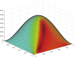
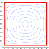
Figure 1: Stability region in the $2\times 2$ traffic game

When $a_{4}=0$ the characteristic polynomial can be factored as $p(\lambda)=\lambda q(\lambda)$ with $q(\lambda)={\lambda}^{3}+2{\lambda}^{2}+a_{2}\lambda+a_{3}$. So $p(\lambda)$ has a null eigenvalue. Applying the Routh-Hurwitz criterion to $q(\lambda)$ and using the inequalities $2a_{2}-a_{3}>0$ and $a_{3}>0$ in Lemma 3, it follows that the other three eigenvalues of $p(\lambda)$ have negative real part. Therefore, the equilibrium is still stable.

When $a_{4}$ becomes negative we have $p(0)=a_{4}<0$ and since $p(\pm\infty)=\infty$ it follows that there are at least one negative and one positive eigenvalue so that the rest point is an unstable saddle point for the dynamics. In fact, by a continuity argument, when $a_{4}$ is slightly negative, $a_{2}$ and $a_{3}$ are still positive and $p(\lambda)$ will have exactly one positive root and the other three roots have negative real part. Hence, for $a_{4}$ slightly positive, the rest point is unstable due to a crossing of the imaginary axis of a simple real negative root. This does not discard the presence of a Hopf bifurcation or other more complex dynamical behavior. The non-existence of Hopf bifurcation will be established later by a $K_{s}$-monotonicity argument.

Although we have established the existence of rest points, we have not yet determined how many of these equilibria exist. Using a fixed-point argument based on a one dimensional dynamical map associated with the dynamical system, we will see that depending on the values of the parameters there may be multiple equilibria.

4.2 Counting stable and unstable equilibria

We claim that in the $2\times 2$ case there are either one, two or three rest points. To see this we reduce (30) to a fixed point equation in dimension one. Namely, we note that a solution $x$ of (30) is fully determined once we know $\pi^{1a}$ and $\pi^{2a}$. Moreover, denoting $w^{i}=\beta_{i}(x^{ia}\!-\!x^{ib})$ these Logit probabilities are $\pi^{ia}=\rho(w^{i})$ where $\rho(w)=1/[1\!+\!\exp(w)]$ so that (30) can be reduced to a $2\times 2$ system in the unknowns $w^{1}$ and $w^{2}$. Indeed, substracting the equations in each block of (30) and setting $\varphi(w)=\kappa+\delta\rho(w)$ with $\kappa=C_{1}^{a}-C_{2}^{b}$, we get

$$\begin{array}[]{l}w^{1}=\beta_{1}\,\varphi(w^{2})\\ w^{2}=\beta_{2}\,\varphi(w^{1}).\end{array}$$ (43)

Hence $w^{1}$ is a fixed point of the scalar function $\psi(w)\triangleq\beta_{1}\varphi(\beta_{2}\varphi(w))$, which yields a solution of (43) with $w^{2}=\beta_{2}\,\varphi(w^{1})$. This establishes a one to one correspondence between the solutions of (30) and the fixed points of $\psi$. Moreover, using (45) and noting that $\varphi^{\prime}(w)\!=\!\delta\rho(w)(1\!-\!\rho(w))$ we get

$$\psi^{\prime}(w^{1}) = \nu\varphi^{\prime}(w^{2})\varphi^{\prime}(w^{1})$$ (44)

$$= \nu\delta^{2}\pi^{1a}(1\!-\!\pi^{1a})\pi^{2a}(1\!-\!\pi^{2a})$$

$$= \nu\delta^{2}\pi^{1a}\pi^{1b}\pi^{2a}\pi^{2b}$$

so that the rest point $x$ is stable if and only if $\psi^{\prime}(w^{1})<1$.

Theorem 2.

The function $\psi$ has either one, two or three fixed points, and exactly one of the following mutually exclusive situations occurs.

• $\psi$ has a unique fixed point $\bar{w}$ with $\psi^{\prime}(\bar{w})\leq 1$. The corresponding $\bar{x}$ is the unique equilibrium of (7) and it is stable iff $\psi^{\prime}(\bar{w})<1$.

• $\psi$ has two fixed points $w_{-}<w_{+}$ with either $\psi^{\prime}(w_{-})<1=\psi^{\prime}(w_{+})$ or $\psi^{\prime}(w_{+})<1=\psi^{\prime}(w_{-})$. The corresponding points $x_{-}$ and $x_{+}$ are the only rest points of (7). One of them is stable and the other is unstable.

• $\psi$ has three fixed points $w_{-}\!<\!\bar{w}\!<\!w_{+}$ with $\psi^{\prime}(w_{-})<1$, $\psi^{\prime}(w_{+})<1$, and $\psi^{\prime}(\bar{w})>1$. The corresponding points $x_{-}$, $x_{+}$ and $\bar{x}$ are the only rest points of (7), with $x_{+}$ and $x_{-}$ stable and $\bar{x}$ unstable.

Proof.

Let us first observe that when $\delta=0$ the function $\psi$ is constant and has a unique fixed point $\bar{w}=\beta_{1}\kappa$ which falls in the situation (a). Let us then consider the case $\delta>0$ so that $\varphi$ is strictly decreasing. In this case $\psi$ is strictly increasing and bounded so that it must cross the identity at least once. On the other hand, a direct calculation yields

$$\psi^{\prime}(w)\!\! = \nu\varphi^{\prime}(\beta_{2}\varphi(w))\varphi^{\prime}(w)$$ (45)

$$\psi^{\prime\prime}(w)\!\! = \nu\beta_{2}\varphi^{\prime\prime}({\beta}_{2}\varphi(w))\varphi^{\prime}(w)^{2}+\nu\varphi^{\prime}({\beta}_{2}\varphi(w))\varphi^{\prime\prime}(w)$$ (46)

$$= {}\!\!\frac{\nu\delta^{2}e^{\beta_{2}\varphi(w)}e^{2w}}{(1\!+\!e^{\beta_{2}\varphi(w)})^{2}(1\!+\!e^{w})^{4}}\left[\beta_{2}\delta-\frac{2\beta_{2}\delta}{1\!+\!e^{\beta_{2}\varphi(w)}}-2\sinh(w)\right]\!.$$

Recall that $\sinh x=\frac{1}{2}(e^{x}-e^{-x}),\;x\in\mathbb{R}$. The expression in the last square bracket is strictly decreasing in $w$ so that $\psi^{\prime\prime}$ has exactly one zero $w_{0}$ and therefore $\psi$ is strictly convex on $(-\infty,w_{0}]$ and strictly concave on $[w_{0},\infty)$. It follows that $\psi$ can cross the identity at most three times (see Fig. 2) and one of the mutually exclusive situations (a)-(c) must occur. ∎

Figure 2 below illustrates case (c) where $\psi$ has 3 fixed points with $\psi^{\prime}(\bar{w})>1$. Depending on the values of the parameters $\kappa,\delta$ and $\nu$, the graph of $\psi$ might shift to the right so that eventually $\bar{w}$ and $w_{+}$ may collapse into a single fixed point producing situation (b), after which this double fixed point disappears leading to case (a) with $w_{-}$ as the only fixed point. Symetrically, if the graph of $\psi$ is shifted to the left, $\bar{w}$ may collapse with $w_{-}$ producing situation (b), after which we fall into case (a) with unique fixed point $w_{+}$. Note that the case (a) with $\psi^{\prime}(\bar{w})=1$ can only occur when $\psi$ has an inflection at $\bar{w}$.

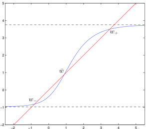
Figure 2: Three fixed points with $\psi^{\prime}(\bar{w})>1$.

Since $\psi$ is a strictly increasing function in one dimension, from dynamical system theory for maps [26], it follows that for generic cases in Theorem 2, the fixed point is an orientation preserving sink when ${\psi}^{{}^{\prime}}<1$ and an orientation reversing source if ${\psi}^{{}^{\prime}}>1$. In the latter case, two additional fixed points appear ($w_{-}$ and $w_{+}$) which correspond to two stable steady states of the ODE system, indicating a topological change in the structure of the mean field dynamics which exhibits a bifurcation of the fold kind [35].

In case of multiplicity the rest points satisfy an order relation. Namely, let $s=(1,-1,-1,1)$ and consider the partial order $\leq_{s}$ induced by the orthant

$$K_{s}=\{x\in{\mathbb{R}}^{4}:s_{i}x_{i}\geq 0\mbox{ for all }i=1,\ldots,4\},$$

that is to say, $x\leq_{s}y$ if and only if $s_{i}(y_{i}-x_{i})\geq 0$ for $i=1,\ldots,4$.

Proposition 1.

Consider case (c) in Theorem 2 where $\psi$ has three fixed points $w_{-}\!<\!\bar{w}\!<\!w_{+}$. Then the corresponding rest points $x_{-}$, $x_{+}$ and $\bar{x}$ are ordered as $x_{-}\leq_{s}\bar{x}\leq_{s}x_{+}$.

Proof.

Since $w^{1}_{-}=w_{-}<w_{+}=w^{1}_{+}$, and since $\rho(\cdot)$ is decreasing, the corresponding Logit probabilities satisfy the inequality

$$\pi^{1a}_{-}=\rho(w^{1}_{-})>\rho(w^{1}_{+})=\pi^{1a}_{+}$$

so that the third and fourth equations in (30) yield $x^{2a}_{-}\geq x^{2a}_{+}$ and $x^{2b}_{-}\leq x^{2b}_{+}$. Now, since $\varphi(\cdot)$ is decreasing it follows that $w^{2}_{-}=\beta_{2}\varphi(w^{1}_{-})>\beta_{2}\varphi(w^{1}_{+})=w^{2}_{+}$ and similarly as before we get

$$\pi^{2a}_{-}=\rho(w^{2}_{-})<\rho(w^{2}_{+})=\pi^{2a}_{+}$$

so that the first and second equations in (30) yield $x^{1a}_{-}\leq x^{1a}_{+}$ and $x^{1b}_{-}\geq x^{1b}_{+}$. Hence $x_{-}\leq_{s}x_{+}$. Analogous arguments yield $x_{-}\leq\bar{x}$ and $\bar{x}\leq_{s}x_{+}$. ∎

4.3 $K_{s}$-monotonicity and asymptotics of the dynamics

The symmetric sign distribution of the Jacobian coefficients in (36) motivates the use of results of monotone or order-preserving dynamical systems theory [45]. Such dynamical systems naturally occur in biology, chemistry, physics and economics, where the notion of cooperative vector field shows up. For those vector fields, a natural order relationship among trajectories rises which severely restricts the long-term behavior of the positive semi-flows. In the field of game theory, cooperative dynamics have been used to study the asymptotics of best response dynamics as well as fictitious play for supermodular games (see e.g. [6, 8, 9, 11, 31]). Here we use the results for $K_{s}$-monotonic dynamical systems to describe the global behavior of the learning dynamics in the $2\times 2$ traffic game. Note however that, in contrast with the previously cited applications in games, the nature of congestion games leads to competitive rather than cooperative dynamics.

Let $s=(1,-1,-1,1)$ as in the previous section. The dynamics (7) turn out to be $K_{s}$-monotone, which gives a more complete picture of its asymptotic behavior. Recall [45, Smith] that a flow ${\phi}_{t}(x_{0})$ generated by a system of ordinary differential equations

$$\left\{\begin{array}[]{l}\dot{x}(t)=f(x(t)),\\ x(0)=x_{0}\end{array}\right.$$

is called $K_{s}$-monotone if it preserves the partial order $\leq_{s}$, namely, for all $x_{0},y_{0}\in U$ such that $x_{0}\;{\leq}_{s}\;y_{0}$ it holds that ${\phi}_{t}(x_{0})\;{\leq}_{s}\;{\phi}_{t}(y_{0})$ for all times $t\geq 0$ at which both solutions are defined.

We will use Lemma 2.1 in [45, Smith] which gives necessary and sufficient conditions for the flux of an ODE system to be $K_{s}$-monotone in terms of the signs of the entries of the Jacobian matrix of the system.

Proposition 2.

Consider a $2\times 2$ traffic game. Then,

• The mean field system (7) is $K_{s}$-monotone for $s=(1,-1,-1,1)$.

• If there exists some $T>0$ such that $\phi_{T}(x_{0})\!<_{s}\!x_{0}$ or $x_{0}\!<_{s}\!\phi_{T}(x_{0})$, then the orbit $\phi_{t}(x_{0})$ converges to a rest point as $t\to\infty$.

Proof.

According to [45, Lemma 2.1], a system is $K_{s}$-monotone if and only if for all $x\in U$ the matrix $P_{s}J(x)P_{s}$ has non-negative off-diagonal elements, where $J(x)=Df(x)$ and $P_{s}=\mbox{diag }(s_{1},\ldots,s_{n})$. Since the Jacobian of (7) is given by (36), the off-diagonal terms $(P_{s}J(x)P_{s})_{ij}=s_{i}s_{j}J_{ij}$ are non-negative if and only if

$$s_{1}s_{3}<0~{};~{}s_{1}s_{4}>0~{};~{}s_{2}s_{3}>0~{};~{}s_{2}s_{4}<0.$$

This holds for $s=(1,-1,-1,1)$ proving assertion a).

In order to prove b) we first note that for all $i,r$ we have $C^{ir}\!(x^{\mbox{-}i})\in[C_{1}^{r},C_{N}^{r}]$, from which it follows that all the forward orbits of (7) are bounded. Moreover, since the Jacobian (36) has only one zero in each row and column, then $J(x)$ is irreducible in the sense of [45]. Hence we may invoke [45, Lemma 2.3(b)] which asserts precisely that the existence of $T>0$ with either $\phi_{T}(x_{0})<_{s}x_{0}$ or $\phi_{T}(x_{0})>_{s}x_{0}$ implies that the orbit $\phi_{t}(x_{0})$ converges to a rest point. ∎

Theorem 3.

Consider the mean field dynamics (7) for a $2\times 2$ traffic game. Then for almost all initial conditions $x_{0}\in\mathbb{R}^{4}$ the corresponding orbit $x(t)=\phi_{t}(x_{0})$ converges to a rest point. Moreover, the union of the basins of attraction of all the steady states is dense in $\mathbb{R}^{4}$.

Proof.

We already noted that all forward orbits of (7) are bounded, and also that there are finitely many rest points. Also, from Proposition 2 we know that (7) is $K_{s}$-monotone and irreducible. Hence [45, Theorem 2.5] asserts precisely that the orbits $\phi_{t}(x_{0})$ converge towards a rest point for almost all initial conditions $x_{0}\in\mathbb{R}^{4}$, which establishes the first claim.

In order to prove the second assertion we use [45, Theorem 2.6] which states that if $X_{0}$ is an open, bounded, positively invariant set for a $K_{s}$-monotone system, whose closure $\bar{X}_{0}$ contains finitely many rest points $E$, then the union of the interiors of the basins of attraction $B_{e}$ of these rest points $\cup_{e\in E\cap\bar{X}_{0}}\mathop{\rm int}(B_{e})$ is dense in $X_{0}$. In our setting we may apply this result to an open rectangle $X_{0}=(-R,R)^{4}$ with $R>\max\{C^{a}_{2},C^{b}_{2}\}$, which is easily seen to be positively invariant for the mean field dynamics (7). Then the union of the basins of attraction of the (finitely many) rest points is dense in $(-R,R)^{4}$ and we conclude by letting $R\to\infty$. ∎

According to [45, Lemma 2.2] the matrix $P_{s}(\frac{\partial{\phi}_{t}}{\partial x_{0}}(x_{0}))P_{s}$ has all its entries strictly positive for all $t>0$, and therefore (7) cannot have an attracting closed orbit nor two points of an $\omega$-limit set related by ${\leq}_{s}$. Also, by the Perron-Frobenius Theorem [39] the spectral radius of $P_{s}(\frac{\partial{\phi}_{t}}{\partial x_{0}}(x_{0}))P_{s}$ is a positive simple eigenvalue strictly larger in modulus than all the remaining eigenvalues, and the corresponding eigenvector is positive. For further properties of totally positive matrices we refer to [1].

Let us also observe that the Jacobian $J(x)$ has an eigenvalue equal to

$$s(J(x))=\max\{\Re({\lambda}):\lambda\mbox{ eigenvalue of }J(x)\}.$$

Theorem 2.7 in [45] provides a set of equivalent conditions for the stability condition $s(J(x))<0$. In particular, condition (iv) in [45, Theorem 2.7] matches Routh-Hurwitz criterion [41], while the Gerschgorin criterion [40] follows from condition (ii) in [45, Theorem 2.7].

From a bifurcation analysis viewpoint, a rest point loses stability when a simple real eigenvalue crosses from negative to positive [26]. Therefore, locally stable Hopf bifurcations cannot occur for $K_{s}$-monotone systems, although unstable Hopf bifurcations cannot be excluded [35]. The only local bifurcation involving an exchange of stability that a steady state can be involved in is a steady state bifurcation. The next result provides additional information on the dynamics (7) in the presence of an unstable equilibrium. Recall that in this case there are 3 rest points $x_{-}\leq_{s}\bar{x}\leq_{s}x_{+}$ with $\bar{x}$ unstable and the other two stable.

Theorem 4.

Consider the case (c) in Theorem 2 where $\psi$ has three fixed points $w_{-}\!<\!\bar{w}\!<\!w_{+}$. Then the unstable equilibrium $\bar{x}$ is connected by two monotone heteroclinic orbits to the stable rest points $x_{-}$ and $x_{+}$.

Proof.

The matrix $J(\bar{x})$ is similar to $A=P_{s}J(\bar{x})P_{s}$ which is irreducible and has non-negative off-diagonal entries. Hence for $\alpha>0$ large enough $\alpha I+A$ is non-negative and irreducible so that by the Perron-Frobenius Theorem we have that $s(\alpha I+A)=\alpha+s(J(\bar{x}))$ is a simple eigenvalue of $\alpha I+A$ with corresponding eigenvector $v\geq 0$. It follows that $\bar{s}=s(J(\bar{x}))$ is a simple eigenvalue of $J(\bar{x})$ with eigenvector $\bar{v}=P_{s}v$, and since $\bar{x}$ is unstable we have $\bar{s}>0$. The conclusion then follows by a straightforward application of [45, Theorem 2.8] which establishes the existence of two $C^{1}$ heteroclinic curves $y_{+}:[0,\infty)\to\mathbb{R}^{4}$ and $y_{-}:[0,\infty)\to\mathbb{R}^{4}$ such that

• $y_{\pm}(r)=\bar{x}\pm r\bar{v}+o(r)$ for $r\to 0$ and $y_{\pm}(r)\to x_{\pm}$ for $r\to\infty$,

• for each $r\geq 0$ the orbits started from $y_{\pm}(r)$ follow these curves and are given by $\phi_{t}(y_{\pm}(r))=y_{\pm}(re^{\bar{s}t})$ for all $t\geq 0$, and

• for all $0\leq r_{1}\leq r_{2}$ we have $y_{+}(r_{1})\leq_{s}y_{+}(r_{2})$ and $y_{-}(r_{2})\leq_{s}y_{-}(r_{1})$.

∎

Even though a $K$-monotone system cannot have an attracting periodic orbit, when time is reversed these systems often do have attracting closed orbits. It can be shown that every closed orbit has a simple Floquet multiplier [35] which exceeds unity. This largest multiplier gives rise to a very unstable cylinder manifold associated with the closed orbit which has monotonicity properties [45]. In the specific case of (7) we do not know whether the time reversed dynamics have an attracting closed orbit or not.

4.4 The $2\times 2$ case with symmetric players

Theorem 2 establishes three possible situations for the number and stability of the rest points of the mean field dynamics. However, it does not provide explicit conditions on the data of the traffic game to predict which situation will occur. We will show next that this is possible when the two players are identical with $\beta_{1}=\beta_{2}$. In the sequel we denote $\beta$ this common value. Introducing the function $\theta(w)=\beta\varphi(w)$, the system (43) becomes

$$\begin{array}[]{l}w^{1}=\theta(w^{2})\\ w^{2}=\theta(w^{1})\end{array}$$ (47)

so that both $w^{1}$ and $w^{2}$ are fixed points of $\psi(w)=\theta\circ\theta(w)$.

Now, the function $\theta(w)$ decreases from $\beta(\kappa+\delta)$ at $w=-\infty$ to $\beta\kappa$ at $w=\infty$, so that it has a unique fixed point $\bar{w}=\theta(\bar{w})$. This yields a unique symmetric solution $w^{1}=w^{2}=\bar{w}$ for (47), which corresponds to a symmetric rest point $\bar{x}$ with $\bar{x}^{1a}=\bar{x}^{2a}$ and $\bar{x}^{1b}=\bar{x}^{2b}$.

Note that if $\psi$ admits another fixed point $w^{1}\neq\bar{w}$ then $w^{2}=\theta(w^{1})$ is also a fixed point. Since $\theta$ is decreasing, if $w^{1}<\bar{w}$ then $w^{2}>\bar{w}$ and viceversa so that $\bar{w}$ is always the centermost fixed point of $\psi$. Hence case (b) in Theorem 2 cannot occur and $\psi$ has either one or three distinct fixed points.

Theorem 5.

Consider a $2\times 2$ symmetric traffic game. Let $\bar{x}$ be the symmetric rest point associated with the unique fixed point $\bar{w}$ of $\theta$.

• If $\psi^{\prime}(\bar{w})\leq 1$ then $\bar{w}$ is the only fixed point of $\psi$ and $\bar{x}$ is the unique rest point of (7). This rest point is stable if and only if $\psi^{\prime}(\bar{w})<1$.

• If $\psi^{\prime}(\bar{w})>1$ then $\psi$ has exactly three fixed points $w^{1}<\bar{w}<w^{2}$ with $w^{1}\!=\!g(w^{2})$ and $w^{2}\!=\!g(w^{1})$, and we have

  $$\psi^{\prime}(w^{1})=\psi^{\prime}(w^{2})=\theta^{\prime}(w^{1})\theta^{\prime}(w^{2})\!<\!1.$$

  The symmetric rest point $\bar{x}$ is unstable and there are two stable non-symmetric equilibria: one defined by $\pi^{1a}=\rho(w^{1}),\pi^{2a}=\rho(w^{2})$, and the other one with the identities of the players exchanged.

Proof.

This follows from the previous comments and Theorem 2. ∎

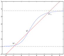
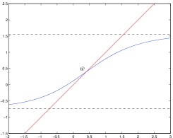
Figure 3: Fixed points of $\psi$: $\psi^{\prime}(\bar{w})>1$ (left) vs $\psi^{\prime}(\bar{w})<1$ (right).

As seen above, in the symmetric case the number of rest points and their nature are completely determined by the condition $\psi^{\prime}(\bar{w})<1$. The latter can be checked directly from the data definining the game. More precisely, denoting

$$c=(C_{1}^{a}+C_{2}^{a})-(C_{1}^{b}+C_{2}^{b})$$ (48)

we have the following characterization established in [38]. For the sake of completeness we include a proof. We recall that the hyperbolic arctangent function is defined by $\mathop{\rm arctanh}x=\frac{1}{2}\ln\left(\frac{1+x}{1-x}\right)$ for $x\in(-1,1)$.

Proposition 3.

Consider the parameters $\mu=\beta\delta$ and $q=c/\delta$, as well as the function $h(x)=x\,\mathop{\rm arctanh}\sqrt{1\!-\!x}\,+\sqrt{1\!-\!x}$. Then $\psi^{\prime}(\bar{w})<1$ if and only if $|q|<h(4/\mu)$.

Proof.

Noting that $\psi^{\prime}(\bar{w})=\theta^{\prime}(\bar{w})^{2}$ the condition $\psi^{\prime}(\bar{w})<1$ is equivalent to $\theta^{\prime}(\bar{w})<-1$. Since $\theta^{\prime}(\bar{w})=-\beta\delta e^{\bar{w}}(1+e^{\bar{w}})^{-2}$, denoting $\bar{z}=1+e^{\bar{w}}$ this can be written as $\mu(\bar{z}-1)>\bar{z}^{2}$ which translates into the fact that $\bar{z}$ lies strictly between the roots of $z^{2}-\mu\bar{z}+\mu=0$, that is $z_{-}<\bar{z}<z_{+}$ where

$$z_{\pm}=\mbox{$\frac{1}{2}$}[\mu\pm\sqrt{\mu(\mu-4)}].$$ (49)

Denoting $w_{\pm}=\ln(z_{\pm}-1)$ this is equivalent to $w_{-}<\bar{w}<w_{+}$. Since $\bar{w}$ is the fixed point of $\theta(\cdot)$ and since this function is decreasing, this is in turn equivalent to the two inequalities

$$\theta(w_{-})>w_{-}\quad;\quad\theta(w_{+})<w_{+}.$$

Now, observing that $\theta(w_{\pm})=\beta\kappa+\beta\delta/z_{\pm}$, the latter can be written as

$$\ln(z_{-}-1)-\frac{\beta\delta}{z_{-}}<\beta\kappa<\ln(z_{+}-1)-\frac{\beta\delta}{z_{+}}.$$

Replacing the expression (49) for $z_{\pm}$ and denoting

$$f_{\pm}(\mu)=\frac{1}{\mu}\ln\left(\frac{\mu\pm\sqrt{\mu(\mu-4)}}{2}-1\right)-\frac{2}{\mu\pm\sqrt{\mu(\mu-4)}}$$

these inequalities can be expressed as

$$f_{-}(\mu)<\frac{\kappa}{\delta}<f_{+}(\mu).$$ (50)

Now, by direct computation one can check that $f_{-}(\mu)+f_{+}(\mu)=-1$ so that, setting $g(\mu)=2f_{+}(\mu)+1$, we may restate (50) in the symmetric form

$$-g(\mu)<1+\frac{2\kappa}{\delta}<g(\mu).$$

The conclusion follows by noting that $1+2\kappa/\delta=q$ and $g(\mu)=h(4/\mu)$. ∎

Figure 4 illustrates the stability region for the $2\times 2$ symmetric game. This plot confirms that for $\mu=\beta\delta<4$, which is equivalent to the condition $\nu\delta^{2}<16$ in the comment after Theorem 1, the symmetric equilibrium $\bar{x}$ is the unique rest point and it is stable. When $\theta^{\prime}(\bar{w})$ crosses the value $-1$ the symmetric steady state loses stability and two new stable equilibria appear. This is due to the crossing of the imaginary axis by a simple negative eigenvalue. Bifurcation theory for maps also predicts this situation which is indicative of a fold bifurcation (see [35]).

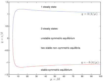
Figure 4: Stability region for a $2\times 2$ symmetric game in the $\mu$-$q$ parameters.

5 Summary and future work

In this paper, we gave a necessary and sufficient condition for the stability of equilibria for a $2\times 2$ symmetric traffic game. The main tool used was the Routh-Hurwitz stability criterion for dynamical systems. We also exploited the results for $K$-monotone systems to establish the asymptotic convergence of the mean field dynamics.

With respect to Proposition 3 we conjecture that the condition $|q|<h(4/\beta\delta)$ for having a unique stable equilibrium might still hold for the case of non-symmetric players provided that we take $\beta=\sqrt{\beta_{1}\beta_{2}}$.

The extension to the general case with $M$ routes and $N$ players seems much more difficult. However our numerical simulations show that the dynamics still converge to equilibria and exhibit a certain regularity in the structure of the attractors. Namely, for the case with identical players $\beta_{i}\equiv\beta$, there is a unique symmetric equilibrium in which $\bar{x}^{ir}=\bar{x}^{jr}$ for all routes $r$ and different players $i,j$. When $\beta$ is small this is the only rest point and a global attractor, whereas for larger $\beta$ the symmetric equilibrium becomes unstable and there appear non-symmetric rest points $(x^{i})_{i\in I}$ with $x^{i}\neq x^{j}$ for some $i\neq j$. However, these non-symmetric equilibria exhibit clusters of players with the same estimate vector $x^{i}$’s and, interestingly, the number of players in each cluster is stable across the different equilibria. It would be interesting to understand the reasons for such stable structure.

Another possible line of research is to investigate the extension of the results from routing games to general 2-player games and beyond. Although some asymptotic results were already described in [14] for the adaptive dynamics in general finite games, they hold only in the regime where the Logit parameters $\beta_{i}$ are small. Since the results in this paper strongly exploit the symetric structure of the Jacobian matrix in §3, it is unclear if and how the arguments could be adapted to general games.

References

- [1] Ando T., Totally Positive Matrices, Linear Algebra and Its Applications, Volume 90, pp. 165-219, May 1987. doi:10.1016/0024-3795(87)90313-2.
- [2] Arthur W.B., On designing economic agents that behave like human agents, J. Evolutionary Econ. 3, 1–22, (1993).
- [3] Auer P., Cesa-Bianchi N., Freund Y. and Schapire R.E., The non-stochastic multiarmed bandit problem, SIAM J. on Computing 32, 48–77, (2002).
- [4] Avinieri E., Prashker J., The impact of travel time information on travellers’ learning under uncertainty, paper presented at the 10th International Conference on Travel Behaviour Research, Lucerne, (2003).
- [5] Beggs A., On the convergence of reinforcement learning, Journal of Economic Theory 122, 1–36, (2005).
- [6] A. Beggs, Learning in Bayesian games with binary actions, B. E. J. Theor. Econ. 9, 30, (2009).
- [7] Benaïm M., Dynamics of stochastic approximation algorithms, in Séminaire de Probabilités, Lecture Notes in Math. 1709, Springer, Berlin, 1–68, (1999).
- [8] Benaïm M. and Faure M., Stochastic approximation, cooperative dynamics and supermodular games, Ann. Appl. Probab. 22(5), pp. 2133-2164, (2012).
- [9] Benaïm M. and Hirsch M.W., Stochastic approximation algorithms with constant step size whose average is cooperative. Ann. Appl. Probab. 9, pp. 216 241, (1999).
- [10] Börgers T., Sarin R., Learning through reinforcement and replicator dynamics, Journal of Economic Theory 77, 1–14, (1997).
- [11] Borkar V., Cooperative dynamics and Wardrop equilibria, Systems & Control Letters 58(2), pp. 91-93, (2009).
- [12] Bravo M., An adjusted payoff-based procedure for normal form games, Mathematics of Operations Research, Volume 41, Issue 4, pp 1469-1483, September 2016.
- [13] Brown G., Iterative solution of games by fictitious play, in Activity Analysis of Production and Allocation, Cowles Commission Monograph No. 13. John Wiley & Sons, Inc., New York, N.Y., 374–376, (1951).
- [14] Cominetti R., Melo E., Sorin S., A payoff based learning procedure and its application to traffic games, Games and Economic Behavior, 70 (2010) 71-83.
- [15] Coste M., An introduction to O-minimal geometry, Institut de Recherche Mathématique de Rennes, November 1999.
- [16] R. Cressman, The Stability Concept of Evolutionary Game Theory: A Dynamic Approach, Springer-Verlag Berlin Heidelberg, 1992.
- [17] Daganzo C., Sheffi Y., On stochastic models of traffic assignment, Transportation Science 11, 253–274, (1977).
- [18] Dimitrov D.K., Peña J.M., Almost strict total positivity and a class of Hurwitz polynomials, Journal of Approximation Theory, 132 (2005) 212-223.
- [19] Erev I. and Roth A.E., Predicting how people play games: Reinforcement learning in experimental games withunique, mixed strategy equilibria, American Economic Review 88, 848–881, (1998).
- [20] Fisk C., Some developments in equilibrium traffic assignment, Transportation Research 14B, 243–255, (1980).
- [21] Foster D., Vohra R.V., Calibrated learning and correlated equilibria, Games and Economic Behavior 21, 40-55, (1997).
- [22] Foster D., Vohra R.V., Asymptotic calibration, Biometrika 85, 379-390, (1998).
- [23] Freund Y. and R.E. Schapire, Adaptive game playing using multiplicative weights, Games and Economic Behavior 29, 79-103, (1999).
- [24] Fudenberg D., Levine D.K., The Theory of Learning in Games, MIT Press, Cambridge, MA, (1998).
- [25] Gantmacher F.R., Applications of the Theory of Matrices, Interscience, New York, 641 (9), 1-8, 1959.
- [26] Guckenheimer J., Holmes P., Nonlinear Oscillations, Dynamical Systems, and Bifurcations of Vector Fields, Springer-Verlag, New York, 5th edition, 1997.
- [27] Hannan J., Approximation to Bayes risk in repeated plays, in Contributions to the Theory of Games (Vol. 3), edited by M. Dresher, A. W. Tucker, and P. Wolfe, Princeton Univ. Press, 97–139, (1957).
- [28] Hart S., Adaptive heuristics, Econometrica 73, 1401–1430, (2002).
- [29] Hart S., Mas-Colell A., “A reinforcement procedure leading to correlated equilibrium”, in Economics Essays: A Festschrift for Werner Hildenbrand, edited by G.
- [30] Hofbauer J., Sandholm W.H., On the global convergence of stochastic fictitious, Econometrica 70, 2265–2294, (2002).
- [31] Hofbauer J. and. Sandholm W, On the global convergence of stochastic fictitious play, Econometrica 70, pp. 2265 2294, (2002).
- [32] J. Hofbauer and K. Sigmund, Evolutionary Games and Population Dynamics, Cambridge University Press, United Kingdom, 1998.
- [33] Horowitz J., The stability of stochastic equilibrium in a two-link transportation network, Transportation Research Part B 18, 13–28, (1984).
- [34] Kushner H.J., Yin G.G., Stochastic Approximations Algorithms and Applications, Applications of Mathematics 35, Springer-Verlag, New York, (1997).
- [35] Kuznetsov Y.A., Elements of Applied Bifurcation Theory, Springer-Verlag, New York, 2nd edition, 1995.
- [36] Laslier J.-F., Topol R. and Walliser B., A behavioral learning process in games, Games and Economic Behavior 37, 340–366, (2001).
- [37] McKelvey R., Palfrey T., Quantal response equilibria for normal form games, Games and Economic Behavior 10, 6–38, (1995).
- [38] Maldonado F.A., Estudio de una dinámica adaptativa para juegos repetidos y su aplicación a un juego de congestión, Memoria, Universidad de Chile, Facultad de Ciencias Físicas y Matemáticas, Departamento de Ingeniería Matemática, Santiago, Chile, 2012.
- [39] Meyer C.D., Matrix Analysis and Applied Linear Algebra, SIAM, Philadelphia, 2000.
- [40] Morton K.W. and Mayers D., Numerical Solution of Partial Differential Equations, Cambridge University Press, 2nd Edition, 2005.
- [41] Murray J. D. , Mathematical Biology, 2nd Edition, Springer, Berlin, Germany, 1993.
- [42] Posch M., Cycling in a stochastic learning algorithm for normal form games, J. Evol. Econ. 7, 193–207, (1997).
- [43] Robinson J., An iterative method of solving a game, Ann. Math. 54, 296–301, (1951).
- [44] Rosenthal R.W., A class of games possessing pure-strategy Nash equilibria, International Journal of Game Theory 2, 65–67, (1973).
- [45] Smith H.L., Systems of Ordinary Differential Equations Which Generate an Order Preserving Flow. A Survey of Results, SIAM Review, Vol. 30, No. 1, pp. 87-113, March 1988.
- [46] Selten R., Chmura T., Pitz T., Kube S., Schreckenberg M., Commuters route choice behaviour, Games and Economic Behavior 58, 394–406, (2007).
- [47] van den Dries L., -Minimal Structures and Real Analytic Geometry, Current Development in Mathematics, 1988.
- [48] Wardrop J., Some theoretical aspects of road traffic research, Proceedings of the Institution of Civil Engineers Vol. 1, 325–378, (1952).
- [49] Young P., Strategic Learning and its Limits, Oxford University Press, (2004).