Non uniform weighted extended B-Spline finite element analysis of non linear elliptic partial differential equations.

Abstract

We propose a non uniform web spline based finite element analysis for elliptic partial differential equation with the gradient type nonlinearity in their principal coefficients like p-laplacian equation and Quasi-Newtonian fluid flow equations. We discuss the well-posednes of the problems and also derive the apriori error estimates for the proposed finite element analysis and obtain convergence rate of $\mathcal{O}(h^{\alpha})$ for $\alpha>0$.

1 Introduction

Finite element method is one of the popular numeraical techniques for solving partial differential equation’s modeling real life problems from science and engineering. Currently there is marked interest for meshless approach for solving boundary value problems as it significantly saves the cost and trouble of generating mesh, which infinitesimal in many cases may turn out to be the computationally the most expensive job.Weighted extended B-splines is a finite element method (fem) in a infinitesimal cost mesh framework. The present work on nonlinear elliptic problems is based on non-uniform weighted extended b-splines (NUWEBS)fem this which was originally proposed by H$\ddot{o}$llig et al hollig2001weighted; hollig2003nonuniform; hollig2003finiteon trivial mesh framework. The p-laplacian equation used into the design of shock free airfoil and non-Newtonian fluid flow model used in understanding seepage through coarse grained porous media in some geological problems etc have gradient type non linearity in their principal coefficients. They also occur in the description of non linear diffusion and filtration repin2000posteriori , power law materials murthy2015parallel and Quasi Newtonian flows barrett1994quasi.Earlier in a grid based framework mixed finite element methods were developed and analyzed in melenk1996partition; arbogast1992existence for elliptic problems. Here we are concerned with the finite element analysis in a gridless framework and provide the convergence analysis of weighted extended b-spline finite element analysis for p-laplacian equation and Quasi-Newtonian flow model.
An outline of the paper is as follows. We present some preliminary knowledge on the non-uniform weighted extended b-spline (WEB-S) space in section (2) and establish an optimal order a priori error estimates of p-Laplacian problem in section (4).We discuss Quasi -Newtonian problems in ( 5).Furthermore,throughout our discussion $\Omega$ is a bounded, multiply connected domian , i.e, it may contain holes and we use the symbols $\preceq,\succeq~{}\text{or}~{}\asymp$ instead $\leq,\geq~{}\text{or}~{}=$ whenever the constants are clear from the context and independent of the parameters.

2 Non uniform weighted extended B-Splines

Let $\Omega_{h}$ be a webs fem approximation to $\Omega$ defined by $\Omega_{h}=\cup_{i}\Omega_{h_{i}}$ where $\Omega_{h_{i}}$ is a partitioning of $\Omega_{h}$ into a finite number of disjoint open regular domains , each of maximum diameter bounded above by h . In addition, for any two distinct domains, their closures are either disjoint, or have a common boundaries. Associated with $\Omega_{h}$ is the finite-dimensional space $\mathcal{B}_{h}$ ( see below)

We can approximate a function on a bounded domain $\Omega\subset\mathbb{R}^{n}$ by forming a spline, i.e., a linear combination of all relevant B-splines

$$b_{k}~{}~{},k\in\mathbb{K}$$

which have some support in $\Omega$. Depending on the degree, this yields approximations of arbitrary order and smoothness. However, numerical instabilities may arise due to the outer B-splines

$$b_{j}~{}~{},j\in\mathbb{J}$$

for which no complete grid cell of their support lies in $\Omega$. Here and in the sequel, a grid cell is an interval which in every coordinate direction is bounded by two consecutive, but different knots, and an inner grid cell is a grid cell whose interior is completely contained in $\Omega$. A further difficulty is that, in general, splines do not conform to homogeneous boundary conditions, which is essential for standard finite element schemes zienkiewicz2000finite or for matching boundaries in data fitting problems. Fortunately, both problems can be resolved. A stable basis is obtained by forming appropriate extensions of the inner B-splines

$$b_{i}~{}~{},i\in\mathbb{I}=\mathbb{K}\sim\mathbb{J}$$

which have at least one inner grid cell in their support. Readers are refer to hollig2003finite; chaudhary2015web; de2013box for details description.

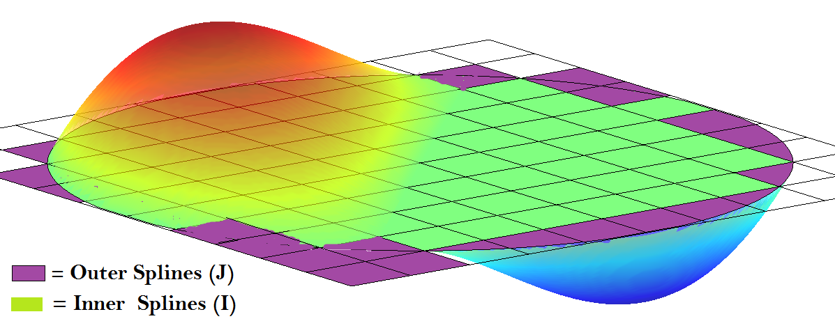
Figure 1: WEB-Splines

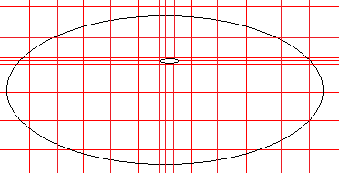
Figure 2: Non-uniform WEBS

2.1 Splines on Bounded Domains

The Splines $\mathbb{B}^{n}_{h}(D)$ on a bounded domain D$\subset$ $\mathbb{R}^{m}$ consist of all linear combinations $\sum\limits_{k\epsilon\mathbf{K}}c_{k}b^{n}_{k,h}$ of relevant B-Splines; i.e, the set $\mathbf{K}$ of relevant indices contains all k with $b^{n}_{k,h}(x)\neq$0 for some x $\epsilon$ D,where $b^{n}_{k,h}(x)=b^{n}(x/h-k)$ is the scaled translates.

2.2 Inner and Outer Splines

Grid cells $\mathbb{Q}$ = h ($[0,1]^{m}$ + $l$) are partitioned into interior, exterior and boundary cells depending on whether $\mathbb{Q}\subseteq\bar{D}$ , the interior of $\mathbb{Q}$ intersects $\partial D$ , or $\mathbb{Q}\cap D=\phi$. Among the relevant B-Splines,$b_{k},k$$\varepsilon$ K, distinction made between inner B-Splines

$b_{i}$,i $\varepsilon$ I

which have at least one interior cell in their support, and outer B-Splines

$b_{j}$,j $\varepsilon$ J=K$\backslash$I

for which supp $b_{j}$ consists entirely of boundary and exterior cells.

Theorem 2.1

The Spline

$p=\sum_{k\varepsilon K}q(k)b_{k}$

is a polynomial of order n on D iff $q$ is a polynomial of order n on K.

We assume that the boundary are smooth so that smooth solution could exist. As usual, the solution is approximated by a linear combination

$\sum_{i}a_{i}B_{i}$

of basis functions $B_{i}$ which vanish outside a set with diameter $\asymp$ h.Moreover, the basis functions are required to vanish on the boundary so we simply multiply by a fixed weight function w which satisfy the criteria, and in addition w is to be smooth and $\asymp$ dist(x,D).Readers are suggested de1988cardinal,rvachev1995r for more details

Definition 2.1 ( Extended b (eb) splines )

For $i\in I(j),j\in J(i)~{}and~{}Q_{j}$ we denote by $p_{i,j}$ the polynomial which agrees with $b_{i}~{}on~{}Q_{j}$ and define the extension coefficients

$$e_{i,j}=\lambda_{j}p_{i,j}$$

Then, the extended B-splines (eb-splines) are

$$B_{i}=b_{i}+\sum\limits_{j\in J(i)}e_{i,j}b_{j}~{}~{}i\in I(j)$$

where,the set of related inner indices is defined by $I(j)$ for an outer index, and $Q_{j}$ is an inner grid cell which is closest to supp $b_{j}~{}for~{}j\in J$ with respect to the Hausdorff metric , conversely for an inner index we define the set of related outer indices by $J(i)$.

Theorem 2.2

eb-splines and de Boor Fix functionals $\{\lambda_{k}\}$ are bi-orthogonal,i.e.

$$\lambda_{k}B_{k^{\prime}}=\delta_{k,k^{\prime}}~{}~{}~{}k,k^{\prime}\in\mathbb{Z}$$

In addition if $Q$ is an inner grid cell in the support of $B_{k}$ with length bounded by $|Q|\geq\alpha|suppB_{k}|$ for some constant $\alpha\in(0,1]$,then

$$|\lambda_{k}p|\leq const(n,\alpha)||p||_{\infty,Q}~{}~{}p\in\mathcal{P}_{n}$$

where,$|\cdot|~{}\textrm{represents measure of a set and}~{}\mathcal{P}_{n}$ is a linear space of polynomials of degree $\leq$ n

Generalizing the univariate definitions and results of the to $n\geq 2$ variables is straightforward. The arguments are completely analogous. Merely the notation needs to be adapted to the multivariate setting.We consider a tensor product grid in $\mathbb{R}^{n}$ with knot sequences $t=[t^{1},\ldots,t^{n}]$

$$t^{\nu}:\ldots\leq t^{\nu}_{k}\leq t^{\nu}_{k+1}\leq\ldots,~{}~{}\nu=1,\ldots,n$$

and denote by,

$$b_{k}=b^{m_{1}}_{k^{1},t_{1}}(x_{1})\ldots b^{m_{n}}_{k^{n},t_{n}}(x_{n})~{},~{}k\in\mathbb{Z}^{n}$$

the corresponding tensor product B-splines of degree $m=[m_{1},\ldots,m_{n}]$

Definition 2.2

Let $w$ be a positive weight function which is smooth on $\Omega$ and equivalent to some power $r\geq 0$ of the boundary distance function

$$w(x)\asymp dist(x,\partial\Omega)^{r}$$

and denote by $x_{i}$ the center of an inner grid cell in supp $b_{i}$.Then, the weighted extended B-splines (web splines) are defined by

$$B_{i}=\frac{w}{w(x_{i})}\biggl{(}b_{i}+\sum\limits_{j\in J(i)}e_{i,j}b_{j}\biggr{)}~{}~{}i\in I(j)$$

Theorem 2.3 (Jackson’s Inequality)

Let $u\in W^{1,p}(\Omega)$ . Then

$$||u-\mathcal{P}_{h}u||_{1}\leq\mathcal{O}(h).$$

2.3 Remark

• Theorem 2.2 remain valid for this new class of Splines.

• The linear span of web-splines is the web-space $\mathcal{B}$

• The canonical projector $\mathrm{P}_{h}$ onto the spline space $\mathcal{B}$ is defined as

  $$\mathrm{P}_{h}f=\sum\limits_{i\in\mathbb{I}}(\Lambda_{i}f)B_{i}$$ (1)

  where,the weight functional $\Lambda_{i}f=w(x_{i})\lambda_{i}(f/w)~{},~{}~{}i\in\mathbb{I}$, with $x_{i}$ as in definition 2.2

• It satisfies,

  $$\int_{\Omega}\nabla\cdot\left(\mathrm{P}_{h}u-u_{h}\right)v_{h}\,dx=0$$ (2)

3 Elliptic partial differential equation analysis in NUWEBSFEA framework

As NUWEBSFEA of variable coefficient of Poisson equation (VCPEA) is not available in literature, for simplicity we begin with NUWEBSFEA of VCPEA

The computational domain is denoted by $\Omega$ and and the VCPE model is given by,

$$-\nabla.a(x)\nabla u(x) =f(x)~{}~{}\text{on}~{}\Omega$$ (3)

$$u=0~{}~{}\text{on}~{}\partial\Omega$$ (4)

where $u$ is the scalar potential and $f$ is the source term. In case of EEG imaging this equation can often be used under the quasi static approximation of the Maxwell’s equation. Moreover in EEG the source term is like the form $f(x)=\nabla\cdot d(x)$ where , $d:\Omega\rightarrow\mathbb{R}^{m}~{}~{},~{}m=2,3$ is a vector field that describes the neural sources as idealized electric dipoles.
As usual the solution is approximated by a linear combination

$$u_{h}=\sum_{i}a_{i}B_{i}$$

which vanish outside a set of diameter proportional to grid width $h$.The coefficients $a_{i}$ ’s are determined from Galerkin system

$$\int a(x)\nabla B_{j}\nabla u_{h}\,dx=\sum_{i}\left(\int a(x)\nabla B_{j}\nabla B_{i}\,dx\right)a_{i}=\int B_{j}f$$ (5)

Theorem 3.1

Let, $u\in H^{n}$ be the solution of the problem (3) and $u_{h}=\sum_{i}a_{i}B_{i}$ a finite element approximation obtained by solving the Galerkin system (5) If there exist a $\kappa>0$ such that $a(x)\geq\kappa$ then

$$||u-u_{h}||_{1}\preceq h^{n-1}||u||_{1}$$

Proof

The proof relies on results and techniques from hollig2003nonuniform; de2013box and the theory of weighted approximations.Moreover, the standard error estimates for splines are crucial for our arguments. We begin by noting that,

$$||u||\preceq||a(x)u||~{}~{},~{}~{}||wu||\preceq||a(x)wu||$$

We refer also to de1988cardinal; zienkiewicz2000finite where a weaker version of theorem was obtained, for some of the preleminary arguments. Finally by using Cea’s Lemma , the error of $u_{h}$ can be bounded , up to a constant factor, by the error of the best approximation from the finite element subspace.

4 p-Laplace Problem

We consider the $p$- Laplacian system : Given $p\in(0,\infty)~{},~{}f\in L^{2}(\Omega)~{},~{}g\in W^{1-1/p,p}(\Omega)$ and $\inf\{a(x),b(x)\}>0$ find $u$ such that,

$$-\nabla\cdot(|a(x)\nabla u|^{p-2}\nabla u)+b(x)u=f~{}~{}~{}\Omega\subset\mathbb{R}^{2}~{}~{}u=g~{}~{}\text{on}~{}\partial\Omega$$ (6)

For the convenience sake we assume $a(x)=b(x)=1$. The weak formulation is given by:
Find $u\in W_{g}^{1,p}(\Omega)\equiv\{v\in W^{1,p}(\Omega)~{}:~{}v=g~{}on~{}\partial\Omega\}$ such that,

$$\mathcal{L}(u,v)=\int_{\Omega}|\nabla u|^{p-2}\nabla u\cdot\nabla v\,dx+\int_{\Omega}uv\,dx=\int_{\Omega}fv\,dx~{}~{}~{}\forall~{}v\in W_{0}^{1,p}(\Omega),$$ (7)

where, $|v|^{2}=\langle v,v\rangle_{\mathbb{R}^{2}}$.

Define a strictly convex functional, $J:W^{1,p}(\Omega)\longrightarrow\mathbb{R}$

$$J(v):=\frac{1}{p}\int_{\Omega}|\nabla v|^{p}\,dx+\frac{1}{2}\int_{\Omega}v^{2}\,dx-\int_{\Omega}fv\,dx$$

Assuming, $J^{\prime}:W^{1,p}(\Omega)\longrightarrow\left(W^{1,p}(\Omega)\right)^{\prime}$ we have,

$$\langle J^{\prime}(u),v\rangle=a(u,v)-\langle f,v\rangle$$

Define quasi-norm for $u\in W^{1,p}(\Omega)$

$$|u|^{2}_{(u_{s},p,2)}=\int_{\Omega}\left(|\nabla u_{s}|+|\nabla u|\right)^{p-2}|\nabla u|^{2}\,dx$$

where $u_{s}$ is the solution of the problem.

Theorem 4.1

We have for $p\in(1,2]$

$$|u|^{2}_{(u_{s},p,2)}\leq|u|^{p}_{W^{1,p}(\mathcal{B}_{h})}\leq C[|u_{s}|_{W^{1,p}(\mathcal{B}_{h})}+|u|_{W^{1,p}(\mathcal{B}_{h})}]^{2-p}|u|^{1/2}_{(u_{s},p,2)}$$

4.1 Discretization using non uniform WEB-splines basis

Let, $\mathfrak{T}_{h}$ be a quadrangulation of the $\Omega$. Let,

$$\mathcal{V}_{h}^{(n)}:=\left\{v_{h}\in\mathcal{C}^{0}(\overline{\Omega})~{}|~{}v_{h}\mid_{\partial\Omega}=0~{}\wedge~{}v_{h}\mid_{\tau}\in Q_{n}(\tau)~{}\forall\tau\in\mathfrak{T}_{h}\right\}$$

where $Q_{n}(\tau)$ is the WEB-Spline space of degree $n$ defined on each cell $\tau$ . The approximation is then to seek $u_{h}\in\mathcal{V}_{h}^{(n)}$ such that

$$\mathcal{L}(u_{h},v_{h})=(f,v_{h})~{}~{}\forall v_{h}\in\mathcal{V}_{h}^{(n)}$$ (8)

We write ,

$$u_{h}=\sum_{i=1}^{N}c_{i}B_{i}~{}~{}c_{i}\in\mathbb{R}$$ (9)

The coefficients $c_{i}$ can be obtained from the following system after linearization.Consequently from the equations (7) , (8) and (14) we have,

$$\sum_{i=1}^{N}\left[\sum_{\delta\in\mathfrak{T}_{h}}\int_{\delta}|\nabla u_{h}|^{p-2}\left(\frac{\partial B_{i}}{\partial x}\frac{\partial B_{j}}{\partial y}+\frac{\partial B_{i}}{\partial y}\frac{\partial B_{j}}{\partial x}\right)+\int_{\Omega}B_{i}B_{j}\,dx\right]=\int_{\Omega}fB_{j}~{}~{}j=1,2,\ldots,N$$

4.2 Error bounds

The finite element approximation of 7 that we wish to consider is: Find $u_{h}\in\mathcal{B}^{g}_{h}$ and $v_{h}\in\mathcal{B}^{0}_{h}$ such that

$$\mathcal{L}(u_{h},v_{h})=\int_{\Omega}|\nabla u_{h}|^{p-2}\nabla u_{h}\cdot\nabla v_{h}\,dx+\int_{\Omega}u_{h}v_{h}\,dx=\int_{\Omega}fv_{h}\,dx$$

where,

$$\mathcal{B}^{g}_{h}: =\{u_{h}\in\mathcal{B}_{h}~{}:~{}u_{h}=g~{}\text{on}\partial\Omega_{h}\}$$

$$\mathcal{B}^{0}_{h}: =\{u_{h}\in\mathcal{B}_{h}~{}:~{}u_{h}=0~{}\text{on}\partial\Omega_{h}\}$$

The following error bounds

$$||\nabla(u-u_{h})||_{1,p}\leq\left\{\begin{array}[]{ll}Ch^{1/(3-p)}&\mbox{if }p\leq 2\\ Ch^{1/(p-1)}&\mbox{if }p\geq 2\end{array}\right.$$

$$\mathcal{L}(u,w)-\mathcal{L}(v,w)\leq\left\{\begin{array}[]{ll}\nu||\nabla(u-v)||_{0,p}^{p-1}||\nabla w||_{0,p}&\mbox{if }1<p\leq 2\\ \nu\left[C_{1}+C_{2}(||\nabla u||_{0,p}+||\nabla v||_{0,p})^{2-p}\right]||\nabla(u-v)||_{0,p}||\nabla w||_{0,p}&\mbox{if }2\leq p<\infty\end{array}\right.$$

$C$ depends on the domain $\Omega$ and the degree of the polynomials were proved in Glowinski and Marroccoglowinski1975approximation for the case $\Omega_{h}=\Omega~{}and~{}g=0$. In this paper we are improving the error bound by employing an approach of Chow chow1989finite and Tyukhtin tyukhtin1984rate in the framework of NUWEBS.
We now state an important theorem which is relevant to provide a sharper error estimates.

Theorem 4.2

If $u$ and $u_{h}$ be the weak and approximate solutions then for some $C>0$ we have

$$|u-u_{h}|_{(u_{s},p)}\leq C\inf_{v_{h}\in\mathcal{B}_{h}}|u-v_{h}|_{(u_{s},p)}$$

Proof

see thomas ∎

Theorem 4.3

Let, $u$ be the weak solution and $u_{h}$ be the NU-WEBS based solution of the equation. For, $1<p<2$

$$|u-u_{h}|_{(u_{s},p)}\leq\left\{\begin{array}[]{ll}\mathcal{O}(h^{p/2})&\mbox{whenever }u\in W^{2,p}(\Omega)\\ \mathcal{O}(h)&\mbox{whenever }u\in\mathcal{C}^{2,2/p-1}(\bar{\Omega})\cap W^{3,1}(\Omega)\end{array}\right.$$

Again for $2<p<\infty$

$$|u-u_{h}|_{(u_{s},p)}\leq\mathcal{O}(h^{\alpha/2}) \mbox{ whenever }u\in W^{1,\infty}(\Omega)\cap W^{2,\alpha}(\Omega)~{}~{},~{}1\leq\alpha\leq 2$$

Proof

For the case $1<p<2$. We have for $u\in W^{2,p}(\Omega)$

$$|u-\mathcal{P}_{h}u|^{2}_{(u_{s},p)} =\int_{\Omega}\left(|\nabla u_{s}|+|\nabla(u-\mathcal{P}_{h}u|\right)^{p-2}|\nabla(u-\mathcal{P}_{h}u)|^{2}\,dx$$

$$\leq\int_{\Omega}|\nabla(u-\mathcal{P}_{h}u)|^{p}\,dx~{}~{}~{}~{}\mbox{ from Theorem}(\ref{thmJ1})$$

$$\leq\mathcal{O}(h^{p})~{}~{}\mbox{from Theorem}(\ref{thmJ})$$

Again for $u\in C^{2,2/(p-1)}(\bar{\Omega})\cap W^{3,1}(\Omega)$

$$|\nabla(u-\mathcal{P}_{h}u)|\leq Ch|\mathcal{H}[u]|_{0,\infty,\mathcal{B}_{h}}\leq Ch\mathcal{H}[u]+\mathcal{O}(h^{2/p})~{}~{}\mbox{where }\mathcal{H}[u]=|u_{xx}|+|u_{yy}|+|u_{xy}|$$

$$\text{We know for non negative }x~{},~{}\psi_{\lambda}(x)=(\lambda+x)^{p-2}x^{2}~{}\text{ is non decreasing. }$$

Therefore,

$$|u-\mathcal{P}_{h}u|^{2}_{(u_{s},p)}=\int_{\Omega}\left(|\nabla u_{s}|+|\nabla(u-\mathcal{P}_{h}u|\right)^{p-2}|\nabla(u-\mathcal{P}_{h}u)|^{2}\,dx$$

$$\text{Clearly, right hand side is in the form of }\psi_{\lambda}(x)\text{ using the additional property }\frac{\psi_{\lambda}(x+y)}{2}\leq\psi_{\lambda}(x)+\psi_{\lambda}(y)$$

$$\leq Ch^{2}\int_{\Omega}(|\nabla u_{s}|+Ch\mathcal{H}[u])^{p-2}\mathcal{H}[u]^{2}\,dx+\mathcal{O}(h^{4/p})$$

$$\leq\mathcal{O}(h^{2})$$

Now for the case $2<p<\infty$ we proceed in this way,

$$|u-\mathcal{P}_{h}u|_{(u_{s},p)}=\int_{\Omega}\left(|\nabla u_{s}|+|\nabla(u-\mathcal{P}_{h}u|\right)^{p-2}|\nabla(u-\mathcal{P}_{h}u)|^{2}\,dx~{}~{};~{}u\in W^{1,\infty}(\Omega)\cap W^{2,\alpha}(\Omega)$$

$$\leq\int_{\Omega}\left(|\nabla u_{s}|+|\nabla(u-\mathcal{P}_{h}u|\right)^{p-\alpha}|\nabla(u-\mathcal{P}_{h}u)|^{\alpha}\,dx~{}~{}~{}~{}\mbox{for }\alpha\in[1,2]$$

$$\leq C|\nabla(u-\mathcal{P}_{h}u)|_{0,\alpha}\leq\mathcal{O}(h^{\alpha})$$

∎

5 Quasi-Newtonian Fluids

We now consider the following stationary non-Newtonian problem :
Find $(u,p)$ such that

$$-\sum_{j=1}^{d}\partial(a|D(\mathbf{u})|^{2})D_{ij}(\mathbf{u})/\partial x_{j}+\partial p/\partial x_{i} =\phi_{i}~{}~{}\text{in}~{}\Omega~{}~{}~{}i=1,2,\ldots,d$$ (10)

$$\nabla\cdot u =0~{}~{}\text{in}~{}\Omega,$$ (11)

$$u =0~{}~{}\text{on}~{}\partial\Omega$$ (12)

where, $D(u)$ is the rate of deformation tensor with entries

$$D_{ij}(u) :=\frac{1}{2}\left(\frac{\partial u_{i}}{\partial x_{j}}+\frac{\partial u_{j}}{\partial x_{i}}\right)$$

and

$$|D(u)|^{2} :=\sum_{i,j=1}^{d}\left[D_{ij}(u)\right]^{2}$$

$\Omega$ is bounded and connected with Lipschitz boundary and $a\in C[0,\infty)$ is a positive satisfying

$$|a_{0}-a_{\infty}|\leq|a(x)-a_{\infty}|\leq|a_{0}-a_{\infty}|\left(1+|x|^{1/2}\right)^{\ell}~{}~{}~{}\ell\geq 0$$ (13)

where, $a_{0}=a(0)$ and $a_{\infty}=\sup_{x\in[0,\infty)}a(x)$.

Below we introduce a non linear functional ,

$$\mathcal{L}(v)\equiv\int_{\Omega}\left[\int_{0}^{|D(v)|^{2}}a(s)\,ds\right]-\sum_{i=1}^{d}\langle\phi_{i},v_{i}\rangle$$

$\mathcal{L}$ has the following properties :

• It is Gateaux differntiable

• strictly convex

• $\mathcal{L}^{\prime}(\cdot)$ is strictly monotone

• it is coercive

for more details readers are suggested baranger1993numerical and liu1994quasi.

Let, $u\in(H_{0}^{r}(\Omega))^{d}=X$ and $L_{0}^{r^{\prime}}(\Omega)=Y$ where, $1/r+1/r^{\prime}=1$. ($H_{0}^{r}$ is the space of trace zero elements of $H^{r}$ and $L_{0}^{r^{\prime}}$ is the mean zero $r^{\prime}$ integrable functions.) Consequently we have to find $X$ such that,

$$\mathcal{A}(u,v): =\int_{\Omega}\sum_{i,j=1}^{d}a\left(|D(u)|^{2}\right)D_{ij}(u)D_{ij}(v)=\langle\phi,v\rangle\equiv\sum_{i=1}^{d}\langle\phi_{i},v_{i}\rangle$$

$$b(u,q) =-\int_{\Omega}q~{}\nabla\cdot u$$

A finite element discretization of (10) is based on the mixed weak formulation which seeks $(u,p)\in X\times Y:=(H_{0}^{r}(\Omega))^{d}\times L_{0}^{r^{\prime}}(\Omega)$ such that

$$\int_{\Omega}\sum_{i,j=1}^{d}a\left(|D(u)|^{2}\right)D_{ij}(u)D_{ij}(v)-\int_{\Omega}p~{}\nabla\cdot v :=\langle\phi,v\rangle$$ (14)

$$\mathcal{A}(u,v)+b(v,p) =\langle\phi,v\rangle~{}~{}~{}\forall v\in X$$ (15)

$$b(u,q) =0~{}~{}~{}\forall q\in Y$$ (16)

We state the LBB condition for the existence-uniquenes of the solution.

Theorem 5.1

amrouche1994weighted If for any $r\in(1,\infty)$ there exists a positive $c(q)$ such that

$$\inf_{q\in L^{r^{\prime}}_{0}(\Omega)}\sup_{w\in\left(H^{r}_{0}(\Omega)\right)^{d}}\frac{(q,\nabla\cdot w)}{||u||_{L^{r^{\prime}}(\Omega)}||w||_{H^{r}(\Omega)}}\geq c(q)>0$$

then there exists a unique solution to (14)

5.1 Error bounds for NUWEBS approximation

Let,

$$\mathcal{B}_{h}\subset X\cap\left(W^{1,\infty}(\Omega)\right)^{d}~{}~{},~{}~{}Y_{h}\subset Y\cap L^{\infty}(\Omega)$$

$$\text{and}~{}~{}\mathcal{B}_{h}^{0}=\left\{v_{h}\in\mathcal{B}_{h}~{}:~{}b(v_{h},q_{h})=0~{}\forall~{}q_{h}\in Y_{h}\right\}$$

be finite dimensional subspaces.So the corresponding approximation problems: finding $(u_{h},p_{h})\in\mathcal{B}_{h}\times Y_{h}$ such that

$$\mathcal{A}(u_{h},v_{h})+b(v_{h},p_{h}) =\langle\phi,v_{h}\rangle~{}~{}~{}\forall v_{h}\in\mathcal{B}_{h}$$ (17)

$$b(u_{h},q_{h}) =0~{}~{}~{}\forall q_{h}\in Y_{h}$$ (18)

• Analogously we have the discrete version of the LBB condition.

  $$\inf_{q_{h}\in Y_{h}}\sup_{w_{h}\in\mathcal{B}_{h}}\frac{(q_{h},\nabla\cdot w_{h})}{||u_{h}||_{L^{r^{\prime}}(\Omega)}||w_{h}||_{H^{r}(\Omega)}}\geq c_{h}(q_{h})>0$$

• Approximation Property on $Y_{h}$ :
  

  There is a continuous operator $\Pi_{h}:L^{s}(\Omega)\longrightarrow Y_{h}$ such that ,

  $$||p-\Pi_{h}p||_{s}\preceq h^{s}||p||_{s}~{}~{}~{}p\in H^{s}(\Omega)$$

Theorem 5.2

Let, $a$ satisfies (13) , $(u,p)\in X\times Y$ be the unique solution of (14) and $(u_{h},p_{h})\in X_{h}\times Y_{h}$ be the unique solution of (17) . If the approximation property holds on $Y_{h}$ then,

$$||u-u_{h}||_{X}+||p-p_{h}||_{2}\leq\mathcal{O}(h)$$ (19)