Probability Based Independence Sampler for
Bayesian Quantitative Learning in
Graphical Log-Linear Marginal Models

Abstract

Bayesian methods for graphical log-linear marginal models have not been developed in the same extent as traditional frequentist approaches. In this work, we introduce a novel Bayesian approach for quantitative learning for such models. These models belong to curved exponential families that are difficult to handle from a Bayesian perspective. Furthermore, the likelihood cannot be analytically expressed as a function of the marginal log-linear interactions, but only in terms of cell counts or probabilities. Posterior distributions cannot be directly obtained, and MCMC methods are needed. Finally, a well-defined model requires parameter values that lead to compatible marginal probabilities. Hence, any MCMC should account for this important restriction. We construct a fully automatic and efficient MCMC strategy for quantitative learning for graphical log-linear marginal models that handles these problems. While the prior is expressed in terms of the marginal log-linear interactions, we build an MCMC algorithm that employs a proposal on the probability parameter space. The corresponding proposal on the marginal log-linear interactions is obtained via parameter transformation. By this strategy, we achieve to move within the desired target space. At each step, we directly work with well-defined probability distributions. Moreover, we can exploit a conditional conjugate setup to build an efficient proposal on probability parameters. The proposed methodology is illustrated by a simulation study and a real dataset.

Keywords: Graphical Models, Marginal Log-Linear Parameterisation, Markov Chain Monte Carlo Computation.

1 Introduction

Statistical models which impose restrictions on marginal distributions of categorical data have received considerable attention especially in social and economic sciences; see, for example, in Bergsma et al. (2009). A particular appealing class is that of log-linear marginal models introduced by Bergsma and Rudas (2002), that includes as special cases log-linear and multivariate logistic models. The marginal log-linear interactions are estimated using the frequencies of appropriate marginal contingency table, and expressed in terms of log-odds ratios. This setup is important in cases where information is available for specific marginal associations via odds ratios (i.e. marginal log-linear interactions) or when partial information (i.e. marginals) is available.

Log-linear marginal models have been used to provide parameterisations for discrete graphical models; see Lupparelli et al. (2009), Rudas et al. (2010) and Evans and Richardson (2013). In particular, Lupparelli et al. (2009) used them to define a parameterisation for discrete graphical models of marginal independence represented by a bi-directed graph. The absence of an edge in the bi-directed graph indicates marginal independence, and the corresponding marginal log-linear interactions (i.e. the corresponding log-odds ratio) are constrained to zero.

Despite the increasing interest in the literature for graphical log-linear marginal models, Bayesian analysis has not been developed as much as traditional methods. Some context specific results have been presented by e.g. Silva and Ghahramani (2009a), Bartolucci et al. (2012) and Ntzoufras and Tarantola (2013). For graphical log-linear marginal models, no conjugate analysis is available. Therefore, Markov chain Monte Carlo (MCMC) methods must be employed. Nevertheless, the likelihood of the model cannot be analytically expressed as a function of the marginal log-linear interactions. This creates additional difficulties on the implementation of MCMC methods since, at each step, an iterative procedure needs to be applied in order to calculate the cell probabilities and consequently the model likelihood. Moreover, in order to have a well-defined model of marginal independence, we need to construct an algorithm which generates parameter values that lead to a joint probability distribution with compatible marginals. To achieve this, we need an MCMC scheme which moves within the restricted space of parametrisations satisfying the conditions induced by the compatibility of marginal distributions.

In this paper we construct a novel, fully automatic, efficient MCMC strategy for quantitative learning for graphical log-linear marginal models that handles the previously discussed problems. We assign a suitable prior distribution on the marginal log-linear parameter vector, while the proposal is expressed in terms of the probability parameters. The proposal distribution of marginal log-linear interactions is constructed by simply transforming generated candidate values of probability parameters. The corresponding proposal density is directly available by implementing standard theory about functions of random variables. The advantages of this strategy are clear: the joint distribution factorises under certain conditional independence models, and the likelihood can be directly expressed in terms of probability parameters. Furthermore, efficient proposal distributions can be constructed applying the conditional conjugate approach of Ntzoufras and Tarantola (2013), that exploit the representation of the model in terms of an augmented Direct Acyclic Graph (DAG). We present two probability based samplers: the probability-based independence sampler (PBIS) and the prior adjustment algorithm (PAA). The first one is an augmented Metropolis-Hasting algorithm, while the latter it is only an approximation of an independence Metropolis-Hastings algorithm. Hence, related theoretical results cannot be invoked directly for it. Nevertheless, empirical comparisons between the two methods indicate that PAA provides results similar to the ones obtained via PBIS in a faster and in more efficient way.

Assigning a prior distribution on the marginal log-linear interactions rather than on the probability parameters represents a novel approach and is particularly handy in the presence of informative prior about odds for specific marginal associations. For instance, symmetry constraints, vanishing high-order associations or further prior information about the joint and marginal distributions can be easily specified by setting linear constraints on marginal log-linear terms instead of non-linear multiplicative constraints on the probability space. Finally, marginal log-linear parameters are more appealing than probabilities because they are interpretable measures of association between observed variables.

The plan of the paper is as follows. In Section 2, we introduce discrete graphical models of marginal independence and the marginal log-linear parameterisation. In Section 3, we describe the considered prior set-up. Section 4 is devoted to the proposed MCMC strategies. The methodology is illustrated in Section 5 which presents a simulation study and a real data analysis. In Section 6, we conclude with a brief discussion and ideas for future research.

2 Model Specification and Parameterisation

In this section we briefly introduce discrete graphical models of marginal independence, the related notation and terminology, and the corresponding marginal log-linear parameterisation.

A bi-directed graph $G=\left(\mathcal{V},E\right)$, is a graph with vertex set ${\mathcal{V}}$, and edge set $E$, such that $(u,v)\in E$ if and only if $(v,u)\in E$. Following Richardson (2003) edges are represented via bi-directed arrows. An alternative representation, proposed by Cox and Wermuth (1993), is by undirected dashed edges. The skeleton $\overline{G}$ of a bi-directed graph $G$ is the graph obtained by making all edges undirected. A $\vee$ configuration is every triplet of vertices $(u,v,z)$ in $\overline{G}$ with edges $(u,v)$ and $(v,z)$ and with no edge connecting $u$ and $z$. A vertex set is connected if there is a path between every pair of vertices belonging to it. We consider a set of random variables $Y_{\cal V}=\big{(}Y_{v},~{}v\in{\cal V}\big{)}$, each one taking values $i_{v}\in{\cal I}_{v}$; where ${\cal I}_{v}$ is the set of possible levels for variable $v$. The cross-tabulation of variables $Y_{\cal V}$ produces a $|{\cal V}|$-way contingency table with cell frequencies ${\mbox{\boldmath$n$}}=\big{(}n(i),~{}i\in{\cal I}\big{)}$ where ${\cal I}={\mbox{\Large\mbox{\boldmath$\times$} }}_{v\in{\cal V}}\ {\cal I}_{v}$. We further assume that $\mbox{\boldmath$n$}\sim Multinomial\big{(}\mbox{\boldmath$p$},N\big{)}$ with $\mbox{\boldmath$p$}=\big{(}p(i),~{}i\in{\cal I}\big{)}$; $p(i)$ is the joint probability for cell $i\in{\cal I}$, and $N=\sum\limits_{i\in{\cal I}}\ n(i)$. A bi-directed graph $G$ is used to represent marginal independencies between variables $Y_{\cal V}$ which are expressed as non-linear constraints over the set of the joint probabilities $p$. The list of independencies implied by a bi-directed graph can be obtained using the pairwise Markov property (Cox and Wermuth, 1993) and the connected set Markov property (Richardson, 2003). For discrete variables the connected set Markov property implies the pairwise Markov property, whereas the converse is not generally true. Following Drton and Richardson (2008), we define a discrete graphical model of marginal independence as the family of probability distributions for $Y_{\cal V}$ that satisfy the connected set Markov property. For example the bi-directed graph in Figure 1 encodes the marginal independencies $Y_{\{A,B\}}\bot\bot Y_{D}$ and $Y_{A}\bot\bot Y_{\{D,C\}}$ under the connect set Markov property.

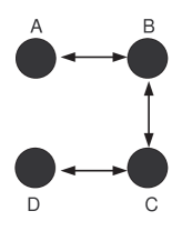
Figure 1: Example of bi-directed graph

The marginal log-linear parameterisation for bi-directed graphs has been proposed by Lupparelli (2006) and Lupparelli et al. (2009); it is based on the class of log-linear marginal models of Bergsma and Rudas (2002). According to Bergsma and Rudas (2002) the parameter vector $\lambda$, containing the marginal log-linear interactions, can be obtained as

$$\mbox{\boldmath$\lambda$}=\mbox{\boldmath$C$}\log\big{(}\mbox{\boldmath$M$}\mbox{\boldmath$P$}\big{)}\mbox{~{}with~{}}\mbox{\boldmath$P$}=\mbox{vec}(\mbox{\boldmath$p$}),$$ (1)

where $\mbox{vec}(\mbox{\boldmath$p$})$ is a vector of dimension $|{\cal I}|$ obtained by rearranging the elements $p$ in a reverse lexicographical ordering of the corresponding variable levels, with the level of the first variable changing first. Each marginal log-linear interaction satisfies identifiability constraints (here sum-to-zero constraints), and this is achieved via an appropriate contrast matrix $C$. The interactions are calculated from a specific marginal table identified via the marginalisation matrix $M$. They are characterised by two sets of variables: one set that refers to the marginal table in use and a second set (subset of the first one) that identifies which variables are involved in the interaction of interest. Finally, the first order interactions correspond to the main effects. We denote with $\mbox{\boldmath$\lambda$}^{M_{m}}$ the parameter vector containing all interactions estimated from the marginal probability table $\mbox{\boldmath$p$}^{M_{m}}$. Matrices $C$ and $M$ define a smooth mapping between the probability space and the marginal log-linear space; see Forcina et al. (2010) for technical details about the smoothness. Matrix $C$ controls the induced log-linear parameterisation. In this work we have used the sum-to-zero parameterisation which is one of the possible configurations leading to different sets of log-linear parameters. Details for the the construction of $C$ and $M$ are available in Appendices B, C and in Section 3.1.

A graphical model of marginal independence is defined by zero constraints on specific marginal log-linear interactions. More precisely, we apply the following procedure presented by Lupparelli (2006) and Lupparelli et al. (2009): (i) define a hierarchical ordering (see Bergsma and Rudas, 2002) of the marginals corresponding to disconnected sets of the bi-directed graph; (ii) append the marginal corresponding to the full table at the end of the list if it is not already included; (iii) for every marginal table estimate all interactions that have not been already obtained from the marginals preceding it in the ordering; (iv) for every marginal table corresponding to a disconnected set of $G$, restrict the highest order log-linear interaction to zero.

The graphical structure imposes constraints of the type

$$\mbox{\boldmath$K$}\log\Big{(}\mbox{\boldmath$M$}\mbox{\boldmath$P$}\Big{)}=0$$

with $K$ being the sub-matrix of $C$ for which the corresponding elements of $\lambda$ are restricted to zero. This parameterisation depends on the ordering of the marginals selected in step (i). Furthermore, it does not always satisfy variation independence; see Lupparelli et al. (2009), Rudas et al. (2010), and Evans and Richardson (2013). If the marginal selected in step (i) are order decomposable then variation independence is guaranteed (Bergsma and Rudas, 2002) so that the marginal-log linear parameter space is rectangular. Hence, in this paper we focus on models based on an order decomposable set of marginals. Graphical log-linear marginal models based on bi-directed graphs with three and four vertices are always variation independent whichever the chosen ordering of the marginals.

3 Bayesian Model Set-up

3.1 Prior Specification for Marginal Log-linear Interactions

In order to specify our prior setting for graphical marginal log-linear models it is useful to rewrite the model described by equation (1) in the following extended form

$$\left(\begin{array}[]{l}\mbox{\boldmath$\lambda$}^{M_{1}}\\ \vdots\\ \mbox{\boldmath$\lambda$}^{M_{m}}\\ \vdots\\ \mbox{\boldmath$\lambda$}^{|\cal{{M}}|}\end{array}\right)=\mbox{diag}\left(\mbox{\boldmath$C$}_{1},\cdots,\mbox{\boldmath$C$}_{m},\cdots,\mbox{\boldmath$C$}_{|{\cal M}|}\right)\left(\begin{array}[]{l}\log\mbox{\boldmath$P$}^{M_{1}}\\ \vdots\\ \log\mbox{\boldmath$P$}^{M_{m}}\\ \vdots\\ \log\mbox{\boldmath$P$}^{|\cal{{M}}|}\end{array}\right),$$ (2)

where ${\cal M}=\{M_{1},\dots,{M_{m}}\dots,M_{|{\cal M}|}\}$ is the set of marginals under consideration, $\mbox{\boldmath$\lambda$}^{M_{m}}$ is the parameter vector obtained from the marginal probability table $\mbox{\boldmath$p$}^{M_{m}}$ which is re-arranged to a vector denoted by $\mbox{\boldmath$P$}^{M_{m}}$ for all $m=1,2,\dots,|{\cal M}|$. The marginals under consideration correspond to the disconnected sets of the graph. If the graph is connected, we need to append the margin that corresponds to the full table to the previous set of marginals. The contrast matrix $C$ is a block diagonal matrix with elements $\mbox{\boldmath$C$}_{m}$. Each sub-matrix $\mbox{\boldmath$C$}_{m}$ is obtained by inverting the design matrix ${\mathbf{X}}_{M_{m}}$ of the saturated model fitted on marginal $M_{m}$, and deleting rows corresponding to interactions that are not estimated from that specific marginal table; see Appendix C for details. From (2), we directly obtain that the interactions $\mbox{\boldmath$\lambda$}^{M_{m}}$ of the marginal $M_{m}$ are obtained by

$$\mbox{\boldmath$\lambda$}^{M_{m}}=\mbox{\boldmath$C$}_{m}\log\mbox{\boldmath$P$}^{M_{m}}\mbox{~{}for all~{}}M_{m}\in{\cal M}.$$

Every $\mbox{\boldmath$\lambda$}^{M_{m}}$ may contain interactions that are constrained to zero due the graphical structure $G$ and the induced contrast matrix. In the following we focus only on non-zero elements of $\lambda$, on which we assign a suitable prior distribution. We denote by $\vec{\mbox{\boldmath$\lambda$}}$ the set of elements of $\lambda$ not restricted to zero, that is

$$\vec{\mbox{\boldmath$\lambda$}} = \left(\vec{\mbox{\boldmath$\lambda$}}^{M_{m}};M_{m}\in{\cal M}\right)\mbox{~{}with~{}}\vec{\mbox{\boldmath$\lambda$}}^{M_{m}}=\left(\lambda^{M_{m}}_{\jmath}:\lambda^{M_{m}}_{\jmath}\neq 0,\jmath=1,\dots,\textsc{r}_{C_{m}}\right),$$

where $\textsc{r}_{C_{m}}$ is the number of rows of the contrast matrix $\mbox{\boldmath$C$}_{m}$ for marginal $M_{m}\in{\cal M}$.

When no information is available about $\vec{\mbox{\boldmath$\lambda$}}$, we can work separately on each element of $\vec{\mbox{\boldmath$\lambda$}}$, assigning suitable independent normal prior distributions with large variance to express ignorance, i.e.

$$f(\vec{\lambda}_{\jmath})\sim N(0,\sigma_{\jmath}^{2})\mbox{ for }\jmath=1,2,\dots,d_{\vec{\lambda}},$$

where $d_{\vec{\lambda}}$ is the number of elements of $\vec{\mbox{\boldmath$\lambda$}}$.

A more sophisticated approach can be based on the prior suggestion of Dellaportas and Forster (1999) for standard log-linear models of the form $\log\mbox{\boldmath$\mu$}=\mbox{\boldmath$X$}\mbox{\boldmath$\beta$}$. They considered the following prior distribution

$$\mbox{\boldmath$\beta$}\sim N\Big{(}\mbox{\boldmath$\theta$},\,2|{\cal I}|\big{(}\mbox{\boldmath$X$}^{T}\mbox{\boldmath$X$}\big{)}^{-1}\Big{)}\mbox{~{}with~{}}\mbox{\boldmath$\theta$}=(\log\overline{\mbox{\boldmath$n$}},\,0,\dots,\,0)^{T},$$ (3)

where $\mu$ is the vector of the expected number of cell frequencies and $|{\cal I}|=\prod\limits_{v\in{\cal V}}\ |{\cal I}_{v}|$ is the number of cells of the contingency table. Matrix $X$ represents the design matrix of the model; see Appendix C for more details and full specification.

This prior was suggested as a default choice for model comparison of log-linear models and it arises naturally for log-linear marginal models since within each marginal we essentially work by fitting standard log-linear models. In fact, following the procedure described in Section 2, for every marginal we fit a saturated log-linear model, and then we keep only interactions that have not been already estimated from the marginal preceding it in the examined ordering.

Dellaportas and Foster prior was obtained after matching the prior moments of other default priors used for the probability parameters in conjugate analysis of graphical models such as the Jeffreys and the Perks prior distributions, for more details see Sections 3.2 and 3.3 in Dellaportas and Forster (1999). Moreover, the prior distribution induced for the log-odds ratios remains the same even if extra, marginally independent, categorical variables are added in the model. Finally, such prior arises naturally in our context since the adopted parameterisation allows us to work by fitting standard log-linear models within each marginal. These are the main reasons why we recommend adopting this prior here.

The prior mean vector $\theta$ has all its elements equal to zero except the first one which is equal to the logarithm of the average number of observations per cell $\overline{\mbox{\boldmath$n$}}$. Under sum-to-zero constraints, $\mbox{\boldmath$X$}^{T}\mbox{\boldmath$X$}$ is a block diagonal matrix resulting to a set of independent priors for interactions referring to different set of variables.

In order to construct the prior distribution on $\vec{\mbox{\boldmath$\lambda$}}$, we work separately on each single set ${\mbox{\boldmath$\lambda$}}^{M_{m}}$ obtained from marginal $M_{m}$ and we proceed as follows. Let $\mbox{\boldmath$\lambda$}^{M_{m}}_{S}$ be the parameter vector for the saturated model that can be estimated from marginal $M_{m}$; by construction, it coincides with the parameter vector of the saturated standard log-linear model obtained from this marginal. In terms of Dellaportas and Forster (1999) parameterisation, $\mbox{\boldmath$\lambda$}^{M_{m}}_{S}$ can be written as $\mbox{\boldmath$\lambda$}^{M_{m}}_{S}=\mbox{\boldmath$\beta$}^{M_{m}}-\log(N)\,{\mathbf{X}}_{M_{m}}^{-1}\mbox{\boldmath$1$}$. Hence, from (3), the default prior for $\mbox{\boldmath$\lambda$}^{M_{m}}_{S}$ is given by

$$\mbox{\boldmath$\lambda$}^{M_{m}}_{S}\sim N\Big{(}\mbox{\boldmath$\theta$}-\log(N)\,{\mathbf{X}}_{M_{m}}^{-1}\mbox{\boldmath$1$}\;,\;2|{\cal I}_{M_{m}}|\left(\mbox{\boldmath$X$}_{M_{m}}^{T}\mbox{\boldmath$X$}_{M_{m}}\right)^{-1}\Big{)}.$$ (4)

The prior of $\vec{\mbox{\boldmath$\lambda$}}^{M_{m}}$ is obtained via marginalisation from (4) since $\vec{\mbox{\boldmath$\lambda$}}^{M_{m}}$ is a subset of $\mbox{\boldmath$\lambda$}^{M_{m}}_{S}$. When using sum-to-zero constraints, then $\mbox{\boldmath$X$}_{M_{m}}^{-1}\mbox{\boldmath$1$}=(1,0,\dots,0)^{T}$ resulting to a prior mean equal to $\theta_{\jmath}=0$ for all $\vec{\mbox{\boldmath$\lambda$}}^{M_{m}}_{\jmath}$ except for the intercept for which the prior mean is given by $\log\overline{\mbox{\boldmath$n$}}-\log(N)$. This prior is greatly simplified to a product of independent $N(0,2)$ for all marginal log-linear interactions (except for the intercept) in the case of binary variables. Finally, the prior for the full parameter vector $\vec{\mbox{\boldmath$\lambda$}}$ is obtained as a product of the priors on $\vec{\mbox{\boldmath$\lambda$}}^{M_{m}}$.

3.2 Likelihood Specification and Posterior Inference

The likelihood cannot directly be expressed in terms of $\lambda$ (or equivalently $\vec{\mbox{\boldmath$\lambda$}}$) but only as a function of the probability parameter

$$f(\mbox{\boldmath$n$}|\mbox{\boldmath$\lambda$}) = \frac{\Gamma(N+1)}{\prod\limits_{i\in{\cal I}}\Gamma\big{(}n(i)+1\big{)}}\prod_{i\in{\cal I}}\wp_{i}(\mbox{\boldmath$\lambda$})^{n(i)},$$

$$\mbox{where\;}\wp_{i}(\mbox{\boldmath$\lambda$}) \equiv \left\{p(i):\mbox{\boldmath$\lambda$}=\mbox{\boldmath$C$}\log\Big{(}\mbox{\boldmath$M$}\mbox{\boldmath$P$}\Big{)}\right\},\mbox{~{}for all~{}}i\in{\cal I}~{}.$$ (5)

Unfortunately, in order to obtain $\wp_{i}(\mbox{\boldmath$\lambda$})$, or equivalently $P$, from (1), we need to implement an iterative algorithm, and therefore the likelihood cannot be written in a closed form expression, see, for example, Bergsma and Rudas (2002), and Lupparelli et al. (2009). As a consequence of this, the corresponding posterior distribution of $\lambda$ (or equivalently $\vec{\mbox{\boldmath$\lambda$}}$), cannot be evaluated straight away. Hence, MCMC methods are needed for posterior inference of $\vec{\mbox{\boldmath$\lambda$}}$.

Metropolis-Hastings scheme on the marginal log-linear interactions can be implemented to estimate the posterior distributions of the parameter vector. Nevertheless, such an algorithmic strategy will be inefficient since in every MCMC iteration, the joint probabilities corresponding to the proposed values of $\lambda$ need to be calculated using an iterative algorithm. This will considerably slow down the MCMC sampler. The use of the iterative procedure may also result to unstable solutions for specific combinations of lambda values. During simulations we have encountered several inconsistencies in the estimates for specific configurations that may have unpredicted effect on the MCMC runs and the corresponding estimated posterior distributions. Another important issue is the fact that the constructed algorithm should generate parameter values that lead to well-defined joint probability distributions with compatible marginals. Defining a proposal distribution that allows moving within the space of variation independent log-linear marginal models is still an open issue.

For the above reasons, in the following section, we propose a novel MCMC strategy based on the probability representation of the model. Such probabilities are compatible by construction, the corresponding marginal log-linear interactions will be also compatible. For comparative purposes, we have implemented a “vanilla” random walk algorithm MCMC on $\vec{\mbox{\boldmath$\lambda$}}$ (referred to as RW-$\lambda$), which proposes to change each log-linear parameter vector independently for every single marginal based on a decomposable ordering.

4 Probability Based MCMC Samplers

4.1 Initial Set-up and Data Augmentation for MCMC

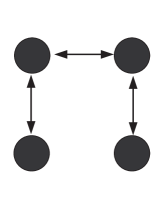
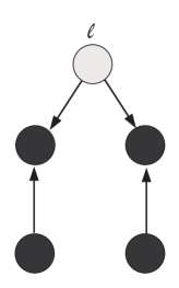
Figure 2: Bi-directed 4-chain graph and the corresponding Markov equivalent DAG over the observed margin.

Following the notation of Ntzoufras and Tarantola (2013), we can divide the class of graphical log-linear marginal models in two major categories: homogeneous and non-homogeneous models. A bi-directed graph is named homogeneous if it does not include a bi-directed 4-chain or a chordless 4-cycle as sub-graphs. Both type of models are shown to be compatible, in terms of independencies, with a certain DAG representation (augmented DAG); see Pearl and Wermuth (1994), Drton and Richardson (2008) and Silva and Ghahramani (2009a, b). Nevertheless, while homogeneous models can be generated via a DAG with the same vertex set, for the non-homogeneous ones it is necessary to include some additional latent variables which makes Bayesian inference challenging. The advantage of the augmented DAG representation is that the joint probability over the augmented variable space (including both observed and latent variables) can be written using the standard DAG factorisation. An example of the DAG representation with latent variables for a non-homogeneous bi-directed graph is provided in Figure 2.

In order to construct the augmented DAG, with the minimal set of latent variables, we apply the following procedure presented in Pearl and Wermuth (1994). Given the skeleton $\overline{G}$ of the examined graph, we assign arrows $v_{\imath}\longrightarrow v_{\jmath}\longleftarrow v_{k}$ to each $\vee$ configuration $(v_{\imath},v_{\jmath},v_{k})$ in $\overline{G}$, constructing in this way the sink orientation of $G$. If no edge in the sink orientation is bi-directed we consider an acyclic orientation of the undirected edges. If the sink orientation contains bi-directed edges, we substitute every bi-directed edge $v_{1}\longleftrightarrow v_{2}$ with the directed configuration $v_{1}\longleftarrow\ell\longrightarrow v_{2}$, where vertex $\ell$ represents a hidden or latent variable. Finally, a DAG is constructed via an acyclic orientation of the undirected edges which are present in the sink orientation of the graph. Any DAG which encodes the same independencies between the observable variables as in $G$ is called augmented DAG of $G$.

Ntzoufras and Tarantola (2013) exploited the connection between bi-directed graphs and DAGs to develop a Gibbs sampler based on a probability parameterisation of the model. They parameterised the augmented DAG model in terms of a set of marginal and conditional probability parameters $\Pi$, on which they implemented a conjugate analysis based on products of Dirichlet distributions. For homogeneous bi-directed graphs, the posterior distribution of the probability vector for the observed variables can be obtained analytically. On the other hand, for non-homogenous graphs, a Gibbs sampler can be obtained by calculating appropriate contrasts of the logarithms of the probability parameters within the proposed data augmentation scheme. The Gibbs sampler for the non-homogenous models is essentially composed by three steps:

Step 1:

Generate random splits for each bi-directed edge in the sink orientation of $G$ by using a multinomial distribution (i.e. we generate the latent data).

Step 2:

Generate random samples from the induced Dirichlet posterior conditional distributions for each set of probability parameters of the augmented DAG, given the augmented table of Step 1.

Step 3:

Calculate the joint and the marginal probabilities for the observed variables by implementing the appropriate marginalising transformations to the probability parameter values of Step 2.

Additionally, the posterior distribution of the log-linear interactions can be obtained as by-product of this approach. This can be achieved by calculating appropriate contrasts of the logarithms of the joint probability parameters obtained in Step 3. We may implement this by either adding an additional step to the above algorithm or by implementing the induced transformation on the final MCMC output of the algorithm.

However this approach is open to the following critics. First of all, prior information is usually available about the marginal association of the observed variables. This is typically expressed by the size of log-linear interactions which correspond to log-odds. Any prior information available for log-odds cannot be incorporated in a probability based method in a trivial manner. For instance, symmetry constraints, context specific independence assumptions, vanishing high-order associations or further prior information about the joint and marginal distributions can be specified by setting zero or linear constraints on the marginal log-linear parameter space, instead of non-linear multiplicative constraints on the probability space. Specifying sub-models based on a priori knowledge is an important issue for discrete bi-directed graph models. In fact, they generally require to extimate a higher number of parameters compared to models of conditional independencies, such as undirected graph and DAG models; see Lupparelli et al. (2009) for a discussion which compares the number of parameters in discrete bi-directed and undirected graph models with the same skeleton. From this perspective, the marginal log-linear parameterisation is definitively more appealing than the probability based approach.

In this paper, we introduce a novel MCMC strategy, in which the model and the prior are expressed in terms of the marginal log-linear interactions, while the proposal is defined on the probability parameter space. By this way, we can incorporate any source of prior information that might be available regarding marginal associations by specifying the prior values of selected log-odds ratios (i.e. interactions). Moreover, we can exploit the advantages of the conditional conjugacy of the algorithm of Ntzoufras and Tarantola (2013) in order to obtain efficient proposals based on probability parameters. This approach allows us to control the induced values and constraints on interactions in the log-linear space in more natural way than working in the probability space induced by the (augmented) DAG.

Our approach does not account for any additional non-independence constraints which may arise by marginalising the latent variables from the augmented DAGs. Defining the exact class of marginal DAGs still represents an open issue; see Evans (2016) who discusses possible approximations. Moreover, these inequality constraints are not of great interest as they do not have a straightforward interpretation. Finally, it is worth noting that if non-independence constraints are included after marginalising over the latent variable, the resulting likelihood is a close approximation of the true one.

(a) Bi-directed graph	(b) DAG representation

Using the methodology of Ntzoufras and Tarantola (2013), we construct an MCMC sampler based on proposing values in terms of joint probabilities, avoiding compatibility problems. If the model is homogeneous the dimension of $\Pi$ is the same as the dimension of $\vec{\mbox{\boldmath$\lambda$}}$. This is not true for non-homogeneous models since the dimension of $\Pi$ is greater than the dimension of $\vec{\mbox{\boldmath$\lambda$}}$. In this case we need to augment the parameter space in order to implement Metropolis-Hastings algorithm. In the following, we denote the augmented set of marginal log-linear interactions by with $\mbox{\boldmath$\lambda$}^{\cal A}$. If the model is homogeneous, then $\mbox{\boldmath$\lambda$}^{\cal A}=\vec{\mbox{\boldmath$\lambda$}}$. Otherwise, we set $\mbox{\boldmath$\lambda$}^{\cal A}=(\vec{\mbox{\boldmath$\lambda$}},\mbox{\boldmath$\xi$})$; where $\xi$ is selected to be the last $d_{\xi}$ elements of $\mbox{\boldmath$\lambda$}^{\cal A}$ with $d_{\xi}=\dim(\mbox{\boldmath$\Pi$})-\dim(\vec{\mbox{\boldmath$\lambda$}})$. The vector $\xi$ can be thought as an auxiliary set of parameters which are used to retain the dimension balance in the Metropolis-Hastings algorithm.

More precisely, for any graphical log-linear marginal model $G$ we can obtain a Markov equivalent DAG over the observed margins, denoted by $D_{G}$, with augmented vertex set ${\cal A}=\{{\cal V},{\cal L}\}$, where ${\cal L}$ is the set of additional latent variables; if $G$ is homogeneous then ${\cal L}=\emptyset$ and ${\cal A}={\cal V}$. Under this approach, the joint probabilities can be written as

$$p(i)=\sum_{i_{\cal L}\in{\cal I}_{\cal L}}p^{{\cal A}}(i,i_{\cal L})\mbox{~{}for~{}}i\in{\cal I}_{\cal V},$$ (6)

$$p^{{\cal A}}(i,i_{\cal L})=p^{{\cal A}}(i^{*})=\prod_{v\in\mathcal{A}}\pi_{v|pa(v)}\left(i^{*}_{v}|i^{*}_{pa(v)}\right)\mbox{~{}for~{}}i^{*}=(i,i_{\cal L})\in{\cal I}_{\cal A},$$ (7)

and the probability parameter set is given by

$$\mbox{\boldmath$\Pi$}=\mbox{vec}\Big{(}{\pi}_{v|pa(v)}(i^{*}_{v}|i^{*}_{pa(v)});\,i^{*}_{v}\in{\cal I}_{v}\setminus\Big{\{}|{\cal I}_{v}|\Big{\}},i^{*}_{pa(v)}\in{\cal I}_{pa(v)},v\in{\cal A}\Big{)},$$

where $p^{{\cal A}}(i^{*})=P\big{(}Y_{\cal V}=i^{*}_{\cal V},Y_{\cal L}=i^{*}_{\cal L}\big{)}$ is the joint probability for the observed variables $Y_{\cal V}$ and the latent variables $Y_{\cal L}$, $pa(v)$ stands for the parents set of $v$ in graph $D_{G}$, $\pi_{v|pa(v)}\big{(}i^{*}_{v}|i^{*}_{pa(v)}\big{)}=P\big{(}Y_{v}=i^{*}_{v}|Y_{pa(v)}=i^{*}_{pa(v)}\big{)}$ is the conditional probability of each variable $Y_{v}$ given variables $Y_{pa(v)}$ in the parent set $pa(v)$ of $v$. By using the induced augmented likelihood representation, we are able to construct a Gibbs sampler based on the conditional conjugate Dirichlet prior distributions on $\Pi$ (Ntzoufras and Tarantola, 2013).

4.2 The general algorithm

The posterior distribution of the augmented set of marginal log-linear interactions is given by

$$f({\mbox{\boldmath$\lambda$}}^{\cal A}|\mbox{\boldmath$n$}) \propto f\Big{(}\mbox{\boldmath$n$}|{\mathbf{\wp}}({\mbox{\boldmath$\lambda$}})\Big{)}f(\vec{\mbox{\boldmath$\lambda$}})f(\mbox{\boldmath$\xi$}),$$

where $f(\mbox{\boldmath$\xi$})$ is a pseudo prior used for the additional parameters.

We consider a Metropolis-Hastings algorithm which can be summarised by the following steps.

1. For $t=1,\dots,T$, repeat the following steps:

2. Propose a new vector $\mbox{\boldmath$\Pi$}^{\prime}$ from $q(\mbox{\boldmath$\Pi$}^{\prime}|\mbox{\boldmath$\Pi$}^{(t)})$; where $\mbox{\boldmath$\Pi$}^{(t)}$ are the values of $\Pi$ at $t$ iteration.

3. From $\mbox{\boldmath$\Pi$}^{\prime}$, calculate the proposed joint probabilities $\mbox{\boldmath$p$}^{\prime}$ (for the observed table) using equations (6) and (7).

4. From $\mbox{\boldmath$p$}^{\prime}$, calculate ${\mbox{\boldmath$\lambda$}}\,\!^{\prime}$ using (1) and then obtain the corresponding non-zero elements $\vec{\mbox{\boldmath$\lambda$}}\,\!^{\prime}$.

5. Set $\mbox{\boldmath$\xi$}^{\prime}=\mbox{\boldmath$\Pi$}_{\xi}^{\prime}$; where $\mbox{\boldmath$\Pi$}_{\xi}^{\prime}$ is a pre-specified subset of $\mbox{\boldmath$\Pi$}^{\prime}$ of dimension $d_{\xi}=\dim(\mbox{\boldmath$\Pi$})-\dim(\vec{\mbox{\boldmath$\lambda$}})$; in our implementation we have used as $\xi$ the last $d_{\xi}$ terms of $\mbox{\boldmath$\Pi$}_{\xi}$.

6. Accept the proposed move with probability $\alpha=\min(1,A)$ with

   $$A = \frac{f\Big{(}\mbox{\boldmath$n$}|{\mathbf{\wp}}\big{(}\mbox{\boldmath$\lambda$}\,\!^{\prime}\big{)}\Big{)}f\big{(}\vec{\mbox{\boldmath$\lambda$}}\,\!^{\prime}\big{)}f\left(\mbox{\boldmath$\xi$}^{\prime}\right)q\big{(}\vec{\mbox{\boldmath$\lambda$}}\,\!^{(t)},\,\mbox{\boldmath$\xi$}^{(t)}\big{|}\vec{\mbox{\boldmath$\lambda$}}\,\!^{\prime},\,\mbox{\boldmath$\xi$}^{\prime}\big{)}}{f\Big{(}\mbox{\boldmath$n$}|{\mathbf{\wp}}\big{(}\mbox{\boldmath$\lambda$}^{(t)}\big{)}\Big{)}f\big{(}\vec{\mbox{\boldmath$\lambda$}}\,\!^{(t)}\big{)}f(\mbox{\boldmath$\xi$}^{(t)})q\big{(}\vec{\mbox{\boldmath$\lambda$}}\,\!^{\prime},\,\mbox{\boldmath$\xi$}^{\prime}\big{|}\vec{\mbox{\boldmath$\lambda$}}\,\!^{(t)},\,\mbox{\boldmath$\xi$}^{(t)}\big{)}}$$ (8)

   $$= \frac{f(\mbox{\boldmath$n$}|\mbox{\boldmath$\Pi$}^{\prime})f\big{(}\vec{\mbox{\boldmath$\lambda$}}\,\!^{\prime}\big{)}f(\mbox{\boldmath$\xi$}^{\prime})q(\mbox{\boldmath$\Pi$}^{(t)}|\mbox{\boldmath$\Pi$}^{\prime})}{f(\mbox{\boldmath$n$}|\mbox{\boldmath$\Pi$}^{(t)})f\big{(}\vec{\mbox{\boldmath$\lambda$}}\,\!^{(t)}\big{)}f(\mbox{\boldmath$\xi$})q(\mbox{\boldmath$\Pi$}^{\prime}|\mbox{\boldmath$\Pi$}^{(t)})}\times\mbox{abs}\left(\frac{{\cal J}\Big{(}\mbox{\boldmath$\Pi$}^{(t)},\vec{\mbox{\boldmath$\lambda$}}\,\!^{(t)},\mbox{\boldmath$\xi$}^{(t)}\Big{)}}{{\cal J}\Big{(}\mbox{\boldmath$\Pi$}^{\prime},\vec{\mbox{\boldmath$\lambda$}}\,\!^{\prime},\mbox{\boldmath$\xi$}^{\prime}\Big{)}}\right),$$

   where $\mbox{abs}(\cdot)$ stands for the absolute value, $\mbox{\boldmath$\Pi$}_{\xi}=\mbox{\boldmath$\xi$}$, and ${\cal J}={\cal J}(\mbox{\boldmath$\Pi$},\vec{\mbox{\boldmath$\lambda$}},\mbox{\boldmath$\xi$})$ is the determinant of the Jacobian matrix of the transformation $\mbox{\boldmath$\Pi$}=g(\vec{\mbox{\boldmath$\lambda$}},\mbox{\boldmath$\xi$})$ specified by Equations (6), (7), and (1). Similarly to Step 1, $\vec{\mbox{\boldmath$\lambda$}}\,\!^{(t)}$, $\mbox{\boldmath$\xi$}^{(t)}$ and $\mbox{\boldmath$\lambda$}^{(t)}$ are used to denote the values of the corresponding parameters in the current iteration $t$ of the algorithm.

7. If the move is accepted, then set $\mbox{\boldmath$\Pi$}^{(t+1)}=\mbox{\boldmath$\Pi$}^{\prime}$, $\mbox{\boldmath$\xi$}^{(t+1)}=\mbox{\boldmath$\xi$}^{\prime}$, and $\vec{\mbox{\boldmath$\lambda$}}^{(t+1)}=\vec{\mbox{\boldmath$\lambda$}}\,\!^{\prime}$ otherwise set $\mbox{\boldmath$\Pi$}^{(t+1)}=\mbox{\boldmath$\Pi$}^{(t)}$ and $\vec{\mbox{\boldmath$\lambda$}}^{(t+1)}=\vec{\mbox{\boldmath$\lambda$}}^{(t)}$.

The pseudo-parameter vector $\xi$ is used only to retain the dimension balance between the marginal log-linear parameterisation and the probability parameterisation used in Ntzoufras and Tarantola (2013). Furthermore, it is directly matched to specific probability parameters of the bi-directed graph $G$. Hence, we can indirectly “eliminate” the effects of $\xi$ on the algorithm by assuming that its elements are uniformly distributed in the zero-one interval. Under this view, we set $f(\xi_{\imath})=I_{\{0<\xi_{\imath}<1\}}$ having as a result the elimination of the ratio $f(\mbox{\boldmath$\xi$}^{\prime})/f(\mbox{\boldmath$\xi$}^{(t)})$ from (8). In the following, we consider this choice in order to simplify all proposed algorithms.

A good choice of the proposal $q(\mbox{\boldmath$\Pi$}^{\prime}|\mbox{\boldmath$\Pi$}^{(t)})$ will lead to high (close to one) acceptance rates. Therefore, an efficient proposal for the Metropolis Hastings scheme described in this section, intuitively seems to be the following

$$q(\mbox{\boldmath$\Pi$}^{\prime}|\mbox{\boldmath$\Pi$}^{(t)})=\sum_{n_{\cal A}}f_{q}\big{(}\mbox{\boldmath$\Pi$}^{\prime}|\mbox{\boldmath$n$}^{\prime\cal A}\big{)}f\big{(}\mbox{\boldmath$n$}^{\prime\cal A}|\mbox{\boldmath$\Pi$}^{(t)},\mbox{\boldmath$n$}\big{)},$$ (9)

where $f\big{(}\mbox{\boldmath$n$}^{\cal A}|\mbox{\boldmath$\Pi$},\mbox{\boldmath$n$}\big{)}$ is the distribution of counts $\mbox{\boldmath$n$}^{\cal A}$ given the observed frequency table $n$ and the probability parameter set $\Pi$ of the augmented table induced by ${\cal A}$; and $f_{q}\big{(}\mbox{\boldmath$\Pi$}|\mbox{\boldmath$n$}^{\cal A}\big{)}$ is the conditional posterior distribution of the probability parameter vector $\Pi$ given a proposed set of augmented data $\mbox{\boldmath$n$}^{{\cal A}}$. Considering all possible configurations in (9) within each MCMC iteration is cumbersome and time-consuming. One solution can be obtained by using a random sub-sample of $\mbox{\boldmath$n$}^{{\cal A}}$. Hence, we construct our MCMC by employing just one realisation of $\mbox{\boldmath$n$}^{\cal A}$ which will play the role of intermediate nuisance parameter that facilitates the construction of a sensible proposal distribution. This approach corresponds to an MCMC scheme with a target posterior distribution given by

$$f({\mbox{\boldmath$\lambda$}}^{\cal A},\mbox{\boldmath$n$}^{\cal A}|\mbox{\boldmath$n$}) \propto f\big{(}\mbox{\boldmath$n$}|{\mathbf{\wp}}({\mbox{\boldmath$\lambda$}})\big{)}f(\vec{\mbox{\boldmath$\lambda$}})f(\mbox{\boldmath$\xi$})f(\mbox{\boldmath$n$}^{\cal A}).$$

The parameter vector $\mbox{\boldmath$n$}^{\cal A}$ plays the role of (nuisance) augmented data with $f(\mbox{\boldmath$n$}^{\cal A})$ being a pseudo-prior. More precisely, we introduce $\mbox{\boldmath$n$}^{\cal A}$ in order to augment the target posterior and to achieve a dimension balance between the two parameterizations: the marginal log-linear parameterisation and the probability based one. This trick assists us to retain the balance between the two parametrisations and it enables us to implement standard MCMC methods.

In order to simplify the MCMC configuration, we consider a uniform distribution as pseudo-prior over all possible configurations of $\mbox{\boldmath$n$}^{\cal A}$. Under this formulation, the acceptance probability in the Metropolis-Hastings is equal to $\alpha=\min(1,A)$ with $A$ given by

$$A = \frac{f\big{(}\mbox{\boldmath$n$}|\mbox{\boldmath$\Pi$}^{\prime}\big{)}f\big{(}\vec{\mbox{\boldmath$\lambda$}}\,\!^{\prime}\big{)}f_{q}\big{(}\mbox{\boldmath$\Pi$}^{(t)}|\mbox{\boldmath$n$}^{{\cal A}(t)}\big{)}f\big{(}\mbox{\boldmath$n$}^{{\cal A}(t)}|\mbox{\boldmath$\Pi$}^{\prime},\mbox{\boldmath$n$}\big{)}}{f\big{(}\mbox{\boldmath$n$}|\mbox{\boldmath$\Pi$}^{(t)}\big{)}f\big{(}\vec{\mbox{\boldmath$\lambda$}}\,\!^{(t)}\big{)}f_{q}\big{(}\mbox{\boldmath$\Pi$}^{\prime}|\mbox{\boldmath$n$}^{\prime\cal A}\big{)}f\big{(}\mbox{\boldmath$n$}^{\prime\cal A}|\mbox{\boldmath$\Pi$}^{(t)},\mbox{\boldmath$n$}\big{)}}\times\mbox{abs}\left(\frac{{\cal J}\big{(}\mbox{\boldmath$\Pi$}^{(t)},\vec{\mbox{\boldmath$\lambda$}}\,\!^{(t)},\mbox{\boldmath$\xi$}^{(t)}\big{)}}{{\cal J}\big{(}\mbox{\boldmath$\Pi$}^{\prime},\vec{\mbox{\boldmath$\lambda$}}\,\!^{\prime},\mbox{\boldmath$\xi$}^{\prime}\big{)}}\right).$$ (10)

In (10), the probability functions $f\big{(}\mbox{\boldmath$n$}^{\prime\cal A}|\mbox{\boldmath$\Pi$},\mbox{\boldmath$n$}\big{)}$ and $f\big{(}\mbox{\boldmath$n$}^{{\cal A}(t)}|\mbox{\boldmath$\Pi$}^{\prime},\mbox{\boldmath$n$}\big{)}$ are readily available from the model construction and the likelihood representation of the augmented table. We only need to specify $f_{q}\big{(}\mbox{\boldmath$\Pi$}^{\prime}|\mbox{\boldmath$n$}^{\prime\cal A}\big{)}$ which is the first component of (9) and it has the form of a posterior conditionally on the frequencies of the augmented table. For this component, we can exploit the conditional conjugate approach of Ntzoufras and Tarantola (2013). In order to do so, we consider as a “prior” $f_{q}(\mbox{\boldmath$\Pi$})$ a product of Dirichlet distributions in order to obtain a conjugate “posterior” distribution $f_{q}(\mbox{\boldmath$\Pi$}^{\prime}|\mbox{\boldmath$n$}^{\prime\cal A})$. Under this approach, and by further considering that $f\big{(}\mbox{\boldmath$n$}|\mbox{\boldmath$\Pi$}\big{)}f\big{(}\mbox{\boldmath$n$}^{\cal A}|\mbox{\boldmath$\Pi$},\mbox{\boldmath$n$}\big{)}=f\big{(}\mbox{\boldmath$n$}^{\cal A}|\mbox{\boldmath$\Pi$}\big{)}$, then (10) is further simplified to

$$A = \frac{f\big{(}\mbox{\boldmath$n$}^{{\cal A}(t)}|\mbox{\boldmath$\Pi$}^{\prime}\big{)}f\big{(}\vec{\mbox{\boldmath$\lambda$}}\,\!^{\prime}\big{)}f_{q}\big{(}\mbox{\boldmath$\Pi$}^{(t)}|\mbox{\boldmath$n$}^{{\cal A}(t)}\big{)}}{f\big{(}\mbox{\boldmath$n$}^{\prime\cal A}|\mbox{\boldmath$\Pi$}^{(t)}\big{)}f\big{(}\vec{\mbox{\boldmath$\lambda$}}\,\!^{(t)}\big{)}f_{q}\big{(}\mbox{\boldmath$\Pi$}^{\prime}|\mbox{\boldmath$n$}^{\prime\cal A}\big{)}}\times\mbox{abs}\left(\frac{{\cal J}\big{(}\mbox{\boldmath$\Pi$}^{(t)},\vec{\mbox{\boldmath$\lambda$}}\,\!^{(t)},\mbox{\boldmath$\xi$}^{(t)}\big{)}}{{\cal J}\big{(}\mbox{\boldmath$\Pi$}^{\prime},\vec{\mbox{\boldmath$\lambda$}}\,\!^{\prime},\mbox{\boldmath$\xi$}^{\prime}\big{)}}\right)\,.$$ (11)

In the following of this manuscript, we will refer to this approach as the probability-based independence sampler (PBIS).

4.3 Prior Adjustment Algorithm

As we have already stated, although PBIS simplifies the MCMC scheme, the parameter space is still considerably extended by considering the augmented frequency table $\mbox{\boldmath$n$}^{\cal A}$. We can further simplify PBIS by using the following two-step procedure:

     Step 1:

Run the Gibbs sampler of Ntzoufras and Tarantola (2013) to obtain a sample from $\Pi$ (see Section 4.1 for more details).

     Step 2:

Use the sample of step 1 (or sub-sample of it) as a proposal in the general Metropolis-Hastings algorithm with acceptance rate (8).

Since the sample of Step 1 is obtained from an MCMC algorithm, auto-correlation will be present. A random (independent) sub-sample from the posterior distribution can be obtained by following different strategies. The most common approach can be obtained by using thinning, where we keep one observation for every set of $K$ iterations. The thinning interval $K$ can be easily defined by monitoring autocorrelation function or using the convergence diagnostic of Raftery and Lewis (1992) which is available in R packages such as CODA or BOA. A drawback of this approach is that we may end up having a considerably lower number of simulated observations. For this reason, we suggest considering a random permutation of the full MCMC sample to “destroy” the induced autocorrelation. We believe that the effect of this strategy will be minimal, since this sample is only used as a proposal in the second MCMC procedure. As a referee pointed out, by following either of these approaches, the sample variance will get close to the independent variance asymptotically. Although intuitively this approach will lead to a sample from the target posterior distribution (or a close approximation of it), to our knowledge no mathematical proof is available. Indeed, empirical comparisons (see Section 5.1) indicate no differences between the posterior distribution obtained by a correctly thinned MCMC sample and the re-ordered sample or even with the one-shot MCMC sampler of Section 4.2. Therefore, we believe that this sampler provides an efficient approximation of an independence Metropolis-Hastings algorithm.

Using such sample (or sub-sample) as proposed values within the Metropolis-Hasting algorithm is equivalent to using the posterior distribution $f_{q}(\mbox{\boldmath$\Pi$}|\mbox{\boldmath$n$})$ as proposal in (8), that is $q(\mbox{\boldmath$\Pi$}^{\prime}|\mbox{\boldmath$\Pi$}^{(t)})=f_{q}(\mbox{\boldmath$\Pi$}^{\prime}|\mbox{\boldmath$n$}).$ Under this proposal, (8) now simplifies to

$$A = \frac{f(\vec{\mbox{\boldmath$\lambda$}}\,\!^{\prime})f_{q}(\mbox{\boldmath$\Pi$}^{(t)})}{f(\vec{\mbox{\boldmath$\lambda$}}\,\!^{(t)})f_{q}(\mbox{\boldmath$\Pi$}^{\prime})}\times\mbox{abs}\left(\frac{{\cal J}\Big{(}\mbox{\boldmath$\Pi$}^{(t)},\vec{\mbox{\boldmath$\lambda$}}\,\!^{(t)},\mbox{\boldmath$\xi$}^{(t)}\Big{)}}{{\cal J}\Big{(}\mbox{\boldmath$\Pi$}^{\prime},\vec{\mbox{\boldmath$\lambda$}}\,\!^{\prime},\mbox{\boldmath$\xi$}^{\prime}\Big{)}}\right).$$ (12)

We will refer to this algorithm as the prior-adjustment algorithm (PAA) due to its characteristic to correct for the differences between the prior distributions used under the two parameterisations.

The “prior” distribution $f_{q}(\mbox{\boldmath$\Pi$})$ is only used to build the proposal. Therefore, it can be considered as a pseudo-prior. It does not influence the target posterior distribution but only affects the convergence rates of PAA. We can choose the parameters of this pseudo-prior in such a way that (12) is maximized and an optimal acceptance rate is achieved. When a non-informative prior distribution for $\vec{\mbox{\boldmath$\lambda$}}$ is used, all Dirichlet parameters involved in $f_{q}(\mbox{\boldmath$\Pi$})$ can be set equal to one. Under this choice, the effect of the pseudo-prior is eliminated from the proposal, leaving the data-likelihood to guide the MCMC algorithm. PAA is less computationally demanding that the single-run MCMC algorithm introduced in Section 4.2, since in we avoid four additional likelihood evaluations at each iteration required in the later.

4.4 The Jacobian

We conclude this section by providing analytical expressions of the Jacobian required in the acceptance probabilities within each MCMC step in Sections 4.2 and 4.3; see Equations (11) and (12). Specifically, the Jacobian terms are given by ${\cal J}(\mbox{\boldmath$\Pi$},\vec{\mbox{\boldmath$\lambda$}},\mbox{\boldmath$\xi$})=\left|\dfrac{\partial\mbox{\boldmath$\Pi$}}{\partial(\vec{\mbox{\boldmath$\lambda$}},\mbox{\boldmath$\xi$})}\right|$ and are simplified to

$${\cal J}^{-1}=\left|\dfrac{\partial(\vec{\mbox{\boldmath$\lambda$}},\mbox{\boldmath$\xi$})}{\partial\mbox{\boldmath$\Pi$}}\right|=\left|\dfrac{\partial(\vec{\mbox{\boldmath$\lambda$}},\mbox{\boldmath$\xi$})}{\partial(\mbox{\boldmath$\Pi$}_{\xi},\mbox{\boldmath$\Pi$}_{\setminus\xi})}\right| = \left|\begin{matrix}\dfrac{\partial\vec{\mbox{\boldmath$\lambda$}}}{\partial\mbox{\boldmath$\Pi$}_{\xi}}&\dfrac{\partial\vec{\mbox{\boldmath$\lambda$}}}{\partial\mbox{\boldmath$\Pi$}_{\setminus\xi}}\\ \dfrac{\partial\mbox{\boldmath$\xi$}}{\partial\mbox{\boldmath$\Pi$}_{\xi}}&\dfrac{\partial\mbox{\boldmath$\xi$}}{\partial\mbox{\boldmath$\Pi$}_{\setminus\xi}}\end{matrix}\right|$$

$$= \left|\begin{matrix}\dfrac{\partial\vec{\mbox{\boldmath$\lambda$}}}{\partial\mbox{\boldmath$\Pi$}_{\xi}}&\dfrac{\partial\vec{\mbox{\boldmath$\lambda$}}}{\partial\mbox{\boldmath$\Pi$}_{\setminus\xi}}\\ \mbox{\boldmath$I$}&\mbox{\boldmath$0$}\end{matrix}\right|=-\left|\begin{matrix}\dfrac{\partial\vec{\mbox{\boldmath$\lambda$}}}{\partial\mbox{\boldmath$\Pi$}_{\setminus\xi}}\end{matrix}\right|,$$

where $\mbox{\boldmath$\Pi$}_{\setminus\xi}$ is obtained from $\Pi$ excluding the elements of $\mbox{\boldmath$\Pi$}_{\xi}$.

The elements of the Jacobian matrix are given by

$$\frac{\partial\lambda_{k}}{\partial\Pi_{\jmath}}=\sum_{l=1}^{\textsc{c}_{C}}\left\{C_{kl}\left(\sum_{\imath=1}^{|{\cal I}|}M_{l\imath}P_{\imath}\right)^{-1}\sum\limits_{\imath=1}^{|{\cal I}|}M_{l\imath}\Delta_{\imath\jmath}\right\}\mbox{~{}with~{}}\Delta_{\imath\jmath}=\frac{\partial P_{\imath}}{\partial\Pi_{\jmath}},$$ (13)

where ${P}_{\imath}$ denote the $\imath$ element of $P$, and $\textsc{c}_{C}$ is the number of columns of the contrast matrix $C$. For the saturated model, the above equation simplifies to

$$\frac{\partial\lambda_{k}}{\partial P_{\jmath}}=\sum_{l=1}^{\textsc{c}_{C}}\frac{C_{kl}(M_{l\jmath}-M_{l|{\cal I}|})}{\sum_{\imath=1}^{|{\cal I}|}M_{l\imath}P_{\imath}}$$

since $\mbox{\boldmath$\Pi$}=\mbox{\boldmath$P$}$, and $P_{|{\cal I}|}=1-\sum_{\imath=1}^{|{\cal I}|-1}P_{\imath}$. More details on the calculation of (13) are provided in Appendix A.

In order to complete the specification of (13), we need to calculate the derivative terms $\Delta_{\imath\jmath}$. Let us now denote by ${i^{\prime}}$ the index of vector $P$ such that $P_{{i^{\prime}}}\equiv p(i)$. Moreover, the index $\jmath$ corresponds to a variable $u_{\jmath}\in{\cal A}$ such that $\Pi_{\jmath}\equiv\pi_{u_{\jmath}|pa(u_{\jmath})}\big{(}j_{u_{\jmath}}|j_{pa(u_{\jmath})}\big{)}$ for a specific cell $j$ of the augmented table ${\cal I}^{\cal A}$. Therefore, for any $\imath={i^{\prime}}$, terms $\Delta_{\imath\jmath}$ are given by

$$\Delta_{\imath\jmath}=\Delta_{{i^{\prime}}\jmath}=\frac{\partial P_{i^{\prime}}}{\partial\Pi_{\jmath}}=\frac{\partial p(i)}{\partial\pi_{u_{\jmath}|pa(u_{\jmath})}\big{(}j_{u_{\jmath}}|j_{pa(u_{\jmath})}\big{)}}\mbox{~{}for every~{}}{i^{\prime}}\mapsto i\mbox{~{}and~{}}\jmath\mapsto(u_{\jmath}\,,j).$$ (14)

For the computation of each $\Delta_{\imath\jmath}$ we consider two different cases: (A) $u_{\jmath}\in{\cal V}$ and (B) $u_{\jmath}\in{\cal L}$. In the following, to simplify notation, we denote $u_{\jmath}$ by $u$. Furthermore, we indicate with ${\cal L}_{u}={\cal L}\cap pa(u)$ the latent variables that are parents of $u$, and with ${\cal A}_{u}={\cal V}\cup\{u\}\cup{\cal L}_{u}$.

For case A, when $u$ is an observed variable, we obtain

$$\dfrac{\partial p(i)}{\partial\pi_{u|pa(u)}\big{(}j_{u}|j_{pa(u)}\big{)}}=\delta(i,j)\frac{p^{{\cal A}_{u}}\big{(}i,j_{{\cal L}_{u}})}{\pi_{u|pa(u)}(i_{u}|j_{pa(u)}\big{)}}$$ (15)

with

$$\delta(i,j)=\begin{cases}~{}~{}~{}1&\mbox{~{}if~{}}i_{u}=j_{u}<|{\cal I}_{u}|$ and $i_{pa(u)\setminus{\cal L}}=j_{pa(u)\setminus{\cal L}}\vspace{0.5em}\\ -1&\mbox{~{}if~{}}j_{u}\neq i_{u}=|{\cal I}_{u}|$ and $i_{pa(u)\setminus{\cal L}}=j_{pa(u)\setminus{\cal L}}\\ ~{}~{}~{}0&\mbox{~{}if~{}}j_{u}\neq i_{u}<|{\cal I}_{u}|$ or $\;\;i_{pa(u)\setminus L}\neq j_{pa(u)\setminus{\cal L}}\end{cases}\,,$$ (16)

where

$$p^{{\cal A}_{u}}\big{(}i,j_{{\cal L}_{u}}\big{)}=\begin{cases}P\Big{(}Y_{\cal V}=i,Y_{{\cal L}\cap pa(u)}=j_{{\cal L}\cap pa(u)}\Big{)}&{\cal L}_{u}\neq\emptyset\\ p(i)&{\cal L}_{u}=\emptyset\end{cases}.$$

For case B, when $u$ is a latent variable, $pa(u)=\emptyset$ due to the structure of the DAG representation. Hence, the derivative is given by

$$\dfrac{\partial p(i)}{\partial\pi_{u|pa(u)}\big{(}j_{u}|j_{pa(u)}\big{)}}=\dfrac{\partial p(i)}{\partial\pi_{u}\big{(}j_{u}\big{)}}=\dfrac{p^{{\cal A}_{u}}(i,j_{u})}{\pi_{u}(j_{u})}-\dfrac{p^{{\cal A}_{u}}\big{(}i,|{\cal I}_{u}|\big{)}}{\pi_{u}\big{(}|{\cal I}_{u}|\big{)}}\mbox{~{}for~{}}j_{u}<|{\cal I}_{u}|~{}.$$ (17)

Detailed derivation of expressions (15)–(17) are available in Appendix A.

5 Illustrative Examples

5.1 Simulation Study

In this section, we evaluate the performance of the proposed methodology via a simulation study. We generated $100$ samples from the marginal association model represented by the bi-directed graph of Figure 1 and true log-linear interactions given in Table 1. This model encodes the marginal independencies $Y_{\{A,B\}}\bot\bot Y_{D}$ and $Y_{A}\bot\bot Y_{\{D,C\}}$ under the connected set Markov property.

Table 1: True effect values used for the simulation study

$$\begin{array}[]{lll}\hline\cr\mbox{Marginal}&\mbox{Active interactions}&\mbox{Zero interactions}\\ \hline\cr\mbox{AC}&\lambda^{AC}_{\emptyset}=-1.40,\lambda^{AC}_{A}(2)=-0.15,\lambda^{AC}_{C}(2)=0.10,&\lambda^{AC}_{AC}=0\\ \mbox{AD}&\lambda^{AD}_{B}(2)=0.12,&\lambda^{BD}_{BD}(2,2)=0\\ \mbox{BD}&\lambda^{BD}_{D}(2)=-0.09,&\lambda^{AD}_{AD}(2,2)=0\\ \mbox{ACD}&\lambda^{ACD}_{CD}(2,2)=0.20,&\lambda^{ACD}_{ACD}(2,2,2)=0\\ \mbox{ABD}&\lambda^{ABD}_{AB}(2,2)=-0.15,&\lambda^{ABD}_{ABD}(2,2,2)=0\\ \mbox{ABCD}&\lambda^{ABCD}_{BC}(2,2)=-0.30,\lambda^{ABCD}_{ABC}(2,2,2)=0.15,\\ &\lambda^{ABCD}_{BCD}(2,2,2)=-0.10,\lambda^{ABCD}_{ABCD}(2,2,2)=0.07.\\ \hline\cr\end{array}$$

We compare the methods introduced and discussed in this article in terms of acceptance rate, effective sample (ESS) per second of CPU time and the Monte Carlo Error (MCE). In addition to the algorithms described in Section 4 (PBIS and PAA) we also consider random walks on marginal log-linear interactions $\lambda$ and on logits of probability parameters $\pi$ (RW-$\lambda$ and RW-$\pi$ respectively). For all interactions and for each method under consideration, we calculated the ESS per second of CPU time using both coda and rstan packages in R.

We calculated MCEs for the mean and standard deviation of all interactions via the batch mean method using $50$ batches of equal size. The previous quantities have been adjusted for computational time by fixing the number of iterations of PAA and then considering as number of iterations for the remaining methods the ones which correspond to the computational time of PAA.

In order to proceed with a more rigorous analysis, we first present the results for a single randomly selected sample (see Table 2 for the specific dataset under consideration) and then we discuss the main important findings for all samples.

Table 2: Simulated dataset

	$D_{1}$						$D_{2}$
	$C_{1}$			$C_{2}$			$C_{1}$			$C_{2}$
A	($B_{1}$)	($B_{2}$)		($B_{1}$)	($B_{2}$)		($B_{1}$)	($B_{2}$)		($B_{1}$)	($B_{2}$)
$A_{1}$	25	44		47	21		6	36		65	29
$A_{2}$	31	25		31	12		27	17		65	19

In terms of acceptance rate, PAA achieves a $50\%$ rate which is satisfactory for an independence sampler and considerably higher than the corresponding one achieved by the PBIS algorithm ($\approx 15\%$). This could be justified by the fact that, in the later method, increased uncertainty was introduced by the data augmentation approach, which expands the parameter space by introducing the latent counts as proposed in Section 4.2. On the other hand, the RW algorithms (either for $\lambda$ or for $\pi$) were tuned in order to achieve an acceptance rate close to $35\%$. The acceptance rates of the independence samplers (PBIS and PAA) and of the RW algorithms cannot be compared due to the different nature of the proposals.

Summary statistics of ESS per second of CPU time are presented in Table 3, while the detailed ESS for all interactions are depicted in Figure 3. These results indicate that PAA is the most efficient method followed by PBIS and RW-$\lambda$ having similar values, while the RW-$\pi$ appears as a rather inefficient way to approach the problem.

Table 3: Summary statistics of ESS per second of CPU time for the simulated data of Table 2

	CODA					STAN
Method	Min	$Q_{1}$	Median	$Q_{3}$	Max	Min	$Q_{1}$	Median	$Q_{3}$	Max
RW on $\pi$	1.6	2.7	3.2	5.3	7.0	1.2	2.6	3.1	5.3	6.5
RW on $\lambda$	25.3	32.2	33.7	34.8	37.4	23.9	28.6	31.8	34.6	35.8
PBIS	25.2	28.6	28.8	31.6	33.9	20.4	26.3	27.6	29.1	32.3
PAA	59.4	68.0	70.9	80.9	85.6	58.2	65.7	70.0	77.3	84.1
Min, $Q_{1}$, Median, $Q_{3}$, Max: Minimun, first quantile, Median, third quantile and maximun of acceptance rates over different interactions

Figure 3: ESS per second of CPU time for the simulated data of Table 2

\psfrag{RW-pi}[l][c][0.82]{RW-$\pi$ }\psfrag{RW-lambda}[l][c][0.82]{ RW-$\lambda$}\includegraphics[width=398.33858pt]{ess_per_cpu_time.ps}

Figure 4 presents the estimated posterior distributions for all interactions. No major differences are observed in most interactions with the true values being in the centre (or near the centre) of the posterior distribution of interest. Some differences are observed in higher order interaction terms $\lambda^{ABCD}_{ABC}$, $\lambda^{ABCD}_{BCD}$ and $\lambda^{ABCD}_{ABCD}$ estimated from the $ABCD$ marginal table. More specifically, for $\lambda^{ABCD}_{ABC}$ only RW-$\pi$ seems to estimate exactly the true value while PBIS slightly overestimates this effect and the rest of the methods underestimate it. For $\lambda^{ABCD}_{BCD}$, all methods provide similar posterior distributions with the PBIS having lower dispersion. Finally, for the four-way interaction, all methods correctly identify the true effect except for RW-$\lambda$ that overestimates the true value. Generally, the estimated posterior distribution obtained by our proposed method, PAA, seems that correctly identifies the true values for all interactions.

Figure 4: Posterior densities for each parameter of the chain model estimated for the simulated data of Table 2

\psfrag{A2}[c][b][0.7]{$\lambda_{\scriptscriptstyle A}^{\scriptscriptstyle AC}$}\psfrag{C2}[c][b][0.7]{$\lambda_{\scriptscriptstyle C}^{\scriptscriptstyle AC}$}\psfrag{B2}[c][b][0.7]{$\lambda_{\scriptscriptstyle B}^{\scriptscriptstyle BD}$}\psfrag{D2}[c][b][0.7]{$\lambda_{\scriptscriptstyle D}^{\scriptscriptstyle AD}$}\psfrag{C2D2}[c][b][0.7]{$\lambda_{\scriptscriptstyle CD}^{\scriptscriptstyle ACD}$}\psfrag{A2B2}[c][b][0.7]{$\lambda_{\scriptscriptstyle AB}^{\scriptscriptstyle ABD}$}\psfrag{B2C2}[c][b][0.7]{$\lambda_{\scriptscriptstyle BC}^{\scriptscriptstyle ABCD}$~{}}\psfrag{A2B2C2}[c][b][0.7]{$\lambda_{\scriptscriptstyle ABC}^{\scriptscriptstyle ABCD}$}\psfrag{B2C2D2}[c][b][0.7]{~{}~{}$\lambda_{\scriptscriptstyle BCD}^{\scriptscriptstyle ABCD}$}\psfrag{A2B2C2D2}[c][b][0.7]{~{}~{}~{}~{}~{}~{}~{}~{}$\lambda_{\scriptscriptstyle ABCD}^{\scriptscriptstyle ABCD}$}\psfrag{RW-pi}[l][c][0.45]{RW-$\pi$ }\psfrag{RW-lambda}[l][c][0.45]{ RW-$\lambda$}\includegraphics[width=341.43306pt]{simex_postprobs.ps}

In Figure 5 we represent the time adjusted MCEs for the posterior means for all methods and all marginal log-linear interactions. We notice that PAA performs better than all competing methods, since the corresponding MCEs are lower for almost all interactions. In contrast, more dispersion is observed for the posterior distribution of RW-$\pi$ that is clearly performing worse than the other methods.

Regarding the posterior standard deviations, Figure 6 depicts time adjusted MCEs for all marginal log-linear interactions under all methods under consideration. PAA and PBIS demonstrate overall a better performance (in terms of Monte Carlo variability) in comparison to RW-$\lambda$ and RW-$\pi$.

Figure 5: MCEs for posterior mean adjusted for time for the simulated data of of Table 2

\psfrag{RW-pi}[Bc][Bc][0.60]{RW-$\pi$}\psfrag{RW-lambda}[Bc][Bc][0.6]{ RW-$\lambda$}\includegraphics[trim=0.0pt 0.0pt 0.0pt 42.67912pt,clip={true},width=312.9803pt]{MCEs_adj_means.ps}

Figure 6: MCEs for posterior standard deviations adjusted for CPU time for the simulated data of Table 2

\psfrag{RW-pi}[Bc][Bc][0.60]{RW-$\pi$}\psfrag{RW-lambda}[Bc][Bc][0.6]{ RW-$\lambda$}\includegraphics[trim=0.0pt 0.0pt 0.0pt 42.67912pt,clip={true},width=312.9803pt]{MCEs_adj_sds.ps}

Regarding the simulation study, we present the ESS per second of CPU time and the posterior mean for each parameter over 100 generated datasets in Figures 7 and 8, respectively. From the distribution of the ESS per second, we confirm the results found in the single-sample analysis which indicate that PAA is clearly the most efficient between the four methods under consideration. PBIS and the RW on $\lambda$ are equally efficient in terms of ESS/minute while the RW-$\pi$ is the least efficient method. ¿From Figure 8 we confirm that the estimated posterior means under all methods successfully identify (with minor deviances) the true parameter.

Figure 7: ESS per second of CPU time over 100 simulated datasets

\psfrag{A2}[c][b][0.7]{$\lambda_{\scriptscriptstyle A}^{\scriptscriptstyle AC}$}\psfrag{C2}[c][b][0.7]{$\lambda_{\scriptscriptstyle C}^{\scriptscriptstyle AC}$}\psfrag{B2}[c][b][0.7]{$\lambda_{\scriptscriptstyle B}^{\scriptscriptstyle BD}$}\psfrag{D2}[c][b][0.7]{$\lambda_{\scriptscriptstyle D}^{\scriptscriptstyle AD}$}\psfrag{C2D2}[c][b][0.7]{$\lambda_{\scriptscriptstyle CD}^{\scriptscriptstyle ACD}$}\psfrag{A2B2}[c][b][0.7]{$\lambda_{\scriptscriptstyle AB}^{\scriptscriptstyle ABD}$}\psfrag{B2C2}[c][b][0.7]{$\lambda_{\scriptscriptstyle BC}^{\scriptscriptstyle ABCD}$~{}}\psfrag{A2B2C2}[c][b][0.7]{$\lambda_{\scriptscriptstyle ABC}^{\scriptscriptstyle ABCD}$}\psfrag{B2C2D2}[c][b][0.7]{~{}~{}$\lambda_{\scriptscriptstyle BCD}^{\scriptscriptstyle ABCD}$}\psfrag{A2B2C2D2}[c][b][0.7]{~{}~{}~{}~{}~{}~{}~{}~{}$\lambda_{\scriptscriptstyle ABCD}^{\scriptscriptstyle ABCD}$}\psfrag{RW-pi}[Bc][Bc][0.45]{RW-$\pi$}\psfrag{RW-l}[Bc][Bc][0.45]{RW-$\lambda$}\includegraphics[width=312.9803pt]{ESSperCPU100.ps}

Figure 8: Posterior means of marginal log-linear interactions over 100 simulated datasets

\psfrag{A2}[c][b][0.7]{$\lambda_{\scriptscriptstyle A}^{\scriptscriptstyle AC}$}\psfrag{C2}[c][b][0.7]{$\lambda_{\scriptscriptstyle C}^{\scriptscriptstyle AC}$}\psfrag{B2}[c][b][0.7]{$\lambda_{\scriptscriptstyle B}^{\scriptscriptstyle BD}$}\psfrag{D2}[c][b][0.7]{$\lambda_{\scriptscriptstyle D}^{\scriptscriptstyle AD}$}\psfrag{C2D2}[c][b][0.7]{$\lambda_{\scriptscriptstyle CD}^{\scriptscriptstyle ACD}$}\psfrag{A2B2}[c][b][0.7]{$\lambda_{\scriptscriptstyle AB}^{\scriptscriptstyle ABD}$}\psfrag{B2C2}[c][b][0.7]{$\lambda_{\scriptscriptstyle BC}^{\scriptscriptstyle ABCD}$~{}}\psfrag{A2B2C2}[c][b][0.7]{$\lambda_{\scriptscriptstyle ABC}^{\scriptscriptstyle ABCD}$}\psfrag{B2C2D2}[c][b][0.7]{~{}~{}$\lambda_{\scriptscriptstyle BCD}^{\scriptscriptstyle ABCD}$}\psfrag{A2B2C2D2}[c][b][0.7]{~{}~{}~{}~{}~{}~{}~{}~{}$\lambda_{\scriptscriptstyle ABCD}^{\scriptscriptstyle ABCD}$}\psfrag{RW-pi}[Bc][Bc][0.5]{RW-$\pi$ }\psfrag{RW-l}[Bc][Bc][0.5]{\hskip 5.69046pt RW-$\lambda$}\includegraphics[width=398.33858pt]{post_means100.ps}

Figures 9 and 10 present the $95\%$ error bars of the average time adjusted MCEs for the posterior means and standard deviations. Each error bar represents the $2.5$ and the $97.5$ percentiles as well as the average of the quantities of interest (posterior means and standard deviations) for every interaction across all generated data sets. In most cases, PAA achieves values lower or at least of comparable size to the corresponding one of the other methods.

Figure 9: MCEs for posterior Mean adjusted for CPU time for the 100 datasets of the simulation study

\psfrag{RW-pi}[Bc][Bc][0.60]{RW-$\pi$}\psfrag{RW-l}[Bc][Bc][0.6]{ RW-$\lambda$}\includegraphics[trim=0.0pt 0.0pt 0.0pt 42.67912pt,clip={true},width=312.9803pt]{MCEs_adj_means100.ps}

Figure 10: MCEs for posterior Standard Deviations adjusted for CPU time for the 100 datasets of the simulation study

\psfrag{RW-pi}[Bc][Bc][0.60]{RW-$\pi$}\psfrag{RW-l}[Bc][Bc][0.6]{ RW-$\lambda$}\includegraphics[trim=0.0pt 0.0pt 0.0pt 42.67912pt,clip={true},width=312.9803pt]{MCEs_adj_sds100.ps}

We conclude this section with a comparison of the dispersion of PAA and RW-$\lambda$. Figure 11 illustrates the distributions of the ratio of the posterior standard deviations of PAA versus RW-$\lambda$ across all simulated datasets. We observe that for most interactions this ratio is distributed around one. For the last four interactions, where the latent is involved, we observe that PAA has systematically lower standard deviation.

Figure 11: Boxplots of the ratio of posterior standard deviations of PAA vs. RW-$\lambda$ for the simulated 100 datasets of the simulation study

\psfrag{YLAB}[Bc][Bc][0.60]{\sf Posterior SD-Ratio (PAA vs. RW-$\lambda$) }\includegraphics[width=312.9803pt]{sds100_var_red.ps}

5.2 Torus Mandibularis in Eskimoid Groups Data

We illustrate the proposed methodology by using the dataset of Muller and Mayhall (1971) studying the incidence of the morphological trait torus mandibularis in different Eskimo groups. Torus mandibularis is a bony growth in the mandible along the surface nearest to the tongue. This morphological structure of the month is frequently used by anthropologist to study differences among populations and among groups within the same population. This data have been previously analysed by Bishop et al. (1975) via log linear models, and by Lupparelli (2006) via marginal log-linear graphical models.

For our analysis, we consider the data presented in Table 4, cross-classifying age (A), incidence of torus mandibularis (I), sex (S) and population (P). The dataset is a dichotomized version of the original data of Muller and Mayhall (1971). The examined Eskimo groups refers to different geographical regions, Igloolik and Hall Beach groups are from Foxe Basin area of Canada whereas Aleut are from Western Alaska. Furthermore, the data of the Aleuts group were collected by an investigator different from the one who collected the data for the first two groups, with a time difference between investigations of about twenty years. For the previous reasons we decided to reclassify the data in two groups: the first one including Igloolik and Hall Beach and the second one Aleut. Finally, variable age has been classified in two groups according to the median value.

Table 4: Torus Mandibularis in Eskimo Populations

			Age Groups (A)
Population (P)	Sex (S)	Incidence (I)	1-20	Over 20
Igloolik and Hall Beach	Male Female	Present Absent Present Absent	19 103 16 87	73 38 61 36
Aleut	Male Female	Present Absent Present Absent	6 19 4 17	18 14 10 20

From the analysis of Lupparelli (2006) we know that the model represented in Figure 12 fits well the original data, hence, in the following, we concentrate on this specific four-chain graph.

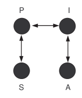
Figure 12: Bi-directed graph for Torus data

Table 5 reports the posterior means and standard deviations for the marginal log-linear interactions obtained via $10000$ iteration with a burn in of $1000$ with the proposed PAA algorithm and the RW-$\lambda$. The maximum likelihood estimates (MLEs) and corresponding approximate standard errors are also reported for comparative purposes. MLEs are obtained implementing an algorithm for the optimization of the Lagrangian log-likelihood which includes a set of zero constraints satisfying the marginal independence model; see Lupparelli (2006) for details. Standard errors for the parameter estimates can be simply derived from the estimate of the Hessian matrix of the Lagrangian log-likelihood; see Aitchison and Silvey (1958).

Table 5: Posterior summaries and MLEs for marginal log-linear interactions for the Torus Mandibularis data

	PAA		RW-$\lambda$		ML
	Mean	SD	Mean	SD	Estimate	SE
$\lambda^{AP}_{\emptyset}$	-1.391	0.004	-1.391	0.004
$\lambda^{AP}_{A}(2)$	-0.001	0.042	-0.003	0.043	-0.002	0.043
$\lambda^{AP}_{P}(2)$	-0.072	0.043	-0.079	0.043	-0.072	0.043
$\lambda^{AP}_{AP}(2,2)$	0.000	0.000	0.000	0.000	0.000
$\lambda^{AS}_{S}(2)$	-0.697	0.053	-0.695	0.055	-0.699	0.054
$\lambda^{AS}_{AS}(2,2)$	0.000	0.000	0.000	0.000	0.000
$\lambda^{IS}_{I}(2)$	0.234	0.045	0.241	0.044	0.232	0.044
$\lambda^{IS}_{IS}(2,2)$	0.000	0.000	0.000	0.000	0.000
$\lambda^{APS}_{PS}(2,2)$	0.004	0.053	-0.009	0.055	0.003	0.054
$\lambda^{APS}_{APS}(2,2,2)$	0.000	0.000	0.000	0.000	0.000
$\lambda^{AIS}_{AI}(2,2)$	-0.509	0.051	-0.505	0.052	-0.507	0.051
$\lambda^{AIS}_{AIS}(2,2,2)$	0.000	0.000	0.000	0.000	0.000
$\lambda^{AIPS}_{IP}(2,2)$	0.057	0.058	0.082	0.063	0.052	0.062
$\lambda^{AIPS}_{AIP}(2,2,2)$	0.132	0.068	0.049	0.065	0.151	0.062
$\lambda^{AIPS}_{ISP}(2,2,2)$	0.029	0.041	0.066	0.063	0.072	0.062
$\lambda^{AIPS}_{AIPS}(2,2,2)$	0.047	0.046	0.034	0.063	0.037	0.062

From Table 5 we observe that the posterior estimates (for both MCMC methods) and the MLEs coincide for all interactions and main effects obtained by marginals where no latent variable is involved; also Figure D.1 in the Appendix. This is not the case for $\lambda^{AIPS}_{IP}(2,2)$, $\lambda^{AIPS}_{IPS}(2,2,2)$, $\lambda^{AIPS}_{AIPS}(2,2,2)$, where the latent variable is involved. More specifically, the posterior standard deviations are lower by $6.5\%$, $34\%$ and $26\%$, respectively. This result is intuitively expected since PAA moves across the correct posterior distribution defined on the space of parameterisation with compatible marginal probabilities. On the other hand, both the RW-$\lambda$ and the approximate MLEs standard errors are obtained without considering the restrictions imposed in order to obtain parameterisations leading to compatible marginal probabilities.

Finally, differences are also observed for interaction $\lambda^{AIPS}_{AIP}(2,2,2)$ where RW-$\lambda$ provides posterior means far away from the corresponding MLEs with PAA being quite closely and standard deviance slightly higher than both the corresponding values of RW-$\lambda$ and the MLEs standard errors.

In terms of computational time, PAA was found to be faster with elapsed CPU time lower by $46\%$ compared with the corresponding one for RW-$\lambda$ (32.6 versus 60.8 seconds for 1000 iterations). Equivalently, the reported user CPU time was $48\%$ lower for PAA than the one for RW-$\lambda$ (29.9 versus 57.2 seconds for 1000 iterations). All runs were performed in a Windows 10 PC Intel Core i7-5500U CPU 2.4GHz with 16GB memory; all timings were obtained with the system.time function in R.

For 11,000 iterations, the effective sample size (ESS) of the methods are of similar size ranging from $43\%$ in favour of RW-$\lambda$ (for S main effect) to $36\%$ in favour of our method (for the four-way interaction).

Taking into consideration also the computational time of the two algorithms, the MCMC efficiency (ESS/Elapsed CPU time) for the proposed algorithm is considerably higher for all interactions ranging from $2\%$ increase to $141\%$. The average relative MCMC efficiency is higher for our method by $65\%$ compared with the one of the random walk MCMC. The above statistics were calculated with the effectiveSize function of coda package in R. The overall picture is similar if we consider results using the monitor function of rstan package in R; see Figure 13 for a visual representation of the relative efficiency for all interactions.

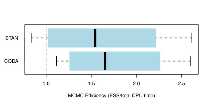
Figure 13: Boxplots of the relative efficiency of Prior-Adjustment Algorithm (PAA) compared to the random walk MCMC obtained by CODA and STAN for the Torus Mandibularis data

Finally, the MCMC errors were lower for the majority of the interactions by using the naive estimator of CODA package with relative values ranging from $0.61$ up to $1.13$ while the corresponding relative values for the time series based estimator are ranging from $0.66$ up to $1.30$. The naive estimator of MCE is simply given by the usual standard error ignoring autocorrelation (i.e. the MCMC estimated posterior standard deviation over the square root of the number of iterations).

6 Discussion

A possible way to parametrise discrete graphical models of marginal independence is by using the log-linear marginal models of Bergsma and Rudas (2002). The marginal log-linear interactions are calculated from specific marginals of the original table, and independencies imply zero constraints on specific set of interactions in a similar manner as in conditional log-linear graphical models.

In this work we focus on the Bayesian estimation of the log-linear interactions for graphical models of marginal independence. In particular, the method we propose allows us to assign prior directly on marginal log-linear interactions rather than on the probability interactions. This facilitates the incorporation of prior information since several models of interest can be specified by zero/linear constraints on log-linear terms. Bayesian analysis of such models is not widespread mainly due to the computational problems involved in the derivation of their posterior distribution. More specifically, MCMC methods need to be used since no conjugate analysis is available. Major difficulties arise from the fact that we need to sample from a posterior distribution defined on the space of parameterisations with compatible marginal probability distributions. In the proposed algorithms (PBIS and PAA), we satisfy such restrictions by sampling from the probability space of the graphical model of marginal independence under consideration. Then we transform the probability parameter values to the corresponding marginal log-linear ones avoiding the iterative procedure needed for the evaluation of the likelihood. In order to achieve this, we exploit the augmented DAG representation of the model. This not only facilitates the prior elicitation but also the construction of the Jacobian matrix involved in the acceptance probability of the induced Metropolis steps. PBIS is a more elaborate method but it leads to an automatic setup for sampling log-linear interactions by the posterior distribution. On the other hand, PAA can be implemented in a more straightforward manner. It leads to an efficient and fully automatic setup, which can be thought as a approximate method for sampling from the posterior distribution. It further avoids any time-consuming and troublesome tuning of MCMC parameters.

For future research, the authors would like to exploit and study the connections between the prior and the posterior distributions for the two different parameterisations (probability versus marginal log-linear). Moreover, extension of the method to accommodate fully automatic selection, comparison and model averaging techniques is an intriguing topic for further investigation.

Supplementary Material

Supplementary Material: Appendix for the Paper “Probability Based Independence Sampler for Bayesian Quantitative Learning in Graphical Log-Linear Marginal Models” (available at http://www.stat-athens.aueb.gr/~jbn/papers/files/2016_Ntzoufras_Tarantola_Lupparelli_Supplementary.pdf). The supplementary material includes details for the Jacobian calculations (Appendix A) and details for the construction of ${\mathbf{M}}$ and ${\mathbf{C}}$ matrices (Appendices B and C respectively). Finally, some additional results for the illustrated examples of Section 5 are provided in Appendix D.

Supplementary Material: Appendix for the Paper “Probability Based Independence Sampler for Bayesian Quantitative Learning in Graphical Log-Linear Marginal Models”

Ioannis Ntzoufras,	Claudia Tarantola	and	Monia Lupparelli
Athens University of Economics	University of Pavia, Italy		University of Bologna, Italy
& Business, Greece

Appendix A Jacobian calculations

Equation (13) can be rewritten as

$$\frac{\partial\lambda_{k}}{\partial\Pi_{\jmath}}=\sum\limits_{l=1}^{\textsc{c}_{C}}Q_{kl\jmath}\mbox{~{}~{}with~{}~{}}Q_{kl\jmath}=C_{kl}\frac{\sum\limits_{\imath=1}^{|{\cal I}|}M_{l\imath}\Delta_{\imath\jmath}}{\sum\limits_{\imath=1}^{|{\cal I}|}M_{l\imath}P_{\imath}},$$

where $\mbox{\boldmath$M$}=(M_{l\imath})$ is a $\textsc{c}_{C}\times|\cal{I}|$ matrix, $\mbox{\boldmath$\Delta$}=(\Delta_{\imath\jmath})$ is a matrix of dimension $|{\cal I}|\times d_{\Pi}$, and $d_{\Pi}$ is the dimension of the parameter vector $\Pi$.

A.1 Step-by-step computation of the Jacobian matrix

Once $\Delta$ is obtained (see Appendix A.2), we can construct the Jacobian matrix using the following steps

1. construct $\mbox{\boldmath$H$}=\mbox{\boldmath$M$}\mbox{\boldmath$\Delta$}$ a matrix of dimension $\textsc{c}_{C}\times dim(\Pi)$;

2. construct $\mbox{\boldmath$\Gamma$}=\mbox{\boldmath$M$}\mbox{\boldmath$P$}$ vector of dimension $\textsc{c}_{C}\times 1$;

3. construct $\mbox{\boldmath$\Gamma$}^{\prime}=\mbox{\boldmath$\Gamma$}\mbox{\boldmath$1$}_{d_{\Pi}}^{T}$, with $\mbox{\boldmath$1$}_{d}$ a $d_{\Pi}\times 1$ vector of ones, and $\mbox{\boldmath$\Gamma$}^{\prime}$ a matrix of dimension $\textsc{c}_{C}\times d_{\Pi}$ with all columns equal to $\Gamma$;

4. set $\mbox{\boldmath$H$}^{\prime}=\mbox{\boldmath$H$}\circ\mbox{\boldmath$\Gamma$}^{\prime\prime}$ where $\circ$ indicates the Hadamard product (element by element multiplication), and $\mbox{\boldmath$\Gamma$}^{\prime\prime}$ is a matrix with elements $\Gamma^{\prime\prime}_{\nu\kappa}=1/\Gamma^{\prime}_{\nu\kappa}$;

5. denote with $\mbox{\boldmath$J$}=\mbox{\boldmath$C$}\mbox{\boldmath$H$}^{\prime}$ the Jacobian matrix dimension $d_{\Pi}\times d_{\Pi}$.

A.2 Computational details for the elements of $\Delta$

We now describe how we can analytically obtain the elements of matrix $\Delta$ defined in (14). Each element of this matrix is derivative of type $\dfrac{\partial p(i)}{\partial\pi_{u|pa(u)}\big{(}j_{u}|j_{pa(u)}\big{)}}$, $i\in{\cal I}$ and $j\in{\cal I}^{\cal A}$. We can separate the computations in two separate cases:

Case A:

$u\in{\cal V}$, i.e. $u$ is an observable variable.

Case B:

$u\in{\cal L}$, i.e. $u$ is a latent variable.

A.2.1 Case A: Computations for Expression (15)

For any variable $u\in{\cal V}$ and $j_{u}<|{\cal I}_{u}|$ we have that

$$\dfrac{\partial p(i)}{\partial\pi_{u|pa(u)}\big{(}j_{u}|j_{pa(u)}\big{)}}=\dfrac{\partial\sum\limits_{i_{\cal L}\in{\cal I}_{\cal L}}p^{\cal A}\big{(}i,i_{\cal L}\big{)}}{\partial\pi_{u|pa(u)}\big{(}j_{u}|j_{pa(u)}\big{)}}=\sum_{i^{*}_{\cal L}\in{\cal I}_{{\cal L}}}\dfrac{\partial p^{\cal A}\big{(}i^{*}\big{)}}{\partial\pi_{u|pa(u)}\big{(}j_{u}|j_{pa(u)}\big{)}}$$

since $i^{*}=(i,i_{\cal L})\Leftrightarrow i^{*}_{\cal V}=i$ and $i^{*}_{\cal L}=i_{\cal L}$. From (7) we further obtain that

$$\dfrac{\partial p(i)}{\partial\pi_{u|pa(u)}\big{(}j_{u}|j_{pa(u)}\big{)}}=$$ (18)

$$= \sum_{i^{*}_{\cal L}\in{\cal I}_{{\cal L}}}\frac{\partial\left\{\pi_{u|pa(u)}\big{(}i^{*}_{u}|i^{*}_{pa(u)}\big{)}\prod\limits_{v\in{\cal V}\cup{\cal L}\setminus u}\ \pi_{v|pa(v)}\big{(}i^{*}_{v}|i^{*}_{pa(v)}\big{)}\right\}}{\partial\pi_{u|pa(u)}\big{(}j_{u}|j_{pa(u)}\big{)}}=$$

$$= \sum_{i^{*}_{\cal L}\in{\cal I}_{{\cal L}}}\left\{\left[\prod\limits_{v\in{\cal V}\cup{\cal L}\setminus u}\ \pi_{v|pa(v)}\big{(}i^{*}_{v}|i^{*}_{pa(v)}\big{)}\right]\times\frac{\partial\pi_{u|pa(u)}\big{(}i^{*}_{u}|i^{*}_{pa(u)}\big{)}}{\partial\pi_{j_{u}|pa(u)}\big{(}j_{u}|j_{pa(u)}\big{)}}\right\}=$$

$$= \sum_{i^{*}_{\cal L}\in{\cal I}_{{\cal L}}}\left\{\left[\prod\limits_{v\in{\cal V}\cup{\cal L}\setminus u}\ \pi_{v|pa(v)}\big{(}i^{*}_{v}|i^{*}_{pa(v)\setminus{\cal L}},i^{*}_{{\cal L}_{v}}\big{)}\right]\times\frac{\partial\pi_{u|pa(u)}\big{(}i^{*}_{u}|i^{*}_{pa(u)\setminus{\cal L}},i^{*}_{{\cal L}_{u}}\big{)}}{\partial\pi_{u|pa(u)}\big{(}j_{u}|j_{pa(u)\setminus{\cal L}},j_{{\cal L}_{u}}\big{)}}\right\},$$

where ${\cal L}_{u}={\cal L}\cap pa(u)$, is the set latent variables ${\cal L}$ that are parents of $u$. In the following we indicate with by $\overline{{\cal L}_{u}}={\cal L}\setminus pa(u)$ the latent variables that are not parents of $u$.

Therefore, (18) can be rewritten

$$\dfrac{\partial p(i)}{\partial\pi_{u|pa(u)}(j_{u}|j_{pa(u)})}=$$

$$= \sum_{i^{*}_{\overline{{\cal L}_{u}}}\in{\cal I}_{\overline{{\cal L}_{u}}}}\left\{\sum_{i^{*}_{{\cal L}_{u}}\in{\cal I}_{{\cal L}_{u}}}\left[\prod\limits_{v\in{\cal V}\cup({\cal L}_{u}\cup\overline{{\cal L}_{u}})\setminus u}\ \pi_{v|pa(v)}\big{(}i^{*}_{v}|i^{*}_{pa(v)\setminus{\cal L}},i^{*}_{{\cal L}_{v}}\big{)}\times\frac{\partial\pi_{u|pa(u)}\big{(}i^{*}_{u}|i^{*}_{pa(u)\setminus{\cal L}},i^{*}_{{\cal L}_{u}}\big{)}}{\partial\pi_{u|pa(u)}\big{(}j_{u}|j_{pa(u)\setminus{\cal L}},j_{{\cal L}_{u}}\big{)}}\right]\right\}$$

$$= \sum_{i^{*}_{\overline{{\cal L}_{u}}}\in{\cal I}_{\overline{{\cal L}_{u}}}}\left\{\sum_{i^{*}_{{\cal L}_{u}}\in{\cal I}_{{\cal L}_{u}}}\left[\prod\limits_{v\in\overline{{\cal L}_{u}}}\ \pi_{v|pa(v)}\big{(}i^{*}_{v}|i^{*}_{pa(v)\setminus{\cal L}},i^{*}_{{\cal L}_{v}}\big{)}\right.\right.$$

$$\hskip 71.13188pt\left.\left.\times\prod\limits_{v\in{\cal V}\cup{\cal L}_{u}\setminus u}\ \pi_{v|pa(v)}\big{(}i^{*}_{v}|i^{*}_{pa(v)\setminus{\cal L}},i^{*}_{{\cal L}_{v}}\big{)}\times\frac{\partial\pi_{u|pa(u)}\big{(}i^{*}_{u}|i^{*}_{pa(u)\setminus{\cal L}},i^{*}_{{\cal L}_{u}}\big{)}}{\partial\pi_{u|pa(u)}\big{(}j_{u}|j_{pa(u)\setminus{\cal L}},j_{{\cal L}_{u}}\big{)}}\right]\right\}$$

$$= \sum_{i^{*}_{\overline{{\cal L}_{u}}}\in{\cal I}_{\overline{{\cal L}_{u}}}}\left\{\left[\prod\limits_{v\in\overline{{\cal L}_{u}}}\ \pi_{v|pa(v)}\big{(}i^{*}_{v}|i^{*}_{pa(v)\setminus{\cal L}},i^{*}_{{\cal L}_{v}}\big{)}\right]\right.$$

$$\left.\times\sum_{i^{*}_{{\cal L}_{u}}\in{\cal I}_{{\cal L}_{u}}}\left(\prod\limits_{v\in{\cal V}\cup{\cal L}_{u}\setminus u}\ \pi_{v|pa(v)}\big{(}i^{*}_{v}|i^{*}_{pa(v)\setminus{\cal L}},i^{*}_{{\cal L}_{v}}\big{)}\times\frac{\partial\pi_{u|pa(u)}\big{(}i^{*}_{u}|i_{pa(u)\setminus{\cal L}},i^{*}_{{\cal L}_{u}}\big{)}}{\partial\pi_{u|pa(u)}\big{(}j_{u}|j_{pa(u)\setminus{\cal L}},j_{{\cal L}_{u}}\big{)}}\right)\right\}.(19)$$

We now concentrate on the second line of (A.2.1), that is

$$\sum_{i^{*}_{{\cal L}_{u}}\in{\cal I}_{{\cal L}_{u}}}\left(\prod\limits_{v\in{\cal V}\cup{\cal L}_{u}\setminus u}\ \pi_{v|pa(v)}\big{(}i^{*}_{v}|i^{*}_{pa(v)\setminus{\cal L}},i^{*}_{{\cal L}_{v}}\big{)}\times\frac{\partial\pi_{u|pa(u)}\big{(}i^{*}_{u}|i^{*}_{{\cal L}_{u}},i^{*}_{pa(u)\setminus{\cal L}}\big{)}}{\partial\pi_{u|pa(u)}\big{(}j_{u}|j_{{\cal L}_{u}},j_{pa(u)\setminus{\cal L}}\big{)}}\right)=$$

$$\hskip 28.45274pt=\begin{cases}~{}~{}~{}\prod\limits_{v\in{\cal V}\cup{\cal L}_{u}\setminus u}\ \pi_{v|pa(v)}\big{(}i^{*}_{v}|i^{*}_{pa(v)}\big{)}&\mbox{~{}if~{}}i^{*}_{u}=j_{u}<|{\cal I}_{u}|\mbox{~{}and~{} }i^{*}_{pa(u)}=j_{pa(u)}\\ -\prod\limits_{v\in{\cal V}\cup{\cal L}_{u}\setminus u}\ \pi_{v|pa(v)}\big{(}i^{*}_{v}|i^{*}_{pa(v)}\big{)}&\mbox{~{}if~{}}j_{u}\neq i^{*}_{u}=|{\cal I}_{u}|\mbox{~{}and~{} }i^{*}_{pa(u)}=j_{pa(u)}\\ ~{}~{}~{}~{}~{}~{}~{}~{}0&\mbox{~{}if~{}}j_{u}\neq i^{*}_{u}<|{\cal I}_{u}|\mbox{~{}or~{} }i^{*}_{pa(u)}\neq j_{pa(u)}\\ \end{cases}\,.$$

In the case where $i^{*}_{u}=j_{u}<|{\cal I}_{u}|$ and $i_{pa(u)\setminus{\cal L}}=j_{pa(u)\setminus{\cal L}}$ then

$$\dfrac{\partial p(i)}{\partial\pi_{u|pa(u)}\big{(}j_{u}|j_{pa(u)}\big{)}}=$$

$$= \sum_{i^{*}_{\overline{{\cal L}_{u}}}\in{\cal I}_{\overline{{\cal L}_{u}}}}\left\{\left[\prod\limits_{v\in\overline{{\cal L}_{u}}}\ \pi_{v|pa(v)}\big{(}i^{*}_{v}|i^{*}_{pa(v)}\big{)}\right]\prod\limits_{v\in{\cal V}\cup{\cal L}_{u}\setminus u}\ \pi_{v|pa(v)}\big{(}i^{*}_{v}|i^{*}_{pa(v)}\big{)}I_{\{i^{*}_{pa(u)}=j_{pa(u)}\}}\right\}$$

$$= \sum_{i^{*}_{\overline{{\cal L}_{u}}}\in{\cal I}_{\overline{{\cal L}_{u}}}}\left\{\prod\limits_{v\in{\cal V}\cup{\cal L}\setminus u}\ \pi_{v|pa(v)}\big{(}i^{*}_{v}|i^{*}_{pa(v)}\big{)}I_{\{i^{*}_{pa(u)}=j_{pa(u)}\}}\right\}$$

$$= \sum_{i^{*}_{\overline{{\cal L}_{u}}}\in{\cal I}_{\overline{{\cal L}_{u}}}}\left\{\dfrac{\pi_{u|pa(u)}(i^{*}_{u}|i^{*}_{pa(u)})}{\pi_{u|pa(u)}(i^{*}_{u}|i^{*}_{pa(u)})}\prod\limits_{v\in{\cal V}\cup{\cal L}\setminus u}\ \pi_{v|pa(v)}\big{(}i^{*}_{v}|i^{*}_{pa(v)}\big{)}I_{\{i^{*}_{pa(u)}=j_{pa(u)}\}}\right\}$$

$$= \sum_{i^{*}_{\overline{{\cal L}_{u}}}\in{\cal I}_{\overline{{\cal L}_{u}}}}\left\{\dfrac{p^{\cal A}(i,j_{{\cal L}_{u}},j_{\overline{{\cal L}_{u}}})}{\pi_{u|pa(u)}(i^{*}_{u}|j_{pa(u)})}\right\}=\frac{\sum\limits_{i^{*}_{\overline{{\cal L}_{u}}}\in{\cal I}_{\overline{{\cal L}_{u}}}}p^{\cal A}(i,j_{{\cal L}_{u}},j_{\overline{{\cal L}_{u}}})}{\pi_{u|pa(u)}(i^{*}_{u}|j_{pa(u)})}\,.$$

Finally we obtain that

$$\dfrac{\partial p(i)}{\partial\pi_{u|pa(u)}\big{(}j_{u}|j_{pa(u)}\big{)}}=\frac{p^{{\cal A}_{u}}(i,j_{{\cal L}_{u}})}{\pi_{u|pa(u)}(i^{*}_{u}|j_{pa(u)})}\,.$$ (20)

In a similar way, we find that

$$\dfrac{\partial p(i)}{\partial\pi_{u|pa(u)}(j_{u}|j_{pa(u)})}=-\frac{p^{{\cal A}_{u}}(i,j_{{\cal L}_{u}})}{\pi_{u|pa(u)}(i^{*}_{u}|j_{pa(u)})}$$ (21)

for $j_{u}\neq i^{*}_{u}=|{\cal I}_{u}|$ and $i_{pa(u)\setminus{\cal L}}=j_{pa(u)\setminus{\cal L}}$.

Finally, if $j_{u}\neq i^{*}_{u}<|{\cal I}_{u}|\mbox{~{}or~{} }i_{pa(u)\setminus{\cal L}}\neq j_{pa(u)\setminus{\cal L}}$, (A.2.1) will become equal to

$$\dfrac{\partial p(i)}{\partial\pi_{u|pa(u)}(i^{*}_{u}|j_{pa(u)})}=0.$$ (22)

Since $u$ is an observed variable $i_{u}\equiv i^{*}_{u}$, from equations (20)–(22), we obtain the final expressions

$$\dfrac{\partial p(i)}{\partial\pi_{u|pa(u)}\big{(}j_{u}|j_{pa(u)}\big{)}}=\delta(i,j)\frac{p^{{\cal A}_{u}}\big{(}i,j_{{\cal L}_{u}})}{\pi_{u|pa(u)}(i_{u}|j_{pa(u)}\big{)}}$$

with

$$\delta(i,j)=\begin{cases}~{}~{}~{}1&\mbox{~{}if~{}}i_{u}=j_{u}<|{\cal I}_{u}|$ and $i_{pa(u)\setminus{\cal L}}=j_{pa(u)\setminus{\cal L}}\vspace{0.5em}\\ -1&\mbox{~{}if~{}}j_{u}\neq i_{u}=|{\cal I}_{u}|$ and $i_{pa(u)\setminus{\cal L}}=j_{pa(u)\setminus{\cal L}}\\ ~{}~{}~{}0&\mbox{~{}if~{}}j_{u}\neq i_{u}<|{\cal I}_{u}|$ or $\;\;i_{pa(u)\setminus L}\neq j_{pa(u)\setminus{\cal L}}\end{cases}~{},$$

where

$$p^{{\cal A}_{u}}\big{(}i,j_{{\cal L}_{u}}\big{)}=\begin{cases}P\Big{(}Y_{\cal V}=i,Y_{{\cal L}\cap pa(u)}=j_{{\cal L}\cap pa(u)}\Big{)}&{\cal L}_{u}\neq\emptyset\\ p(i)&{\cal L}_{u}=\emptyset\end{cases}.$$

A.2.2 Case B: Computations for Expression (17)

For every latent variable $u\in{\cal L}$ the parent set is empty. Hence $\pi_{u|pa(u)}\big{(}i^{*}_{u}|i^{*}_{pa(u)}\big{)}=\pi_{u}\big{(}i^{*}_{u}\big{)}$ for all $i^{*}\in{\cal A}$. Furthermore, it holds that $p(i)=\sum\limits_{i_{\cal L}\in{\cal I}_{\cal L}}p^{\cal A}(i,i_{\cal L})=\sum\limits_{i^{*}_{\cal L}\in{\cal I}_{\cal L}}p^{\cal A}(i^{*})$ .

Therefore, for any parameter $\pi_{u}(j_{u})$ with $j_{u}\neq|{\cal I}_{u}|$ and $u\in{\cal L}$, the derivative is given by

$$\frac{\partial p(i)}{\partial\pi_{u}(j_{u})} = \frac{\partial\sum\limits_{i_{\cal L}\in{\cal I}_{\cal L}}p^{\cal A}(i,i_{\cal L})}{\partial\pi_{u}(j_{u})}=\frac{\partial\sum\limits_{i^{*}_{\cal L}\in{\cal I}_{\cal L}}p^{\cal A}(i^{*})}{\partial\pi_{u}(j_{u})}=\sum\limits_{i^{*}_{\cal L}\in{\cal I}_{\cal L}}\frac{\partial p^{\cal A}(i^{*})}{\partial\pi_{u}(j_{u})}$$

$$= \sum_{i^{*}_{{\cal L}\setminus u}\in{\cal I}_{{\cal L}\setminus u}}\left\{\sum_{i^{*}_{u}\in{\cal I}_{u}}\dfrac{\partial\left\{\pi_{u}(i^{*}_{u})\prod\limits_{v\in{\cal V}\cup{\cal L}\setminus\{u\}}\ \pi_{v|pa(v)}\left(i^{*}_{v}|i^{*}_{pa(v)}\right)\right\}}{\partial\pi_{u}(j_{u})}\right\}$$

$$= \sum_{i^{*}_{{\cal L}\setminus u}\in{\cal I}_{{\cal L}\setminus u}}\left\{\sum_{i^{*}_{u}\in{\cal I}_{u}}\left[\dfrac{\partial\pi_{u}(i^{*}_{u})}{\partial\pi_{u}(j_{u})}\times\prod\limits_{v\in{\cal V}\cup{\cal L}\setminus\{u\}}\ \pi_{v|pa(v)}\left(i^{*}_{v}|i^{*}_{pa(v)}\right)\right]\right\}.$$

The derivatives involved in the above equation are given by

$$\dfrac{\partial\pi_{u}(i^{*}_{u})}{\partial\pi_{u}(j_{u})}=\begin{cases}~{}~{}~{}1&\mbox{if }j_{u}=i^{*}_{u}<|{\cal I}_{u}|\\ -1&\mbox{if }j_{u}\neq i^{*}_{u}=|{\cal I}_{u}|\\ ~{}~{}~{}0&\mbox{if }j_{u}\neq i^{*}_{u}<|{\cal I}_{u}|\end{cases}~{}.$$

Hence, we obtain

$$\frac{\partial p(i)}{\partial\pi_{u}(j_{u})} = \sum_{i^{*}_{{\cal L}\setminus u}\in{\cal I}_{{\cal L}\setminus u}}\bigg{\{}\prod\limits_{v\in{\cal V}\cup{\cal L}\setminus\{u\}}\ \pi_{v|pa(v)}(i^{*}_{v}|i^{*}_{pa(v)})I_{\{i^{*}_{u}=j_{u}\}}$$

$$\hskip 37.00002pt-\prod\limits_{v\in{\cal V}\cup{\cal L}\setminus\{u\}}\ \pi_{v|pa(v)}(i^{*}_{v}|i^{*}_{pa(v)})I_{\{i^{*}_{u}=|{\cal I}_{u}|\}}\bigg{\}}$$

$$= \sum_{i^{*}_{{\cal L}\setminus u}\in{\cal I}_{{\cal L}\setminus u}}\bigg{\{}\dfrac{\pi_{u}(i^{*}_{u})}{\pi_{u}(i^{*}_{u})}\prod\limits_{v\in{\cal V}\cup{\cal L}\setminus\{u\}}\ \pi_{v|pa(v)}(i^{*}_{v}|i^{*}_{pa(v)})I_{\{i^{*}_{u}=j_{u}\}}$$

$$\hskip 37.00002pt-\dfrac{\pi_{u}(i^{*}_{u})}{\pi_{u}(i^{*}_{u})}\prod\limits_{v\in{\cal V}\cup{\cal L}\setminus\{u\}}\ \pi_{v|pa(v)}(i^{*}_{v}|i^{*}_{pa(v)})I_{\{i^{*}_{u}=|{\cal I}_{u}|\}}\bigg{\}}$$

$$= \sum_{i^{*}_{{\cal L}\setminus u}\in{\cal I}_{{\cal L}\setminus u}}\bigg{\{}\dfrac{p^{\cal A}(i^{*}_{\cal V},j_{u},i^{*}_{{\cal L}\setminus u})}{\pi_{u}(j_{u})}-\dfrac{p^{\cal A}(i^{*}_{\cal V},|{\cal I}_{u}|,i^{*}_{{\cal L}\setminus u})}{\pi_{u}(|{\cal I}_{u}|)}\bigg{\}}$$

$$= \dfrac{p^{{\cal A}_{u}}(i^{*}_{\cal V},j_{u})}{\pi_{u}(j_{u})}-\dfrac{p^{{\cal A}_{u}}(i^{*}_{\cal V},|{\cal I}_{u}|)}{\pi_{u}(|{\cal I}_{u}|)}$$

$$= \dfrac{p^{{\cal A}_{u}}(i,j_{u})}{\pi_{u}(j_{u})}-\dfrac{p^{{\cal A}_{u}}(i,|{\cal I}_{u}|)}{\pi_{u}(|{\cal I}_{u}|)},$$

where $i=i^{*}_{\cal V}$ and this concludes the computation of (17).

Appendix B Construction of Matrix $\mathbf{M}$

Let ${\cal M}=\Big{\{}M_{1},M_{2},\dots,M_{|{\cal M}|}\Big{\}}$ be the set of marginals under consideration by a given marginal log-linear parameterisation. Let ${\mathbf{B}}$ be a binary matrix of dimension $|\cal M|\times|{\cal V}|$ with elements $B_{mv}$ indicating whether a variable $v$ belongs to a specific marginal $M_{m}$. The rows of ${\mathbf{B}}$ correspond to the marginals in ${\cal M}$ whereas the columns to the variables. The variables follow a reverse ordering, that is column 1 corresponds to variable $Y_{|\cal V|}$, column 2 to variable $Y_{|{\cal V}|-1}$ and so on. Matrix $\mathbf{B}$ has elements

$$B_{mv}=\left\{\begin{array}[]{rl}1&\mbox{ if $v\in M_{m}$ }\\ 0&\mbox{ otherwise.}\end{array}\right.$$

for every $v\in\cal V$.

The marginalisation matrix $\mathbf{M}$ can be obtained applying the following rules.

1. For each marginal $M_{m}$ and each variable $v$ we construct the following matrix

   $${\mathbf{A}}_{m,v}=\left\{\begin{array}[]{rl}{\mathbf{I}}_{|{\cal I}_{v}|}&\mbox{ if }\;\;B_{mv}=1\\ {\mathbf{1}}_{|{\cal I}_{v}|}^{T}&\mbox{ if }\;\;B_{mv}=0\end{array},\right.$$

   where ${\mathbf{I}}_{|{\cal I}_{v}|}$ is the identity matrix of dimension $|{\cal I}_{v}|\times|{\cal I}_{v}|$ and ${\mathbf{1}}_{|{\cal I}_{v}|}$ is a vector of dimension $|{\cal I}_{v}|\times 1$ with all elements equal to one.

   The probability vector of the marginal table corresponding to $M_{m}$ is given by $\mathbf{M}_{m}\mathbf{\pi}$; where $\mathbf{M}_{m}$ is calculated as a Kronecker product of matrices ${\mathbf{A}}_{mv}$

   $$\mathbf{M}_{m} = \bigotimes_{q=0}^{|{\cal V}|-1}{\mathbf{A}}_{m,|{\cal V}|-q}$$

   $$= {\mathbf{A}}_{m,|{\cal V}|}\bigotimes{\mathbf{A}}_{m,|{\cal V}|-1}\bigotimes\dots\bigotimes{\mathbf{A}}_{m,2}\bigotimes{\mathbf{A}}_{m,1},$$

   where $\bigotimes$ denotes the Kronecker product which is implemented in reverse lexicographical order (starting from the last on in ${\cal V}$).

2. Matrix $\mathbf{M}$ is constructed by stacking all the $\mathbf{M}_{m}$ matrices

   $$\mathbf{M}=\left(\begin{array}[]{l}\mathbf{M}_{1}\\ \vdots\\ \mathbf{M}_{m}\\ \vdots\\ \mathbf{M}_{|{\cal M}|}\end{array}\right)~{}.$$

Appendix C Construction of Matrix $\mathbf{C}$

Firstly we need to construct the design matrix ${\mathbf{X}}_{\cal V}$ for the saturated model for the cross-classification of discrete variables $Y_{\cal V}$ with sum to zero constraints. Firstly, for each variable $v$ we construct the following matrix

$${\mathbf{J}}_{v}=\left(\begin{array}[]{ll}1&-\mathbf{1}^{T}_{(|{\cal I}_{v}|-1)}\\ \mathbf{1}_{(|{\cal I}_{v}|-1)}&~{}~{}~{}\mathbf{I}_{(|{\cal I}_{v}|-1)}\end{array}\right)~{},$$

where ${\mathbf{1}}_{\kappa}$ is a vector of ones of length $\kappa$ while $\mathbf{I}_{\kappa}$ is the identity matrix of dimension $\kappa\times\kappa$.

The design matrix of the satured model will be of dimension $\left(\prod\limits_{v\in{\cal V}}|{\cal I}_{v}|\right)\times\left(\prod\limits_{v\in{\cal V}}|{\cal I}_{v}|\right)$ and can be obtained as

$$\mathbf{Y}_{\cal V}=\bigotimes_{q=0}^{|{\cal V}|-1}{\mathbf{J}}_{|{\cal V}|-q}~{}.$$

The contrast matrix $\mathbf{C}$ can be constructed by using the following rules.

1. For each margin $M_{m}$, we construct the design matrix ${\mathbf{X}}_{M_{m}}$ corresponding to the saturated model (using sum-to-zero constraints) of the cross-classification of variables $Y_{M_{m}}$. Then we consider its inverse ${\mathbf{X}}_{M_{m}}^{-1}$ in order to obtain the corresponding contrast matrix. Now, let $\mathbf{C}_{m}$ be a sub-matrix of the contrast matrix ${\mathbf{X}}_{M_{m}}^{-1}$ obtained by deleting rows corresponding to interactions that are not obtained from margin $M_{m}$.

2. The contrast matrix $\mathbf{C}$ is obtained as

   $$\mathbf{C}=\bigoplus_{m:~{}M_{m}\in{\cal M}}\mathbf{C}_{m}=\mbox{diag}(C_{1},\ldots,C_{|\cal M|})~{},$$

   where $\bigoplus$ denotes the matrix direct sum.

Appendix D Additional Results

Figure D.1 depicts the posterior ergodic plots for the estimates of the elements of $\vec{\mbox{\boldmath$\lambda$}}$ obtained using PAA and the corresponding approximate MLE based statistics for the real dataset of Section 5.2.

Figure D.1: Ergodic plots for marginal log-linear interactions using Prior-Adjustment Algorithm (PAA) compared with approximate maximum likelihood estimates for the Torus Mandibularis data

\psfrag{A2}[c][b][0.7]{$\lambda_{\scriptscriptstyle A}^{\scriptscriptstyle AP}$}\psfrag{C2}[c][b][0.7]{$\lambda_{\scriptscriptstyle P}^{\scriptscriptstyle AP}$}\psfrag{B2}[c][b][0.7]{$\lambda_{\scriptscriptstyle I}^{\scriptscriptstyle IS}$}\psfrag{D2}[c][b][0.7]{$\lambda_{\scriptscriptstyle S}^{\scriptscriptstyle AS}$}\psfrag{C2D2}[c][b][0.7]{$\lambda_{\scriptscriptstyle PS}^{\scriptscriptstyle APS}$}\psfrag{A2B2}[c][b][0.7]{$\lambda_{\scriptscriptstyle AI}^{\scriptscriptstyle AIS}$}\psfrag{B2C2}[c][b][0.7]{$\lambda_{\scriptscriptstyle IS}^{\scriptscriptstyle IS}$~{}}\psfrag{A2D2}[c][b][0.7]{$\lambda_{\scriptscriptstyle AS}^{\scriptscriptstyle AS}$}\psfrag{A2B2C2}[c][b][0.7]{$\lambda_{\scriptscriptstyle AIP}^{\scriptscriptstyle AIPS}$}\psfrag{A2B2D2}[c][b][0.7]{$\lambda_{\scriptscriptstyle AIS}^{\scriptscriptstyle AIS}$}\psfrag{A2C2D2}[c][b][0.7]{$\lambda_{\scriptscriptstyle APS}^{\scriptscriptstyle APS}$}\psfrag{B2C2D2}[c][b][0.7]{~{}~{}$\lambda_{\scriptscriptstyle IPS}^{\scriptscriptstyle AIPS}$}\psfrag{B2D2}[c][b][0.7]{~{}~{}$\lambda_{\scriptscriptstyle IS}^{\scriptscriptstyle IS}$}\psfrag{A2B2C2D2}[c][b][0.7]{~{}~{}~{}~{}~{}~{}~{}~{}$\lambda_{\scriptscriptstyle AISP}^{\scriptscriptstyle AISP}$}\includegraphics[width=369.88582pt]{ergodic_plots.ps}

References

• Aitchison and Silvey (1958) Aitchison, J. and Silvey, S. D. (1958). Maximum likelihood estimation of parameters subject to restraints. Annals of Mathematical Statistics 29, 813–828.
• Bartolucci et al. (2012) Bartolucci, F., Scaccia, L. and Farcomeni, A. (2012). Bayesian inference through encompassing priors and importance sampling for a class of marginal models for categorical data. Computational Statistics and Data Analysis, 56, 4067–4080.
• Bergsma and Rudas (2002) Bergsma, W. P. and Rudas, T. (2002). Marginal log-linear models for categorical data. Annals of Statistics, 30, 140-159.
• Bergsma et al. (2009) Bergsma, W. O., Croon, M. A. and Hagenaars, J. A. (2009). Marginal Models. For Dependent, Clustered, and Longitudinal Categorical Data, Springer
• Bishop et al. (1975) Bishop, Y. M. M., Fienberg, S. E. and Holland, P. W. (1975). Multivariate Analysis, Theory and Practice, MIT press.
• Cox and Wermuth (1993) Cox, D. R. and Wermuth, N. (1993). Linear dependencies represented by chain graphs (with discussion). Statistical Science, 8, 204-218, 247-277.
• Dellaportas and Forster (1999) Dellaportas, P. and Forster, J.J.(1999). Markov Chain Monte Carlo model determination for hierarchical and graphical log-linear models. Biometrika, 86, 615-633.
• Drton and Richardson (2008) Drton, M. and Richardson, T. S. (2008). Binary models for marginal independence. Journal of the Royal Statistical Society, Ser. B , 70, 287-309.
• Evans (2016) Evans, R. J. (2016) Graphs for margins of Bayesian networks. Scandinavian Journal of Statistics, 43, 625-648.
• Evans and Richardson (2013) Evans, R. J. and Richardson, T. S. (2013) Marginal log-linear parameters for graphical Markov models. Journal of the Royal Statistical Society, Ser. B , 75, 743-768.
• Forcina et al. (2010) Forcina, A., Lupparelli, M., and Marchetti, G. M. (2010). Marginal parameterizations of discrete models defined by a set of conditional independencies. Journal of Multivariate Analysis, 101, 2519 - 2527.
• Knuiman and Speed (1988) Knuiman, M. W. and Speed, T. P. (1988). Incorporating prior information into the analysis of contingency tables. Biometrics, 44, 1061-1071.
• Lupparelli (2006) Lupparelli, M. (2006). Graphical models of marginal independence for categorical variables. Ph. D. thesis, University of Florence.
• Lupparelli et al. (2009) Lupparelli, M., Marchetti, G. M., Bersgma, W. P. (2009). Parameterization and fitting of bi-directed graph models to categorical data. Scandinavian journal of Statistics 36, 559-576.
• Muller and Mayhall (1971) Muller, T.P. and Mayhall, J.T. (1971). Analysis of contingency table data on torus mandibularis using a loglinear model. American Journal of Physical Anthropology, 34, 149-154.