Abstract

We report calculations of collision strengths and effective collision strengths for 26 allowed transitions among the $n\leq$ 5 degenerate levels of atomic hydrogen for which the close-coupling (CC) and Born approximations have been used. Results are listed over a wide range of energies (up to 50 Ryd) and temperatures (up to 10⁷ K), sufficient for applications over a variety of plasmas, including fusion. Similar results have also been calculated for deuterium, but they negligibly differ with those of hydrogen.

1 Introduction

Hydrogen is the most abundant element in the universe and therefore, atomic data for its emission lines are very important for various studies of astrophysical plasmas. This element is equally important for fusion, because it is the main fuel for burning in a reactor, and therefore the importance of its data has further increased with the developing ITER project. Energies for its levels and radiative rates (A-values) for its transitions are fairly well known – see for example, the compilations by Kramida [1] and Wiese and Fuhr [2], and the NIST (National Institute of Standards and Technology) website at http://www.nist.gov/pml/data/asd.cfm. However, the corresponding information about the collisional data for electron impact excitation lacks completeness. Most of the data, experimental or theoretical, are limited in the range of energy or the number of transitions, as summarised by Anderson et al.  [3] and Benda and Houfek [4], and further discussed below.

The first major study of collisional data for H was performed by us (Aggarwal et al. [5]), which included states with $n\leq$ 5. The calculations were based on the close-coupling $R$-matrix method and reported results for both collision strengths ($\Omega$) and effective collision strengths ($\Upsilon$), obtained after integrating the $\Omega$ data over a Maxwellian distribution of electron velocities – see a review by Henry [6] for the general background about electron atom/ion collisions. A notable deficiency of this work was that higher ionisation channels, at energies above thresholds, were not considered, and this leads to the overestimation of results, for some transitions. Therefore, Anderson et al. [3] included pseudostates in the expansion of wavefunctions in the $R$-matrix framework, and this allowed for the loss of electron flux into the continuum. They did not specifically list the $\Omega$ data but reported results for $\Upsilon$ for most (not all) transitions among the $n\leq$ 5 states of H. Unfortunately, questions were soon raised about the accuracy of their work, particularly at higher temperatures. Therefore, they subsequently corrected their results in a later paper [7]. Nevertheless, doubts remain about the accuracy and reliability of their data, as discussed by Lavrov and Pipa [8] and Wünderlich et al.  [9].

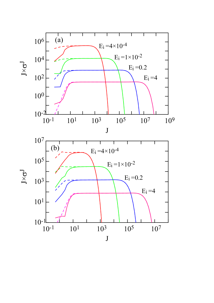
Figure 2: Variation of $J\times\sigma_{J}$ with partial waves $J$ for (a) 2p_1/2–2s_1/2 and (b) 2s_1/2–2p_3/2 transitions. Broken curves: Born and continuous curves: CC+Born results.

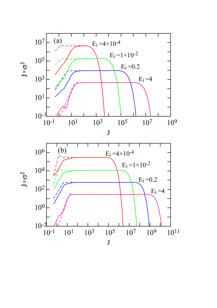
Figure 3: Variation of $J\times\sigma_{J}$ with partial waves $J$ for (a) 3s_1/2–3p_3/2 and (b) 3d_3/2–3p_3/2 transitions. Broken curves: Born and continuous curves: CC+Born results.

Recently, Benda and Houfek [4] have performed yet another calculation by employing a different approach, based on direct solution of the Schrödinger equation in the B-spline basis. They also made some improvements over the earlier results and concluded an overall good agreement with the $\Omega$ data of Aggarwal et al.  [5], although differences for a few transitions, particularly those from the ground 1s to higher excited states, are up to 12%. Although they presented their results for $\Omega$ only graphically, corresponding numerical data can be easily obtained, in a very fine energy mesh, from their website http://utf.mff.cuni.cz/data/hex. However, they did not report the corresponding data for $\Upsilon$, which are required for the modelling or diagnostics of the plasmas, and neither can these be calculated from their numerical data (except at very low temperatures), because of the limited energy range, below 1 Ryd. Therefore, practically the only reliable $\Upsilon$ data available for a larger number of transitions are those of Aggarwal et al. Irrespective of the (in)accuracy of these (or other available) data, a major deficiency in the literature is that results for fine structure transitions, which are allowed among the degenerate levels of states, such as 3p ²P_1/2,3/2 – 3d ²D_3/2,5/2 and 4d ²D_3/2,5/2 – 4f ²F_5/2,7/2, are not yet available. This is because the degeneracy among these levels is practically zero and theoretically (very) very small – see for example, the NIST website or present Table 1. For this reason, such transitions are often referred to as ‘elastic’ and the calculations of $\Omega$ for these are not only (very) sensitive to their energy differences ($\Delta\epsilon$), but are also very slow to converge – see for example, figure 2 of Hamada et al.  [10] for a hydrogenic system Fe XXVI, in which (depending on the energy) more than 10⁷ partial waves were required to obtain the converged results. For the same reason, some of the fast atomic scattering codes, such as FAC (the flexible atomic code of Gu [11] and available at the website https://www-amdis.iaea.org/FAC/), cannot be confidently employed for such transitions, because discrepancies with the more accurate calculations can sometimes be large, as shown in figure 3 of Hamada et al. We will elaborate on this more later in Section 5.

The importance of $\Upsilon$ data for allowed fine structure transitions among degenerate levels has recently been reemphasised and demonstrated by Lawson et al.  [12] with respect to He II, a hydrogenic ion and important for studying the fusion plasma. Since a code based on close-coupling method has already been developed by Igarashi et al.  [13, 14] for calculating such data for hydrogenic ions, and experience has been gained (Hamada et al.  [10] and Aggarwal et al.  [15]), we perform similar calculations for atomic hydrogen by suitably modifying the underlying theory. In addition, we perform calculations for deuterium (D) because it is also a part of the fusion fuel.

2 Theory

For our calculations of $\Omega$ and $\Upsilon$ we use two methods described below.

2.1 Close-coupling method

For calculating the electron-impact excitation among the fine-structure levels of hydrogen atom, we assume the contribution of the electron-exchange effect to be insignificant and hence neglect it. Furthermore, the validity of neglecting the exchange effect has been discussed for the optically allowed transitions of hydrogen-like targets in our earlier work [14]. Similarly, in the close coupling expansion we only employ the physical states with the same principal quantum number $n$, as in Igarashi et al. [13]. We also treat the scattering electron as a spin-less particle. The total Hamiltonian of the system is defined as

$$\begin{array}[]{c}H=-\frac{1}{2}\nabla^{2}_{r}+h({\bf x},s)+V({\bf r},{\bf x}),\\ \rule{0.0pt}{21.52771pt}V({\bf r},{\bf x})=-\frac{1}{r}+\frac{1}{|{\bf r}-{\bf x}|},\\ \end{array}$$ (1)

where ${\bf r}$ and ${\bf x}$ are the position vectors of the scattering and the bound electron with respect to the nucleus, respectively, $h$ is the Hamiltonian of hydrogen atom, and $s$ denotes the spin coordinates of the bound electron.

The atomic wave function of the fine-structure level may be approximated by

$$\phi_{n\lambda jm_{j}}({\bf x},s)=R_{n\lambda}(x)\chi^{jm_{j}}_{\lambda 1/2}(\hat{x},s),$$ (2)

where $R_{n\lambda}$ is the non-relativistic radial function for the principal quantum number $n$ and the orbital angular momentum $\lambda$. The angular function is written by

$$\begin{array}[]{ll}\chi^{jm_{j}}_{\lambda 1/2}(\hat{x},s)=&<\lambda\ \frac{1}{2}\ m_{j}-\frac{1}{2}\ \frac{1}{2}|j\ m_{j}>Y_{\lambda m_{j}-\frac{1}{2}}(\hat{x})\,\alpha(s)\\ \rule{0.0pt}{21.52771pt}&+<\lambda\ \frac{1}{2}\ m_{j}+\frac{1}{2}\ -\frac{1}{2}|j\ m_{j}>Y_{\lambda m_{j}+\frac{1}{2}}(\hat{x})\,\beta(s),\end{array}$$ (3)

which is an eigen function of the angular momentum $j$ (half integer) of the bound electron, its z-component $m_{j}$, and the orbital angular momentum $\lambda$. The symbol $<l_{1}l_{2}m_{1}m_{2}|l_{3}m_{3}>$ is the Clebsch-Gordan coefficient. The notations $\alpha$ and $\beta$ represent two-component spinors for spin up and down, respectively. An atomic basis is constructed by coupling the target wave function $\phi_{n\lambda jm_{j}}$ with the angular function of the scattered electron as

$$\begin{array}[]{c}\psi^{JM_{J}\Pi}_{n\lambda jl}({\hat{\bf r}},{\bf x},s)=R_{n\lambda}(x){\cal A}_{\lambda 1/2(j)l}^{JM_{J}}(\hat{{\bf r}},{\hat{\bf x}},s),\\ \rule{0.0pt}{21.52771pt}{\cal A}_{\lambda 1/2(j)l}^{JM_{J}}=\sum_{m_{j}}<jlm_{j}M_{J}-m_{j}|JM_{J}>\chi^{jm_{j}}_{\lambda 1/2}(\hat{{\bf x}},s)Y_{lM_{J}-m_{j}}(\hat{{\bf r}}),\end{array}$$ (4)

which is the eigen function of the total angular momentum $J$ (half integer), its z-component $M_{J}$, and the parity $\Pi=(-1)^{\lambda+l}$. Using the atomic basis set $\{\psi_{\mu}\}\equiv\{\psi^{JM_{J}\Pi}_{n_{\mu}\lambda_{\mu}j_{\mu}l_{\mu}}\}$, the scattering wave function for the symmetry $\{JM_{J}\Pi\}$ is expanded as

$$\begin{array}[]{c}\Psi^{JM_{J}\Pi}({\bf r},{\bf x},s)=\sum_{\mu}\frac{F_{\mu}(r)}{r}\psi_{\mu}({\hat{\bf r}},{\bf x},s).\end{array}$$ (5)

From the Schrödinger equation $\displaystyle(H-E)\Psi^{JM_{J}\Pi}=0$, we have a set of coupled equations for the radial function $F_{\mu}$ as

$$\begin{array}[]{c}\left(-\frac{1}{2}\left[\frac{d^{2}}{dr^{2}}-\frac{l_{\mu}(l_{\mu}+1)}{r^{2}}\right]-\frac{k_{\mu}^{2}}{2}\right)F_{\mu}(r)+\sum_{\nu}V_{\mu\nu}^{\prime}(r)F_{\nu}(r)=0,\\ \end{array}$$ (6)

with

$$\begin{array}[]{c}k_{\mu}^{2}=2(E-\epsilon_{\mu}),\\ \rule{0.0pt}{21.52771pt}V_{\mu\nu}^{\prime}(r)=\sum_{s}\int d\hat{{\bf r}}\int d{\bf x}\ \psi_{\mu}^{\ast}({\hat{\bf r}},{\bf x},s)\,V({\bf r},{\bf x})\psi_{\nu}({\hat{\bf r}},{\bf x},s),\end{array}$$ (7)

where $E$ is the total energy of the system and $\epsilon_{\mu}$ is the atomic energy for $\psi_{\mu}$. The coupled equations are solved under the boundary conditions

$$\begin{array}[]{l}F_{\mu}^{\nu}(r=0)=0,\\ F_{\mu}^{\nu}(r\to\infty)\sim k_{\mu}^{-1/2}\left(\delta_{\mu\nu}\sin\Theta_{\mu}(r)+\cos\Theta_{\mu}(r)K_{\mu\nu}^{J\Pi}\right),\\ \rule{0.0pt}{21.52771pt}\Theta_{\mu}(r)=k_{\mu}r-\frac{l_{\mu}\pi}{2}\end{array}$$ (8)

where $K_{\mu\nu}^{J\Pi}$ is the element of the K-matrix ${\bf K}^{J\Pi}$ for the symmetry $J$ and $\Pi$.

The transition matrix is given in terms of the K-matrix by

$${\bf T}^{J\Pi}={\bf K}^{J\Pi}({\bf 1}-i{\bf K}^{J\Pi})^{-1}.$$ (9)

The partial-wave cross section and the total cross section for transition from atomic state $n\lambda j$ to $n^{\prime}\lambda^{\prime}j^{\prime}$ are given by

$$\begin{array}[]{c}\sigma_{n\lambda j~{}n^{\prime}\lambda^{\prime}j^{\prime}}^{J}=\frac{4\pi}{(2j+1)k_{n\lambda j}^{2}}\sum_{ll^{\prime}\Pi}(2J+1)|T_{n^{\prime}\lambda^{\prime}j^{\prime}l^{\prime}~{}n\lambda jl}^{J\Pi}|^{2},\end{array}$$ (10)

and

$$\begin{array}[]{c}\sigma_{n\lambda j~{}n^{\prime}\lambda^{\prime}j^{\prime}}=\sum_{J}\sigma_{n\lambda j~{}n^{\prime}\lambda^{\prime}j^{\prime}}^{J},\end{array}$$ (11)

respectively. The collision strength (a dimensionless parameter) for transition between $n\lambda j$ and $n^{\prime}\lambda^{\prime}j^{\prime}$ is related to the cross section by

$$\begin{array}[]{c}\Omega_{n\lambda j~{}n^{\prime}\lambda^{\prime}j^{\prime}}=\frac{k_{n\lambda j}^{2}(2j+1)}{\pi}\sigma_{n\lambda j~{}n^{\prime}\lambda^{\prime}j^{\prime}}.\end{array}$$ (12)

2.2 Born approximation

In the Born approximation, the scattering amplitude for the transition $n\lambda jm_{j}$=${\rm i}\,m_{j}$ $\to$ $n\lambda^{\prime}j^{\prime}m_{j}^{\prime}$=${\rm i}^{\prime}\,m_{j}^{\prime}$ is written as

$$\begin{array}[]{l}f_{{\rm i}m_{j}\to{\rm i}^{\prime}m_{j}^{\prime}}({\bf q})=-\frac{1}{2\pi}\left<e^{i{\bf k}^{\prime}\cdot{\bf r}}\phi_{{\rm i}^{\prime}m_{j}^{\prime}}({\bf x},s)\left|\frac{1}{|{\bf r}-{\bf x}|}\right|e^{i{\bf k}\cdot{\bf r}}\phi_{{\rm i}m_{j}}({\bf x},s)\right>,\end{array}$$ (13)

where ${\bf q}={\bf k}-{\bf k}^{\prime}$ is the momentum transfer. The differential cross section is given by

$$\begin{array}[]{ccl}\frac{d\sigma_{{\rm ii}^{\prime}}}{d\Omega_{{\bf k}^{\prime}}}&=&(2j+1)^{-1}\frac{k^{\prime}}{k}\sum_{m_{j}m_{j}^{\prime}}|f_{{\rm i}m_{j}\to{\rm i}^{\prime}m_{j}^{\prime}}({\bf q})|^{2}\\ &=&\frac{4k^{\prime}}{k}M_{{\rm ii}^{\prime}}(q)/q^{2}\end{array}$$ (14)

with $M_{{\rm ii}^{\prime}}(q)=(2j+1)^{-1}\sum_{m_{j}m_{j}^{\prime}}\left|\left<\phi_{{\rm i}^{\prime}m_{j}^{\prime}}({\bf x},s)\left|{\rm e}^{i{\bf q}\cdot{\bf x}}\right|\phi_{{\rm i}m_{j}}({\bf x},s)\right>/q\right|^{2}$. The integrated cross section is given by

$$\begin{array}[]{ccl}\sigma_{{\rm ii}^{\prime}}&=&\int\frac{d\sigma_{{\rm ii}^{\prime}}}{d\Omega_{{\bf k}^{\prime}}}d\Omega_{{\bf k}^{\prime}}=\frac{8\pi}{k^{2}}\int_{q_{\rm min}}^{q_{\rm max}}M_{{\rm ii}^{\prime}}(q)\frac{dq}{q}\\ \rule{0.0pt}{17.22217pt}&=&\frac{8\pi}{k^{2}}\int_{\log q_{\rm min}}^{\log q_{\rm max}}M_{{\rm ii}^{\prime}}(q)d(\log q)\end{array}$$ (15)

with $q_{\rm min}=|k-k^{\prime}|$ and $q_{\rm max}=k+k^{\prime}$. For the dipole allowed transitions, the integral over $q$ in (15) is determined mostly by small $q$, and $\sigma_{{\rm ii}^{\prime}}$ may be evaluated by the Bethe-Born approximation

$$\begin{array}[]{c}\sigma_{{\rm ii}^{\prime}}\simeq\frac{8\pi}{k^{2}}D_{{\rm ii}^{\prime}}(\log{\bar{q}}_{\rm max}-\log q_{\rm min})\end{array}$$ (16)

with suitable ${\bar{q}}_{\rm max}$ value and $D_{{\rm ii}^{\prime}}=(2j+1)^{-1}\sum_{m_{j}m_{j}^{\prime}}\left|\left<\phi_{{\rm i}^{\prime}m_{j}^{\prime}}({\bf x},s)\left|x\cos\theta_{x}\right|\phi_{{\rm i}m_{j}}({\bf x},s)\right>\right|^{2}$ – see Section 2.3.

The Born cross section $\sigma_{{\rm ii}^{\prime}}$ in (15) can also be evaluated by the partial-wave expansion as $\sigma_{{\rm ii}^{\prime}}=\sum\sigma_{{\rm ii}^{\prime}}^{J}$, and the partial-wave cross section is written as

$$\begin{array}[]{c}\sigma_{n\lambda j~{}n^{\prime}\lambda^{\prime}j^{\prime}}^{J}=16\pi\sum_{ll^{\prime}}(2J+1)|I^{J}_{ll^{\prime}}|^{2},\\ \rule{0.0pt}{21.52771pt}I^{J}_{ll^{\prime}}=\sum_{s}\int d{\bf r}d{\bf x}\left[j_{l^{\prime}}(k^{\prime}r)\psi_{n^{\prime}\lambda^{\prime}j^{\prime}l^{\prime}}^{J}(\hat{r},{\bf x},s)\right]^{\ast}\ V({\bf r},{\bf x})\left[j_{l}(kr)\psi_{n\lambda jl}^{J}(\hat{r},{\bf x},s)\right]\end{array}$$ (17)

where $j_{l}(kr)$ is the spherical Bessel function.

The integral of the type

$${\tilde{I}}_{k_{1}k_{2}}^{l}=\int_{0}^{\infty}dr\,r^{2}\,j_{l}(k_{1}r)j_{l+1}(k_{2}r)\,\frac{1}{r^{2}}$$ (18)

appears for the optically allowed transitions, namely $|\lambda-\lambda^{\prime}|=1$ and $|j-j^{\prime}|\leq 1$. When $k_{1}\simeq k_{2}$, the integrand is of quite a long-range and its values are important up to very large $l$. Furthermore, the calculation for ${\tilde{I}}^{l}_{k_{1}k_{2}}$ becomes numerically unstable for large $l$, but it can be well approximated (Alder et al.  [16, 17]) as

$$\begin{array}[]{l}{\tilde{I}}^{l}_{k_{1}k_{2}}\simeq 2/J_{c}\left(K_{1}(a)-K_{0}(a)\right),\\ a=\left(l+\frac{1}{2}\right)/J_{c},~{}~{}J_{c}=\sqrt{k_{1}k_{2}}/|k_{1}-k_{2}|\end{array}$$ (19)

using modified Bessel functions. Therefore, ${\tilde{I}}^{l}_{k_{1}k_{2}}$ behaves as

$$\begin{array}[]{c}{\tilde{I}}^{l}_{k_{1}k_{2}}\propto\Big{\{}\begin{array}[]{ll}1/l&{\rm when}~{}l<J_{c}\\ e^{-l/J_{c}}&{\rm when}~{}l>J_{c}\end{array}\end{array}$$ (20)

due to the property of the modified Bessel functions.

2.3 The choice of ${\bar{q}}_{\rm max}$ for Bethe-Born approximation

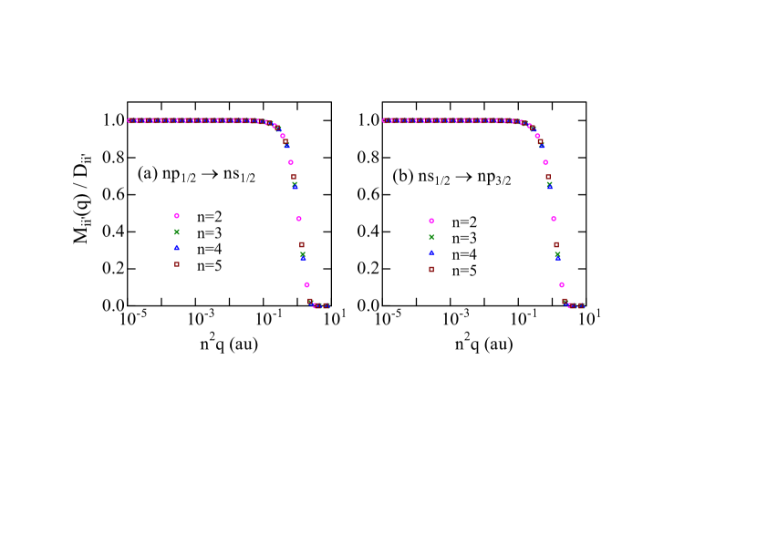
Figure 1: Values of $M_{{\rm ii}^{\prime}}(q)/D_{{\rm ii}^{\prime}}$ for the (a) $np_{1/2}\to ns_{1/2}$ and (b) $ns_{1/2}\to np_{3/2}$ transitions as functions of $n^{2}q$ ($n=2\sim 5$).

Figure 1 shows the values of $M_{{\rm ii}^{\prime}}(q)/D_{{\rm ii}^{\prime}}$ in (15) of (a) $np_{1/2}\to ns_{1/2}$ and (b) $ns_{1/2}\to np_{3/2}$ transitions as functions of $n^{2}q$ ($n=2\sim 5$). The value of $M_{{\rm ii}^{\prime}}(q)$ approaches that of $D_{{\rm ii}^{\prime}}$ for small $q$. The scaled curves for $n=2\sim 5$ are in good accordance. They begin to decrease around $n^{2}q\sim 0.1$ and are almost zero for $n^{2}q>1$. Similar behaviours are seen for the other transitions. Therefore, we have set the value of ${\bar{q}}_{\rm max}$ in (16) as

$$\begin{array}[]{c}{\bar{q}}_{\rm max}=\Biggl{\{}\begin{array}[]{ll}q_{\rm max}&q_{\rm max}\leq q_{1}\\ (q_{1}+q_{\rm max})/2&q_{1}<q_{\rm max}\leq q_{2}\\ q_{2}&q_{\rm max}>q_{2}\end{array}\end{array}$$ (21)

with $q_{1}=0.1/n^{2}$ and $q_{2}=1/n^{2}$.

3 Energy levels

As stated in Section 1, the energy differences between the fine-structure levels within (any) $n$ are very small for H and D. It is an important parameter for the optically allowed $nlj$–$nl^{\prime}j^{\prime}$ transitions. Energies for the levels of H and D have been taken from the NIST website https://physics.nist.gov/PhysRefData/HDEL/difftransfreq.html. These are also listed in Table 1a for a ready reference, where the energy of an $nlj$ is presented as difference from the $n$p_1/2 level, which is the lowest within an $n$ manifold. Though the binding energy of D($nlj$) is slightly larger than that of H($nlj$), due to the isotope shift, the energies listed in Table 1a for H are quite similar to those of D, and are specifically listed in Table 1b, in increasing order. This table also provides level indices for future references. It may be noted that the energy differences between $nlj$ and $nl^{\prime}j^{\prime}$ levels are also similar, and approximately scale as $1/n^{3}$ for both H and D.

4 Partial cross sections and collision strengths

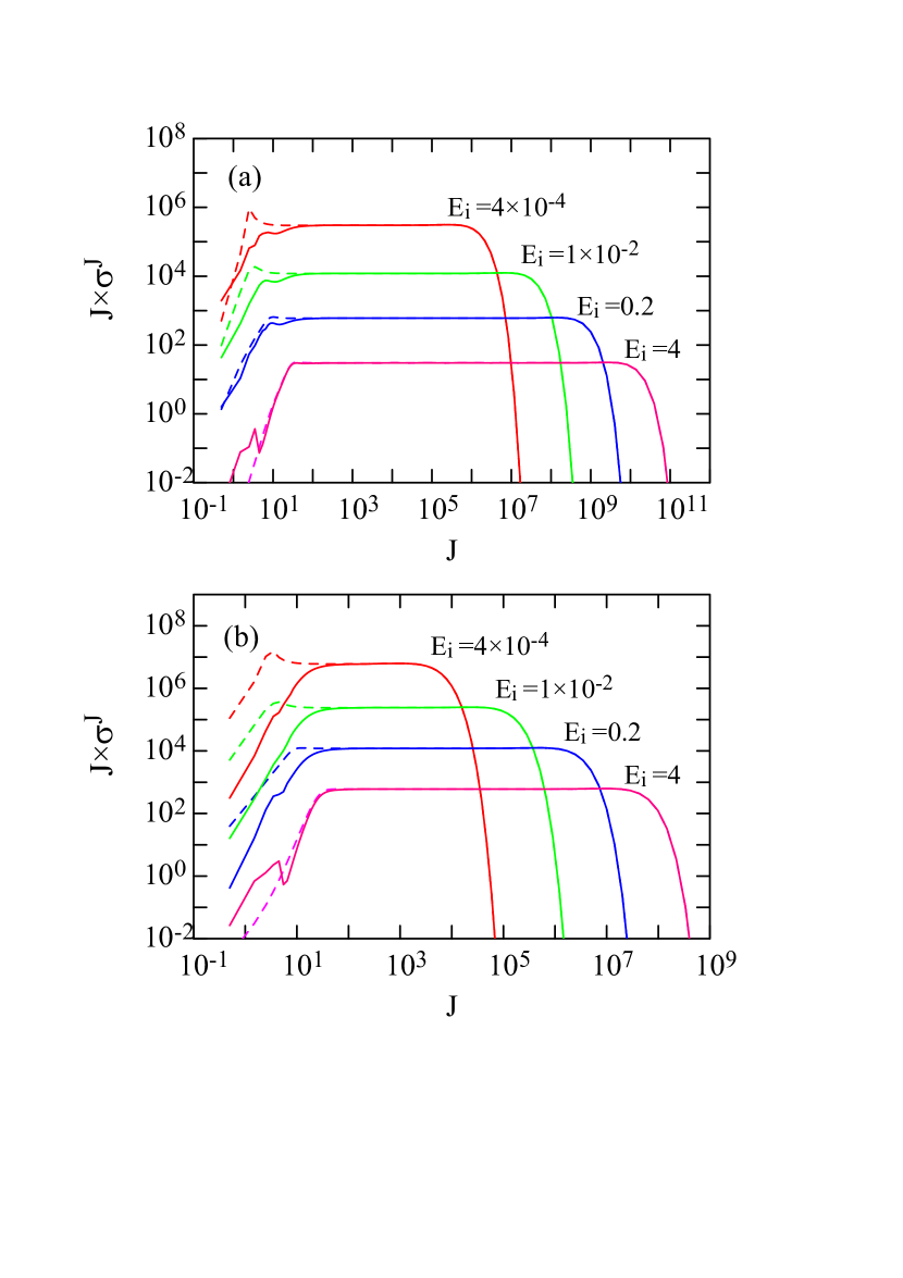
Figure 4: Variation of $J\times\sigma_{J}$ with partial waves $J$ for (a) 4f_5/2–4d_5/2 and (b) 4d_5/2–4f_7/2 transitions. Broken curves: Born and continuous curves: CC+Born results.

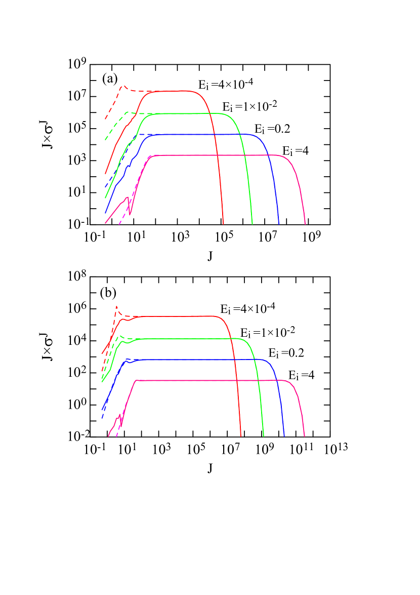
Figure 5: Variation of $J\times\sigma_{J}$ with partial waves $J$ for (a) 5d_5/2–5f_7/2 and (b) 5g_7/2–5f_7/2 transitions. Broken curves: Born and continuous curves: CC+Born results.

As examples, we show in Figures 2–5 the variation of $J\sigma^{J}$ with $J$ for two excitation transitions within $n$ = 2 ($i\to i^{\prime}$ = 2p_1/2 $\to$ 2s_1/2 and 2s_1/2 $\to$ 2p_3/2), 3 (3s_1/2 $\to$ 3p_3/2 and 3d_3/2 $\to$ 3p_3/2), 4 (4f_5/2 $\to$ 4d_5/2 and 4d_5/2 $\to$ 4f_7/2), and 5 (5d_5/2 $\to$ 5f_7/2 and 5g_7/2 $\to$ 5f_7/2), respectively, and at four incident energies of $E_{i}=k_{i}^{2}/2$ = 4$\times$10^-4, 1$\times$10^-2, 0.2, and 4 Ryd, which cover a wide range. Two sets of results are shown in these figures, i.e. Born (broken curves) and CC+Born (continuous curves). It is clear from these figures that the Born cross sections are overestimated at most energies (see also Figure 6), particularly for $J<$ 100, but above it there are (practically) no differences between the two sets of results. For this reason the CC results are only for $J<$ 100 and beyond these Born alone are used. The curves for $J\sigma^{J}$generally increase steeply with J at small values, then show plateaus at intermediate ones, and finally decrease exponentially for $J>J_{c}=\sqrt{k_{i}k_{i^{\prime}}}/|k_{i}-k_{i^{\prime}}|$, as equation (20) indicates. Note that $J_{c}\simeq E_{i}/(2\Delta\epsilon)$ for $E_{i}\gg\Delta\epsilon$, where $\Delta\epsilon=E_{i}-E_{i^{\prime}}$ is the excitation energy. As may be seen, particularly from Figure 5, that over 10¹¹ partial waves are required before $J\sigma^{J}$ starts decreasing. The values of $J\sigma^{J}$ at the plateau regions decrease as $1/E_{i}$ with $E_{i}$ in Figures 2–5.

In Table 2 we list our results for $\Omega$ for all 26 allowed fine structure transitions among the degenerate levels for $n=2\sim 5$ of H (given in Table 1b) in an energy range below 50 Ryd. Additionally, in Figure 6 we show the variation of $\Omega$ with energy for the optically allowed transitions within the $n=4$ manifold, as examples. The differences in the results obtained in the CC+Born and Born approximations gradually decrease with increasing energies, and almost disappear above $\sim$10 Ryd. A similar trend has been observed for other transitions as well. Finally, the Bethe-Born calculations in equation (16), for both $\sigma$ and $\Omega$, estimated by the three parameters $D_{ii^{\prime}}$, $q_{min}$ and $q_{max}$, reproduce well the corresponding results in the Born approximation.

Our $\Omega$ results, in both the CC+Born and Born approximations, for D are also included in Figure 6. However, these are very close to the corresponding results for H, and hence the differences between the two are negligible.

5 Effective collision strengths

The values of $\Omega$ listed in Table 2 are averaged over the Maxwellian distribution of electron velocities to obtain the effective collision strengths $\Upsilon$ as follows:

$$\Upsilon(T_{e})=\int_{0}^{\infty}{\Omega}(E_{i^{\prime}}(E_{i}))\,{\rm exp}(-E_{i^{\prime}}/kT_{e})\,d(E_{i^{\prime}}/{kT_{e}}),$$ (22)

where $k$ is Boltzmann constant, $T_{e}$ is the electron temperature in K, and $E_{i^{\prime}}$ is the electron energy with respect to the final (excited) state/level. This value of $\Upsilon$ is related to the excitation $q(i,i^{\prime})$ and de-excitation $q(i^{\prime},i)$ rates as follows:

$$q(i,i^{\prime})=\frac{8.63\times 10^{-6}}{{\omega_{i}}{T_{e}^{1/2}}}\Upsilon\,{\rm exp}(-\Delta\epsilon/{kT_{e}})\hskip 28.45274pt{\rm cm^{3}s^{-1}}$$ (23)

and

$$q(i^{\prime},i)=\frac{8.63\times 10^{-6}}{{\omega_{i^{\prime}}}{T_{e}^{1/2}}}\Upsilon\hskip 28.45274pt{\rm cm^{3}s^{-1}},$$ (24)

where $\omega_{i}$ and $\omega_{i^{\prime}}$ are the statistical weights of the initial ($i$) and final ($i^{\prime}$) states, respectively, and $\Delta\epsilon=E_{i}-E_{i^{\prime}}$ is the excitation energy. We have used the $\Omega(E_{i})$ values in the CC+Born approximation for $E_{i}\leq 20$ Ryd in equation (22), but in Born (equation (15)) alone above it, and up to an energy of 1000 Ryd. Results for these rates are required in the modeling and diagnostics of plasmas. The calculated values of $\Upsilon$ are listed in Table 3 for all 26 transitions and at a wide temperature range, up to 10⁷ K, suitable for applications in a variety of plasmas, including fusion. Furthermore, the variation of $\Upsilon$ with $T_{e}$ is rather smooth, as between 10³ and 10⁷ K it varies by a maximum factor of 2.2 for a few transitions, and much less for most. Therefore, values of $\Upsilon$ at any desired $T_{e}$ within this range can be easily interpolated without any loss of accuracy.

In the absence of any other similar results in the literature, either for $\Omega$ or $\Upsilon$, it is difficult to assess the accuracy of our calculated data, particularly when the calculations are very sensitive to $\Delta\epsilon$, as noted in Section 1. In the past, for several ions we have performed calculations with FAC to make some estimation of the accuracy of data – see for example, Hamada et al.  [10] for O VIII and Ni XXVIII and Aggarwal et al.  [15] for He II. However, similar calculations performed for H have been highly unsatisfactory, because for some transitions, such as 5–6 (3p_1/2–3s_1/2), 8–9 (3p_3/2–3d_5/2) and 10–12 (4p_1/2–4d_3/2), values of $\Omega$ decrease with increasing energy, whereas for others, such as 7–8 (3d_3/2–3p_3/2) and 10–11 (4p_1/2–4s_1/2), they suddenly increase by up to six orders of magnitude. Therefore, these calculations cannot be relied upon for comparison or accuracy assessment, and it confirms yet again that although FAC is very efficient for generating large amount of atomic data with (normally) some measure of accuracy, it is not designed to produce sophisticated results for higher accuracy. Nevertheless, in the near future we plan to make a detailed analysis of population modelling for fusion (tokamak) plasmas, on a similar line as recently done for He II (Lawson et al.  [12]), and that may give some idea of the accuracy of the reported data.

Finally, we have (mostly) presented results for the transitions of H, but calculations have also been performed for all transitions of D. However, there are negligible differences ($<$ 1%) between the two sets of results, for both $\Omega$ and $\Upsilon$, because $\Delta\epsilon$ among the levels of H and D differ by no more than $\sim$ 0.15%. Therefore, we can confidently state that the same results as listed in Tables 2 and 3 can be reliably applied for both H and D.

6 Conclusions

In this paper we have presented results for 26 transitions of H which are allowed within the degenerate levels of states with $n\leq$ 5. Results have been listed for both $\Omega$ and $\Upsilon$ over a wide energy/temperature range, and will not only be helpful for the modelling of plasmas, but also for future comparisons, because no such data presently exist in the literature. The listed results also complement our earlier data (Aggarwal et al.  [5]) and are required for considering a complete plasma model for fusion studies. Additionally, parallel calculations have also been performed for D, but the results are insignificantly different from those for H. This is an important conclusion for future studies.

Figure 6: Variation of $\Omega$ with energy $E_{i}$ for the transitions within $n$ = 4. (a) 4p_1/2–4s_1/2, (b) 4p_1/2–4d_3/2, (c) 4s_1/2–4p_3/2, (d) 4d_3/2–4p_3/2, (e) 4d_3/2–4f_5/2, (f) 4p_3/2–4d_5/2, (g) 4f_5/2–4d_5/2 and (h) 4d_5/2–4f_7/2. Upper and lower curves are for Born and CC+Born collision strengths for H (continuous curves) and D (dots). Circles on upper curves are Bethe-Born results for H.

Table 1: a. Energies (Ryd) for the levels of atomic hydrogen and deuterium with respect to the $n$p_1/2 level. $a{\pm}b\equiv a{\times}$10^±b.

$n$	Level	H	D
2	2p1/2	0.000000+0	0.000000+0
	2s1/2	3.215489$-$7	3.219711$-$7
	2p3/2	3.334219$-$6	3.335129$-$6
3	3p1/2	0.000000+0	0.000000+0
	3s1/2	9.571226$-$8	9.583735$-$8
	3d3/2	9.862969$-$7	9.865650$-$7
	3p3/2	9.879176$-$7	9.881873$-$7
	3d5/2	1.315595$-$6	1.315953$-$6
4	4p1/2	0.000000+0	0.00000+0
	4s1/2	4.045105$-$8	4.050383$-$8
	4d3/2	4.160819$-$7	4.161950$-$7
	4p3/2	4.167772$-$7	4.168910$-$7
	4f5/2	5.547586$-$7	5.549094$-$7
	4d5/2	5.550046$-$7	5.551556$-$7
	4f7/2	6.242196$-$7	6.243893$-$7
5	5p1/2	0.000000+0	0.000000+0
	5s1/2	2.072911$-$8	2.075613$-$8
	5d3/2	2.130304$-$7	2.130883$-$7
	5p3/2	2.133897$-$7	2.134479$-$7
	5f5/2	2.840319$-$7	2.841091$-$7
	5d5/2	2.841589$-$7	2.842362$-$7
	5g7/2	3.195295$-$7	3.196164$-$7
	5f7/2	3.195959$-$7	3.196829$-$7
	5g9/2	3.408679$-$7	3.409606$-$7

Table 1: b. Energy levels (Ryd) of atomic hydrogen and deuterium.

Index	Level	H	D
1	1s1/2	0.000 000 000 000	0.000 000 000 000
2	2p1/2	0.749 598 426 021	0.749 802 385 029
3	2s1/2	0.749 598 747 570	0.749 802 707 000
4	2p3/2	0.749 601 760 240	0.749 805 720 158
5	3p1/2	0.888 414 397 520	0.888 656 128 310
6	3s1/2	0.888 414 493 232	0.888 656 224 147
7	3d3/2	0.888 415 383 817	0.888 657 114 875
8	3p3/2	0.888 415 385 438	0.888 657 116 497
9	3d5/2	0.888 415 713 115	0.888 657 444 263
10	4p1/2	0.936 999 852 243	0.937 254 802 720
11	4s1/2	0.936 999 892 694	0.937 254 843 224
12	4d3/2	0.937 000 268 325	0.937 255 218 915
13	4p3/2	0.937 000 269 020	0.937 255 219 611
14	4f5/2	0.937 000 407 002	0.937 255 357 629
15	4d5/2	0.937 000 407 248	0.937 255 357 876
16	4f7/2	0.937 000 476 463	0.937 255 427 109
17	5p1/2	0.959 487 919 100	0.959 748 987 500
18	5s1/2	0.959 487 939 829	0.959 749 008 256
19	5d3/2	0.959 488 132 130	0.959 749 200 588
20	5p3/2	0.959 488 132 490	0.959 749 200 948
21	5f5/2	0.959 488 203 132	0.959 749 271 609
22	5d5/2	0.959 488 203 259	0.959 749 271 736
23	5g7/2	0.959 488 238 630	0.959 749 307 116
24	5f7/2	0.959 488 238 696	0.959 749 307 183
25	5g9/2	0.959 488 259 968	0.959 749 328 461

Table 2: Collision strengths for transitions of atomic hydrogen as a function of energy. $a{\pm}b\equiv a{\times}$10^±b.

$E_{i}$ (Ryd)	Transition
I	2: 2p1/2	3: 2s1/2	5: 3p1/2	5: 3p1/2	6: 3s1/2	7: 3d3/2	8: 3p3/2	10: 4p1/2	10: 4p1/2
J	3: 2s1/2	4: 2p3/2	6: 3s1/2	7: 3d3/2	8: 3p3/2	8: 3p3/2	9: 3d5/2	11: 4s1/2	12: 4d3/2
2.0$-$04	2.328+2	3.172+2	1.462+3	1.201+3	1.756+3	7.185+2	2.673+3	5.089+3	4.691+3
4.0$-$04	2.692+2	3.463+2	1.670+3	1.324+3	2.026+3	7.708+2	3.122+3	5.759+3	5.747+3
1.0$-$03	3.120+2	4.039+2	1.927+3	1.654+3	2.549+3	8.435+2	3.753+3	6.637+3	7.238+3
2.0$-$03	3.438+2	4.674+2	2.131+3	1.919+3	2.979+3	8.862+2	4.204+3	7.308+3	8.314+3
4.0$-$03	3.854+2	5.397+2	2.335+3	2.172+3	3.384+3	9.386+2	4.642+3	7.976+3	9.383+3
1.0$-$02	4.316+2	6.697+2	2.598+3	2.573+3	3.896+3	1.012+3	5.246+3	8.855+3	1.078+4
2.0$-$02	4.559+2	6.971+2	2.800+3	2.748+3	4.311+3	1.067+3	5.693+3	9.517+3	1.185+4
4.0$-$02	4.877+2	7.758+2	3.000+3	3.000+3	4.711+3	1.114+3	6.140+3	1.018+4	1.292+4
1.0$-$01	5.313+2	8.852+2	3.259+3	3.368+3	5.233+3	1.174+3	6.735+3	1.106+4	1.432+4
2.0$-$01	5.736+2	9.148+2	3.459+3	3.578+3	5.632+3	1.222+3	7.247+3	1.172+4	1.538+4
4.0$-$01	6.063+2	9.805+2	3.655+3	3.824+3	6.024+3	1.270+3	7.619+3	1.238+4	1.642+4
1.0$+$00	6.471+2	1.080+3	3.909+3	4.125+3	6.529+3	1.331+3	8.161+3	1.324+4	1.778+4
2.0$+$00	6.742+2	1.133+3	4.081+3	4.368+3	6.875+3	1.350+3	8.523+3	1.385+4	1.872+4
4.0$+$00	6.891+2	1.180+3	4.236+3	4.587+3	7.184+3	1.381+3	8.910+3	1.437+4	1.998+4
1.0$+$01	7.165+2	1.235+3	4.412+3	4.714+3	7.534+3	1.444+3	9.206+3	1.496+4	2.053+4
2.0$+$01	7.376+2	1.260+3	4.541+3	4.863+3	7.796+3	1.448+3	9.477+3	1.541+4	2.114+4
3.0$+$01	7.474+2	1.280+3	4.599+3	4.936+3	7.912+3	1.462+3	9.608+3	1.560+4	2.145+4
4.0$+$01	7.543+2	1.294+3	4.641+3	4.988+3	7.955+3	1.473+3	9.701+3	1.574+4	2.167+4
5.0$+$01	7.596+2	1.304+3	4.673+3	5.028+3	8.059+3	1.481+3	9.773+3	1.585+4	2.184+4

Table 2: continued.

$E_{i}$ (Ryd)	Transition
I	11: 4s1/2	12: 4d3/2	12: 4d3/2	13: 4p3/2	14: 4f5/2	15: 4d5/2	17: 5p1/2	17: 5p1/2	18: 5s1/2
J	13: 4p3/2	13: 4p3/2	14: 4f5/2	15: 4d5/2	15: 4d5/2	16: 4f7/2	18: 5s1/2	19: 5d3/2	20: 5p3/2
2.0$-$04	5.816+3	3.030+3	7.301+3	1.163+4	1.341+3	1.210+4	1.318+4	1.338+4	1.543+4
4.0$-$04	7.134+3	3.242+3	8.439+3	1.360+4	1.426+3	1.372+4	1.485+4	1.632+4	1.882+4
1.0$-$03	8.935+3	3.523+3	9.944+3	1.617+4	1.527+3	1.581+4	1.707+4	2.023+4	2.327+4
2.0$-$03	1.033+4	3.736+3	1.104+4	1.804+4	1.608+3	1.743+4	1.874+4	2.328+4	2.664+4
4.0$-$03	1.163+4	3.952+3	1.217+4	1.998+4	1.688+3	1.904+4	2.040+4	2.619+4	3.005+4
1.0$-$02	1.342+4	4.232+3	1.366+4	2.253+4	1.790+3	2.114+4	2.259+4	3.006+4	3.447+4
2.0$-$02	1.475+4	4.449+3	1.478+4	2.447+4	1.870+3	2.275+4	2.426+4	3.297+4	3.782+4
4.0$-$02	1.608+4	4.658+3	1.590+4	2.638+4	1.946+3	2.434+4	2.591+4	3.589+4	4.113+4
1.0$-$01	1.784+4	4.937+3	1.737+4	2.890+4	2.050+3	2.643+4	2.810+4	3.973+4	4.552+4
2.0$-$01	1.917+4	5.149+3	1.847+4	3.080+4	2.128+3	2.802+4	2.976+4	4.260+4	4.882+4
4.0$-$01	2.050+4	5.358+3	1.955+4	3.267+4	2.196+3	2.956+4	3.140+4	4.548+4	5.211+4
1.0$+$00	2.221+4	5.616+3	2.089+4	3.512+4	2.273+3	3.147+4	3.355+4	4.924+4	5.647+4
2.0$+$00	2.342+4	5.789+3	2.180+4	3.681+4	2.324+3	3.275+4	3.510+4	5.188+4	5.954+4
4.0$+$00	2.457+4	5.943+3	2.265+4	3.924+4	2.391+3	3.451+4	3.644+4	5.456+4	6.282+4
1.0$+$01	2.585+4	6.117+3	2.381+4	3.990+4	2.437+3	3.535+4	3.794+4	5.675+4	6.602+4
2.0$+$01	2.654+4	6.249+3	2.411+4	4.113+4	2.475+3	3.606+4	3.906+4	5.867+4	6.741+4
3.0$+$01	2.693+4	6.311+3	2.444+4	4.169+4	2.498+3	3.652+4	3.954+4	5.952+4	6.839+4
4.0$+$01	2.720+4	6.355+3	2.467+4	4.209+4	2.515+3	3.685+4	3.989+4	6.013+4	6.908+4
5.0$+$01	2.742+4	6.390+3	2.485+4	4.240+4	2.528+3	3.711+4	4.016+4	6.059+4	6.961+4

Table 2: continued.

$E_{i}$ (Ryd)	Transition
I	19: 5d3/2	19: 5d3/2	20: 5p3/2	21: 5f5/2	21: 5f5/2	22: 5d5/2	23: 5g7/2	24: 5f7/2
J	20: 5p3/2	21: 5f5/2	22: 5d5/2	22: 5d5/2	23: 5g7/2	24: 5f7/2	24: 5f7/2	25: 5g9/2
2.0$-$04	8.346+3	2.564+4	3.257+4	4.626+3	2.574+4	4.290+4	2.184+3	3.652+4
4.0$-$04	8.925+3	2.992+4	3.825+4	4.908+3	2.886+4	4.843+4	2.307+3	4.064+4
1.0$-$03	9.696+3	3.518+4	4.505+4	5.289+3	3.319+4	5.613+4	2.454+3	4.618+4
2.0$-$03	1.028+4	3.923+4	5.038+4	5.579+3	3.642+4	6.190+4	2.574+3	5.034+4
4.0$-$03	1.086+4	4.326+4	5.567+4	5.856+3	3.965+4	6.761+4	2.695+3	5.449+4
1.0$-$02	1.162+4	4.856+4	6.261+4	6.235+3	4.388+4	7.515+4	2.851+3	6.000+4
2.0$-$02	1.221+4	5.256+4	6.785+4	6.530+3	4.712+4	8.086+4	2.964+3	6.417+4
4.0$-$02	1.279+4	5.656+4	7.308+4	6.811+3	5.027+4	8.652+4	3.085+3	6.830+4
1.0$-$01	1.356+4	6.179+4	7.996+4	7.187+3	5.449+4	9.407+4	3.234+3	7.375+4
2.0$-$01	1.415+4	6.575+4	8.515+4	7.468+3	5.766+4	9.971+4	3.341+3	7.785+4
4.0$-$01	1.472+4	6.970+4	9.037+4	7.746+3	6.073+4	1.053+5	3.435+3	8.184+4
1.0$+$00	1.546+4	7.474+4	9.715+4	8.080+3	6.456+4	1.126+5	3.545+3	8.677+4
2.0$+$00	1.595+4	7.827+4	1.019+5	8.306+3	6.707+4	1.176+5	3.619+3	9.002+4
4.0$+$00	1.639+4	8.126+4	1.060+5	8.507+3	6.963+4	1.219+5	3.753+3	9.284+4
1.0$+$01	1.688+4	8.461+4	1.106+5	8.734+3	7.172+4	1.266+5	3.794+3	9.607+4
2.0$+$01	1.725+4	8.713+4	1.140+5	8.905+3	7.358+4	1.302+5	3.837+3	9.847+4
3.0$+$01	1.742+4	8.830+4	1.156+5	8.989+3	7.452+4	1.319+5	3.872+3	9.968+4
4.0$+$01	1.755+4	8.913+4	1.167+5	9.048+3	7.519+4	1.331+5	3.897+3	1.005+5
5.0$+$01	1.764+4	8.977+4	1.175+5	9.094+3	7.570+4	1.340+5	3.916+3	1.012+5

Table 3: Effective collision strengths for transitions of atomic hydrogen as function of temperature. $a{\pm}b\equiv a{\times}$10^±b.

$\log_{10}T_{e}$ (K)	Transition
I	2: 2p1/2	3: 2s1/2	5: 3p1/2	5: 3p1/2	6: 3s1/2	7: 3d3/2	8: 3p3/2	10: 4p1/2	10: 4p1/2
J	3: 2s1/2	4: 2p3/2	6: 3s1/2	7: 3d3/2	8: 3p3/2	8: 3p3/2	9: 3d5/2	11: 4s1/2	12: 4d3/2
3.00	4.100+2	6.121+2	2.500+3	2.403+3	3.713+3	9.859+2	5.021+3	8.526+3	1.026+4
3.33	4.447+2	6.862+2	2.719+3	2.672+3	4.150+3	1.042+3	5.513+3	9.254+3	1.143+4
3.66	4.802+2	7.611+2	2.938+3	2.944+3	4.588+3	1.096+3	6.010+3	9.982+3	1.260+4
4.00	5.188+2	8.327+2	3.162+3	3.222+3	5.037+3	1.151+3	6.525+3	1.073+4	1.380+4
4.33	5.567+2	9.003+2	3.378+3	3.486+3	5.470+3	1.203+3	7.011+3	1.146+4	1.495+4
4.66	5.931+2	9.697+2	3.590+3	3.746+3	5.896+3	1.253+3	7.476+3	1.217+4	1.609+4
5.00	6.272+2	1.040+3	3.801+3	4.011+3	6.316+3	1.298+3	7.932+3	1.289+4	1.726+4
5.33	6.556+2	1.102+3	3.990+3	4.250+3	6.695+3	1.338+3	8.345+3	1.354+4	1.835+4
5.66	6.809+2	1.156+3	4.164+3	4.453+3	7.042+3	1.377+3	8.712+3	1.413+4	1.930+4
6.00	7.051+2	1.204+3	4.325+3	4.634+3	7.366+3	1.411+3	9.045+3	1.468+4	2.012+4
6.33	7.268+2	1.244+3	4.466+3	4.792+3	7.647+3	1.439+3	9.337+3	1.515+4	2.082+4
6.66	7.471+2	1.282+3	4.592+3	4.940+3	7.901+3	1.466+3	9.608+3	1.558+4	2.146+4
7.00	7.666+2	1.320+3	4.712+3	5.084+3	8.142+3	1.493+3	9.871+3	1.598+4	2.208+4
	11: 4s1/2	12: 4d3/2	12: 4d3/2	13: 4p3/2	14: 4f5/2	15: 4d5/2	17: 5p1/2	17: 5p1/2	18: 5s1/2
$\log_{10}T_{e}$ (K)	13: 4p3/2	13: 4p3/2	14: 4f5/2	15: 4d5/2	15: 4d5/2	16: 4f7/2	18: 5s1/2	19: 5d3/2	20: 5p3/2
3.00	1.276+4	4.128+3	1.311+4	2.159+4	1.751+3	2.036+4	2.177+4	2.862+4	3.282+4
3.33	1.422+4	4.361+3	1.433+4	2.370+4	1.837+3	2.211+4	2.360+4	3.182+4	3.648+4
3.66	1.568+4	4.594+3	1.556+4	2.580+4	1.923+3	2.385+4	2.541+4	3.501+4	4.012+4
4.00	1.718+4	4.832+3	1.681+4	2.795+4	2.010+3	2.564+4	2.728+4	3.828+4	4.387+4
4.33	1.864+4	5.062+3	1.801+4	3.003+4	2.091+3	2.736+4	2.909+4	4.145+4	4.750+4
4.66	2.007+4	5.285+3	1.917+4	3.208+4	2.166+3	2.902+4	3.088+4	4.458+4	5.110+4
5.00	2.151+4	5.502+3	2.031+4	3.419+4	2.237+3	3.069+4	3.268+4	4.774+4	5.477+4
5.33	2.284+4	5.695+3	2.136+4	3.617+4	2.301+3	3.224+4	3.432+4	5.062+4	5.822+4
5.66	2.406+4	5.870+3	2.231+4	3.786+4	2.358+3	3.358+4	3.581+4	5.322+4	6.136+4
6.00	2.516+4	6.034+3	2.315+4	3.931+4	2.410+3	3.471+4	3.720+4	5.558+4	6.410+4
6.33	2.608+4	6.177+3	2.384+4	4.055+4	2.457+3	3.568+4	3.840+4	5.760+4	6.636+4
6.66	2.691+4	6.308+3	2.448+4	4.170+4	2.502+3	3.659+4	3.948+4	5.944+4	6.839+4
7.00	2.770+4	6.433+3	2.512+4	4.282+4	2.546+3	3.749+4	4.049+4	6.119+4	7.035+4

Table 3: continued.

$\log_{10}T_{e}$ (K)	Transition
I	19: 5d3/2	19: 5d3/2	20: 5p3/2	21: 5f5/2	21: 5f5/2	22: 5d5/2	23: 5g7/2	24: 5f7/2
J	20: 5p3/2	21: 5f5/2	22: 5d5/2	22: 5d5/2	23: 5g7/2	24: 5f7/2	24: 5f7/2	25: 5g9/2
3.00	1.134+4	4.657+4	6.001+4	6.097+3	4.230+4	7.234+4	2.791+3	5.795+4
3.33	1.198+4	5.096+4	6.576+4	6.411+3	4.581+4	7.859+4	2.920+3	6.250+4
3.66	1.262+4	5.534+4	7.149+4	6.724+3	4.931+4	8.483+4	3.046+3	6.704+4
4.00	1.328+4	5.982+4	7.738+4	7.044+3	5.290+4	9.124+4	3.172+3	7.168+4
4.33	1.391+4	6.415+4	8.309+4	7.350+3	5.633+4	9.743+4	3.287+3	7.613+4
4.66	1.453+4	6.841+4	8.874+4	7.645+3	5.964+4	1.035+5	3.393+3	8.042+4
5.00	1.514+4	7.262+4	9.436+4	7.930+3	6.288+4	1.095+5	3.498+3	8.455+4
5.33	1.569+4	7.639+4	9.943+4	8.183+3	6.576+4	1.149+5	3.598+3	8.819+4
5.66	1.618+4	7.980+4	1.040+5	8.411+3	6.829+4	1.198+5	3.684+3	9.146+4
6.00	1.664+4	8.296+4	1.084+5	8.625+3	7.060+4	1.243+5	3.756+3	9.451+4
6.33	1.704+4	8.571+4	1.120+5	8.813+3	7.264+4	1.282+5	3.819+3	9.720+4
6.66	1.741+4	8.821+4	1.154+5	8.988+3	7.455+4	1.318+5	3.882+3	9.970+4
7.00	1.776+4	9.059+4	1.186+5	9.154+3	7.641+4	1.352+5	3.946+3	1.021+5

References

- [1] Kramida, A.E. A critical compilation of experimental data on spectral lines and energy levels of hydrogen, deuterium, and tritium. At. Data Nucl. Data Tables 2010, 96, 586-644.
- [2] Wiese, W.L.; Fuhr, J.R. Accurate atomic transition probabilities for hydrogen, helium, and lithium. J. Phys. Chem. Ref. Data 2009, 38, 565-726 + 1129.
- [3] Anderson, H.; Ballance, C.P.; Badnell, N.R.; Summers, H.P. An R-matrix with pseudostates approach to the electron-impact excitation of H I for diagnostic applications in fusion plasmas. J. Phys. B 2000, 33, 1255-1262.
- [4] Benda, J.; Houfek, K. Converged and consistent high-resolution low-energy electron-hydrogen scattering. I. Data below = 4 threshold for applications in stellar physics. 2018 At. Data Nucl. Data Tables 119, 303-313.
- [5] Aggarwal, K.M.; Berrington, K.A.; Burke, P.G.; Kingston, A.E.; Pathak, A. Electron collision cross sections at low energies for all transitions between the =1, 2, 3, 4 and 5 levels of atomic hydrogen. J. Phys. B, 1991, 24, 1385-1410.
- [6] Henry, R.J.W. Excitation of atomic positive ions by electron impact. Phys. Rept. 1981, 68, 1-91.
- [7] Anderson, H.; Ballance, C.P.; Badnell, N.R; Summers, H.P. Corrigendum: An R-matrix with pseudostates approach to the electron-impact excitation of H I for diagnostic applications in fusion plasmas. J. Phys. B 2002, 35, 1613-1615.
- [8] Lavrov, B.P.; Pipa, A.V. Account of the fine structure of hydrogen atom levels in the effective emission cross sections of Balmer lines excited by electron impact in gases and plasma. Opt. Spect. 2002, 92, 647-657.
- [9] Wünderlich, D.; Dietrich, S.; Fantz, U. Application of a collisional radiative model to atomic hydrogen for diagnostic purposes. J. Quant. Spect. Rad. Transf. 2009, 110, 62-71.
- [10] Hamada, K.; Aggarwal, K.M.; Akita, K.; Igarashi, A.; Keenan, F.P.; Nakazaki, S. Effective collision strengths for optically allowed transitions among degenerate levels of hydrogenic ions with 2 Z 30. At. Data Nucl. Data Tables 2010, 96, 481-530.
- [11] Gu, M.F. The flexible atomic code. Can. J. Phys. 2008, 86, 675–689.
- [12] Lawson, K.D.; Aggarwal, K.M.; Coffey, I.H.; Keenan, F.P.; O’Mullane, M.G.; JET-EFDA Contributors. Population modelling of the He II energy levels in tokamak plasmas. I : Collisional excitation model. J. Phys. B 2018, 51 - to be submitted.
- [13] Igarashi, A., Horiguchi, Y., Ohsaki, A., Nakazaki, S. Electron-impact excitations between the = 2 fine-structure levels of hydrogenic ions. J. Phys. Soc. Japan 2003, 72 307-312.
- [14] Igarashi, A.; Ohsaki, A.; Nakazaki. S. Electron-exchange effect in electron-impact excitation of the = 2 fine-structure levels of hydrogenic ions. J. Phys. Soc. Japan 2005, 74, 321-325.
- [15] Aggarwal, K.M.; Igarashi, A.; Keenan, F.P.; Nakazaki, S. Radiative rates and electron impact excitation rates for transitions in He II. Atoms 2017, 5, 19.
- [16] Alder, K.; Bohr, A., Huus, T.; Mottelson, B.; Winther, A. Study of nuclear structure by electromagnetic excitation with accelerated ions. Rev. Mod. Phys. 1956, 28, 432-542.
- [17] Alder, K.; Bohr, A.; Huus, T.; Mottelson, B.; Winther, A. Errata: Study of nuclear structure by electromagnetic excitation with accelerated ions. Rev. Mod. Phys. 1958, 30, 353.