Abstract

This paper focuses on modeling the dynamic attributes of a dynamic network with a fixed number of vertices. These attributes are considered as time series which dependency structure is influenced by the underlying network. They are modeled by a multivariate doubly stochastic time series framework, that is we assume linear processes for which the coefficient matrices are stochastic processes themselves. We explicitly allow for dependence in the dynamics of the coefficient matrices as well as between these two stochastic processes. This framework allows for a separate modeling of the attributes and the underlying network. In this setting, we define network autoregressive models and discuss their stationarity conditions. Furthermore, an estimation approach is discussed in a low- and high-dimensional setting and how this can be applied to forecasting. The finite sample behavior of the forecast approach is investigated. This approach is applied to real data whereby the goal is to forecast the GDP of $33$ economies.

1 Introduction

Consider a vertex-labeled dynamic and weighted network with a fixed number $d$ of vertices given by the set $V=\{1,\dots,d\}$. The weights are within the interval $[-1,1]$. Such a dynamic and weighted network with a fixed number of vertices can be described by a time dependent adjacency matrix, here denoted by $\mathbf{Ad}=\{Ad_{t},t\in\mathds{Z}\}$, where $Ad_{t}$ is $[-1,1]^{d\times d}$- valued. If no edge is present at time $t$, a zero weight is considered. Thus, $e_{i}^{\top}Ad_{t}e_{j}$ gives the weight of an edge at time $t$ from vertex $i$ to vertex $j$. It is considered that the network is driven by some random process, hence, the corresponding adjacency matrix process $\mathbf{Ad}$ is a stochastic process.

The vertices are considered as actors (e.g. people, countries), and a network could describe a relationship structure among these actors. A (weighted) edge between two actors describes some connection between them. The weights can be interpreted as the strength of the connection. For example, consider economies as actors where a possible relationship between two economies could be given by their relative trade volume at a given time point. Further examples are social networks, see [10, 23]. The actors in such networks often possess attributes. These attributes can be static (e.g a person’s name or birthday) or dynamic (e.g. personal income, time a person does sports, or political views). In the example with the economies and their trade volume as a relationship between them, dynamic attributes of interest are macroeconomic measures such as inflation rate or gross domestic product (GDP). These attributes may be affected by the attributes of other actors, especially by actors with which the considered actor is strongly connected. In this work, the dynamic attributes are denoted by a time series $\mathbf{X}=\{X_{t},t\in\mathds{Z}\}$. To simplify the notation, we focus on the case that each actor has only one attribute, meaning that $\mathbf{X}$ is d-dimensional. Nevertheless, this framework can also handle multiple attributes per actor, see Section 2 for details.

In this work, the dynamic attributes are denoted by a $d$-dimensional time series $\mathbf{X}=\{X_{t},t\in\mathds{Z}\}$, where each component of the time series is assigned to a vertex (actor) of the underlying network. In the social-economical literature, the influence of connected actors on the attributes is denoted as peer effect, see [8, 20].

This work focuses on the dynamic attributes and not on the network itself. Consequently, this work is not about modeling a dynamic network. For modeling these dynamic networks, many models for static networks have been extended to the dynamic case as done by [9, 15] for the Exponential Random Graph Models (ERGM), see Section 6.5 in [14], or by [38, 39] for the stochastic block model (SBM). By contrast, this work gives a framework which models the dynamic attributes, that means modeling a time series on a dynamic network, in which the weighted edges influence the dependency of the time series. [12, 42] have modeled these attributes for non-random edges, which mainly cover static networks. In the context of a static network, attributes can be considered as standard multivariate time series with additional information and can be modeled by using vector autoregressive (VAR) models with constraints, see Lütkepohl, [19, Chapter 2 and 5]. However, VAR models have many parameters, which is why [12, 42] focus on how to use the network structure to reduce the number of parameters so that high dimensions, meaning a large number of vertices, become feasible. By contrast, this work deals with a random network structure, and consequently, the process $\mathbf{X}$ cannot be modeled appropriately by using VAR models. Instead, we adopt a multivariate doubly stochastic time series framework, meaning two stochastic processes drive the time series. On the one hand, there is the innovation process of the time series. On the other hand, the coefficient matrices in linear processes or autoregressive models are stochastic processes themselves. Doubly stochastic time series models were introduced in Tjøstheim, [31], Pourahmadi, [27, 28], and these authors assume that the two processes driving the time series are independent. That would mean the network could influence the attributes but not the other way around. This assumption could be too restrictive for most application. In the example where the GDP is the attribute and the trade volume defines the underlying network, the influence goes in both directions. To capture such behavior, we allow dependency between both processes, see Section 2 for details. Hence, the network, in form of the edges, can influence the attributes, and the attributes can influence the edges.

Knight et al., [11] extended the model of [12] to dynamic networks. Their model can be considered as a special case of the model considered in this paper, see Section 2 for details. They present an R-package to estimate their model, however, they present theoretical results only for the case of a static network such that the attributes can be written as a VAR model with constraints. Thus, they do not derive theoretical results for the dynamic case. This gap is filled in this work.

This paper is structured as follows. In Section 2, time series on dynamic networks are defined and some basic properties are given. In Section 3, the focus is on statistical results of network autoregressive processes, and their applications to forecasting are discussed. Some of the forecasting results are underlined by a simulation study which is given in Section 4. In Section 5, we apply this setup to forecast the GDP using the trade volume between economies as an underlying network. Proofs can be found in Section 7.

2 Time Series Modeling on Dynamic Networks

To elaborate, we first fix some notation. For a random variable $X$, we write $\|X\|_{E,q}$ for $\big{(}E|X|^{q}\big{)}^{1/q}$, where $q\in\mathds{N}$; for a vector $x\in\mathds{R}^{d}$, $\|x\|_{0}=\sum_{j=1}^{d}\mathds{1}(x_{j}\not=0)$, $\|x\|_{1}=\sum_{j=1}^{d}|x_{j}|$ and $\|x\|_{2}^{2}=\sum_{j=1}^{d}|x_{j}|^{2}$. Furthermore, for a $r\times s$ matrix $B=(b_{i,j})_{i=1,\ldots,r,j=1,\ldots,s}$, $\|B\|_{1}=\max_{1\leq j\leq s}\sum_{i=1}^{r}|b_{i,j}|=\max_{j}\|Be_{j}\|_{1}$, $\|B\|_{\infty}=\max_{1\leq i\leq r}\sum_{j=1}^{s}|b_{i,j}|=\max_{i}\|e_{i}^{\top}B\|_{1}$, $\|B\|_{\max}=\max_{i,j}|e_{i}^{\top}Be_{j}|$, where $e_{j}=(0,\ldots,0,1,0,\ldots,0)^{\top}$ denotes the vector with the one appearing in the $j$th position. Let $\mathds{1}=(1,\dots,1)^{\top}$ be a vector of ones. For a matrix $B$, the absolute value evaluated component-wise is denoted by $|B|$. Denote the largest eigenvalue of a matrix $B$ by $\rho(B)$ and $\|B\|_{2}^{2}=\rho(BB^{\top})$. The $d$-dimensional identity matrix is denoted by $I_{d}$. Furthermore, for two matrices $A,B$ the Kronecker product of $A$ and $B$ is denoted by $A\otimes B$, see among others Appendix A.11 in [19]. Let $A\odot B$ denote the component-wise multiplication of $A$ and $B$, i.e. the Hadamard product. $\operatorname{sign}(\cdot)$ denotes the signum function, $|\cdot|^{+}=\max(0,\cdot)$, and they are evaluated component-wise for matrix arguments. Let $I_{d;-I}\in\mathds{R}^{(d-|I|)\times d}$ denote a $d$-dimensional identity matrix without the rows $i\in I$ and $I_{d;I}=I_{d;-I^{C}}$. An empty product denotes the neutral element, meaning $\prod_{k=1}^{0}B_{k}=I_{d}$. For a vector-valued times series $\{X_{t}\}$, we write $X_{t;r}:=e_{r}^{\top}X_{t}$, and for a matrix-valued time series $\{Ad_{t}\}$, we write $Ad_{t;rs}:=e_{r}^{\top}Ad_{t}e_{s}$.

With this, we can define a network linear process as follows.

Definition 2.1.

Let $\mathbf{Ad}=\{Ad_{t},t\in\mathds{Z}\}$ be a $[-1,1]^{d\times d}$-valued, strictly stationary stochastic process, and let $f_{j}:\mathds{R}^{(d\times d)j}\to\mathds{R}^{d\times d}$ be measurable functions. Furthermore, let $\varepsilon=\{\varepsilon_{t},t\in\mathds{Z}\}$ be an i.i.d. sequence of $\mathds{R}^{d}$-valued random vectors with $E\varepsilon_{1}=\mu\in\mathds{R}^{d},\mbox{Var}(\varepsilon_{1})=\Sigma_{\varepsilon}$ (positive definite and $\|\Sigma_{\varepsilon}\|_{2}<\infty$). $\{\varepsilon_{s},s>t\}$ and $\{Ad_{s},s\leq t\}$ are independent for all $t$. If the following $L_{2}$-limes exists,

$$X_{t}=\sum_{j=1}^{\infty}f_{j}(Ad_{t-1},\dots,Ad_{t-j})\varepsilon_{t-j}+\varepsilon_{t}=:\sum_{j=1}^{\infty}B_{t,j}\varepsilon_{t-j}+\varepsilon_{t},$$ (1)

we denote the process given by $\mathbf{X}=\{X_{t},t\in\mathds{Z}\}$ a (generalized) network linear process (GNLP).

Let $p,q\in\mathds{N}$ and $f_{j}:\mathds{R}^{(d\times d)j}\to\mathds{R}^{d\times d},g_{s}:\mathds{R}^{(d\times d)s}\to\mathds{R}^{d\times d},j=1,\dots,p,s=1,\dots,q$ be measurable functions. A process $\mathbf{X}$ fulfilling equation $(\ref{def.narma})$ is denoted as a (generalized) network autoregressive moving average process of order $(p,q)$ (GNARMA$(p,q)$)

$$X_{t}=\sum_{j=1}^{p}f_{j}(Ad_{t-1},\dots,Ad_{t-j})X_{t-j}+\sum_{s=1}^{q}g_{s}(Ad_{t-1},\dots,Ad_{t-s})\varepsilon_{t-s}+\varepsilon_{t}.$$ (2)

In this work, the focus is on the following network autoregressive process of order $p$ given by

$$X_{t}=\sum_{j=1}^{p}(A_{j}\odot G_{j}(Ad_{t-j}))X_{t-j}+\varepsilon_{t},$$ (3)

where $A_{1},\dots,A_{p}\in\mathds{R}^{p\times p}$ are coefficient matrices, $G_{j}:[-1,1]^{d\times d}\to[-1,1]^{d\times d},j=1,\dots,p$ are some known measurable functions. Since (3) is a special case of (2), where the functions $f_{j}$ appearing in (2) have a particular form, we drop the term generalized. Note that the causal solution of (3) fits into the framework (1), see Lemma 2.2. Since for an adjacency matrix $Ad\in\{0,1\}^{d\times d}$ we have that $e_{r}Ad^{j}e_{s}$ gives the number of paths with length $j$ from node $r$ to node $s$, examples for $G_{j}$ are polynomials. E.g., if for some lag $j$ the direct neighbors as well as the neighbors of these neighbors should have a direct impact, then $G_{j}$ can be chosen as $G_{j}(Ad_{t_{j}})=\operatorname{sign}(Ad_{t_{j}}+Ad_{t_{j}}^{2}).$ Denote a vertex $v$ as a $k$-stage neighbor of $u$ if there is a path from $u$ to $v$ of length $k$ but no shorter one. That means a direct neighbor is a $1$-stage neighbor and a neighbor’s neighbor which is not a direct neighbor a $2$-stage one. Given an adjacency matrix $Ad\in\{0,1\}^{d\times d}$, the $k$-stage neighborhood matrix is given by $\mathcal{N}_{k}(\mathbf{Ad})=\operatorname{sign}(|\operatorname{sign}((Ad^{\top})^{k})-\operatorname{sign}(\sum_{i=1}^{k-1}(Ad^{\top})^{i})|^{+})$, where the ones in $e_{j}^{\top}\mathcal{N}_{k}(\mathbf{Ad})$ indicate the $k$-stage neighbors of vertex $j$.

For direct edges, two natural concepts occur; the concept that the influence goes in the direction of the edge and vice versa. Definition 1 can handle both concepts. E.g., if $\tilde{G}_{j}(\cdot)=G_{j}(\cdot)^{\top},j=1,\dots,p,$ is used in (3), one can switch between both concepts. If not specified otherwise, the concept that the influence goes in the direction of the edge is used in this work. That means the easiest function for $G_{j}$ in model (3) is given by $G_{j}(X)=X^{\top}$.

An NAR$(p)$ model can be written as a stacked NAR$(1)$ process in the following way. Let $\mathds{X}_{t}=(X_{t}^{\top},X_{t-1}^{\top},\dots,X_{t-p}^{\top})^{\top}$. Then, the stacked NAR$(1)$ process corresponding to (3) is given by $\mathds{X}_{t}=(\tilde{A}\odot\widetilde{G(Ad}_{t-1}))\mathds{X}_{t-1}+(e_{1}\otimes I_{d})\varepsilon_{t},\text{ where }$

$$\tilde{A}=\begin{pmatrix}A_{1}&A_{2}&\dots&A_{p-1}&A_{p}\\ I_{d}&0&\dots&0&0\\ 0&I_{d}&&0&0\\ \vdots&&\ddots&\vdots&\vdots\\ 0&0&\dots&I_{d}&0\end{pmatrix}$$

and

$$\widetilde{G(Ad}_{t-1})=\begin{pmatrix}G_{1}(Ad_{t-1})&G_{2}(Ad_{t-2})&\dots&G_{p-1}(Ad_{t-p+1})&G_{p}(Ad_{t-p})\\ I_{d}&0&\dots&0&0\\ 0&I_{d}&&0&0\\ \vdots&&\ddots&\vdots&\vdots\\ 0&0&\dots&I_{d}&0\end{pmatrix}$$

are the corresponding matrices of the stacked NAR$(1)$ process. The process $\{\widetilde{G(Ad}_{t}),t\in\mathds{Z}\}$ is denoted by $\mathbf{Ad}_{G}$.

It is also possible to handle more than one attribute at a time by simply enlarging $\mathbf{Ad}$. For two different attributes we can replace $Ad_{t}$ by the following matrix $\begin{pmatrix}Ad_{t}&B_{t}&\\ C_{t}&Ad_{t}\end{pmatrix}$, where $B_{t}$ and $C_{t}$ describe the (time-dependent) relationship between the different attributes. E.g, if there shall only be an influence between the different attributes of the same actor, we set $B_{t}=C_{t}=I_{d}$, or if the different attributes shall influence each other in the same way as they are influenced by their own kind, we set $B_{t}=C_{t}=Ad_{t}$.

Model (3) is inspired by [12]. Let $s_{j}$ be the order number for lag $j$, which denotes the maximal stage neighbors included for lag $j$. Let $Ad$ be a static adjacency matrix and denote by $\mathcal{N}^{(k)}(r)=\{j=1,\dots,p:e_{r}^{\top}\mathcal{N}_{k}(Ad)e_{j}=1\}$ the $k$-stage neighbors of vertex $r$. Then, for component $i=1,\dots,d$, their autoregressive model is given in the following way

$$X_{t;i}=\sum_{j=1}^{p}\alpha_{j}X_{t-j;i}+\sum_{r=1}^{s_{j}}\sum_{q\in\mathcal{N}^{(r)}(i)}\beta_{j,r,q}X_{t-j;q}+\varepsilon_{t;i}.$$ (4)

Note that $k$-stage neighborhood sets are disjoint for different $k$. Thus, the above model fits into the framework (1) in the following way

$$X_{t}=\sum_{j=1}^{p}(A_{j}\odot(I_{d}+\sum_{r=1}^{s_{j}}\mathcal{N}_{k}(Ad)))X_{t-j}+\varepsilon_{t}.$$ (5)

Knight et al., [11] extended the model (4) to dynamic networks with potential covariates and edge weights. Apart from the covariates, their extended model fits also in the framework (3). As mentioned in the case of a static network, model (3) can be considered as a vector autoregressive model with parameter constraints. For this case, Knight et al., [11] give conditions for stationarity and showed consistency of the least square approach. However, they give no theoretical results for the case of a dynamic network. In this work, the focus is on the dynamic case. Note that for this case model (3) cannot be considered as a VAR model with constraints anymore.

The condition that $\{\varepsilon_{s},s>t\}$ and $\{Ad_{s},s\leq t\}$ are independent for all $t$ ensures that (1) is a meaningful and causal representation. This condition allows that there could be an interaction between network $\mathbf{Ad}$ and $\mathbf{X}$ in a way that the network at time $t$ can be influenced by $\{X_{s},s\leq t\}$. That means an underlying network given by the adjacency process $\mathbf{Ad}$ has to fulfill only this condition, strictly stationarity and later on some dependence measure conditions on the dynamic behavior, but we assume nothing about the inner structure of the network. Thus, it does not matter if its a sparse or dense network, or if it has properties like the small-world-phenomenon. Hence, it gives the flexibility that the time series and the underlying dynamic network can be modeled separately. One is not fixed to a specific network model as it would be the case for a joint modeling approach. Instead, the idea is that the approach described here is used to model the time series $\mathbf{X}$, and one of the several models for dynamic networks can be used to model the network $\mathbf{Ad}$.

If $\mathbf{Ad}$ is a deterministic sequence, the GNARMA model is closely related to time-varying ARMA models, which, for instance, are used in the locally stationary framework; see [6, 32]. Furthermore, if $\mathbf{Ad}$ is i.i.d., this framework reduces to the framework of random coefficient models, see for instance [25] and for the multivariate setting [24]. However, assuming independence between different time-points for the process $\mathbf{Ad}$ seems to be inappropriate in the framework of dynamic networks. Some form of influence of the recent history seems to be more reasonable, see among others [10].

Assumption 1 gives conditions which implies that (3) possesses a causal, stationary solution, see the following Lemma 2.2 for details. Assumption 1a) imposes only conditions on $X$, but no restrictions on the underlying dynamic network are required. If more about the underlying network is known, e.g. its weights and sparsity setting, one may work with Assumption 1b) which is more general but harder to verify without knowledge about the network. In Section 3.2, a simplified model is considered in which Assumption b) can be verified under simple conditions.

Assumption 1.

In (3) let for $j=1,\dots,p,$ $\|G_{j}(\cdot)\|_{\max}\leq 1$ and let further one of the following hold

1. $\det(I-\sum_{j=1}^{p}|A_{j}|z^{j})\not=0$ for all $|z|\leq 1$,

2. $\rho(\tilde{A}\odot\tilde{G}(\cdot))<1$, where $\tilde{A},\tilde{G}$ denote the corresponding quantities of the stacked process.

Lemma 2.2.

Under Assumption 1, the process (3) possesses a stationary solution. The solution takes the form

$$X_{t}=\sum_{j=0}^{\infty}(e_{1}\otimes I_{d})^{\top}\prod_{s=1}^{j}(\tilde{A}\odot G(\widetilde{Ad}_{t-s}))(e_{1}\otimes I_{d})\varepsilon_{t-j}=:\sum_{j=0}^{\infty}B_{t,j}\varepsilon_{t-j},$$ (6)

where for all $t$ $\|B_{t,j}\|_{2}\leq\|\ |\tilde{A}|^{j}\|_{2}$. The process has the following autocovariance function

$$\Gamma(h)= \sum_{j_{2}=0}^{\infty}\sum_{j_{1}=0}^{\infty}\mbox{Cov}((e_{1}\otimes I_{d})^{\top}(\prod_{s_{1}=1}^{j_{1}}\tilde{A}\odot\widetilde{G(Ad)}_{h-s_{1}})(e_{1}\otimes I_{d})\varepsilon_{h-j_{1}},$$

$$(e_{1}\otimes I_{d})^{\top}\prod_{s_{2}=1}^{j_{2}}(\tilde{A}\odot\widetilde{G(Ad)}_{-s_{2}})(e_{1}\otimes I_{d})\varepsilon_{-j_{1}}),h\geq 0,$$

and $\Gamma(h)=\Gamma(-h)^{\top},h<0$. $EX_{t}=\sum_{j=0}^{\infty}EB_{0,j}\varepsilon_{-j}=:\mu_{X}$.

The autocovariance as well as the mean of $X$ is affected by the dynamic behavior of the underlying network. In order to get a better understanding on how the dynamic dependency of the network affects the time series, the following Lemma 2.3 presents the autocovariance structure in the more simple case that $\{Ad_{t}\}$ and $\{\varepsilon_{t}\}$ are mutually independent. Note that Assumption 1 implies for model (3) the conditions (ii),(iii) of the following Lemma.

Lemma 2.3.

Let $\{X_{t}\}$ be a generalized network linear process as defined in $(\ref{def.NLP})$. If

1. $\{Ad_{t}\}$ and $\{\varepsilon_{t}\}$ are mutually independent,

2. $\sum_{s=0}^{\infty}\left(E|B_{j,s+l}\Sigma_{\varepsilon}B_{0,s}^{\top}|\right)+\sum_{s_{1}=0}^{\infty}\sum_{s_{2}=0}^{\infty}|\mbox{Cov}\left(B_{j,s_{1}}\mu,B_{l,s_{2}}\mu\right)|<\infty$ for all $j,l\in\mathds{N}$ (component-wise)

3. $\sum_{s=0}^{\infty}\left(E|B_{0,s}|\right)<\infty$ (component-wise),

hold, then $X_{t}=\lim_{q\to\infty}\sum_{j=0}^{q}B_{t,j}\varepsilon_{t-j}$ converges component-wise in the $L_{2}$-limit, and the autocovariance function is given by $\Gamma_{X}(h)=\Gamma_{X}(-h)^{\top}$, and

$$\Gamma_{X}(h)=\sum_{s=0}^{\infty}E\left(B_{h,s+h}\Sigma_{\varepsilon}B_{0,s}^{\top}\right)+\sum_{j=0}^{\infty}\sum_{s=0}^{\infty}\mbox{Cov}\left(B_{h,j}\mu,B_{0,s}\mu\right),h\geq 0,$$ (7)

and the mean function by $\mu_{X}=\sum_{j=0}^{\infty}EB_{0,j}\mu$.

The latter term of the autocovariance function, $\sum_{j=0}^{\infty}\sum_{s=0}^{\infty}\mbox{Cov}\left(B_{h,j}\mu,B_{0,s}\mu\right)$, comes only into play for non-centered innovations and is driven by the linear dependency structure of the network. Consequently, it can be seen that the linear dependency of the network directly influences the linear dependency of the process $\mathbf{X}$. As a consequence, even a network moving average process of order $q$ may possess a nonzero autocovariance for lags higher than $q$. In order to better understand this, consider a small toy example with three vertices and two possible edges, $(1,3)$ and $(2,3)$, and only one edge is present at a time. Let $\{e_{t},t\in\mathds{Z}\}$ be i.i.d. random variables with uniform distribution on $[0,1]$, i.e., $e_{1}\sim\mathcal{U}[0,1]$. Which edge is present at time $t$ is given by the random variables $(e_{t})$ in the following way. If $Ad_{t-1;13}=1$, then if $e_{t}>0.05$, then $Ad_{t;13}=1$ else $Ad_{t;23}=1$. If $Ad_{t-1;13}=0$ (that means $Ad_{t-1;23}=1$), then if $e_{t}>0.95$, then $Ad_{t;13}=1$ else $Ad_{t;23}=1$. Consequently, we flip in this network between the edges $(1,3)$ and $(2,3)$, and if one edge is present at time $t$, it is more likely (with probability $0.95$) that it is present at time $t+1$ than flipping to the other edge. We have dependency between different time points as well as between edges. $\varepsilon_{1}\sim\mathcal{N}(\mu,I_{3}),$ and $\mu=(10,-10,0)^{\top}$. Let $\mathbf{X}$ be given by

$$X_{t}=Ad_{t-1}^{\top}\varepsilon_{t-1}+\varepsilon_{t}=Ad_{t-1}^{\top}X_{t-1}+\varepsilon_{t},\text{ where }Ad_{\cdot}^{\top}=\begin{pmatrix}0&0&0\\ 0&0&0\\ *&*&0\end{pmatrix}.$$ (8)

Thus, $\mathbf{X}$ is a network moving average process of order $1$, and the influence goes in the direction of the edges. Since no edge goes into vertex $1$ or $2$, $\{X_{t;1},t\in\mathds{Z}\}$ and $\{X_{t;2},t\in\mathds{Z}\}$ are white noise. This can be also seen in the autocovariance function, which is displayed in its two parts in Figure 1. The left-hand side figures display the first part; $\sum_{s=0}^{\infty}E\left(B_{h,s+h}\Sigma_{\varepsilon}B_{0,s}^{\top}\right)$. The dependency of the network has no influence on the first part, thus, this part would remain the same if a static model was considered where $\mathbf{Ad}$ is replaced by its expected value. That is why this part of the autocovariance function has the structure one expects from a vector moving average (VMA) process of order $1$. The right-hand side figures display the second part of the autocovariance function in Lemma 2.3, $\sum_{j=0}^{\infty}\sum_{s=0}^{\infty}\mbox{Cov}\left(B_{h,j}\mu,B_{0,s}\mu\right)$. As already mentioned, this part is completely driven by the linear dependence structure of the network. For the two edges, we have the following linear dependency: $\mbox{Cov}(Ad_{t+h;23},Ad_{t;23})=\mbox{Cov}(Ad_{t+h;13},Ad_{t;13})=0.9^{h}/4,\mbox{Cov}(Ad_{t+h;23},Ad_{t;13})=\mbox{Cov}(Ad_{t+h;13},Ad_{t;23})=-0.9^{h}/4$. This explains the geometric decay in the autocovariance function of the third component of $\mathbf{X}$, whereas the magnitude of the autocovariance function of the third component is mainly given by the difference of the mean of the innovations of the first two components. Hence, a greater difference of the innovations mean makes it harder to identify the linear dependency, which means the first part of the autocovariance function in Lemma 2.3, between components $1$ and $3$, or $2$ and $3$ respectively. In this particular example with mean $\mu=(10,-10,0)^{\top}$, no linear dependency between the different components can be identified for moderate sample sizes. A sample autocorrelation function as well as a realization of the third component of $\mathbf{X}$ is displayed in Figure 2 for a sample size $n=500$. Instead, looking from the perspective of the classical time series analysis, the sample autocorrelation function looks like we have three uncorrelated components where the first two components are white noises and the third could be an AR$(1)$ process. Hence, this examples gives two important aspects to keep in mind: firstly, the linear dependency of the network can influence the linear dependency of the time series directly. Secondly, the problem that the autocovariance function may not suffice to identify network linear processes such as network autoregressive models should be kept in mind.

Figure 1: Left-hand-side ($\sum_{s=0}^{\infty}E(B_{h,s+h}\Sigma_{\varepsilon}B_{0,s}^{\top})$; left figure) and right-hand-side ($\sum_{j=0}^{\infty}\sum_{s=0}^{\infty}\mbox{Cov}(B_{h,j}\mu,B_{0,s}\mu)$; right figure) of the autocovariance function $(\ref{acf.dslp})$ of process $(\ref{example.flip})$

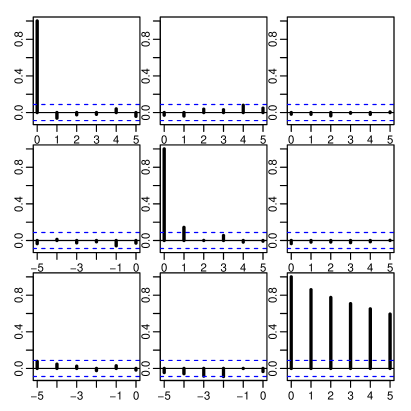
Figure 2: Sample autocorrelation function and realization of the third component of process $(\ref{example.flip})$, based on $n=500$

3 Statistical results

In this section we focus on the estimation of model (3). As seen in the example in Section 2, the autocovariance function is not helpful to identify such models. Note further that even if $\mathbf{Ad}$ is Markovian, an NAR$(1)$ process can generally not be written as a Hidden Markov model (HMM). This is because $\mathbf{X}$ given $\mathbf{Ad}$ is not a sequence of conditionally independent variables and cannot be written as a noisy functional of $Ad_{t-1}$ only, which is required by a HMM, see among others [2] for details on HMM. Consequently, techniques used for HMM cannot be applied here. Instead, the same setting as in Knight et al., [12, 11], Zhu et al., [42] is considered. Thus, the process $\mathbf{X}$ as well as the network $\mathbf{Ad}$ is observed leading to observations $X_{1},\dots,X_{n}$ and $Ad_{1},\dots,Ad_{n-1}$. In such a setting, the consistency of a least square estimate as well as asymptotic normality for model (3) is shown in the first subsection. The results are presented under general assumptions and the asymptotic setting that $d$ is fixed and $n\to\infty$. Later on, we give dependence measure conditions for the underlying dynamic network such that the general assumptions hold. In the second subsection, a simplified version of model (3) is considered. This simplified model is suited for high-dimensional cases, and consequently, the theoretical estimation results are presented nonasymptotically.

3.1 Network autoregressive models

Networks usually come together with some form of sparsity, see among others Section 3.5 in [14]. This means that a vertex has only a connection to a limited number of other vertices and $E\operatorname{sign}(Ad_{1})$ could have some zero entries or might even be a sparse matrix. Thus, $E\operatorname{sign}(G_{j}(Ad_{1})),j=1,\dots,p$ might be sparse matrices as well. That means the number of parameters of model (3) is given by $\sum_{j=1}^{p}\|\operatorname{vec}(E|\operatorname{sign}(G_{j}(Ad_{1}))|)\|_{0}\leq pd^{2}$ and depends on the sparsity of the underlying network. Let $\mathcal{I}{(r)}=\{\tilde{i}=i+(j-1)d,i=1,\dots,d,j=1,\dots,p:1/n\sum_{t=p+1}^{n}e_{r}^{\top}|G_{j}(Ad_{t-j})|e_{i}>0\},r=1,\dots,d$ be a set of indices corresponding to the non-zero coefficients of $\sum_{t=p+1}^{n}|(G_{1}(Ad_{t-1}):\dots:G_{p}(Ad_{t-p}))|$ and $\mathcal{I}{(r)}_{E}=\{\tilde{i}=i+(j-1)d,i=1,\dots,d,j=1,\dots,p:Ee_{r}^{\top}|G_{j}(Ad_{1})|e_{i}>0\},r=1,\dots,d$ is the corresponding population quantity. Note that $\mathcal{I}{(r)}\subseteq\mathcal{I}{(r)}_{E}$ for all $t$. Only parameters corresponding to indices of the set $\mathcal{I}{(r)}_{E}$ are well defined in the sense that they have an influence on the process. We set the other parameters, meaning those corresponding to indices of the set $(\mathcal{I}{(r)}_{E})^{C}$, to zero. Recall that $I_{d;-I}\in\mathds{R}^{(d-|I|)\times d}$ denotes a $d$-dimensional identity matrix without rows $i\in I$ and $I_{d;I}=I_{d;-I^{C}}.$ Let for $r=1,\dots,d,$ $w_{r}=I_{dp;\mathcal{I}{(r)}}(e_{r}^{\top}A_{1},\dots,e_{r}^{\top}A_{p})^{\top}$ and

$$Y_{t-1}^{(r)}=I_{dp;\mathcal{I}{(r)}}((e_{r}^{\top}G_{1}(Ad_{t-1}))\odot X_{t-1},\dots,(e_{r}^{\top}G_{p}(Ad_{t-p}))\odot X_{t-p})^{\top}.$$

Then for $t=p+1,\dots,n$ and $r=1,\dots,d,$ we can write (3) as

$$X_{t;r}=w_{r}^{\top}Y_{t-1}^{(r)}+\varepsilon_{t;r}.$$ (9)

Thus, $w_{r}$ and $\mu_{r}=E\varepsilon_{t;r}$ can be estimated by using the following least square approach given by ${\operatorname{argmin}}_{\hat{w}_{r},\hat{\mu}_{r}}\sum_{t=p+1}^{n}(X_{t;r}-\hat{w}_{r}^{\top}Y_{t_{1}}-\hat{\mu}_{r})^{2}.$ For component $r$, this leads to the following linear system:

$$\begin{pmatrix}\sum_{t=p+1}^{n}X_{t;r}Y^{(r)}_{t-1}-\frac{1}{n-p}\sum_{t_{1},t_{2}=p+1}^{n}Y^{(r)}_{t_{1}-1}X_{t_{2};r}\\ \sum_{t=p+1}^{n}X_{t;r}\end{pmatrix}=$$

$$\begin{pmatrix}0&\sum_{t=p}^{n-1}Y^{(r)}_{t}(Y^{(r)}_{t})^{\top}-\frac{1}{n-p}\sum_{t_{1},t_{2}=p}^{n-1}(Y^{(r)}_{t_{1}})(Y^{(r)}_{t_{2}})^{\top}\\ n-p&\sum_{t=p}^{n-1}(Y^{(r)}_{t})^{\top}\end{pmatrix}\begin{pmatrix}\hat{\mu}_{r}\\ \hat{w}_{r}\end{pmatrix}.$$ (10)

We show the consistency of the least square estimators under general assumptions. Later on, we specify a dependence concept for the underlying network which ensures these general assumptions, see Lemma 3.2.

Assumption 2.

For all $r=1,\dots,d,$ we have, as $n\to\infty$,

1. $EY_{1}^{(r)}=\mu_{Y^{(r)}}$, $1/n\sum_{s=1}^{n}Y^{(r)}_{s}=\mu_{Y^{(r)}}+O_{P}(1/\sqrt{n}),$ and $\Gamma_{Y^{(r)}}(0)=\mbox{Var}(Y_{1}^{r})$, $\|\Gamma_{Y^{(r)}}(0)\|_{2}$, $\|\Gamma_{Y^{(r)}}(0)^{-1}\|_{2}<\infty,$

   $$\frac{1}{n}\sum_{t=1}^{n}(Y^{(r)}_{t}-\mu_{Y^{(r)}})(Y^{(r)}_{t}-\mu_{Y^{(r)}})^{\top}=\mbox{Var}(Y^{(r)}_{1})+O_{P}(1/\sqrt{n}).$$

2. $$\frac{1}{n}\sum_{t=1}^{n}\varepsilon_{t;r}=\mu_{r}+O_{P}(1/\sqrt{n}),$$

   and

   $$\frac{1}{n}\sum_{t=1}^{n}(Y^{(r)}_{t}-\mu_{Y^{(r)}})(\varepsilon_{t+1;r}-\mu_{r})=\mbox{Cov}(Y^{(r)}_{0},\varepsilon_{1})+O_{P}(1/\sqrt{n})=O_{P}(1/\sqrt{n}).$$

3. For all $s=1,\dots,d,E|Y^{(r)}_{0;s}|^{4}<\infty$ and $E|\varepsilon_{0;s}|^{4}<\infty$.

Assumption 3.

For all $r=1,\dots,d,$ we have, as $n\to\infty$,

$$\frac{1}{\sqrt{n}}\sum_{t=1}^{n}(\varepsilon_{t;r}-\mu_{r})(Y^{(r)}_{t-1}-\mu_{Y^{(r)}})^{\top}\overset{D}{\to}\mathcal{N}(0,\Sigma_{\varepsilon}),$$

where $\Sigma_{\varepsilon}=\mbox{Var}(\varepsilon_{0;r})\Gamma_{Y^{(r)}}(0)=\Sigma_{\varepsilon;rr}\Gamma_{Y^{(r)}}(0)$.

Theorem 3.1.

Under Assumption 2 we have for $r=1,\dots,d,$ $\hat{\mu}_{r}=\mu_{r}+O_{P}(1/\sqrt{n}),\hat{w}_{r}=w_{r}+O_{P}(1/\sqrt{n})$. If additionally Assumption 3 holds, we have, as $n\to\infty$,

$$\sqrt{n}\begin{pmatrix}\hat{\mu}_{r}-\mu_{r}\\ \hat{w}_{r}-w_{r}\end{pmatrix}\overset{D}{\to}\mathcal{N}\left(0,\Sigma_{\varepsilon;rr}\begin{pmatrix}1+\mu_{Y^{(r)}}^{\top}\Gamma_{Y^{(r)}}(0)^{-1}\mu_{Y^{(r)}}&0\\ 0&\Gamma_{Y^{(r)}}(0)^{-1}\end{pmatrix}\right).$$

Furthermore, we have for $r,s=1,\dots,p,$ as $n\to\infty$,

$$n\mbox{Cov}(\mu_{r},\mu_{s})\to\Sigma_{\varepsilon;rs}(1+\mu_{Y^{(r)}}^{\top}\Gamma_{Y^{(r)}}(0)^{-1}\mbox{Cov}(Y^{(r)}_{1},Y_{1}^{(s)})\Gamma_{Y^{(s)}}(0)^{-1}\mu_{Y^{(s)}}),$$

$$n\mbox{Cov}(w_{r},w_{s})\to\Sigma_{\varepsilon;rs}\Gamma_{Y^{(r)}}(0)^{-1}\mbox{Cov}(Y^{(r)}_{1},Y_{1}^{(s)})\Gamma_{Y^{(s)}}(0)^{-1}$$

and $n\mbox{Cov}(w_{r},\mu_{s})\to 0.$

The results of Theorem 3.1 can be used to forecast the process $\mathbf{X}$. If $Ad_{n}$ is observed, then let $Y_{n}^{(r)}=I_{dp;\mathcal{I}{(r)}}((e_{r}^{\top}G_{1}(Ad_{n}))\odot X_{n},\dots,(e_{r}^{\top}G_{p}(Ad_{n-p+1}))\odot X_{n-p+1})^{\top}$ and a one-step ahead forecast of $X_{n+1}$ is given by ${\hat{X}}^{(1)}_{n+1;r}=\hat{w}_{r}Y_{n}^{(r)}+\hat{\mu}_{r},r=1,\dots,d.$ Since $\{\varepsilon_{t}\}$ is i.i.d. and $\hat{w}_{r},\hat{\mu}_{r}$ are $\sqrt{n}$ consistent, we have $E(X_{n+1;r}-\hat{X}^{(1)}_{n+1:r})^{2}=e_{r}^{\top}\Sigma_{\varepsilon}e_{r}+O(1/\sqrt{n})$. If $Ad_{n}$ is not observed, $Ad_{n}$ itself needs to be predicted first. This could be done by fitting a dynamic network model to $Ad_{1},\dots,Ad_{n-1}$ and using this model to predict $Ad_{n}$. An $h$-step ahead forecast can be done recursively, which means performing a one-step ahead forecast based on the observations and the results of the $h-1,\dots,1$-step ahead forecasts.

Assumption 2 mainly requires a $\sqrt{n}$ conversion rate of the first and second sample moments of $\mathbf{X}$. An absolutely summable autocovariance function of $\mathbf{X}$ is sufficient for the convergence of the first sample moments. As pointed out in Lemma 2.2 and Lemma 2.3, the autocovariance of $\mathbf{X}$ depends on the dependency structure of $\mathbf{Ad}$. For simplicity, consider the following network moving average process $X_{t}=Ad_{t-1}\varepsilon_{t-1}+\varepsilon_{t},E\varepsilon_{1}=\mu,\mbox{Var}\varepsilon_{1}=\Sigma_{\varepsilon}$ where $\mathbf{Ad}$ and $\{\varepsilon_{t}\}$ are independent. Following Lemma 2.3, we obtain $\sum_{h=0}^{\infty}\Gamma_{X}(h)=(\Sigma_{\varepsilon}+E(Ad_{1}\Sigma_{\varepsilon}Ad_{1}^{\top})+(EAd_{1}\Sigma_{\varepsilon})+\sum_{h=0}^{\infty}\mbox{Cov}(Ad_{h}\mu,Ad_{0}\mu)$. Hence, even for this simple moving average process, a summmable autocovariance function can be obtained only if $\mathbf{Ad}$ possesses some sort of short-range dependence. Several general dependency concepts exists which could describe a short-range dependency structure such as mixing[3], some weak dependency concepts[7] or physical dependence[33, 35, 37, 17]. Since the concept of physical dependence works well also in the high-dimensional case, see among others [40, 41], this concept is used to quantify the dependence structure of $\mathbf{Ad}$.

To elaborate, let $\{\xi_{t}\}$ be a sequence of i.i.d. random vectors of dimension $\tilde{d}$ such that $\{\Xi_{t}=(\varepsilon_{t},\xi_{t})\}$ is also an i.i.d. sequence. Furthermore, let $Ad_{t}=H(\Xi_{t},\Xi_{t-1},\dots)$, where $H$ is some measurable function to $[-1,1]^{d\times d}$. Denote by $\Xi_{t}^{\prime}$ an i.i.d. copy of $\Xi_{t}$ and let for some $q>0$ $\delta_{q}(\mathbf{Ad},j)=\max_{r,i=1,\dots,d}\linebreak\|e_{r}^{\top}(Ad_{j}-Ad_{j}^{*})e_{i}\|_{E,q},$ where $Ad_{j}^{*}=H(\Xi_{j},\Xi_{j-1},\dots,\Xi_{1},\Xi_{0}^{\prime},\Xi_{-1},\Xi_{-2},\dots)$ is a coupled version of $Ad_{j}$ with $\Xi_{0}$ in the latter being replaced by $\Xi_{0}^{\prime}$. Since $H$ is a function to $[-1,1]^{d\times d}$, $\delta_{q}(\mathbf{Ad},j)<\infty$ for $q\geq 1$. Furthermore, let $\Delta_{q}(\mathbf{Ad})=\sum_{j=0}^{\infty}\delta_{q}(\mathbf{Ad},j).$ The process $\mathbf{Ad}$ is denoted as $q$-stable if $\Delta_{q}(\mathbf{Ad})<\infty$. This property still holds for some nonlinear transformations, see [33, 34]. E.g. consider a polynomial transformation given by $\{g(Ad_{t})=Ad_{t}^{k}\}$. Note that for some matrices $A,B$ we have $A^{k}-B^{k}=\sum_{s=0}^{k-1}A^{s}(A-B)B^{j-1-s}$. If $\|\mathbf{Ad}\|_{\infty}\leq C$, then $\delta_{q/2}(\{g(Ad_{t})\},j)=\delta_{q}(\mathbf{Ad},j)C^{k-1}k$. Without assuming any sparsity, an upper bound is given by $C\leq d$. This dependency concept covers a wide range of processes among them many nonlinear time series, see [33, 35, 37] for examples. Furthermore, this concept includes nonlinear Markov chains, meaning $\mathbf{Ad}$ can be given by $Ad_{t}=H(Ad_{t-1},\Xi_{t})$. Zhang et al., [41] pointed out that a stable process is obtained if $H$ possesses some form of Lipschitz-continuity. Then, $\delta_{q}(\mathbf{Ad},j)=O(\rho^{j})$ for some $\rho\in(0,1)$, see Example 2.4 in [41] or Example 2.1 in [5] for details. A stable vector autoregressive process possesses also such geometrically decaying physical dependence coefficients, see among others Example 2.2 in [5]. Note that many dynamic network models, e.g. Temporal ERGMs [9], are Markovian.

Lemma 3.2.

If Assumption 1a) holds, $\mathbf{Ad}_{G}=\{\widetilde{G(Ad}_{t})\}$ is $2q$-stable, and $\max_{r}\|\varepsilon_{0;r}\|_{E,2q}<\infty$ for some $q\geq 1$, then $\mathbf{X}$ is $q$-stable. If the above conditions hold for $q\geq 4$, then Assumption 2 and 3 hold.

3.2 Network autoregressive models for large dimension

The number of parameters in model (3) is of size $O(pd^{2})$. If the underlying network is not very sparse, a reasonable estimate could be only obtained if $d\ll n$. Hence, in order to handle high-dimensional cases, meaning $d$ is of the same order as $n$ or even larger, we follow Knight et al., [11] and simplify model (3). For each component, the influence of the own lagged components is modeled separately, thus, we set $e_{s}^{\top}G_{j}(\cdot)e_{s}=0$ for all $s=1,\dots,d,j=1,\dots,p$. Then, the simplified model is given by

$$X_{t;r}=\sum_{j=1}^{p}\alpha_{j,r}X_{t-j;r}+\beta_{j,r}e_{r}^{\top}G_{j}(Ad_{t-j})X_{t-j}+\varepsilon_{t;r},r=1,\dots,p,$$ (11)

where $\alpha_{j,r},\beta_{j,r}\in\mathds{R},j=1,\dots,p,r=1,\dots,d$ and $E\varepsilon_{t;r}=\mu_{r}$. Hence, this simplified model possesses in total only $d(2p+1)$ parameters or more precisely only $2p+1$ parameters for each component of the time series independently of the dimension. The parameter $\alpha$ quantifies the linear influence of the same component and $\beta$ the linear influence of the other components. Note that model (11) can be written as

$$X_{t}=\sum_{j=1}^{p}\begin{pmatrix}\alpha_{j,1}&\beta_{j,1}&\dots&\beta_{j,1}&\beta_{j,1}\\ \beta_{j,2}&\alpha_{j,2}&\beta_{j,2}&\dots&\beta_{j,2}\\ \vdots&\ddots&\ddots&\ddots&\vdots\\ \beta_{j,d-1}&\dots&\beta_{j,d-1}&\alpha_{j,d-1}&\beta_{j,d-1}\\ \beta_{j,d}&\dots&\beta_{j,d}&\beta_{j,d}&\alpha_{j,d}\end{pmatrix}\odot(I_{p}+G_{j}(Ad_{t-j}))X_{t-j}+\varepsilon_{t},$$ (12)

and consequently fits into the framework (3). We denote the process as Large Network AutoRegression (LNAR) and the coefficient matrices occurring in (12) by $A_{j,\alpha,\beta},j=1,\dots,p$. Since a LNAR is an NAR process, a stationary solution is given by Lemma 2.2 if $\det(I-\sum_{j=1}^{p}|A_{j,\alpha,\beta}|z^{j})\not=0$ for all $|z|\leq 1$ or $\rho(\tilde{A}\odot\tilde{G}(\cdot))<1$. If no restrictions on the underlying network are imposed, then the first condition implies that in order to obtain a stationary solution, the parameter space depends on $d$. This is not the case we would like to consider here, which is why conditions on the underlying network are imposed. We require that $\|G_{j}(\cdot)\|_{\infty}\leq 1,j=1,\dots,p$, which means that the sum of weights of the edges going into a vertex does not grow with the dimension $d$. To simplify notation, we bound the sum of weights by $1$. Knight et al., [11] require a similar condition in the case of a static network. Under this condition, we obtain a stationary solution if $\max_{r=1,\dots,p}\sum_{j=1}^{p}|\alpha_{j,r}|+|\beta_{j,r}|\leq C_{\lambda}<1$, see the following Lemma 3.3. Note that under the same conditions Knight et al., [11] obtain a stationary solution in the case of a static network.

Lemma 3.3.

If $\|G_{j}(\cdot)\|_{\infty}\leq 1$ for $j=1,\dots,p,$ and $\max_{r=1,\dots,p}\sum_{j=1}^{p}|\alpha_{j,r}|+|\beta_{j,r}|\leq C_{\lambda}<1$, then (11) fulfills Assumption 1b) and possesses a stationary solution. The solution takes the form

$$X_{t}=\sum_{j=0}^{\infty}(e_{1}\otimes I_{d})^{\top}\prod_{s=1}^{j}(\tilde{A}_{\alpha,\beta}\odot G(\widetilde{Ad}_{t-s}))(e_{1}\otimes I_{d})\varepsilon_{t-j}=:\sum_{j=0}^{\infty}B_{t,j}\varepsilon_{t-j},$$ (13)

where

$$\widetilde{G(Ad)}_{t-1})=$$

$$\begin{pmatrix}I_{d}+G_{1}(Ad_{t-1})&I_{d}+G_{2}(Ad_{t-2})&\dots&I_{d}+G_{p-1}(Ad_{t-p+1})&I_{d}+G_{p}(Ad_{t-p})\\ I_{d}&0&\dots&0&0\\ 0&I_{d}&&0&0\\ \vdots&&\ddots&\vdots&\vdots\\ 0&0&\dots&I_{d}&0\end{pmatrix}.$$

Furthermore, $\rho(|\tilde{A}_{\alpha,\beta}\odot\tilde{G}(\cdot)|)\leq C_{\lambda}^{1/p}.$

For component $r=1,\dots,d$, let $w_{r}=(\alpha_{1,r},\beta_{1,r},\dots,\alpha_{p,r},\beta_{p,r})^{\top}\in\mathds{R}^{2p}$ and $Y_{t-1}^{(r)}=(X_{t-1;r},e_{r}^{\top}G_{1}(Ad_{t-1})X_{t-1},\dots,X_{t-p;r},e_{r}^{\top}G_{p}(Ad_{t-p})X_{t-p})^{\top}$. Then, (11) can be written as $X_{t;r}=w_{t}^{\top}Y_{t-1}^{(r)}+\varepsilon_{t;r}$. This is the same framework as in Section 3.1, and the linear system (3.1) gives a least square estimate. To cover a high-dimensional setting, we study the theoretical properties of this estimator in a nonasymptotic framework as it is done in the high-dimensional vector autoregressive case, see among others [1]. We make use of the Nagaev inequality for dependent variables, see Theorem 2 in [18], to formulate nonasymptotic error bounds. Again, the physical dependency concept is used to quantify the dependency structure of $\mathbf{Ad}$, see the following Assumption 4.

Assumption 4.

For $j=1,\dots,p$ let $\|G_{j}(\cdot)\|_{\infty}\leq 1$ and let $\mathbf{Ad}_{G\mathds{1}}=\{\max_{j=1,\dots,p}\linebreak\max_{r}e_{r}^{\top}|G_{j}(Ad_{t})|\mathds{1},t\in\mathds{Z}\}$ be $2q$-stable with $\sum_{k=1}^{\infty}k\delta_{2q}(\mathbf{Ad}_{G\mathds{1}},k)\leq C_{G}$, where $C_{G}<\infty$ is some constant. Furthermore, let $\max_{r=1,\dots,d}\sum_{j=1}^{p}|\alpha_{j,r}|+|\beta_{j,r}|\leq C_{\lambda}^{p}<1$ and $\||\tilde{A}_{\alpha,\beta}\odot\tilde{G}(\cdot)|^{j}\|_{\infty}\leq C_{A}C_{\lambda}^{j}$. The constants appearing here do not depend on the dimension $d$.

Note that $\|G(\cdot)\|_{\infty}\leq 1$ and $\max_{r=1,\dots,d}\sum_{j=1}^{p}|\alpha_{j,r}|+|\beta_{j,r}|\leq C_{\lambda}^{p}<1$ implies $\||\tilde{A}_{\alpha,\beta}\odot\tilde{G}(\cdot)|^{j}\|_{\infty}\leq\||\tilde{A}_{\alpha,\beta}\odot\tilde{W}|\|_{\infty}^{j}\leq 1$. Furthermore, we have a bound for the largest eigenvalue $\rho(|\tilde{A}_{\alpha,\beta}\odot\tilde{W}|)\leq C_{\lambda}<1$, see the proof of Lemma 3.3. If $G_{j}(\cdot)=W_{j}\odot\cdot,$ where $W_{j}\in[-1,1]^{d\times d}$ and $\|W_{j}\|_{\infty}\leq 1$ for all $j$, then $\delta_{2q}(\mathbf{Ad}_{G\mathds{1}},k)=\|\max_{r}\max_{j}e_{r}^{\top}(G_{j}(Ad_{k})-G_{j}(Ad_{k}^{*}))\mathds{1}\|_{E,2q}=\|\max_{r}\max_{j}e_{r}^{\top}(W_{j}\odot(Ad_{k}-Ad_{k}^{*}))\mathds{1}\|_{E,2q}\leq\max_{j}\|W_{j}\|_{\infty}\delta(\mathbf{Ad},k)\leq\delta(\mathbf{Ad},k)$. If $\mathbf{Ad}_{G\mathds{1}}$ possesses geometrically decaying physical dependence coefficients, then $\sum_{k=1}^{\infty}k\delta_{2q}(\mathbf{Ad}_{G\mathds{1}},k)\leq C_{G}<\infty$.

This Assumption implies that $\mathbf{X}$ as well as $\{Y_{t}^{(r)},t\in\mathds{Z}\}$ are $q$-stable and their physical dependency quantity $\sum_{j=0}^{\infty}\delta_{q}(\cdot,j)$ can be bounded independently from the dimension $d$, see Lemma 3.4 for details.

Lemma 3.4.

If Assumption 4 holds, and $\max_{i}\|\varepsilon_{0,i}\|_{E,2q}<\infty$, then $\mathbf{X}$ generated by model (11) is $q$-stable and $\sum_{j=0}^{\infty}\delta_{q}(\{\max_{r=1,\dots,d}X_{t;r},t\in\mathds{Z}\},j)\leq\max_{i}\|\varepsilon_{0,i}\|_{E,2q}C_{A}/(1-C_{\lambda})(C_{A}/C_{\lambda}/(1-C_{\lambda})\sum_{j=0}^{\infty}\delta_{2q}(\mathbf{Ad}_{G\mathds{1}},j)+1)$. Furthermore, we have for $k=1,\dots,2p$, $\sum_{j=0}^{\infty}j\delta_{q}(\{\max_{r}e_{k}^{\top}Y_{t}^{(r)},t\in Z\},j)\leq C_{\delta_{Y}},$ where

$$C_{\delta Y}=\max_{i}\|\varepsilon_{0,i}\|_{E,2q}\frac{C_{A}}{1-C_{\lambda}}\Big{[}\frac{C_{\lambda}}{1-C_{\lambda}}+C_{G}(1+\frac{C_{A}(2-C_{\lambda})}{(1-C_{\lambda})^{2}})\Big{]}.$$

With this results, we can formulate the nonasymptotic error bounds. In order to handle a high-dimensional setting an import result is to obtain an error bound which grows only moderately with $d$, the dimension of the process. Note that in contrast to the estimation of a high-dimensional VAR system, e.g. [13], the dimension of the parameter vector does not depend on $d$. This enables us to obtain an error bound which does not depend on $d$ at all, see the following Theorem 3.5 for details.

Theorem 3.5.

Under Assumption 4 we have for component $r=1,\dots,d,$ of model (11), and the estimators given by the linear system (3.1) for some $y\in\mathds{R}$ with probability of at least $(1-c_{q}(n-p)^{1-q}y^{-q}-(c_{q}^{\prime}+2)\exp(-c_{q}(n-p)y^{2}))^{4}=:C_{q}(n,y)^{4}$, where $c_{q},c_{q}^{\prime}$ are constants depending on $q$ only, the following error bounds

$$\|\hat{w}_{r}-w_{r}\|_{1}\leq y\frac{\sqrt{2p}C_{\delta Y}(\|\varepsilon_{0;r}\|_{E,q}+C_{\delta Y}y+\mu_{r}+\|\mu_{Y^{(r)}}\|_{1})}{\rho(\Gamma^{-1})-y2pC_{\delta Y}(2C_{A}/(1-C_{\lambda})+2\|\mu_{Y^{(r)}}\|_{1}+yC_{\delta Y})},$$ (14)

$$|\hat{\mu}_{r}-\mu_{r}|\leq (\|\mu_{Y^{(r)}}\|_{1}+yC_{\delta Y})\|\hat{w}_{r}-w_{r}\|_{1}+yC_{\delta Y}.$$ (15)

For $y=o(1/\sqrt{n})$, the error tends to zero but the probability still faces $1$ with increasing $n$. This rate is independent of the dimension $d$. This enables us to use LNAR for forecasting in a high-dimensional framework. The forecasting procedure is analogue to the one for the NAR approach, see the end of the previous subsection.

4 Numerical Examples

In this section, the forecasting performance of the models presented in Section 2 is investigated in finite samples. For a low-dimensional example and a high-dimensional example, we forecast $X_{n+1},\dots,X_{n+h}$ based on observations $X_{1},\dots,X_{n}$ and $Ad_{1},\dots,Ad_{n-1}$, where $h=4$. The performance is measured by computing the mean squared error (MSE) averaged over all components via a Monte Carlo simulation using $B=1000$ repetitions, meaning

$$MSE(\hat{X}_{n+h}^{(h)})\approx 1/d\sum_{j=1}^{d}1/B\sum_{i=1}^{B}(X_{n+h,i;j}-\hat{X}_{n+h,i;j}^{(h)})^{2},$$

where $X_{n,i;j}$ denotes the $j$th component of the $n$th observation of the $i$th Monte Carlo sample. In the following, we denote the approach using model (3) as NAR and the approach using model (11) as LNAR. As a benchmark, we use a vector autoregressive model given by $X_{t}=\sum_{j=1}^{p}A_{j}X_{t-j}+\varepsilon_{t}$, where $A_{1},\dots,A_{p}\in\mathds{R}^{d\times d}$. This approach is denoted by VAR. The three models considered have a tuning parameter $p$ which specifies the lag order. For all three models, the Bayesian Information Criterion (BIC) is used to automatically choose the lag-order $p$, see among others Section 5.5 in [4].

The approaches NAR and LNAR make use of the underlying network structure. That means in order to compute $X_{n+h}^{h}$, the approaches NAR and LNAR require an observation or at least an estimate of the underlying network structure. Both cases are considered here, in the first case we forecast $Ad_{n},\dots,Ad_{n+h-1}$ based on the observations $Ad_{1},\dots,Ad_{n-1}$, and in the second case we assume that $Ad_{n},\dots,Ad_{n+h-1}$ is observed. In order to distinguish between these two cases, we denote the forecast of approach NAR based on an estimated network by NAR$(\widehat{\mathbf{Ad}})$ and the forecast based on a known network structure by NAR$(\mathbf{Ad})$. An analogue notation is used for LNAR.

All computations are done in R [29] using the additional packages tergm, BigVAR, markovchain [16, 26, 30].

In the first example, a network with $4$ vertices is considered. The adjacency matrix process $\mathbf{Ad}$ is a Markovian process and the edges are independent from each other. The process $\mathbf{Ad}$ is given by

$$\left(P(Ad_{t;ij}=1|Ad_{t-1;ij}=1)\right)_{i,j=1,\dots,d} =\begin{pmatrix}0.95&0.70&0.99&0\\ 0&0.95&0.70&0\\ 0.99&0.50&0.95&0.95\\ 0.30&0&0&0.95\end{pmatrix},$$

$$\left(P(Ad_{t;ij}=1|Ad_{t-1;ij}=0)\right)_{i,j=1,\dots,d} =\begin{pmatrix}0.05&0.10&0.01&0\\ 0&0.05&0.30&0\\ 0.01&0.50&0.05&0.05\\ 0.30&0&0&0.05\end{pmatrix}.$$ (16)

The process $\mathbf{X}$ is an NAR$(1)$ process and is given by

$$X_{t}=\left(\alpha\odot Ad_{t-1}\right)X_{t-1}+\varepsilon_{t},t\in\mathds{Z},\varepsilon_{1}\sim\mathcal{N}\left((-1,4,-9,16)^{\top},I_{4}\right),$$ (17)

where $\alpha=\begin{pmatrix}0.25&0.7&0&0\\ 0&0.25&0.7&0\\ 0&0&0.25&0.7\\ 0.7&0&0&0.25\end{pmatrix}$.

[width=loop=TRUE,autoplay=TRUE]1MarkovNetwork_d_4

Figure 3: The upper figure presents a realization of the network of the example given by $(\ref{example.1.network})$ and a realization of the time series $X$ given by $(\ref{example.1.process})$. Red dots indicate the current time point. This figure contains animation only visible on screen. The lower graphic presents the sample autocovariance function of $X$.

A realization of the network, the time series, and the sample autocovariance function are displayed in Figure 3. The edges $(3,1)$ and $(1,3)$ have a coefficient of $0$, hence, whether they are present or not, they do not influence the time series $\mathbf{X}$.

The model structure of $\mathbf{Ad}$ is used to compute a forecast of $\mathbf{Ad}$. Thus, for each component of $\mathbf{Ad}$, a discrete Markov chain is fitted to $Ad_{1},\dots,Ad_{n-1}$, and this Markov chain is then used to obtain a forecast for $Ad_{n},\dots,Ad_{n+h-1}$. For this the R-package markovchain was used.

The mean squared errors for the forecast horizons $h=1,\dots,4$ are displayed in Table 1. Note that an optimal one-step ahead forecast for this process would possess a forecast error of $1$. This can be nearly achieved by NAR with a known network structure and moderate sample size. If the underlying network structure is unknown, NAR outperforms the other approaches for the forecast horizons up to $h=3$. For forecast horizons further ahead, VAR performs slightly better. This drop in performance for horizons further ahead is mainly caused by the estimate of the underlying network structure. The approach used here causes that $\hat{A}d_{n+h}^{(h)}$ is identical for all horizons $h=1,\dots,4$. This estimate gets poorer, the larger $h$ is.

n		$h=1$	$h=2$	$h=3$	$h=4$
	NAR$(\mathbf{Ad})$	1.24	1.42	1.53	1.61
	NAR$(\widehat{\mathbf{Ad}})$	1.47	2.80	3.67	4.14
50	LNAR$(\mathbf{Ad})$	1.89	2.32	2.62	2.91
	LNAR$(\widehat{\mathbf{Ad}})$	2.00	3.18	4.04	4.63
	VAR	2.83	3.56	4.08	4.35
	NAR$(\mathbf{Ad})$	1.07	1.19	1.23	1.25
	NAR$(\widehat{\mathbf{Ad}})$	1.20	2.76	3.56	4.13
100	LNAR$(\mathbf{Ad})$	1.78	2.18	2.35	2.47
	LNAR$(\widehat{\mathbf{Ad}})$	1.83	3.08	3.86	4.49
	VAR	2.65	3.40	3.80	4.08
	NAR$(\mathbf{Ad})$	1.01	1.12	1.14	1.16
	NAR$(\widehat{\mathbf{Ad}})$	1.11	2.63	3.55	4.09
200	LNAR$(\mathbf{Ad})$	1.71	2.04	2.20	2.30
	LNAR$(\widehat{\mathbf{Ad}})$	1.74	2.88	3.71	4.30
	VAR	2.63	3.30	3.69	4.01
	NAR$(\mathbf{Ad})$	1.01	1.11	1.14	1.15
	NAR$(\widehat{\mathbf{Ad}})$	1.13	2.66	3.41	4.10
500	LNAR$(\mathbf{Ad})$	1.69	2.00	2.14	2.23
	LNAR$(\widehat{\mathbf{Ad}})$	1.73	2.91	3.60	4.32
	VAR	2.60	3.27	3.60	3.92

Table 1: Mean squared error averaged over all components for process (17) and the forecast horizons $h=1,\dots,4$.

In the second example, a Separable Temporal Exponential Random Graph Model (STERGM) is considered, see Krivitsky and Handcock, [15] and also [16] for the used R package tergm. The network is generated using simulate.stergm of the R-package tergm with dissolution coefficient $4$, formation coefficient $-\log\Big{(}(d/5-1)(1+\exp(4))-1\Big{)}$, and a mean density of $5/d$. Networks of the sizes $d=10,33,100$, and $500$ are considered, and for each network size the sample sizes $n=100,200$, and $500$. For $d=500$, such a network has about $4000$ edge changes from $t=1$ to $t=100$. Let $Ad_{t}$ be the adjacency matrix of such a network at time $t$ and let $B_{t}=\operatorname{diag}((1/(\mathds{1}^{\top}Ad_{t}e_{i})_{i=1,\dots,d})$ be a diagonal matrix, where $1/0$ is defined as $0$. This defines the function $G(Ad_{t})=Ad_{t}B_{t}$ and let $AdG_{t}=G(Ad_{t})=Ad_{t}^{\top}B_{t}$. This means $e_{i}^{\top}AdG_{t}$ apportions equally the weight $1$ among the in-going edges to vertex $i$ at time $t$, and we have $\|AdG_{t}\|_{\infty}=\max_{i}\sum_{s=1}^{d}Ad_{t;si}/(\sum_{s=1}^{d}Ad_{t;si})\leq 1$. Then, the process $\mathbf{X}$ is given by the following LNAR(1) model

$$X_{t;r}=0.9(r/d)X_{t-1;r}+0.9(d-r)/dAdG_{t-1}X_{t-1}+\varepsilon_{t;r},$$ (18)

where $\varepsilon_{t}\sim\mathcal{N}(\mu,5\Sigma_{\varepsilon})$ and $\mu=(1(-1),2(-1)^{2},3(-1)^{3},\dots,d(-1)^{d})^{\top}$ and $\Sigma_{\varepsilon}$ is a banded matrix with ones on the diagonal and $0.25(-1)^{j+1},j=1,\dots,d-1$ on the first off diagonal. The function $G$ is considered as known, meaning $AdG_{1},\dots,AdG_{n-1}$ is observed.

Two approaches are used to obtain a forecast for $Ad_{n},\dots,Ad_{n+h-1}$. The first approach fits a STERGM model to $Ad_{1},\dots,Ad_{n-1}$ and then generates $\hat{A}d_{n-1+h}^{(h)}$ by simulating the fitted model with $Ad_{n-1}$ as a starting value. This forecast is denoted as $\widehat{Ad}_{1}$. The second approach fits for each component independently a discrete Markov chain and uses this to forecast $\mathbf{Ad}$. The second approach is denoted as $\widehat{Ad}_{2}$.

Since a standard VAR model cannot be applied well to a high-dimensional setting, the VAR estimation is modified by adding sparsity constraints, meaning a coefficient $A_{j,rc}$ is set to zero for $j=1,\dots,p$ if $\sum_{t=1}^{n}e_{r}^{\top}AdG_{t}e_{c}=0$. This is motivated by the fact that in model (18) if $Ee_{r}^{\top}AdG_{t}e_{c}=0$, then $X_{t-j;c},j=1,\dots,p$ do not directly influence $X_{t;r}$. Furthermore, forecasts given by the R-package BigVAR are included as additional benchmarks, see [26]. There the idea is that the underlying VAR model is sparse but the sparsity structure is unknown. It can be estimated by using a LASSO approach, see among others [1, 13]. The forecast obtained by a such a model of order $p$ is denoted by BigVAR$(p)$, where $p=1,2$.

The mean squared errors of the forecasts are displayed in Table 3 to Table 4. Note that an optimal one-step ahead forecast would possess a forecast error of $5$. With a known network structure at hand, LNAR is nearly able to achieve such optimal results independently of the dimension. Is the future network unknown, then the forecasting performance of NAR and LNAR drop considerably. Especially for LNAR, the loss of performance due to an unknown network structure seems to increase with the dimension of the process. Of the two approaches used to forecast the network, a better performance is given by the network forecasting approach $\widehat{Ad}_{1}$ for NAR as well as LNAR. Given the network forecast $\widehat{Ad}_{1}$, both approaches still outperform all others namely VAR and BigVAR$(p),p=1,2$. As mentioned, VAR uses the underlying network structure to set sparsity constraints such that the number of parameters can be reduced. In all settings considered, VAR outperforms BigVAR$(p),p=1,2$. This indicates that for this process the network induced sparsity constraints are more helpful than a free but unknown sparsity setting as given in BigVAR. However, note that the amount of parameters which are estimated for the approaches NAR and VAR depend on the set $\mathcal{I}_{n}:=\{i,r=1,\dots,d:1/n\sum_{t=1}^{n-1}e_{r}^{\top}|Ad_{t}|e_{i}>0\},$ and we have $|\mathcal{I}_{n}|\leq|\mathcal{I}_{m}|$ for $m\geq n$. This could explain why these two approaches do not gain immediately from an increasing sample size for larger dimensions.

In order to get a better overview of the results, we set the MSE of the approach VAR as basing point, meaning all MSE values are divided by the corresponding VAR’s MSE. An average over all sample sizes and forecast horizons leads to Table 2. These aggregated results support the argument that the approaches NAR and LNAR benefit from the underlying network structure and even when the future network structure is unknown and needs to be estimated itself, there is still a benefit. For higher dimensions, only LNAR performs well whereas the performance of all others drop dramatically, meaning that the network induced sparsity does not seem to be sufficient to obtain good estimation results in this setting.

$d$	10	33	100	500
NAR$(\mathbf{Ad})$	0.35	0.33	0.44	0.51
NAR$(\widehat{\mathbf{Ad}}_{1})$	0.71	0.74	0.78	0.77
NAR$(\widehat{\mathbf{Ad}}_{2})$	0.84	0.93	0.95	0.96
LNAR$(\mathbf{Ad})$	0.27	0.04	0.01	$<0.01$
LNAR$(\widehat{\mathbf{Ad}}_{1})$	0.66	0.60	0.56	0.53
LNAR$(\widehat{\mathbf{Ad}}_{2})$	0.80	0.85	0.81	0.80
VAR	1.00	1.00	1.00	1.00
BigVAR$(1)$	2.99	5.35	6.35	7.88
BigVAR$(2)$	3.24	5.71	6.68	8.09

Table 2: Relative mean squared error (basing point: VAR) for process (18) averaged over forecast horizons and sample sizes.

		$d=10$				$d=33$
$n$	Model	$h=1$	$h=2$	$h=3$	$h=4$	$h=1$	$h=2$	$h=3$	$h=4$
	NAR$(\mathbf{Ad})$	6.9E+00	1.1E+01	1.5E+01	1.9E+01	3.4E+01	7.2E+01	1.1E+02	1.6E+02
	NAR$(\widehat{\mathbf{Ad}}_{1})$	9.7E+00	1.8E+01	2.7E+01	3.6E+01	5.6E+01	1.3E+02	2.1E+02	2.9E+02
	NAR$(\widehat{\mathbf{Ad}}_{2})$	1.2E+01	2.3E+01	3.2E+01	4.3E+01	7.5E+01	1.6E+02	2.5E+02	3.4E+02
	LNAR$(\mathbf{Ad})$	5.1E+00	7.1E+00	8.5E+00	9.6E+00	5.3E+00	7.2E+00	8.5E+00	9.4E+00
100	LNAR$(\widehat{\mathbf{Ad}}_{1})$	8.3E+00	1.6E+01	2.3E+01	3.1E+01	4.1E+01	1.0E+02	1.7E+02	2.4E+02
	LNAR$(\widehat{\mathbf{Ad}}_{2})$	1.1E+01	2.1E+01	2.9E+01	3.8E+01	6.7E+01	1.5E+02	2.3E+02	3.1E+02
	VAR	1.3E+01	2.7E+01	4.1E+01	5.5E+01	6.9E+01	1.8E+02	3.2E+02	4.9E+02
	BigVAR$(1)$	4.4E+01	6.8E+01	8.8E+01	1.0E+02	5.4E+02	7.3E+02	8.9E+02	1.0E+03
	BigVAR$(2)$	4.8E+01	7.2E+01	9.1E+01	1.1E+02	5.7E+02	7.6E+02	9.2E+02	1.0E+03
	NAR$(\mathbf{Ad})$	5.9E+00	8.8E+00	1.1E+01	1.3E+01	2.9E+01	5.7E+01	8.5E+01	1.1E+02
	NAR$(\widehat{\mathbf{Ad}}_{1})$	9.4E+00	1.8E+01	2.8E+01	3.7E+01	5.7E+01	1.2E+02	1.9E+02	2.6E+02
	NAR$(\widehat{\mathbf{Ad}}_{2})$	1.1E+01	2.2E+01	3.2E+01	4.2E+01	7.6E+01	1.5E+02	2.4E+02	3.2E+02
	LNAR$(\mathbf{Ad})$	5.2E+00	7.2E+00	8.3E+00	9.2E+00	5.1E+00	6.9E+00	8.0E+00	8.7E+00
200	LNAR$(\widehat{\mathbf{Ad}}_{1})$	8.9E+00	1.7E+01	2.6E+01	3.5E+01	4.2E+01	9.3E+01	1.5E+02	2.2E+02
	LNAR$(\widehat{\mathbf{Ad}}_{2})$	1.1E+01	2.1E+01	3.0E+01	4.0E+01	6.6E+01	1.4E+02	2.2E+02	3.0E+02
	VAR	1.3E+01	2.6E+01	4.0E+01	5.3E+01	6.2E+01	1.5E+02	2.7E+02	4.1E+02
	BigVAR$(1)$	5.2E+01	8.1E+01	1.0E+02	1.2E+02	6.9E+02	9.3E+02	1.1E+03	1.2E+03
	BigVAR$(2)$	6.0E+01	9.0E+01	1.1E+02	1.3E+02	7.5E+02	9.8E+02	1.2E+03	1.3E+03
	NAR$(\mathbf{Ad})$	5.1E+00	7.3E+00	8.8E+00	9.9E+00	1.9E+01	3.6E+01	5.2E+01	6.5E+01
	NAR$(\widehat{\mathbf{Ad}}_{1})$	9.1E+00	1.7E+01	2.6E+01	3.3E+01	4.9E+01	1.1E+02	1.8E+02	2.5E+02
	NAR$(\widehat{\mathbf{Ad}}_{2})$	1.1E+01	2.0E+01	2.9E+01	3.8E+01	6.5E+01	1.4E+02	2.2E+02	3.0E+02
	LNAR$(\mathbf{Ad})$	5.0E+00	7.0E+00	8.3E+00	9.2E+00	5.0E+00	6.7E+00	7.8E+00	8.4E+00
500	LNAR$(\widehat{\mathbf{Ad}}_{1})$	9.0E+00	1.7E+01	2.6E+01	3.3E+01	3.9E+01	9.5E+01	1.6E+02	2.3E+02
	LNAR$(\widehat{\mathbf{Ad}}_{2})$	1.1E+01	2.0E+01	2.9E+01	3.7E+01	5.7E+01	1.3E+02	2.1E+02	2.9E+02
	VAR	1.2E+01	2.3E+01	3.5E+01	4.5E+01	5.4E+01	1.4E+02	2.5E+02	3.6E+02
	BigVAR$(1)$	5.0E+01	8.6E+01	1.1E+02	1.3E+02	5.1E+02	8.6E+02	1.1E+03	1.3E+03
	BigVAR$(2)$	5.6E+01	9.2E+01	1.2E+02	1.3E+02	5.7E+02	9.2E+02	1.2E+03	1.3E+03

Table 3: Mean squared error for process (18) with dimension $d=10,33$ and the forecast horizons $h=1,\dots,4$.

		$d=100$				$d=500$
$n$	Model	$h=1$	$h=2$	$h=3$	$h=4$	$h=1$	$h=2$	$h=3$	$h=4$
	NAR$(\mathbf{Ad})$	2.6E+02	5.7E+02	9.5E+02	1.4E+03	5.5E+03	1.2E+04	2.0E+04	2.7E+04
	NAR$(\widehat{\mathbf{Ad}}_{1})$	4.2E+02	9.5E+02	1.5E+03	2.1E+03	9.5E+03	2.3E+04	3.7E+04	5.1E+04
	NAR$(\widehat{\mathbf{Ad}}_{2})$	5.7E+02	1.2E+03	1.8E+03	2.5E+03	1.4E+04	3.0E+04	4.6E+04	6.1E+04
	LNAR$(\mathbf{Ad})$	5.2E+00	7.3E+00	8.4E+00	9.3E+00	5.3E+00	7.2E+00	8.3E+00	9.1E+00
100	LNAR$(\widehat{\mathbf{Ad}}_{1})$	2.8E+02	7.3E+02	1.2E+03	1.8E+03	6.9E+03	1.8E+04	3.1E+04	4.4E+04
	LNAR$(\widehat{\mathbf{Ad}}_{2})$	4.8E+02	1.1E+03	1.7E+03	2.4E+03	1.2E+04	2.8E+04	4.3E+04	5.9E+04
	VAR	4.8E+02	1.4E+03	2.6E+03	4.3E+03	1.2E+04	3.5E+04	7.0E+04	1.2E+05
	BigVAR$(1)$	5.1E+03	6.4E+03	7.3E+03	8.1E+03	1.7E+05	1.9E+05	2.1E+05	2.2E+05
	BigVAR$(2)$	5.3E+03	6.4E+03	7.4E+03	8.2E+03	1.7E+05	1.9E+05	2.1E+05	2.2E+05
	NAR$(\mathbf{Ad})$	3.1E+02	6.5E+02	9.7E+02	1.3E+03	6.6E+03	1.5E+04	2.5E+04	3.7E+04
	NAR$(\widehat{\mathbf{Ad}}_{1})$	5.0E+02	1.1E+03	1.7E+03	2.3E+03	1.1E+04	2.5E+04	4.0E+04	5.8E+04
	NAR$(\widehat{\mathbf{Ad}}_{2})$	6.8E+02	1.4E+03	2.1E+03	2.8E+03	1.4E+04	3.0E+04	4.8E+04	6.8E+04
	LNAR$(\mathbf{Ad})$	5.1E+00	6.9E+00	8.0E+00	8.5E+00	5.2E+00	6.9E+00	7.9E+00	8.7E+00
200	LNAR$(\widehat{\mathbf{Ad}}_{1})$	3.0E+02	7.3E+02	1.3E+03	1.9E+03	7.3E+03	1.8E+04	3.1E+04	4.5E+04
	LNAR$(\widehat{\mathbf{Ad}}_{2})$	5.6E+02	1.2E+03	1.9E+03	2.5E+03	1.2E+04	2.6E+04	4.2E+04	5.8E+04
	VAR	4.8E+02	1.3E+03	2.5E+03	3.9E+03	1.1E+04	3.3E+04	6.3E+04	1.0E+05
	BigVAR$(1)$	7.8E+03	9.4E+03	1.1E+04	1.1E+04	2.2E+05	2.4E+05	2.5E+05	2.7E+05
	BigVAR$(2)$	8.3E+03	9.8E+03	1.1E+04	1.2E+04	2.3E+05	2.5E+05	2.6E+05	2.7E+05
	NAR$(\mathbf{Ad})$	2.6E+02	5.7E+02	8.1E+02	1.0E+03	5.6E+03	1.4E+04	3.2E+04	1.1E+05
	NAR$(\widehat{\mathbf{Ad}}_{1})$	4.6E+02	1.1E+03	1.7E+03	2.2E+03	7.9E+03	2.1E+04	4.3E+04	1.3E+05
	NAR$(\widehat{\mathbf{Ad}}_{2})$	5.8E+02	1.3E+03	1.9E+03	2.5E+03	1.1E+04	2.8E+04	5.3E+04	1.4E+05
	LNAR$(\mathbf{Ad})$	5.1E+00	6.7E+00	7.6E+00	8.2E+00	5.0E+00	6.8E+00	7.6E+00	8.3E+00
500	LNAR$(\widehat{\mathbf{Ad}}_{1})$	3.0E+02	8.1E+02	1.3E+03	1.8E+03	6.6E+03	1.7E+04	2.9E+04	4.3E+04
	LNAR$(\widehat{\mathbf{Ad}}_{2})$	4.7E+02	1.1E+03	1.7E+03	2.3E+03	1.2E+04	2.7E+04	4.2E+04	5.7E+04
	VAR	4.3E+02	1.2E+03	2.2E+03	3.2E+03	1.0E+04	2.9E+04	5.3E+04	8.4E+04
	BigVAR$(1)$	5.6E+03	8.1E+03	9.8E+03	1.1E+04	2.0E+05	2.5E+05	2.7E+05	2.8E+05
	BigVAR$(2)$	6.2E+03	8.6E+03	1.0E+04	1.1E+04	2.1E+05	2.4E+05	2.7E+05	2.8E+05

Table 4: Mean squared error for process (18) with dimension $d=100,500$ and the forecast horizons $h=1,\dots,4$.

5 Real Data Example

In this section, we investigate further the example in which the actors are economies, their gross domestic product is the attribute of interest and their trade volume defines the underlying network. To elaborate, we consider the data set of [22]. This data set contains economic data of $33$ economies in the time period from 1980-2016. The $33$ economies cover more than $90\%$ of world GDP, see Table 6 for a list of included economies. The economies are considered as actors, and the relationship between these actors is given by the IMF (International Monetary Fund) Direction of Trade statistics, see data.imf.org/DOT and also the trade matrix in [22]. For time $t$, the connection from actors $i$ to actor $j$ given by $e_{j}^{\top}Ad_{t}^{\top}e_{i}$ is defined as the sum of exports and imports between actor $i$ and $j$ at time $t$ divided by the sum of all exports and imports of actor $j$ at time $t$. The data set considered contains for each economy attributes such as real GDP (log transform), inflation rate, short/long-term interest rate. Note that these attributes are given quarterly whereas the trade relations are only given annually. We assume here that the trade relations do not change within a year and perform the analysis on the quarterly sampling level. The focus here is on the attribute real GDP, and based on the data from 1980Q1-2014Q4 the goal is to forecast the GDP for the period 2015Q1-2016Q4. The indices $1,\dots,n$ denote the time period 1980Q1-2014Q4 and $n+1,\dots,n+8$ the time period 2015Q1-2016Q4. To perform a forecast, we use the models presented here, namely NAR given by (3) and LNAR given by (11), and include a VAR model as a benchmark. It is a solid benchmark, since Marcellino, [21] compared a VAR model GDP forecast with various nonlinear alternatives and pointed out that even though a VAR model is a “simple” linear model, it can hardly be beaten if it is carefully specified. Let $\{Y_{t}\}$ be the real GDP (log transform) of the $33$ economies. Unit root tests applied to $\{Y_{t}\}$ suggest that real GDP itself may not be stationary. We follow here the economic literature, see among others [21], and model instead the GDP growth rate given by $X_{t}=Y_{t}-Y_{t-1}$. This transformation can be inverted, and we obtain a forecast for $\{Y_{t}\}$ by $\hat{Y}_{n+h}^{(1)}=Y_{n}+\sum_{s=1}^{h}\hat{X}_{n+s}^{(s)}$, where $\hat{X}_{n+s}^{(s)},s=1,\dots,h$ denote forecasts of $\{X_{t}\}$. The three models considered have a tuning parameter $p$ which specifies the lag order. For all three models, the Bayesian Information Criterion (BIC) is used to choose automatically the lag-order $p$. The models NAR and LNAR require a forecast of the underlying network. A simple approach for this is used, namely $\hat{A}d_{n+h}^{(h)}=Ad_{n},h=1,\dots,8$ is used as a forecast. We obtain for a forecast $\hat{Y}_{n+h}^{(h)}$ the forecast error $E_{n+h}^{(h)}:=Y_{n+h}-Y_{n+h}^{(h)}$. The squared error and the absolute error is used to measure the forecast performance. In Table 5, the sum of all squared and absolute errors is displayed, meaning $\sum_{h=1}^{8}\|E_{n+h}^{(h)}\|_{2}^{2}$ and $\sum_{h=1}^{8}\|E_{n+h}^{(h)}\|_{1}$. Over all forecast horizons and economies, the additional network structure improves the forecast, and NAR performs best. NAR’s forecast error is $25\%$ for the squared error and $15\%$ for the absolute error smaller than VAR’s forecast error.

	VAR	LNAR	NAR
Square error	0.23	0.21	0.17
Absolute error	5.21	4.87	4.39

Table 5: Sum of the squared error and absolute error, respectively, over all $33$ economies and all $8$ forecast horizons for the GDP forecast.

Table 6 breaks the forecast error down into economies, and Table 7 breaks it down into forecast horizons. The performance gap between NAR and LNAR is small for small $h$, and it increases with increasing $h$. Since for $h=8$ LNAR and VAR almost have the same performance and NAR outperforms both, it seems that LNAR performs worse with increasing $h$. Taking a closer look at Table 6, we cannot identify a clear winner. For the $33$ listed economies VAR performs independently of the used error measure 11 times best, LNAR 6 times and NAR 16 times.

To sum up, the trade network delivers useful information for the GDP forecast. The models presented in this paper are able to benefit from these additional information such that they can outperform the VAR approach. Note that an NAR$(p)$ model possesses the same amount of parameters as a VAR$(p)$ model. Thus, the additional information can be used without estimating additional parameters.

	Squared error ($\times$100)			Absolute error
	VAR	LNAR	NAR	VAR	LNAR	NAR
USA	0.114	0.147	0.033	0.079	0.095	0.044
UNITED KINGDOM	0.057	0.107	0.079	0.062	0.088	0.067
AUSTRIA	0.133	0.211	0.404	0.096	0.124	0.165
BELGIUM	0.094	0.097	0.085	0.079	0.077	0.077
FRANCE	0.087	0.039	0.004	0.074	0.050	0.016
GERMANY	0.032	0.056	0.329	0.048	0.062	0.148
ITALY	0.045	0.004	0.038	0.054	0.016	0.046
NETHERLANDS	0.010	0.035	0.013	0.024	0.048	0.026
NORWAY	0.701	0.508	0.155	0.217	0.179	0.096
SWEDEN	0.185	0.250	0.134	0.106	0.127	0.090
SWITZERLAND	0.188	0.268	0.477	0.118	0.140	0.184
CANADA	0.401	0.449	0.146	0.168	0.179	0.104
JAPAN	0.101	0.013	0.085	0.078	0.030	0.076
CHINA	1.099	0.905	0.321	0.257	0.235	0.131
FINLAND	0.268	0.153	0.036	0.142	0.110	0.047
SPAIN	0.086	0.043	0.939	0.078	0.054	0.246
TURKEY	0.326	0.450	1.330	0.123	0.182	0.248
AUSTRALIA	0.098	0.069	0.038	0.074	0.059	0.046
NEW ZEALAND	0.055	0.095	0.441	0.056	0.073	0.157
SOUTH AFRICA	0.711	1.063	0.059	0.210	0.254	0.064
ARGENTINA	0.486	0.782	0.981	0.176	0.207	0.233
BRAZIL	6.896	8.437	7.244	0.683	0.748	0.700
CHILE	0.977	1.180	0.382	0.240	0.251	0.149
MEXICO	0.049	0.019	0.184	0.058	0.034	0.111
PERU	0.057	0.017	1.143	0.058	0.028	0.271
SAUDI ARABIA	0.286	0.243	0.357	0.145	0.116	0.164
INDIA	0.060	0.093	0.085	0.064	0.079	0.074
INDONESIA	0.006	0.059	0.037	0.020	0.061	0.048
KOREA	1.700	0.256	0.008	0.334	0.129	0.019
MALAYSIA	0.510	0.404	0.122	0.184	0.160	0.071
PHILIPPINES	1.442	0.868	0.424	0.302	0.225	0.154
SINGAPORE	4.251	2.714	0.315	0.544	0.427	0.156
THAILAND	1.020	0.767	0.367	0.260	0.228	0.163

Table 6: For a given economy the sum of squared error and absolute error, respectively, of the GDP forecast for the entire forecast period 2015Q1-2016Q4

	Squared error ($\times$100)			Absolute error
$h$	VAR	LNAR	NAR	VAR	LNAR	NAR
1	0.23	0.17	0.15	0.20	0.18	0.17
2	0.95	0.69	0.68	0.40	0.35	0.34
3	1.31	1.05	0.98	0.48	0.41	0.40
4	2.18	1.87	1.49	0.63	0.55	0.50
5	2.87	2.58	2.07	0.70	0.66	0.58
6	3.81	3.69	2.75	0.82	0.80	0.68
7	5.27	4.95	4.40	0.98	0.93	0.85
8	5.90	5.79	4.28	1.00	0.99	0.87

Table 7: For a given forecast horizon the sum of the squared error and absolute error, respectively, over all $33$ economies.

6 Conclusions

This paper models dynamic attributes of the vertices of a dynamic network. The attributes are modeled such that the underlying network structure can influence the attributes and vice versa. A linear time series framework is adopted and network linear processes and network autoregressive processes were defined. This framework gives flexibility in the sense that the attributes and the underlying network can be modeled separately. The physical dependence framework is used to quantify the dependency structure of the underlying network such that this framework becomes feasible and statistical results can be derived in a low- and high-dimensional setting. These results can be used to do forecasting, and, as can be seen in the numerical examples as well as in the real data example, the benefit of using the additional structure can be quite large.

Acknowledgments. The author is grateful to the editor, an associate editor and one referee for their valuable and insightful comments that led to a considerably improved manuscript. The research of the author was supported by the Research Center (SFB) 884 “Political Economy of Reforms”(Project B6), funded by the German Research Foundation (DFG). Furthermore, the author acknowledges support by the state of Baden-Württemberg through bwHPC.

7 Proofs

Proof of Lemma 2.2.

Under Assumption 1a), we have that $\|G_{j}(\cdot)\|_{\max}\leq 1$ implies $\|\widetilde{G(\cdot)}\|_{\max}=1$, where $\widetilde{G(\cdot)}$ denotes the corresponding quantity of the stacked processes. Thus, for $j\in\mathds{N}$ and $t\in\mathds{Z}$, we have $\|\prod_{s=1}^{j}(\tilde{A}\odot\widetilde{G(Ad}_{t-s})\|_{2}\leq\||\tilde{A}|^{j}\|_{2}$. The condition $\det(I-\sum_{j=1}^{p}|A_{j}|z^{j})\not=0$ for all $|z|\leq 1$ implies $\det(I-\tilde{A}z^{j})\not=0$ for all $|z|\leq 1$, which gives component-wise summability of the sequence $\sum_{j=0}^{\infty}|A|^{j}$, see Appendix A.6 and A.9 in [19]. Under Assumption 1b), we have also by the results of A.9 in [19] that $\sum_{j=0}^{\infty}\tilde{A}\odot\tilde{G}(\cdot)$ is absolutely component-wise summable.

Let $\mathds{X}_{t}=(\tilde{A}\odot\widetilde{G(Ad)}_{t-1})\mathds{X}_{t-1}+(e_{1}\otimes I_{d})\varepsilon_{t}$ be the stacked NAR$(1)$ process, where (6) takes the form $\mathds{X}_{t}=\sum_{j=0}^{\infty}\prod_{s=1}^{j}(\tilde{A}\odot G(\widetilde{Ad}_{t-s}))(e_{1}\otimes I_{d})\varepsilon_{t-j}$. This is obviously a solution of the recursion equality. Given (6), the representation of the autocovariance function follows directly by taking into account that $\{\varepsilon_{t}\}$ is an i.i.d. sequence and $\{\varepsilon_{s},s>t\}$ and $\{\mathbf{Ad}_{s},s\leq t\}$ are independent for all $t$. ∎

Proof of Lemma 2.3.

Condition (ii) and (iii) gives the existence of the $L_{2}$-Limit of $X_{t}$, so that it can be written as $X_{t}=\sum_{j=0}^{\infty}B_{t,j}\varepsilon_{t-j}$. We have $B_{t,j}=f_{j}(Ad_{t-1},\dots,Ad_{t-j})$, and $\{\varepsilon_{t},t\in\mathds{Z}\}$ is i.i.d and independent to the stationary process $\mathbf{Ad}$. Thus, $\{\varepsilon_{t},t\in\mathds{Z}\}$ and $(\operatorname{vec}(B_{t,j},j\in\mathds{N}))_{t\in\mathds{Z}}$ are independent. We have $\mu_{x}=\sum_{j=0}^{\infty}EB_{0,j}\mu$, and for the autocovariance function

$$\Gamma_{X}(h) =\sum_{j=0}^{\infty}\sum_{s=0}^{\infty}\left(E\left(B_{t+h,j}\varepsilon_{t+h-j}\varepsilon_{t-s}^{\top}B_{t,s}^{\top}\right)-E\left(B_{t+h,j}\mu\mu^{\top}B_{t,s}\right)\right.+$$

$$\quad\left.E\left(B_{t+h,j}\mu\mu^{\top}B_{t,s}\right)-E(B_{t+h,j})\mu\mu^{\top}E(B_{t,s}^{\top})\right)$$

$$=\sum_{s=0}^{\infty}E\left(B_{h,s+h}\Sigma_{\varepsilon}B_{0,s}^{\top}\right)+\sum_{j=0}^{\infty}\sum_{s=0}^{\infty}\mbox{Cov}\left(B_{h,j}\mu,B_{0,s}\mu\right),h\geq 0.$$

∎

Proof of Theorem 3.1.

First note that we have for $n$ large enough that $\sum_{t=p}^{n-1}Y^{(r)}_{t}(Y^{(r)}_{t})^{\top}-1/(n-p)\sum_{t_{1},t_{2}=p}^{n-1}(Y^{(r)}_{t_{1}})(Y^{(r)}_{t_{2}})^{\top}$ is invertible due to $\Gamma_{Y^{(r)}}(0)^{-1}$ is positive definite. Then, we insert $X_{t;r}=(Y^{(r)}_{t-1})^{\top}w_{r}+\varepsilon_{t;r}$ in (3.1) and obtain

$$\hat{w}_{r}= w_{r}+[\sum_{t=p}^{n-1}Y^{(r)}_{t}(Y^{(r)}_{t})^{\top}-\frac{1}{n-p}\sum_{t_{1},t_{2}=p}^{n-1}(Y^{(r)}_{t_{1}})(Y^{(r)}_{t_{2}})^{\top}]^{-1}$$

$$[\sum_{t=p+1}^{n}\varepsilon_{t;r}Y^{(r)}_{t-1}-\frac{1}{n-p}\sum_{t_{1},t_{2}=p+1}^{n}Y^{(r)}_{t_{1}-1}\varepsilon_{t_{2};r}]$$

and $\hat{\mu}_{r}=1/(n-p)\sum_{t=p+1}^{n}(Y^{(r)}_{t-1})^{\top}(w_{r}-\hat{w}_{r})+1/(n-p)\sum_{t=p+1}^{n}\varepsilon_{t;r}$. The $\sqrt{n}$-consistency of the estimators follows then by Assumption 2. Since $\sqrt{n}/(n-p)\sum_{t=p+1}^{n}(Y^{(r)}_{t-1})^{\top}(w_{r}-\hat{w}_{r})=\mu_{Y^{(r)}}(w_{r}-\hat{w}_{r})+o_{P}(1)$, we have the second assertion by Assumption 3. ∎

Proof of Lemma 3.2.

To simplify notation, let $AdG_{t}=\widetilde{G(Ad}_{t})$. Since Assumption 1a) gives a causal representation, see Lemma 2.2, we have for component $r$ that $X_{j;r}=\sum_{s=0}^{\infty}e_{r}^{\top}B_{j,s}\varepsilon_{j-s}=H_{r}(\Xi_{j},\Xi_{j-1},\dots)$ for some measurable function $H_{r}$. Note that $B_{j,0}\equiv I_{p}$ and $\|B_{j,s}\|\leq\||\tilde{A}|^{s}\|_{2}$ for all $j$. Denote by ^∗ a coupled version with $\Xi_{0}$ being replaced by an i.i.d. copy $\Xi_{0}^{\prime}$. Then, $\delta_{q}(\{X_{t;r},t\in\mathds{Z}\},j)=\|X_{j;r}-H_{r}(\Xi_{j},\Xi_{j-1},\dots,\Xi_{1},\Xi_{0}^{\prime},\Xi_{-1},\Xi_{-2},\dots)\|_{E,q}=\|X_{j;r}-X_{j;r}^{*}\|_{E,q}$. We have by triangular inequality and Cauchy-Schwarz for $j\geq 1$

$$\delta_{q} (\{X_{t;r}\},j)=\|X_{j;r}-X_{j;r}^{*}\|_{E,q}=\|\sum_{s=1}^{\infty}e_{r}^{\top}(B_{j,s}-B_{j,s}^{*})\varepsilon_{j-s}+e_{r}B_{j,j}^{*}(\varepsilon_{0}-\varepsilon_{0}^{\prime})\|_{E,q}$$

$$\leq\sum_{s=1}^{\infty}\sum_{i=1}^{d}\|(B_{j,s;ri}-B_{j,s;ri}^{*})\varepsilon_{j-s;i}\|_{E,q}+\|e_{r}B_{j,j}^{*}(\varepsilon_{0}-\varepsilon_{0}^{\prime})\|_{E,q}$$

$$\leq\sum_{s=1}^{\infty}\sum_{i=1}^{d}\|(B_{j,s;ri}-B_{j,s;ri}^{*})\|_{E,2q}\|\varepsilon_{j-s;i}\|_{E,2q}+\max_{i}\|E_{0;i}\|_{E,2q}\sqrt{d}\||\tilde{A}|^{j}\|_{2}.$$

Let $D_{k}=AdG_{j-k}-AdG_{j-k}^{*}$. Since $\mathbf{Ad}_{G}$ is $2q$-stable, we have that $\max_{i,s}\|e_{i}^{\top}D_{k}e_{s}\|_{E,2q}\leq\delta_{2q}(\mathbf{Ad}_{G},j-k)$. Note that $\mathbf{Ad}_{G}$ is a causal process and $AdG_{t}-AdG^{*}_{t}=0$ for all $t<0$. Furthermore, we have by Assumption 1a)

$$\|e_{r}^{\top}(B_{j,s}-B_{j,s}^{*})\mathds{1}\|_{E,2q}= \|e_{r}^{\top}\Big{(}\sum_{k=1}^{s}\prod_{r=1}^{k-1}(\tilde{A}\odot AdG_{j-k}^{*})(\tilde{A}\odot(AdG_{j-k}-AdG_{j-k}^{*}))$$

$$\quad\times\prod_{r=k+1}^{s}(\tilde{A}\odot AdG_{j-r})\Big{)}\mathds{1}\|_{E,q}$$

$$\leq\sqrt{d}\||\tilde{A}|^{s}\|_{2}\sum_{k=1}^{\min(j,s)}\delta_{2q}(\mathbf{Ad}_{G},j-k).$$

With this, we have further

$$\delta_{q}(\{X_{t}\},j)\leq\max_{i}\|\varepsilon_{0;i}\|_{E,2q}\sqrt{d}\Big{[}\sum_{s=1}^{\infty}\||\tilde{A}|^{s}\|_{2}\sum_{k=1}^{\min(j,s)}\delta_{2q}(\mathbf{Ad}_{G},j-k)+\||\tilde{A}|^{j}\|_{2}\Big{]}.$$

Similarly, we obtain $\max_{r}\|X_{j;r}\|_{E,q}\leq\max_{i}\|\varepsilon_{0,i}\|_{E,2q}\sqrt{d}\sum_{s=0}^{\infty}\||\tilde{A}\|^{s}\|_{2}<\infty.$ Furthermore, let $C=\sum_{j=1}^{\infty}\||\tilde{A}|^{j}\|_{2}$. Since the components are absolutely summable, see Lemma 2.2, we have $C<\infty$. This gives us

$$\sum_{j=1}^{\infty} \delta_{q}(\{X_{t},t\in\mathds{Z}\},j)\leq\max_{i}\|\varepsilon_{0;i}\|_{E,2q}\sqrt{d}(\sum_{j=1}^{\infty}\sum_{s=1}^{\infty}\||\tilde{A}|^{s}\|_{2}\!\!\!\!\!\!\sum_{k=1}^{\min(j,s)}\!\!\!\!\delta_{2q}(\mathbf{Ad}_{G},j-k)+C)$$

$$\leq\max_{i}\|\varepsilon_{0;i}\|_{E,2q}\sqrt{d}(\sum_{j=0}^{\infty}\delta_{2q}(\mathbf{Ad}_{G},j)\sum_{s=0}^{\infty}\||\tilde{A}|^{s}\|_{2}\sum_{k=0}^{\infty}|\tilde{A}|^{k}\|_{2}+C)<\infty.$$

Hence, the assertion that $\mathbf{X}$ is $q$-stable follows.

Let $\tilde{k}=k+(s-1)d,k=1,\dots,d,s=1,\dots,p$. Since $\mathbf{Ad}_{G}$ is stationary and $2q$-stable, we have $\mathds{1}(1/n\sum_{t=p+1}^{n}e_{r}^{\top}|G_{s}(Ad_{t-s})|e_{k}>0)=\mathds{1}(E(e_{k}^{\top}|G_{s}(Ad_{-s})|e_{r}>0)>0)+o_{P}(1)$, where $\mathds{1}(\cdot)$ is the indicator function, meaning $\mathds{1}(x)=1$ if $x$ is true and zero otherwise. This implies, as $n\to\infty$, $|\mathcal{I}^{(r)}|\overset{P}{\to}|\mathcal{I}^{(r)}_{E}|<\infty.$ Consequently, for $n$ large enough, we have $\mathcal{I}^{(r)}_{E}=\mathcal{I}^{(r)}$. Suppose in the following that this hold.

A $q$-stable $\mathbf{X}$ implies that $\{(Y_{t-1}^{(r)}=I_{dp;I^{(r)}}((e_{r}^{\top}G_{1}(Ad_{t-1}))\odot X_{t-1},\dots,\linebreak(e_{r}^{\top}G_{p}(Ad_{t-p}))\odot X_{t-p})^{\top})_{r=1,\dots,d},t\in\mathds{Z}\}$ is $q$-stable. To see this, let $\tilde{k}=k+(s-1)d,\tilde{k}\in\mathcal{I}^{(r)}$. Then, $e_{\tilde{k}}^{\top}Y_{t-1}^{(r)}=X_{t-s;k}e_{r}^{\top}G_{s}(Ad_{t-j})e_{k}$ and $\|e_{\tilde{k}}(Y_{j}^{(r)}-Y_{j}^{(r)*})\|_{E,q}=\|(X_{j-s;k}-X_{j_{s};k}^{*})e_{r}^{\top}G_{s}(Ad_{j-s})e_{k}+X_{j-s;k}^{*}(e_{r}^{\top}G_{s}(Ad_{j-s})e_{k}-\linebreak e_{r}^{\top}G_{s}(Ad_{j-s}^{*})e_{k})\|_{E,q}\leq\delta_{q}(\mathbf{X};k-j)+\delta(\mathbf{Ad}_{G};k-j)$. Since $\{X_{t}=\sum_{j=0}^{\infty}B_{t,j}\varepsilon_{t-j}\}$ is a causal process, and $\{\varepsilon_{s},s>t\}$ and $\{Ad_{s},s\leq t\}$ are independent for all $t$, we have that $Y_{t}^{(r)}$ and $\varepsilon_{t+1}$ are independent for all $t$ and $r$. Hence, the i.i.d. structure of $\{\varepsilon_{t}\}$ implies that $\{(Y_{t}^{(r)}-\mu_{Y}^{(r)})(\varepsilon_{t+1;r}-\mu_{r}),t\in\mathds{Z}\}$ is $q$-stable and centered. This ensures that Theorem 3 in [35] can be applied, see also Proposition 3 in [36]. This gives us that Assumption 2(2.) follows.

Let $\tilde{k}_{1}=k_{1}+(s_{1}-1)d,\tilde{k}_{2}=k_{2}+(s_{1}-1)d\in I^{(r)}$. Then, for all $t\in\mathds{Z}$ $\mbox{Cov}(e_{\tilde{k}_{1}}^{\top}((e_{r}^{\top}G_{1}(Ad_{t-1}))\odot X_{t-1},\dots,(e_{r}^{\top}G_{p}(Ad_{t-p}))\odot X_{t-p})^{\top},e_{\tilde{k}_{2}}^{\top}((e_{r}^{\top}G_{1}(Ad_{t-1}))\linebreak\odot X_{t-1},\dots,(e_{r}^{\top}G_{p}(Ad_{t-p}))\odot X_{t-p})^{\top})=\mbox{Cov}(X_{-s_{1};k_{1}}e_{r}^{\top}G_{s_{1}}(Ad_{-s_{1}})e_{k_{1}},X_{-s_{2};k_{2}}\linebreak e_{r}^{\top}G_{s_{2}}(Ad_{-s_{2}})e_{k_{2}})=:e_{\tilde{k}_{1}}^{\top}I_{dp;\mathcal{I}^{(r)}}^{\top}\Gamma_{Y^{(r)}}(0)I_{dp;\mathcal{I}^{(r)}}e_{\tilde{k}_{2}}$. Since $\mbox{Var}(\varepsilon_{1})=\Sigma_{\varepsilon}$ is positive definite, which implies $\mbox{Var}(X_{1})$ is positive definite, and $Ee_{r}^{\top}|G_{s}(Ad_{1})|e_{k}>0$, $\Gamma_{Yr}(0)$ is positive definite. Hence, the $q$-stability and Theorem 3 in [35] gives Assumption 2(1.). Furthermore, Theorem 3 in [35] in connection with the Crámer-Wold device gives Assumption 3. ∎

Proof of Lemma 3.3.

We have

$$\rho(|\tilde{A}\odot\tilde{G}(\cdot)|)\leq\||\tilde{A}\odot\tilde{G}(\cdot)|\|_{\infty}=\max(1,\max_{r=1,\dots,p}\sum_{j=1}^{p}|\alpha_{j,r}|+|\beta_{j,r}|\|G_{j}(\cdot)\|_{\infty})=1.$$

Suppose $v=(v_{1}^{\top},\dots,v_{p}^{\top})^{\top}\in\mathds{C}^{dp},v_{k}\in\mathds{C}^{d}$ is an eigenvector of $|\tilde{A}\odot\tilde{G}(\cdot)|$ to eigenvalue $\lambda$. Due to the special structure of $\tilde{A}\odot\tilde{G}(\cdot)$ we have the following equations $\sum_{j=1}^{p}|A_{j,\alpha,\beta}\odot G_{j}(\cdot)|v_{j}=\lambda v_{1}$ and $v_{k}=\lambda v_{k+1},k=1,\dots,p-1$. Following the proof of Theorem 1 in [11] we obtain $\sum_{j=1}^{p}|A_{j,\alpha,\beta}\odot G_{j}(\cdot)|\lambda^{-j}v_{p}=v_{p}$. We have $0=\|\sum_{j=1}^{p}|A_{j,\alpha,\beta}\odot G_{j}(\cdot)|\lambda^{-j}v_{p}\|_{1}-\|v_{p}\|_{1}\leq(|\lambda|^{-p}C_{\lambda}-1)\|v_{p}\|_{1}$. Hence, we obtain for an eigenvalue $|\lambda|^{p}\leq C_{\lambda}$. Since $C_{\lambda}<1$ this implies $\rho(|\tilde{A}\odot\tilde{G}(\cdot)|)<1$. Furthermore, note that this implies Assumption 1b), which gives stationarity by Lemma 2.2. ∎

Proof of Lemma 3.4.

To simplify notation, let $AdG_{t}=\widetilde{G(Ad}_{t})$. Similarly as in the proof of Theorem 3.2, we have

$$\delta_{q} (\{\max_{r}X_{\cdot;r}\},j)=\|\max_{r}X_{j;r}-H_{r}(\Xi_{j},\Xi_{j-1},\dots,\Xi_{1},\Xi_{0}^{\prime},\Xi_{-1},\Xi_{-2},\dots)\|_{E,q}$$

$$\leq\sum_{s=1}^{\infty}\|\max_{r}e_{r}^{\top}(B_{j,s}-B_{j,s}^{*})\varepsilon_{j-s}\|_{E,q}+\max_{i}\|\varepsilon_{0,i}\|_{E,2q}\|\max_{r}e_{r}^{\top}B_{j,j}^{*}\mathds{1}\|_{E,2q}.$$

Note that for $j\in Z,s\in\mathds{N}$, we have $B_{j,s}=B_{j,s-1}B_{j-s,1}=B_{j-1,1}B_{j-1,s-1}$. This gives us $B_{j,s}-B_{j,s}^{*}=\sum_{k=1}^{s}B_{j,k-1}(B_{j-k,1}-B_{j-k,1}^{*})B_{j-k,s-k}^{*}$. Note that $B_{k,1}=B_{k,1}^{*}$ for all $k<0$. Hence,

$$\|\max_{r} e_{r}^{\top}(B_{j,s}-B_{j,s}^{*})\varepsilon_{j-s}\|_{E,q}\leq\max_{i}\|\varepsilon_{0,i}\|_{E,2q}\sum_{k=1}^{\min(s,j)}\||\tilde{A}_{\alpha,\beta}\odot\tilde{G}(\cdot)|^{k-1}\|_{\infty}$$

$$\times\|\max_{r}e_{r}^{\top}|\tilde{A}_{\alpha,\beta}\odot(\widetilde{G(Ad})_{j-k}-\widetilde{G(Ad}^{*})_{j-k})|\mathds{1}\|_{E,2q}\||\tilde{A}_{\alpha,\beta}\odot\tilde{G}(\cdot)|^{s-k}\|_{\infty}$$

$$\leq\max_{i}\|\varepsilon_{0,i}\|_{E,2q}\sum_{k=1}^{\min(s,j)}C_{A}^{2}/C_{\lambda}C_{\lambda}^{s}\delta_{2q}(\mathbf{Ad}_{G\mathds{1}},j-k),$$

due to $\sum_{u=1}^{p}|\alpha_{u}|+|\beta_{u}|\leq 1$, $\|\max_{u}\max_{r}e_{r}^{\top}G_{u}(Ad_{j})-G_{u}(Ad_{j}^{*})\mathds{1}\|_{E,2q}\leq\delta_{2}q(Ad_{G},j)$, and $\||\tilde{A}_{\alpha,\beta}\odot\tilde{G}(\cdot)|^{j}\|_{\infty}\leq C_{A}C_{\lambda}^{j}$. Hence,

$$\sum_{j=1}^{\infty} \delta_{q}(\{\max_{r}X_{\cdot;r}\},j)\leq\max_{i}\|\varepsilon_{0,i}\|_{E,2q}C_{A}\sum_{j=1}^{\infty}\Big{[}\frac{C_{A}}{C_{\lambda}}\sum_{s=1}^{\infty}\sum_{k=1}^{\min(s,j)}C_{\lambda}^{s}\delta_{2q}(\mathbf{Ad}_{G\mathds{1}},j-k)$$

$$+C_{\lambda}^{j}\Big{]}=\max_{i}\|\varepsilon_{0,i}\|_{E,2q}C_{A}/(1-C_{\lambda})(C_{A}/(C_{\lambda}(1-C_{\lambda}))\sum_{j=0}^{\infty}\delta_{2q}(\mathbf{Ad}_{G\mathds{1}},j)+1).$$

Since the constants do not depend on $d$, this is finite and $\mathbf{X}$ is $q$-stable for any $d$.

For $\{Y_{t}^{(r)},t\in\mathds{Z}\}$, we have for $s=1,\dots,p,e_{2(s-1)+1}^{\top}Y_{t}^{(r)}=X_{t-s;r}$ and $e_{2(s-1)+2}^{\top}Y_{t}^{(r)}=e_{r}G_{s}(Ad_{t-s})X_{t-s}$. Hence, for $s=1,\dots,p,j=1,2,$ we have

$$\delta_{q} (\{\max_{r}e_{2(s-1)+j}^{\top}Y_{t}^{(r)},t\in\mathds{Z}\},j)\leq\delta_{q}(\{\max_{r}X_{t;r},t\in\mathds{Z}\},j-s)$$

$$+\|\max_{r}e_{r}^{\top}(G_{s}(Ad_{j-s})-G_{s}(Ad_{j-s}^{*}))X_{t-j}^{*}\|_{E,q}$$

$$\leq\delta_{q}(\{\max_{r}X_{\cdot;r}\},j-s)+\delta_{q}(\mathbf{Ad}_{G\mathds{1}},j-s)\max_{i}\|X_{0,i}\|_{E,2q}.$$

Note that $\max_{i}\|X_{0,i}\|_{E,2q}\leq C_{A}/(1-C_{\lambda})\max_{i}\|\varepsilon_{0,i}\|_{E,2q}$. Thus, we have for $k=1,\dots,2p,$

$$\sum_{j=0}^{\infty} j\delta_{q}(\{\max_{r}e_{k}^{\top}Y_{\cdot}^{(r)}\},j)\leq\max_{i}\|\varepsilon_{0,i}\|_{E,2q}C_{A}\Big{[}\sum_{j=1}^{\infty}jC_{\lambda}^{j}+\frac{1}{1-C_{\lambda}}\sum_{j=1}^{\infty}j\delta_{q}(\mathbf{Ad}_{G\mathds{1}},j)$$

$$+\sum_{j=1}^{\infty}j\sum_{s=1}^{\infty}\sum_{k=1}^{\min(j,s)}C_{A}C_{\lambda}^{s-1}\delta_{2q}(\mathbf{Ad}_{G\mathds{1}},j-k)\Big{]}$$

$$\leq \max_{i}\|\varepsilon_{0,i}\|_{E,2q}\frac{C_{A}}{1-C_{\lambda}}\Big{[}\frac{C_{\lambda}}{1-C_{\lambda}}+C_{G}+\sum_{k=1}^{\infty}\sum_{j=0}^{\infty}C_{A}C_{\lambda}^{k-1}\delta_{2q}(\mathbf{Ad}_{G\mathds{1}},j)(j+k)\Big{]}$$

$$\leq \max_{i}\|\varepsilon_{0,i}\|_{E,2q}\frac{C_{A}}{1-C_{\lambda}}\Big{[}\frac{C_{\lambda}}{1-C_{\lambda}}+C_{G}(1+\frac{C_{A}(2-C_{\lambda})}{(1-C_{\lambda})^{2}})\Big{]}.$$

∎

Proof of Theorem 3.5.

Let $\tilde{\varepsilon}_{t;r}=\varepsilon_{t;r}-1/(n-p)\sum_{l=p+1}^{n}\varepsilon_{l;r}$ and $\tilde{Y}_{t}^{(r)}=Y^{(r)}-1/(n-p)\sum_{l=p+1}^{n}Y^{(r)}$. Furthermore, let $\hat{\Gamma}=[1/(n-p)\sum_{t=p}^{n-1}\tilde{Y}_{t}^{(r)}(\tilde{Y}_{t}^{(r)})^{\top}]$ and $\mbox{Var}(Y_{1}^{(r)})=\Gamma$. Note that $\tilde{Y}_{t}^{(r)}$ is a $2p$ dimensional vector with $p$ independently from the dimension $d$. Let further $\hat{\gamma}:=1/(n-p)\sum_{t=p+1}^{n}\tilde{\varepsilon}_{t;r}\tilde{Y}_{t-1}^{(r)}$ and $v:=(\hat{w}_{r}-w_{r}).$ Then, the linear system (3.1) gives

$$\|v\|_{2}\sqrt{2p}|\frac{v^{\top}\hat{\gamma}}{\|v\|_{1}}|\geq v^{\top}\hat{\gamma}=v^{\top}\Gamma v+v^{\top}(\hat{\Gamma}-\Gamma)v\geq\|v\|_{2}^{2}(\rho(\Gamma^{-1})-\frac{2p}{\|v\|_{1}^{2}}|v^{\top}(\hat{\Gamma}-\Gamma)v|).$$

Hence, $\|v\|_{2}\leq\sqrt{2p}|v^{\top}\hat{\gamma}/\|v\|_{1}|/(\rho(\Gamma^{-1})-2p(v^{\top}(\hat{\Gamma}-\Gamma)v/\|v\|_{1}^{2})$. We use the Nagaev inequality for dependent random variables, see Theorem 2 in [18], to bound $\|\hat{\gamma}\|_{2}$ and $v^{\top}(\hat{\Gamma}-\Gamma)v/\|v\|_{1}^{2}$. For some process $X$, let

$$\nu_{q}(X):=\sum_{j=1}^{\infty}(j^{q/2-1}\delta_{q}(X,j)^{q})^{1/q+1}\leq\sum_{j=1}^{\infty}j\delta_{q}(X,j).$$

Note that for some vector $v\in\mathds{R}^{2p}$ with $\|v\|_{1}=1$, we have $\delta_{q}(\{v^{\top}Y_{\cdot}^{(r)}\},j)=\|v^{\top}(Y_{j}^{(r)}-Y_{j}^{(r)*})\|_{E,q}\leq\sum_{s=1}^{2p}|v_{s}|\delta_{q}(\{Y_{\cdot;s}^{(r)}\},j)\leq\max_{s=1,\dots,2p}\delta_{q}(\{Y_{\cdot;s}^{(r)}\},j)$. Hence, $\nu_{q}(\{v^{\top}Y_{\cdot}^{(r)}\})\leq C_{\delta Y}$. Furthermore, we have $\delta_{q}(\{\varepsilon_{t;r}v^{\top}Y_{t-1}^{(r)},t\in\mathds{Z}\},j)=\|\varepsilon_{0;r}\|_{E,q}\delta_{q}(\{v^{\top}Y_{\cdot}^{(r)}\},j-1)$. Hence, $\nu(\{\varepsilon_{t;r}v^{\top}Y_{t-1}^{(r)},t\in\mathds{Z}\})\leq\|\varepsilon_{0;r}\|_{E,q}C_{\delta Y}.$ Since $\|a^{2}-b^{2}\|_{E,q}\leq\|a-b\|_{E,2q}(\|a\|_{E,2q}+\|b\|_{E,2q})$ and $\max_{s}\|Y_{0;s}^{(r)}\|_{E,2q}\leq C_{A}/(1-C_{\lambda})$, we have $\nu_{q}(\{(v^{\top}Y_{\cdot}^{(r)})^{2}\})\leq C_{\delta Y}2C_{A}/(1-C_{\lambda})$.

We have by Theorem 2 in [18] and the remark thereafter for some vector $v\in\mathds{R}^{2p},\|v\|_{1}=1$ and some $y\in\mathds{R}$

$$P (|\frac{1}{n-p}\sum_{t=p+1}^{n}\varepsilon_{t;r}v^{\top}(Y_{t-1}^{(r)}-\mu_{Y^{(r)}})|\leq\|\varepsilon_{0;r}\|_{E,q}C_{\delta Y}y)$$

$$\geq P(|\frac{1}{n-p}\sum_{t=p+1}^{n}\varepsilon_{t;r}v^{\top}(Y_{t-1}^{(r)}-\mu_{Y^{(r)}})|\leq\nu(\{\varepsilon_{t;r}v^{\top}Y_{t-1}^{(r)},t\in\mathds{Z}\})^{1+1/q}y)$$

$$\geq 1-c_{q}(n-p)^{-q+1}y^{-q}(1+\frac{\|\varepsilon_{0;r}v^{\top}Y_{-1}^{(r)}\|_{E,q}^{q}}{\nu(\{\varepsilon_{t;r}v^{\top}Y_{t-1}^{(r)},t\in\mathds{Z}\})^{q+1}})-c_{q}^{\prime}\exp(-c_{q}(n-p)y^{2})$$

$$-2\exp(-c_{q}(n-p)y^{2}\frac{\nu(\{\varepsilon_{t;r}v^{\top}Y_{t-1}^{(r)},t\in\mathds{Z}\})^{2+2/q}}{\|\varepsilon_{0;r}v^{\top}Y{-1}^{(r)}\|_{E,2}^{2}})$$

$$\geq 1-c_{q}(n-p)^{1-q}y^{-q}-(c_{q}^{\prime}+2)\exp(-c_{q}(n-p)y^{2})=:C_{q}(n,y),$$

where $c_{q},c_{q}^{\prime}$ are constants depending on $q$ only. Similarly, we obtain $P(1/(n-p)\sum_{t=p+1}^{n}\varepsilon_{t;r}\leq\|\varepsilon_{0;r}\|_{E,q}C_{\delta Y}y)\geq C_{q}(n,y)$, $P(1/(n-p)\sum_{t=p+1}^{n}v^{\top}(Y_{t-1}^{(r)}-\mu_{Y^{(r)}})\leq\|\varepsilon_{0;r}\|_{E,q}C_{\delta Y}y)\geq C_{q}(n,y)$, and $P(|1/(n-p)\sum_{t=p+1}^{n}(v^{\top}(Y_{t-1}^{(r)}-\mu_{Y^{(r)}}))^{2}-v^{\top}\Gamma v|\leq 2C_{A}/(1-C_{\lambda})C_{\delta Y}y)\geq C_{q}(n,y)$.

Let $\Omega_{q}(n,y)=\{\omega:\,|1/(n-p)\sum_{t=p+1}^{n}\varepsilon_{t;r}|\leq C_{\delta Y}y\text{ and for all }v\in\mathds{R}^{2p}\text{ with }\linebreak\|v\|_{1}=1\text{ such that }|1/(n-p)\sum_{t=p+1}^{n}v^{\top}(Y_{t}^{(r)}-\mu_{Y^{(r)}})|\leq C_{\delta Y}y,|1/(n-p)\sum_{t=p+1}^{n}\linebreak v^{\top}(Y_{t}^{(r)}-\mu_{Y^{(r)}})\varepsilon_{t;r}|\leq\|\varepsilon_{0;r}\|_{E,q}C_{\delta Y}y,\text{ and }|1/(n-p)\sum_{t=p+1}^{n}(v^{\top}(Y_{t-1}^{(r)}-\mu_{Y^{(r)}}))^{2}-v^{\top}\Gamma v|\leq 2C_{A}/(1-C_{\lambda})C_{\delta Y}y\}$. We have $P(\Omega_{q}(n,y))\geq C_{q}(n,y)^{4}.$ Note that $|\bar{AB}-\bar{A}\bar{B}|\leq|\bar{AB}-\mu_{A}\mu_{B}|+|\mu_{A}(\bar{B}-\mu_{B})|+|(\bar{A}-\mu_{A})\mu_{B}|+|(\bar{A}-\mu_{A})(\bar{B}-\mu_{B})|$. Thus, we have for $\omega\in\Omega_{q}(n,y)$

$$\|\hat{w}-w\|_{2} \leq\sqrt{2p}|v^{\top}\hat{\gamma}/\|v\|_{1}|/\Big{(}\rho(\Gamma^{-1})-2p(v^{\top}(\hat{\Gamma}-\Gamma)v/\|v\|_{1}^{2})\Big{)}$$

$$\leq y\frac{\sqrt{2p}C_{\delta Y}(\|\varepsilon_{0;r}\|_{E,q}+C_{\delta Y}y+\mu_{r}+\|\mu_{Y^{(r)}}\|_{1})}{\rho(\Gamma^{-1})-y2pC_{\delta Y}(2C_{A}/(1-C_{\lambda})+2\|\mu_{Y^{(r)}}\|_{1}+yC_{\delta Y})}.$$

Since $\hat{\mu}_{r}=1/(n-p)\sum_{t=p+1}^{n}(Y^{(r)}_{t-1})^{\top}(w_{r}-\hat{w}_{r})+1/(n-p)\sum_{t=p+1}^{n}\varepsilon_{t;r}$, we have $|\hat{\mu}_{r}-\mu_{r}|\leq(\|\mu_{Y^{(r)}}\|_{1}+yC_{\delta Y})\|\hat{w}_{r}-w_{r}\|_{1}+yC_{\delta Y}.$ ∎

References

- Basu and Michailidis, [2015] Basu, S. and Michailidis, G. (2015). Regularized estimation in sparse high-dimensional time series models. The Annals of Statistics, 43(4):1535–1567.
- Bickel et al., [1998] Bickel, P. J., Ritov, Y., Ryden, T., et al. (1998). Asymptotic normality of the maximum-likelihood estimator for general hidden markov models. The Annals of Statistics, 26(4):1614–1635.
- Bradley, [2007] Bradley, R. (2007). Introduction to Strong Mixing Conditions. Kendrick Press, ISBN 0-9740427-9-X.
- Brockwell and Davis, [1991] Brockwell, P. and Davis, R. A. (1991). Time Series: Theory and Methods (2nd edition). Springer, New York.
- Chen et al., [2013] Chen, X., Xu, M., Wu, W. B., et al. (2013). Covariance and precision matrix estimation for high-dimensional time series. The Annals of Statistics, 41(6):2994–3021.
- Dahlhaus et al., [1999] Dahlhaus, R., Neumann, M. H., Von Sachs, R., et al. (1999). Nonlinear wavelet estimation of time-varying autoregressive processes. Bernoulli, 5(5):873–906.
- Doukhan and Louhichi, [1999] Doukhan, P. and Louhichi, S. (1999). A new weak dependence condition and applications to moment inequalities. Stochastic Processes and their Applications, 84(2):313–342.
- Goldsmith-Pinkham and Imbens, [2013] Goldsmith-Pinkham, P. and Imbens, G. W. (2013). Social networks and the identification of peer effects. Journal of Business & Economic Statistics, 31(3):253–264.
- Hanneke et al., [2010] Hanneke, S., Fu, W., Xing, E. P., et al. (2010). Discrete temporal models of social networks. Electronic Journal of Statistics, 4:585–605.
- Hanneke and Xing, [2007] Hanneke, S. and Xing, E. (2007). Discrete temporal models of social networks. Statistical Network Analysis: Models, Issues, and New Directions.
- Knight et al., [2019] Knight, M., Leeming, K., Nason, G., and Nunes, M. (2019). Generalised Network Autoregressive Processes and the GNAR package. Journal of Statistical Software.
- Knight et al., [2016] Knight, M., Nunes, M., and Nason, G. (2016). Modelling, detrending and decorrelation of network time series. arXiv preprint arXiv:1603.03221.
- Kock and Callot, [2015] Kock, A. B. and Callot, L. (2015). Oracle inequalities for high dimensional vector autoregressions. Journal of Econometrics, 186(2):325–344.
- Kolaczyk, [2009] Kolaczyk, E. D. (2009). Statistical Analysis of Network Data: Methods and Models. Springer Publishing Company, Incorporated, 1st edition.
- Krivitsky and Handcock, [2014] Krivitsky, P. N. and Handcock, M. S. (2014). A separable model for dynamic networks. Journal of the Royal Statistical Society: Series B (Statistical Methodology), 76(1):29–46.
- Krivitsky and Handcock, [2016] Krivitsky, P. N. and Handcock, M. S. (2016). tergm: Fit, Simulate and Diagnose Models for Network Evolution Based on Exponential-Family Random Graph Models. The Statnet Project. R package version 3.4.0.
- Liu and Lin, [2009] Liu, W. and Lin, Z. (2009). Strong approximation for a class of stationary processes. Stochastic Processes and their Applications, 119(1):249–280.
- Liu et al., [2013] Liu, W., Xiao, H., and Wu, W. B. (2013). Probability and moment inequalities under dependence. Statistica sinica, pages 1257–1272.
- Lütkepohl, [2007] Lütkepohl, H. (2007). New Introduction to Multiple Time Series Analysis. Springer Berlin Heidelberg.
- Manski, [1993] Manski, C. F. (1993). Identification of endogenous social effects: The reflection problem. The review of economic studies, 60(3):531–542.
- Marcellino, [2008] Marcellino, M. (2008). A linear benchmark for forecasting GDP growth and inflation? Journal of Forecasting, 27(4):305–340.
- Mohaddes and Raissi, [2018] Mohaddes, K. and Raissi, M. (2018). Compilation, Revision and Updating of the Global VAR (GVAR) Database, 1979Q2-2016Q4. University of Cambridge: Faculty of Economics (mimeo).
- Morris and Kretzschmar, [1997] Morris, M. and Kretzschmar, M. (1997). Concurrent partnerships and the spread of HIV. Aids, 11(5):641–648.
- Nicholls and Quinn, [1981] Nicholls, D. and Quinn, B. (1981). Multiple autoregressive models with random coefficients. Journal of Multivariate Analysis, 11(2):185 – 198.
- Nicholls and Quinn, [1982] Nicholls, D. F. and Quinn, B. G. (1982). Random Coefficient Autoregressive Models: An Introduction, volume 1. Springer Science & Business Media.
- Nicholson et al., [2019] Nicholson, W., Matteson, D., and Bien, J. (2019). BigVAR: Dimension Reduction Methods for Multivariate Time Series. R package version 1.0.4.
- Pourahmadi, [1986] Pourahmadi, M. (1986). On stationarity of the solution of a doubly stochastic model. Journal of Time Series Analysis, 7(2):123–131.
- Pourahmadi, [1988] Pourahmadi, M. (1988). Stationarity of the solution of and analysis of non-gaussian dependent random variables. Journal of Time Series Analysis, 9(3):225–239.
- R Core Team, [2019] R Core Team (2019). R: A Language and Environment for Statistical Computing. R Foundation for Statistical Computing, Vienna, Austria.
- Spedicato, [2017] Spedicato, G. A. (2017). Discrete Time Markov Chains with R. The R Journal. R package version 0.6.9.7.
- Tjøstheim, [1986] Tjøstheim, D. (1986). Some doubly stochastic time series models. Journal of Time Series Analysis, 7(1):51–72.
- Wiesel et al., [2013] Wiesel, A., Bibi, O., and Globerson, A. (2013). Time varying autoregressive moving average models for covariance estimation. IEEE Trans. Signal Processing, 61(11):2791–2801.
- Wu, [2005] Wu, W. B. (2005). Nonlinear system theory: Another look at dependence. Proceedings of the National Academy of Sciences, 102(40):14150–14154.
- Wu, [2006] Wu, W. B. (2006). Unit root testing for functionals of linear processes. Econometric Theory, 22(1):1–14.
- Wu, [2011] Wu, W. B. (2011). Asymptotic theory for stationary processes. Statistics and its Interface, 4(2):207–226.
- Wu et al., [2007] Wu, W. B. et al. (2007). Strong invariance principles for dependent random variables. The Annals of Probability, 35(6):2294–2320.
- Wu and Zhou, [2011] Wu, W. B. and Zhou, Z. (2011). Gaussian approximations for non-stationary multiple time series. Statistica Sinica, pages 1397–1413.
- Xing et al., [2010] Xing, E. P., Fu, W., Song, L., et al. (2010). A state-space mixed membership blockmodel for dynamic network tomography. The Annals of Applied Statistics, 4(2):535–566.
- Xu, [2015] Xu, K. (2015). Stochastic block transition models for dynamic networks. Artificial Intelligence and Statistics, pages 1079–1087.
- Zhang et al., [2017] Zhang, D., Wu, W. B., et al. (2017). Gaussian approximation for high dimensional time series. The Annals of Statistics, 45(5):1895–1919.
- Zhang et al., [2018] Zhang, X., Cheng, G., et al. (2018). Gaussian approximation for high dimensional vector under physical dependence. Bernoulli, 24(4A):2640–2675.
- Zhu et al., [2017] Zhu, X., Pan, R., Li, G., Liu, Y., Wang, H., et al. (2017). Network vector autoregression. The Annals of Statistics, 45(3):1096–1123.