Complexity growth of rotating black holes with a probe string

Abstract

We study the effect of a probe string to black hole complexity according to the CA (Complexity equals Action) conjecture. Our system contains a particle moving on the boundary of black hole spacetime. In the dual description this corresponds to the insertion of a fundamental string on the bulk spacetime. The total action consists of the Einstein-Hilbert term and the Nambu-Goto term. The effect of this string is expressed by the Nambu-Goto term. Focusing on the Nambu-Goto term, we analyse the time development of this system. Our results show some interesting properties of complexity. This gives a useful hint for defining complexity in quantum field theories.

Complexity growth of rotating black holes with a probe string
Koichi Nagasaki
School of Physics, University of Electronic Science and Technology of China (UESTC)
Address: No.4, Section 2, North Jianshe Road, Chengdu 610054, China

1 Introduction

A concept of computational complexity is originally known in quantum information theory [1, 2, 3, 4, 5, 6, 7] or computer science [8, 9]. This concept gave a new physical quantity to study a gravitational physics. An important goal of quantum gravity is to reveal the inside of the black hole horizon or information problem of black holes [10, 11, 12, 13, 14, 15, 16, 17, 18, 19]. A candidate of its solution is firewalls [20, 21, 22]. Complexity is realized as an important quantity for studying the structure of black hole spacetime — the Einstein-Rosen bridge [23, 24, 25, 26, 27, 28, 29, 30, 31], which is a structure of connecting two external black holes thought to be equivalent to entangled pair of particles (ER = EPR) [32]. Especially, complexity is thought to be a good tool of diagnosing the existence of firewalls [31]. Because of these motivations, complexity is studied in many recent works [25, 33, 34, 35, 36, 37, 38, 39, 40, 41, 42, 43].

The definite approach for quantifying complexity is still unknown. So to define complexity in quantum field theory is one of theme of recent researches [44, 45, 46, 47, 48, 49]. In the perspective of quantum information theory, complexity is roughly defined as the number of necessary gates which operate to produce the target state from the reference (initial) state. The tensor network is frequently used in quantum system [50, 51, 52, 53, 54, 55] and it is used for describing the warmhole structure [56]. Then it seems to be a good approach for defining complexity. There is also geometric approach for defining complexity [57]. Geometric approach is suggested to introduce Finsler geometry on quantum space [58, 59, 60, 61, 62, 63]. In this approach complexity is determined by the geodesic on the quantum space.

The holographic duality [64] is an important principle in recent researches. According to this principle, complexity is expected to have a holographic dual in the gravity theory. That relation between a gravity theory and a quantum field theory is recent active research theme [65, 66, 67, 68, 69, 70, 71]. The Complexity-Action (CA) conjecture [72, 73] is the most reliable candidate for this duality. This conjecture suggest a relation between computational complexity and the gravitational action which is evaluated in a specific region of spacetime called a Wheeler-DeWitt (WDW) patch. CA conjecture is tested in various spacetime setting [74, 75, 76, 77, 78, 79, 80, 81, 82, 83, 84, 85, 86, 87, 88, 89, 90, 91, 92, 93, 94, 95, 96]. Complexity growth of some kinds of black holes, especially Kerr-AdS, are calculated in [97]. In general there is the divergence of the action. Treating the boundary terms of the gravitational action and its renormalization is one of the important problem for proving this conjecture. For this purpose the Neumann boundary term for gravity [98] and other solutions are considered so far [99, 100, 78, 101, 102, 103, 104, 105, 106]. That conjecture in the time dependent system [74, 107, 108, 109, 110, 111, 112] is our main interest here. In [110], especially, the counterpart in a field theory is discussed for Finsler geometry and Fubini-Study metric.

Some of the property of complexity is found in recent works. For example, it has a good analogy with entropy in thermodynamics: it satisfies the second law of thermodynamics [113]. The time development of complexity satisfies the Lloyd bound [73, 114, 115]. Especially, in [115] complexity in the process of the formation of the black holes is discussed. Furthermore, interestingly, [116] revealed that complexity has a nonlocal property.

The analysis of complexity using a probe is a useful method. For example, in [117] complexity growth in a system with flavor branes is studied and a nonlocal operator in BTZ black hole is studied in [118]. And also complexity of particle falling in the Poincare-AdS in the probe approximation in [119]. In this paper we use these kind of method. Our probe is a fundamental string. The Einstein-Hilbert action of various kinds of spacetime is calculated in many works. On the other hand we study the effect of the probe string here. The total action of this system is the sum of the Einstein-Hilbert action and the Nambu-Goto (NG) action of the string. The NG action is also obtained by integrating over the WDW patch. The motivation for studying such effect is found in [120, 121, 122, 123, 124, 125, 126] where energy loss of the charged quarks are calculated by considering a drag force caused by the string motion.

In the previous paper [127] we studied the effect of the probe string moving on the AdS₃₊₁ black hole spacetime. What I found about complexity so far is:

• Complexity basically grows as the black hole mass becomes larger.

• But in the vicinity of the light speed complexity shows a specific behavior.

• Complexity is smaller as the probe string moves faster.

The most notable result is the last one. I think it can be stated that a fast moving object decreases the growth of the complexity. These result may serve a hint to find the definition of complexity in quantum field theory. In this paper we tried to find new properties of complexity by studying the effects of probe string on more broad type of black hole.

This paper is organized as follows: In section 2 we begin with calculating the effect of the probe string in the AdS black hole. This is the higher dimensional generalization of the previous work. We first compute the general $n$-dimensional case and reproduce the $(4+1)$-dimensional results. And then $(3+1)$ and $(5+1)$-dimensional results are also found. In section 3 we study the NG action of a string moving in three dimensional black hole spacetime. In this section a new parameter — angular momentum is introduced. This black hole is the BTZ black hole [128]. The angular momentum will show an interesting phenomena which is not found in our previous work. In section 4 the angular momentum is added to the AdS black holes. This is the Kerr-AdS black hole. Their complexity growth is studied in [97]. The drag force of the four-dimensional Kerr-AdS black hole is studied in [129]. In their case, the drag force locates in the boundary of the AdS. In our case, on the other hand, we take into account the inner of the black hole horizon. We review this analysis and also study the five dimensional case. In the final section 5 we summarize our results and remark the new insight about them. After that some future directions are suggested.

2 AdS_n+1 black holes

In this section we study the cases of AdS black hole in arbitrary dimension. The $n=3$ case will reproduce the previous work [127]. Here we consider non charged black holes. This metric is

$$ds_{\text{AdS${}_{n+1}$}}^{2} =-f(r)dt^{2}+\frac{dr^{2}}{f(r)}+r^{2}d\Omega_{n-1},$$ (1)

$$f(r) =1-\frac{8\pi}{(n-1)\Omega_{n-1}}\frac{2GM}{r^{n-2}}+\frac{r^{2}}{\ell_{\text{AdS}}^{2}}=1-\frac{r_{\text{m}}^{n-2}}{r^{n-2}}+\frac{r^{2}}{\ell_{\text{AdS}}^{2}},\qquad r_{\text{m}}^{n-2}:=\frac{16\pi GM}{(n-1)\Omega_{n-1}}.$$ (2)

The volume of $(n-1)$-sphere is $\Omega_{n-1}=2\pi^{n/2}/\Gamma(n/2)$. In the each dimension the relation between $r_{\text{m}}$ and mass is from $r_{\text{m}}^{n-2}=16\pi GM/((n-1)\Omega_{n-1})$. For later use, we write them here explicitly in four, five and six dimensions:

(3+1)-dim: $$r_{\text{m}}=\frac{8\pi M}{\Omega_{2}}=2M,$$ (3a)

(4+1)-dim: $$r_{\text{m}}=\Big{(}\frac{16\pi M}{3\Omega_{3}}\Big{)}^{1/2}=\Big{(}\frac{8M}{3\pi}\Big{)}^{1/2},$$ (3b)

(5+1)-dim: $$r_{\text{m}}=\Big{(}\frac{4\pi M}{\Omega_{4}}\Big{)}^{1/3}=\Big{(}\frac{3M}{2\pi}\Big{)}^{1/3}.$$ (3c)

As before we assume that the string moves a great circle on $S^{n-1}$ subspace. Then the induced metric of this part is as the same as bofore $d\Omega_{n-1}=d\phi^{2}$. We take the worldsheet parameter as (21):

$$t=\tau,\;r=\sigma,\;\phi=v\tau+\xi(\sigma).$$

As before we scale $r$ so that $\ell_{\text{AdS}}=1$. In the following $t$, $r_{\text{m}}$, $M$ and the worldsheet coordinate $\sigma$ are rescaled in the same way. Then $\ell_{\text{AdS}}$ disappears in the expression and the metric is rescaled the original one times $\ell_{\text{AdS}}^{2}$. The induced metric is

$$ds^{2}_{\text{AdS${}_{n+1}$ind}} =(-f(\sigma)+\sigma^{2}v^{2})d\tau^{2}+\Big{(}\frac{1}{f(\sigma)}+\sigma^{2}\xi^{\prime}(\sigma)^{2}\Big{)}d\sigma^{2}+2\sigma^{2}v\xi^{\prime}(\sigma)d\tau d\sigma,$$ (4)

$$f(\sigma) =1-\Big{(}\frac{r_{\text{m}}}{\sigma}\Big{)}^{n-2}+\sigma^{2}.$$

The NG action is obtained by integrating over the WDW patch,

$$\frac{dS_{\text{NG}}}{dt}=T_{\text{s}}\int_{0}^{r_{\text{h}}}d\sigma\sqrt{-g_{\text{ind}}(\sigma)}=T_{\text{s}}\int_{0}^{r_{\text{h}}}d\sigma\sqrt{1-\frac{v^{2}\sigma^{2}}{f(\sigma)}+\sigma^{2}f(\sigma)\xi^{\prime}(\sigma)^{2}}=:\int_{0}^{r_{\text{h}}}d\sigma\mathcal{L}_{\text{AdS(n+1)}},$$ (5)

where the horizon $r_{\text{h}}$ is determined by $f(r)=0$. Here we commet on the horizon. By differentiating $f(r)$,

$$f^{\prime}(r)=(n-2)\frac{r_{\text{m}}}{r^{n-1}}+2r;\;n\geq 3,$$ (6)

we find that $f(r)$ is a monotonically increasing function. This fact and this function takes a negative value near $r=0$ mean the equation $f(r)=0$ certainly has only one positive solution.

EOM and its solution

The equation of motion for $\xi$ gives

$$0=\frac{d}{d\sigma}\Big{(}\frac{\sigma^{2}f(\sigma)\xi^{\prime}(\sigma)}{\sqrt{1-v^{2}\sigma^{2}/f(\sigma)+\sigma^{2}f(\sigma)\xi^{\prime}(\sigma)^{2}}}\Big{)}.$$ (7)

From this equation the constant $c_{\xi}$ is defined as follows:

$$c_{\xi}:=\frac{\sigma^{2}f(\sigma)\xi^{\prime}(\sigma)}{\mathcal{L}_{\text{AdS(n+1)}}/T_{\text{s}}}.$$ (8)

By solving it for $\xi^{\prime}(\sigma)$,

$$\xi^{\prime}(\sigma)=\frac{c_{\xi}}{\sigma^{2}f(\sigma)}\sqrt{\frac{\sigma^{2}f(\sigma)-v^{2}\sigma^{4}}{\sigma^{2}f(\sigma)-c_{\xi}^{2}}}.$$ (9)

The constant $c_{\xi}$ is determined in the same way as before from the real valued condition. The zero of the numerator gives the equation:

$$f(\sigma)-v^{2}\sigma^{2}=0\Rightarrow(1-v^{2})\sigma^{n}+\sigma^{n-2}-r_{\text{m}}^{n-2}=0.$$ (10)

The function in the left hand side is a monotonically increasing function of $\sigma$ (assumed that $n\geq 3$) and takes a negative value at $\sigma=0$. Then this function has only one solution in $\sigma>0$. We call it $\sigma_{\text{H}}$: $(1-v^{2})\sigma_{\text{H}}^{n}+\sigma_{\text{H}}^{n-2}-r_{\text{m}}^{n-2}=0$. Since the denominator becomes zero at the same value of $\sigma$, $\sigma=\sigma_{\text{H}}$, the constant $c_{\xi}$ is determined:

$$0=\sigma_{\text{H}}^{2}f(\sigma_{\text{H}})-c_{\xi}^{2}=v^{2}\sigma_{\text{H}}^{4}-c_{\xi}^{2},\;\therefore c_{\xi}=v\sigma_{\text{H}}^{2}.$$ (11)

In the above the second equality is derived from numerator condition (10). We assumed that $c_{\xi}$ is positive. We obtain

$$\xi^{\prime}(\sigma)=\frac{c_{\xi}}{\sigma^{2}f(\sigma)}\sqrt{\frac{\sigma^{n-2}f(\sigma)-v^{2}\sigma^{n}}{\sigma^{n-2}f(\sigma)-v^{2}\sigma_{\text{H}}^{4}\sigma^{n-4}}}$$ (12)

Action

The NG action is obtained by integrating over the WDW patch:

$$\frac{1}{T_{\text{s}}}\int_{0}^{r_{\text{h}}}d\sigma\mathcal{L}_{\text{AdS(n+1)}}=\int_{0}^{r_{\text{h}}}d\sigma\sqrt{\frac{\sigma^{n-2}f(\sigma)-v^{2}\sigma^{n}}{\sigma^{n-2}f(\sigma)-v^{2}\sigma_{\text{H}}^{4}\sigma^{n-4}}}.$$ (13)

This form is general form for $n\geq 3$. In the following we focus concretely on four, five and six dimensions.

2.1 AdS₃₊₁ case

In $(3+1)$-dimension, eq.(13) is

$$\xi^{\prime}(\sigma)=\frac{c_{\xi}}{\sigma^{2}f(\sigma)}\sqrt{\frac{\sigma f(\sigma)-v^{2}\sigma^{3}}{\sigma f(\sigma)-v^{2}\sigma_{\text{H}}^{4}/\sigma}},\;f(\sigma)=1-\frac{r_{\text{m}}}{\sigma}+\sigma^{2}.$$ (14)

By construction the numerator and the denominator have the common factor. Then the expression can be simplified.

$$\sigma f(\sigma)-v^{2}\sigma^{3}-(\sigma_{\text{H}}f(\sigma_{\text{H}})-v^{2}\sigma_{\text{H}}^{3}) =(\sigma-\sigma_{\text{H}})(1+(1-v^{2})(\sigma^{2}+\sigma_{\text{H}}\sigma+\sigma_{\text{H}}^{2})),$$

$$\sigma f(\sigma)-v^{2}\sigma_{\text{H}}^{4}/\sigma-(\sigma_{\text{H}}f(\sigma_{\text{H}})-v^{2}\sigma_{\text{H}}^{3}) =(\sigma-\sigma_{\text{H}})(1+(\sigma^{2}+\sigma_{\text{H}}\sigma+\sigma_{\text{H}}^{2})+v^{2}\sigma_{\text{H}}^{4}/(\sigma\sigma_{\text{H}})).$$

Then the development of the NG action is

$$\frac{1}{T_{\text{s}}}\frac{dS_{\text{NG}}}{dt} =\int_{0}^{r_{\text{h}}}d\sigma\sqrt{\frac{1+(1-v^{2})(\sigma^{2}+\sigma\sigma_{\text{H}}+\sigma_{\text{H}}^{2})}{1+(\sigma^{2}+\sigma\sigma_{\text{H}}+\sigma_{\text{H}}^{2})+v^{2}\sigma_{\text{H}}^{3}/\sigma}}$$

$$=\int_{0}^{r_{\text{h}}}d\sigma\sqrt{\frac{(1-v^{2})(\sigma^{3}+\sigma_{\text{H}}\sigma^{2})+((1-v^{2})\sigma_{\text{H}}^{2}+1)\sigma}{\sigma^{3}+\sigma_{\text{H}}\sigma^{2}+(\sigma_{\text{H}}^{2}+1)\sigma+v^{2}\sigma_{\text{H}}^{3}}}.$$ (15)

By numerical calculation, this action can be expressed as a function of $M$ and $v$. Recall that the black hole mass is given by eq.(14) and eq.(3). The result is shown in figures 2 and 2.

The left one 2 shows the velocity dependence. As usual this dependence takes a maximum when the string is stationary.

The right one 2 shows the mass dependence. There are notable behaviors here. One is a peak at lower mass. The other is a phase transition. For slower strings, its effect increases according to mass increasing. But fast strings, especially, near light speed, it changes to a decreasing function of the mass.

2.2 AdS₄₊₁ case

When $n=4$, (13) becomes

$$\frac{1}{T_{\text{s}}}\frac{dS_{\text{NG}}}{dt}=\int_{0}^{r_{\text{h}}}d\sigma\sqrt{\frac{(1-v^{2})(\sigma^{2}+\sigma_{\text{H}}^{2})+1}{\sigma^{2}+\sigma_{\text{H}}^{2}+1}}.$$ (16)

As studied in [127], this integral is performed by elliptic integral. We show here the result again:

$$\frac{dS_{\text{NG}}}{dt} =-iT_{\text{s}}\Bigg{(}\frac{1+\sqrt{1+4r_{\text{m}}^{2}(1-v^{2})}}{2}\Bigg{)}^{1/2}\times$$

$$\qquad E\Bigg{[}\arcsin\Big{(}i\Big{(}\frac{(-1+\sqrt{4r_{\text{m}}^{2}+1})(1-v^{2})}{(1-2v^{2})+\sqrt{1+4r_{\text{m}}^{2}(1-v^{2})}}\Big{)}^{1/2}\Big{)},\Big{(}\frac{(1-2v^{2})+\sqrt{1+4r_{\text{m}}^{2}(1-v^{2})}}{1+\sqrt{1+4r_{\text{m}}^{2}(1-v^{2})}}\Big{)}^{1/2}\>\Bigg{]},$$ (17)

where $r_{m}$ is related to the black hole mass by $4r_{\text{m}}^{2}=32M/(3\pi)$ as noted in (3). The velocity dependence and the mass dependence are shown in figures 4 and 4. It reproduces the results in the previous work [127].

2.3 AdS₅₊₁ case

In the (5+1)-dimensional case, eq.(13) is explicitly,

$$\frac{1}{T_{\text{s}}}\frac{dS_{\text{NG}}}{dt} =\int_{0}^{r_{\text{h}}}d\sigma\sqrt{\frac{(\sigma^{2}+\sigma_{\text{H}}\sigma+\sigma_{\text{H}}^{2})+(1-v^{2})(\sigma^{4}+\sigma_{\text{H}}\sigma^{3}+\sigma_{\text{H}}^{2}\sigma^{2}+\sigma_{\text{H}}^{3}\sigma+\sigma_{\text{H}}^{4})}{(\sigma^{2}+\sigma_{\text{H}}\sigma+\sigma_{\text{H}}^{2})+(\sigma^{4}+\sigma_{\text{H}}\sigma^{3}+\sigma_{\text{H}}^{2}\sigma^{2}+\sigma_{\text{H}}^{3}\sigma+\sigma_{\text{H}}^{4})-v^{2}\sigma_{\text{H}}^{4}}}.$$ (18)

This integral is also performed by the numerical calculation method. The velocity dependence and the mass dependence are shown in the figures 6 and 6. Remarkable points of these plot are as follows.

For figure 6, the curve of the velocity dependence is gentler as compared with four and five dimensional cases (2 and 4). Compared with the lower dimensional cases, the effect of the probe string decreases slower in higher velocity. Especially it does not reach to zero at the light velocity while it becomes zero in the BTZ black hole case (see figures 8 and 8). We can say that the effect to complexity becomes insensitive as the dimensionality is higher. It can also be seen from the fact that the maximum value is lower than AdS₃₊₁ and AdS₄₊₁ cases.

For the mass dependence 6 the maximum at the vicinity of the light speed disappears here. This is now a monotonically increasing function of mass in all regions of mass and velocity.

We expect that these behaviors is a general tendency in higher than six dimension. That is, the dependence between different masses and velocities become smaller in higher dimensions.

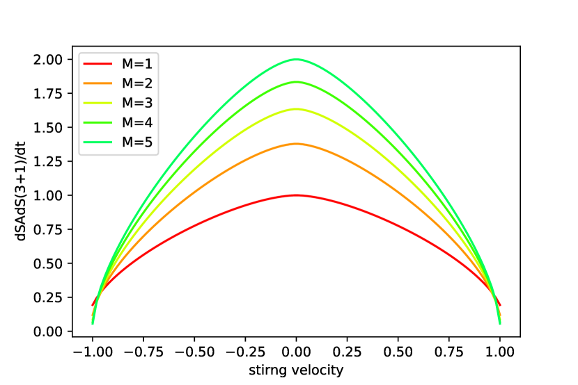
Figure 1: AdS₃₊₁: Action growth - string velocity

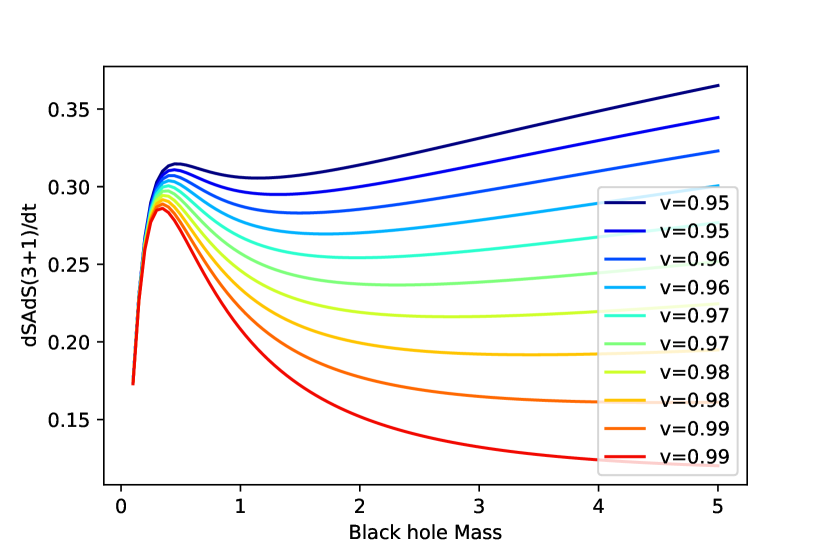
Figure 2: AdS₃₊₁: Action growth - Black hole mass

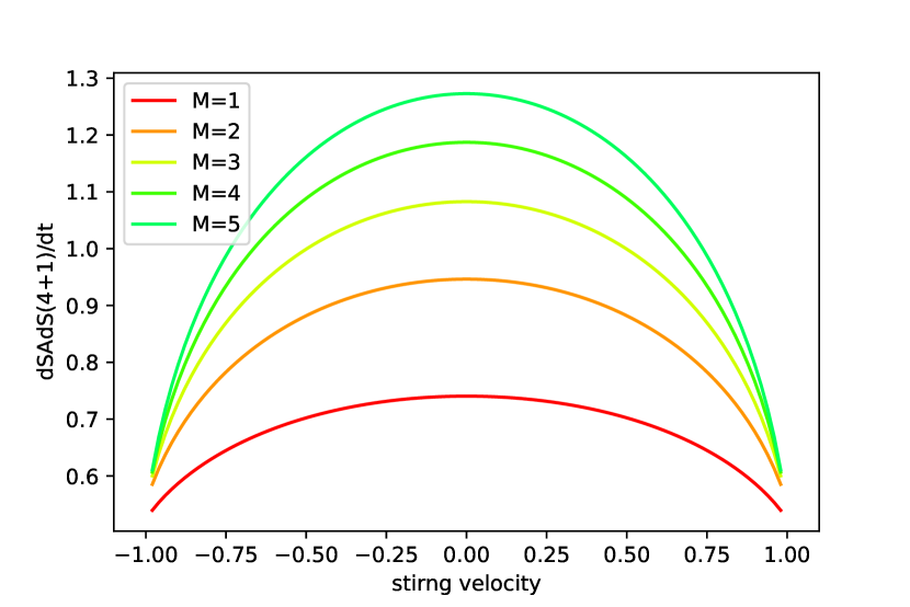
Figure 3: AdS₄₊₁: Action growth - string velocity

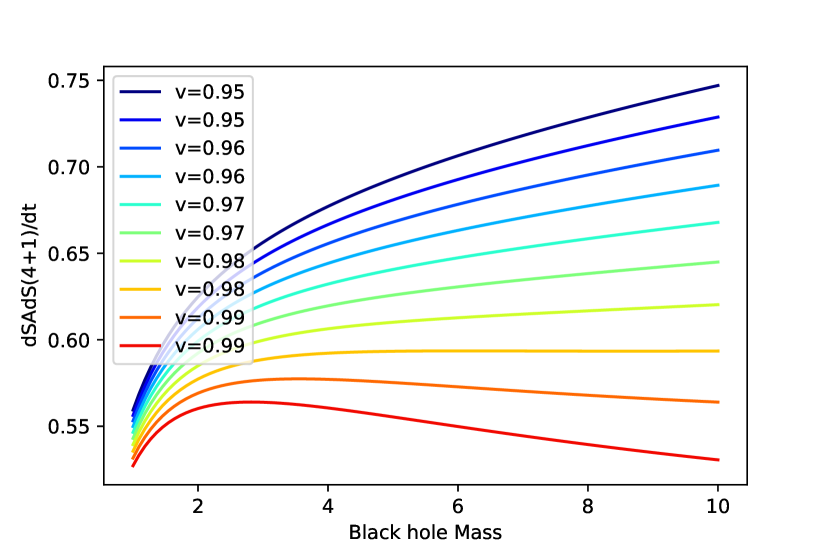
Figure 4: AdS₄₊₁: Action growth - Black hole mass

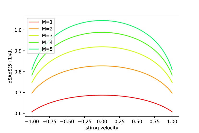
Figure 5: AdS₅₊₁: Action growth - string velocity

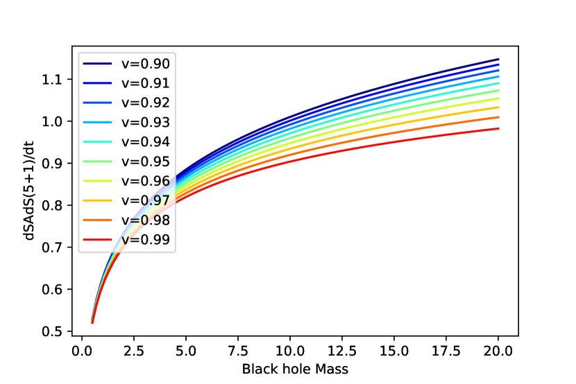
Figure 6: AdS₅₊₁: Action growth - Black hole mass

3 BTZ black holes

We consider the string moving in the BTZ black hole spacetime. The butterfly effects caused by a small perturbation on an asymptotic region in this black holes is studied in [130]. In this section we study the effect of the string moving on this spacetime geometry. The BTZ black hole is $(2+1)$-spacetime specified as

$$ds_{\text{BTZ}}^{2}=-f(r)dt^{2}+\frac{dr^{2}}{f(r)}+r^{2}\Big{(}d\phi-\frac{r_{+}r_{-}}{\ell_{\text{AdS}}r^{2}}dt\Big{)}^{2},\;f(r):=\frac{(r^{2}-r_{+}^{2})(r^{2}-r_{-}^{2})}{\ell_{\text{AdS}}^{2}r^{2}}.$$ (19)

The parameters $r_{\pm}$ are the inner and the outer horizon which is related to black hole mass $M$ and angular momentum $J$ by

$$M=(r_{+}^{2}+r_{-}^{2})/\ell_{\text{AdS}}^{2},\;J=2r_{+}r_{-}/\ell_{\text{AdS}}.$$ (20)

We rescale $r_{\text{(old)}}=r_{\text{(new)}}\ell_{\text{AdS}}$ and for $r_{\pm}$ and $t$ in the same way. This simplifies the expression and the metric becomes the original one times $\ell_{\text{AdS}}^{2}$. One edge of the string moves with velocity $v$. We parametrize the worldsheet as follows:

$$t=\tau,\;r=\sigma,\;\phi=v\tau+\xi(\sigma).$$ (21)

Since we here use the $\ell_{\text{AdS}}=1$ unit, the angular velocity of the string $\omega$ is $\omega=v/\ell_{AdS}=v$. The induced metric is

$$ds_{\text{BTZind}}^{2} =-\Big{(}f(\sigma)-\Big{(}v\sigma-\frac{r_{+}r_{-}}{\sigma}\Big{)}^{2}\Big{)}d\tau^{2}+\Big{(}\frac{1}{f(\sigma)}+\sigma^{2}\xi^{\prime}(\sigma)^{2}\Big{)}d\sigma^{2}$$

$$\qquad+2\Big{(}v\sigma-\frac{r_{+}r_{-}}{\sigma}\Big{)}\sigma\xi^{\prime}(\sigma)d\tau d\sigma,$$ (22)

$$f(\sigma) =\frac{(\sigma^{2}-r_{+}^{2})(\sigma^{2}-r_{-}^{2})}{\sigma^{2}}.$$ (23)

The Nambu-Goto Lagrangian is given by the determinant of this metric.

$$\mathcal{L}_{\text{BTZ}}=T_{\text{s}}\sqrt{1+f(\sigma)\sigma^{2}\xi^{\prime}(\sigma)^{2}-\frac{1}{f(\sigma)}\Big{(}v\sigma-\frac{J}{2\sigma}\Big{)}^{2}},$$ (24)

where angular momentum is rescaled as $J_{\text{(old)}}/\ell_{\text{AdS}}=:J$.

EOM and its solution

By the equation of motion,

$$\frac{d}{d\sigma}\Big{(}\frac{f(\sigma)\sigma^{2}\xi^{\prime}(\sigma)}{\mathcal{L}_{\text{BTZ}}/T_{\text{s}}}\Big{)}=0,\;c_{\xi}:=\frac{f(\sigma)\sigma^{2}\xi^{\prime}(\sigma)}{\mathcal{L}_{\text{BTZ}}/T_{\text{s}}},$$ (25)

$$\xi^{\prime}(\sigma)=\frac{c_{\xi}}{\sigma^{2}f(\sigma)}\sqrt{\frac{\sigma^{2}f(\sigma)-(v\sigma^{2}-J/2)^{2}}{\sigma^{2}f(\sigma)-c_{\xi}^{2}}}.$$ (26)

For this function to give the real values, the numerator and the denominator in the square root must have the same zero point. This condition leads that the denominator is zero when

$$\sigma=\sigma_{\text{H}}^{2}:=\frac{M-vJ}{1-V^{2}}.$$ (27)

This determines the integration constant as

$$c_{\xi}=|v\sigma_{\text{H}}^{2}-J/2|.$$ (28)

Then the square root of (26) is factorized by $(\sigma-\sigma_{\text{H}})$.

$$\xi^{\prime}(\sigma)=\frac{c_{\xi}}{\sigma^{2}f(\sigma)}\sqrt{\frac{(1-v^{2})(\sigma^{2}+\sigma_{\text{H}}^{2})-(M-vJ)}{\sigma^{2}+\sigma_{\text{H}}^{2}-M}}.$$ (29)

From the relation (25), the Lagrangian is

$$\frac{\mathcal{L}_{\text{BTZ}}}{T_{\text{s}}}=\sqrt{\frac{(1-v^{2})\sigma^{2}}{\sigma^{2}+\sigma_{\text{H}}^{2}-M}}.$$ (30)

Action

The development of the Nambu-Goto action is obtained by integrating this Lagrangian over the WDW patch,

$$\frac{1}{T_{\text{s}}}\frac{dS_{\text{NG}}}{dt}=\sqrt{1-v^{2}}\int_{r_{-}}^{r_{+}}d\sigma\frac{\sigma}{\sqrt{\sigma^{2}+\sigma_{\text{H}}^{2}-M}}=|r_{+}-vr_{-}|-|r_{-}-vr_{+}|.$$ (31)

In our scaling, $M=r_{+}^{2}+r_{-}^{2},\;J=2r_{+}r_{-}$, $r_{\pm}=\frac{1}{2}(\sqrt{M+J}\pm\sqrt{M-J})$. We express the above action by the parameter $M$ and $J$.

$$\frac{1}{T_{\text{s}}}\frac{dS_{\text{NG}}}{dt}=\frac{1}{2}\big{(}(1-v)\sqrt{M+J}+(1+v)\sqrt{M-J}\big{)}-\frac{1}{2}\big{|}(1-v)\sqrt{M+J}-(1+v)\sqrt{M-J}\big{|}.$$ (32)

This plot is shown in figures 8, 8, 10 and 10.

According to the results in the previous work [127], complexity growth is expected to take the maximum when the string is stationary. So it seems to be meaningful to see the dependence of the relative velocity between the black hole and the string. That dependence of the relative velocity is shown in figures 12 and 12. As expected, this tendency is seen in these plots. That is, the effect to complexity takes maximum when the relative velocity is zero for rotating black holes. The effect is larger for larger black holes as AdS₄ case [127].

Figure 8 and figure 8 show the velocity dependence for different angular momentums $J/M$. In the left figure 8 the peak position is shifted because of the black hole rotation. In the right figure 8, since the black hole rotates in the opposite direction to the string, the peak is shifted in the opposite side. Not only the peak position is shifted, we can also see that the peak value becomes smaller for a large shift. Note that in this case the effect of the probe string is exactly zero when the string motion reaches to the light speed.

Figure 10 also shows that the effect of the string is smaller for fast moving strings. And this is a monotonically increasing function of the black hole mass. This can be thought that this is because complexity defines how complex of the physical system. Then a larger system may have larger information.

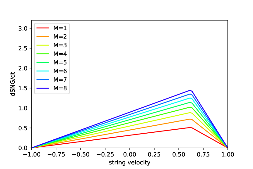
Figure 7: BTZ: Action growth - string velocity $J/M=0.9$ fixed

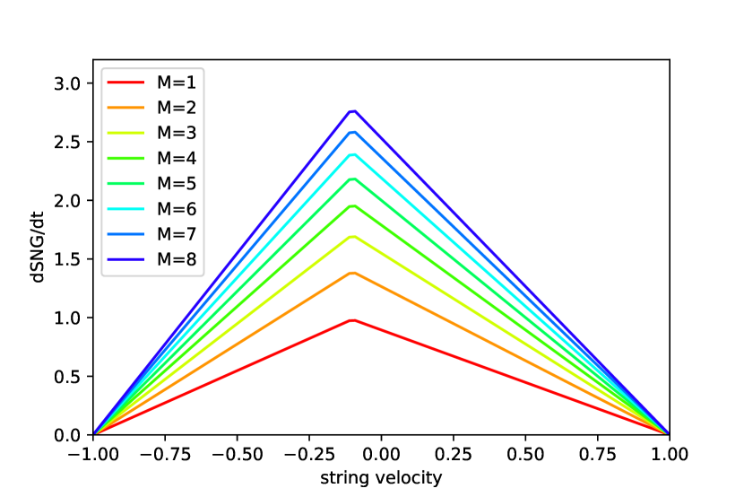
Figure 8: BTZ: Action growth - string velocity $J/M=-0.2$ fixed

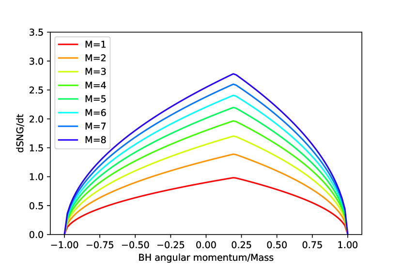
Figure 9: BTZ: Action growth - Black hole angular momentum/Mass

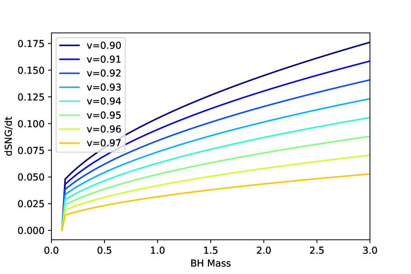
Figure 10: BTZ: Action growth - Black hole mass (small mass region)

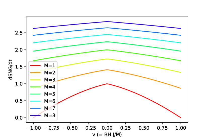
Figure 11: BTZ: Action growth - string velocity (relative velocity$=0$)

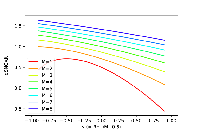
Figure 12: BTZ: Action growth - string velocity (relative velocity$=0.5$)

4 Kerr-AdS black holes

In this section we consider the Kerr-AdS black holes which are black hole solutions with angular momentum. General higher dimensional solution is known and that holographic correspondence is studied in [131, 132].

4.1 Four dimensional Kerr-AdS black holes

We consider here AdS black holes with angular momentum. The Einstein-Hilbert action of this black holes is studied in [97]. We study an effect of the probe string here. In the Boyer-Lindquist coordinates the four-dimensional Kerr-AdS black hole is given by

$$ds_{\text{KA4}}^{2} =-\frac{\Delta_{r}}{\rho^{2}}\Big{(}dt-\frac{a\sin^{2}\theta}{\Xi}d\phi\Big{)}^{2}+\frac{\rho^{2}}{\Delta_{r}}dr^{2}+\frac{\rho^{2}}{\Delta_{\theta}}d\theta^{2}+\frac{\Delta_{\theta}\sin^{2}\theta}{\rho^{2}}\Big{(}adt-\frac{r^{2}+a^{2}}{\Xi}d\phi\Big{)}^{2}$$ (33)

$$=-\Big{(}\frac{\Delta_{r}}{\rho^{2}}-\frac{\Delta_{\theta}\sin^{2}\theta}{\rho^{2}}a^{2}\Big{)}dt^{2}+\frac{\rho^{2}}{\Delta_{r}}dr^{2}+\frac{\rho^{2}}{\Delta_{\theta}}d\theta^{2}$$

$$\qquad+2\frac{a\Delta_{r}\sin^{2}\theta-a(r^{2}+a^{2})\Delta_{\theta}\sin^{2}\theta}{\rho^{2}\Xi}dtd\phi+\frac{(r^{2}+a^{2})^{2}\Delta_{\theta}\sin^{2}\theta-a^{2}\Delta_{r}\sin^{4}\theta}{\rho^{2}\Xi^{2}}d\phi^{2},\;$$ (34)

where

$$\Delta_{r} =(r^{2}+a^{2})(1+r^{2}/\ell_{\text{AdS}}^{2})-2mr,\;\Xi=1-a^{2}/\ell_{\text{AdS}}^{2},$$

$$\Delta_{\theta} =1-a^{2}\cos^{2}\theta/\ell_{\text{AdS}}^{2},\;\rho^{2}=r^{2}+a^{2}\cos^{2}\theta.$$

The physical mass and the angular momentum are $M=m/(G_{\text{N}}\Xi)$ and $J=ma/(G_{\text{N}}\Xi)$. The above metric is related with the AdS coordinates $\Phi$ (see also (4.11) of [133]) as follows. Put the AdS boundary coordinates as $t$ and $\Omega$ and they are related by $\Phi=\phi+\Omega t$. In this coordinate, the first and the last terms of eq.(33) are, at $\theta=\pi/2$,

$$-r^{2}\ell_{\text{AdS}}^{-2}\Big{[}dt-\frac{a}{\Xi}d\phi\Big{]}^{2} =-r^{2}\ell_{\text{AdS}}^{-2}\Big{[}\Big{(}1-\frac{a\Omega}{\Xi}\Big{)}dt-\frac{a}{\Xi}d\Phi\Big{]}^{2},$$

$$\frac{1}{r^{2}}\Big{[}adt-\frac{r^{2}}{\Xi}d\phi\Big{]}^{2} =\frac{1}{r^{2}}\Big{[}\Big{(}a-\frac{r^{2}\Omega}{\Xi}\Big{)}dt-\frac{r^{2}}{\Xi}d\Phi\Big{]}^{2}.$$

In order for these terms to give the form of AdS metric at $r\rightarrow\infty$, the cross terms from these terms should cancel. Then, the parameter $\Omega$ is determined

$$\phi=\Phi-a\ell_{\text{AdS}}^{-2}t.$$ (35)

We consider a string moving in this spacetime. In the following we use the rescaled coordinates so that $\ell_{\text{AdS}}=1$. We assume that the string moves on the great circle of the subspace $S^{2}$: $\theta=\pi/2$. We parametrize the string worldsheet as

$$t=\tau,\;r=\sigma,\;\Phi=V\tau+\xi(\sigma).$$ (36)

Taking into account the relation (35), the above is

$$t=\tau,\;r=\sigma,\;\phi=(V-a)\tau+\xi(\sigma):=v\tau+\xi(\sigma).$$ (37)

We defined the shifted velocity as $v:=V-a$ which is used in the following calculation while the original $V$ is the string velocity. Let us define a function

$$\Delta(\sigma):=\Delta_{r}(r=\sigma)=(\sigma^{2}+a^{2})(1+\sigma^{2})-2m\sigma.$$ (38)

The induced metric is

$$ds_{\text{KA4ind}}^{2} =-\Big{(}\frac{\Delta}{\sigma^{2}}-\frac{a^{2}}{\sigma^{2}}-2\frac{av}{\sigma^{2}}\frac{\Delta-(\sigma^{2}+a^{2})}{\Xi}-v^{2}\frac{(\sigma^{2}+a^{2})^{2}-a^{2}\Delta}{\sigma^{2}\Xi^{2}}\Big{)}d\tau^{2}$$

$$\qquad+\Big{(}\frac{\sigma^{2}}{\Delta}+\frac{(\sigma^{2}+a^{2})^{2}-a^{2}\Delta}{\sigma^{2}\Xi^{2}}\xi^{\prime 2}\Big{)}d\sigma^{2}$$

$$\qquad+\frac{2\xi^{\prime}}{\sigma^{2}\Xi}\Big{(}a(\Delta-(\sigma^{2}+a^{2}))+v\frac{(\sigma^{2}+a^{2})^{2}-a^{2}\Delta}{\Xi}\Big{)}d\tau d\sigma.$$ (39)

We define functions for simplicity:

$$F:=\Delta-(\sigma^{2}+a^{2}),\;G:=(\sigma^{2}+a^{2})^{2}-a^{2}\Delta.$$ (40)

Its determinant is

$$-\det[g_{\text{KA4ind}}] =\Big{(}\frac{\Delta}{\sigma^{2}}-\frac{a^{2}}{\sigma^{2}}-2\frac{av}{\sigma^{2}}\frac{F}{\Xi}-v^{2}\frac{G}{\sigma^{2}\Xi^{2}}\Big{)}\Big{(}\frac{\sigma^{2}}{\Delta}+\frac{G}{\sigma^{2}\Xi^{2}}\xi^{\prime 2}\Big{)}+\frac{\xi^{\prime 2}}{\sigma^{4}\Xi^{2}}\Big{(}aF+v\frac{G}{\Xi}\Big{)}^{2}.$$ (41)

Further we define

$$H(\sigma):=\frac{\Delta}{\sigma^{2}}-\frac{a^{2}}{\sigma^{2}}-2\frac{av}{\sigma^{2}}\frac{F}{\Xi}-v^{2}\frac{G}{\sigma^{2}\Xi^{2}},\;I(\sigma):=\Big{(}aF+v\frac{G}{\Xi}\Big{)}^{2}.$$ (42)

EOM and Lagrangian

The Lagrangian and the equation of motion is

$$\frac{\mathcal{L}_{\text{KA4}}}{T_{\text{s}}}=\Big{[}H\Big{(}\frac{\sigma^{2}}{\Delta}+\frac{G}{\sigma^{2}\Xi^{2}}\xi^{\prime 2}\Big{)}+\frac{\xi^{\prime 2}}{\sigma^{4}\Xi^{2}}I\Big{]}^{1/2},\;\;\frac{1}{T_{\text{s}}}\frac{\partial\mathcal{L}_{\text{KA4}}}{\partial\xi^{\prime}(\sigma)}=\frac{\xi^{\prime}/(\sigma^{4}\Xi^{2})}{\mathcal{L}_{\text{KA4}}/T_{\text{s}}}[\sigma^{2}HG+I]=:c_{\xi}.$$ (43)

Solving it for $\xi^{\prime}(\sigma)$, we obtain

$$\xi^{\prime}=c_{\xi}\sigma^{4}\Xi^{2}\sqrt{\frac{\sigma^{2}H/\Delta}{(\sigma^{2}HG+I)(\sigma^{2}HG+I-c_{\xi}^{2}\sigma^{4}\Xi^{2})}}.$$ (44)

We impose the reality condition as before. We need to find the zero of

$$\sigma^{2}H =\Delta-a^{2}-2av\frac{\Delta-(\sigma^{2}+a^{2})}{\Xi}-v^{2}\frac{(\sigma^{2}+a^{2})^{2}-a^{2}\Delta}{\Xi^{2}}$$

$$=\Delta(\sigma)\Big{(}1-\frac{av}{\Xi}\Big{)}^{2}-\Big{(}a-\frac{v(\sigma^{2}+a^{2})}{\Xi}\Big{)}^{2}.$$ (45)

We denote this solution as $\sigma=\sigma_{\text{H}}$. Actually $\sigma^{2}H(\sigma)=0$ has a unique solution at positive region. The denominator must be zero coincidentally. This condition determines the integration constant $c_{\xi}$:

$$0=I(\sigma_{\text{H}})^{2}-c_{\xi}^{2}\Xi^{2}\sigma_{\text{H}}^{4}I(\sigma_{\text{H}}),\;\;\qquad\therefore c_{\xi}^{2}\Xi^{2}=I(\sigma_{\text{H}})/\sigma_{\text{H}}^{4}.$$ (46)

Substituting this constant into the above, we obtain

$$\xi^{\prime}(\sigma)=c_{\xi}\sigma^{4}\Xi^{2}\sqrt{\frac{\sigma^{2}H(\sigma)/\Delta(\sigma)}{(\sigma^{2}H(\sigma)G(\sigma)+I(\sigma))(\sigma^{2}H(\sigma)G(\sigma)+I(\sigma)-I(\sigma_{\text{H}})\sigma^{4}/\sigma_{\text{H}}^{4})}},$$ (47)

and the Lagrangian

$$\frac{\mathcal{L}_{\text{KA4}}}{T_{\text{s}}}=\frac{[\sigma^{2}HG+I]}{c_{\xi}\sigma^{4}\Xi^{2}}\xi^{\prime}(\sigma)=\sqrt{\frac{(\sigma^{2}H(\sigma)G(\sigma)+I(\sigma))\sigma^{2}H(\sigma)/\Delta(\sigma)}{\sigma^{2}H(\sigma)G(\sigma)+I(\sigma)-I(\sigma_{\text{H}})\sigma^{4}/\sigma_{\text{H}}^{4}}}.$$ (48)

Action

The outer and the inner horizon are the smaller and the larger solutions of $\Delta_{r}(r)=0$, respectively. The integral in the WDW patch is

$$\frac{1}{T_{\text{s}}}\int_{r_{-}}^{r_{+}}d\sigma\mathcal{L}_{\text{KA4}}=\int_{r_{-}}^{r_{+}}d\sigma\sqrt{\frac{\sigma^{2}H(\sigma)(\sigma^{2}H(\sigma)G(\sigma)+I(\sigma))}{\Delta(\sigma)(\sigma^{2}H(\sigma)G(\sigma)+I(\sigma)-I(\sigma_{\text{H}})\sigma^{4}/\sigma_{\text{H}}^{4})}}.$$ (49)

The numerical calculation gives the results shown in figures 14, 14, 16 and 16.

The first two figures, figure 14 and figure 14, show the string velocity dependence in different masses. The left one is the result for $a=0.1$. The peak position is shifted to the right side. The right figure is, on the other hand, the result for a black hole with angular momentum of the opposite direction $a=-0.2$. The peak position is shifted to the other side. This behavior is consistent with the property that complexity is larger as the probe string motion is slower. That is, the effect takes the peak value when the relative velocity between the string and the black hole is zero. Not only that we can also the peak value decreases as the shift becomes larger similar to the BTZ black hole case.

Figure 16 is the dependence of the angular momentum per black hole mass. This figure also shows that the effect to complexity is smaller as the string moves faster. And It also shows the tendency that complexity is larger when the relative velocity is smaller because in this plot the string velocity is positive and the effect of complexity is larger in the positive region of the graph.

Figure 16 shows the mass dependence. As usual this is a increasing function of black hole mass. The faster string gives the small effect to complexity. But there is an unusual behavior in the small mass region where the extremum value appears.

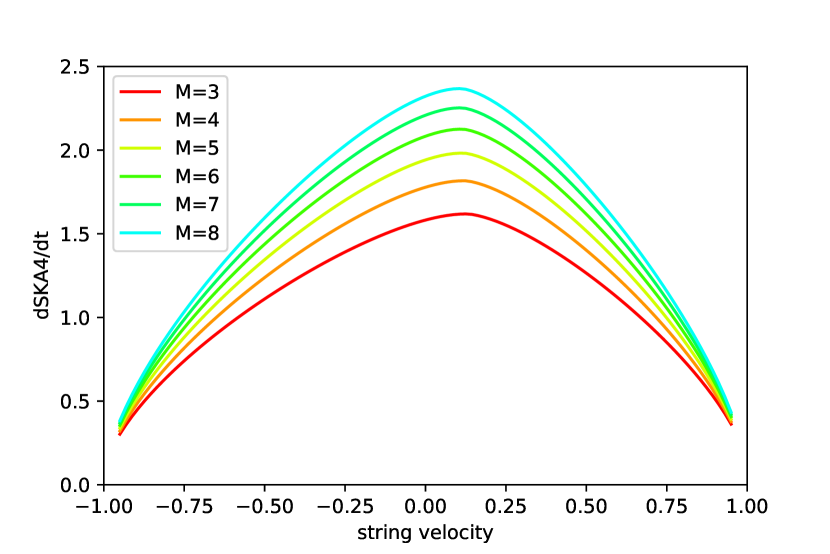
Figure 13: Kerr-AdS₃₊₁: Action growth - string velocity ($a=0.1$)

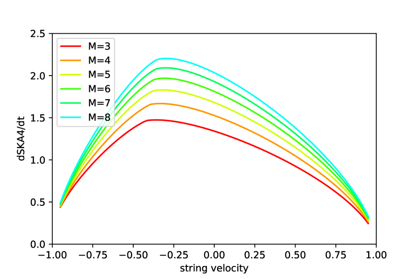
Figure 14: Kerr-AdS₃₊₁: Action growth - string velocity ($a=-0.2$)

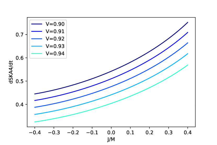
Figure 15: Kerr-AdS₃₊₁: Action growth - Black hole $J/M$ ($m=5$)

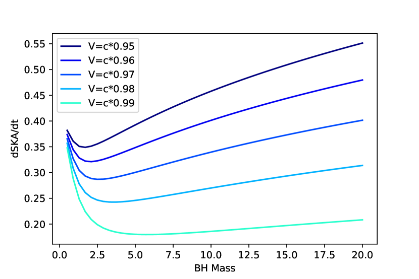
Figure 16: Kerr-AdS₃₊₁: Action growth - Black hole mass ($a=0.1$)

4.2 Five dimensional Kerr-AdS black holes

The (4+1)-dimensional Kerr-AdS black hole is described by (see references [133, 134, 132, 135])

$$ds_{\text{KA5}}^{2} =-\frac{\Delta_{r}}{\rho^{2}}\Big{(}dt-\frac{a\sin^{2}\theta}{\Xi_{a}}d\phi_{1}-\frac{b\cos^{2}\theta}{\Xi_{b}}d\phi_{2}\Big{)}^{2}$$

$$+\frac{\Delta_{\theta}\sin^{2}\theta}{\rho^{2}}\Big{(}adt-\frac{r^{2}+a^{2}}{\Xi_{a}}d\phi_{1}\Big{)}^{2}+\frac{\Delta_{\theta}\cos^{2}\theta}{\rho^{2}}\Big{(}bdt-\frac{r^{2}+b^{2}}{\Xi_{b}}d\phi_{2}\Big{)}^{2}$$

$$+\frac{\rho^{2}}{\Delta_{r}}dr^{2}+\frac{\rho^{2}}{\Delta_{\theta}}d\theta^{2}+\frac{1+r^{2}}{r^{2}\rho^{2}}\Big{(}abdt-\frac{b(r^{2}+a^{2})\sin^{2}\theta}{\Xi_{a}}d\phi_{1}-\frac{a(r^{2}+b^{2})\cos^{2}\theta}{\Xi_{b}}d\phi_{2}\Big{)}^{2},$$ (50)

where

$$\rho^{2}(r)=r^{2}+a^{2}\cos^{2}\theta+b^{2}\sin^{2}\theta,$$

$$\Delta_{r}(r)=\frac{1}{r^{2}}(r^{2}+a^{2})(r^{2}+b^{2})(r^{2}+1)-2m,\qquad\Delta_{\theta}(\theta)=1-a^{2}\cos^{2}\theta-b^{2}\sin^{2}\theta,$$

$$\Xi_{a}=1-a^{2},\qquad\Xi_{b}=1-b^{2}.$$

The parameters here is related to the physical mass and the angular momentum as ([134])

$$M=\frac{3\pi m}{4\Xi_{1}\Xi_{2}},\;J_{i}=\frac{\pi a_{i}m}{2\Xi_{i}(1+r_{+}^{2})}.$$ (51)

We study the $a\neq 0$ case and the $b\neq 0$ case separately. These correspond to black holes rotating around different axises with coordinates $\phi_{1}$ and $\phi_{2}$. As before we assume that the string moves in the great circle: $\theta=\pi/2$.

4.2.1 $a\neq 0$ case

First we consider the case where only $a$ is nonzero. In this case the string rotates around the same axis to the black hole.

$$ds_{\text{KA5a}}^{2} =-\frac{\Delta_{ra}}{r^{2}}\Big{(}dt-\frac{a}{\Xi_{a}}d\phi_{1}\Big{)}^{2}+\frac{r^{2}}{\Delta_{ra}}dr^{2}+\frac{1}{r^{2}}\Big{(}adt-\frac{r^{2}+a^{2}}{\Xi_{a}}d\phi_{1}\Big{)}^{2},$$ (52a)

$$\Delta_{ra} =(r^{2}+a^{2})(r^{2}+1)-2m.$$ (52b)

This looks the same form to the four-dimensional Kerr-AdS case except that the function $\Delta_{r}(r)$ is replaced with $\Delta_{ra}(r)$ (the second term does not depend on $r$). We needs the same shift (35) to relate the velocity parameter $v$ to the string velocity $V$: $v=V-a$ The parametrization of the string worldsheet is

$$t=\tau,\;r=\sigma,\;\Phi=V\tau+\xi(\sigma).$$ (53)

EOM and its solution

The calculation of the induced metric and the NG action are performed in the same way as the Kerr-AdS₃₊₁ case. So the Lagrangian is the same form to (48) except that $\Delta(r)$ is replaced with $\Delta_{a}$:

$$\frac{\mathcal{L}_{\text{KA5a}}}{T_{\text{s}}}=\sqrt{\frac{(\sigma^{2}H(\sigma)G(\sigma)+I(\sigma))\sigma^{2}H(\sigma)/\Delta_{a}(\sigma)}{\sigma^{2}H(\sigma)G(\sigma)+I(\sigma)-I(\sigma_{\text{H}})\sigma^{4}/\sigma_{\text{H}}^{4}}},$$ (54)

where

$$\Delta_{a}(\sigma) :=(\sigma^{2}+a^{2})(\sigma^{2}+1)-2m,$$ (55a)

$$F(\sigma) :=\Delta_{a}(\sigma)-(\sigma^{2}+a^{2}),\qquad G(\sigma) :=(\sigma^{2}+a^{2})^{2}-a^{2}\Delta_{a}(\sigma),$$ (55b)

$$H(\sigma) :=\frac{\Delta_{a}(\sigma)}{\sigma}-\frac{a^{2}}{\sigma}-2\frac{av}{\Xi_{a}}-v^{2}\frac{G(\sigma)}{\sigma^{2}\Xi^{2}},\qquad I(\sigma) :=\Big{(}aF(\sigma)+v\frac{G}{\Xi}\Big{)}^{2}.$$ (55c)

The inner and the outer horizons are determined by

$$\Delta_{ra}(r_{\pm})=0.$$ (56)

Action

The action integrated over the WDW patch is

$$\frac{dS_{\text{NG}}}{dt}=\int_{r_{-}}^{r_{+}}d\sigma\sqrt{\frac{(\sigma^{2}H(\sigma)G(\sigma)+I(\sigma))\sigma^{2}H(\sigma)/\Delta_{a}(\sigma)}{\sigma^{2}H(\sigma)G(\sigma)+I(\sigma)-I(\sigma_{\text{H}})\sigma^{4}/\sigma_{\text{H}}^{4}}}.$$ (57)

This integration is performed by the numerical calculation. The result shows the string velocity dependence, the black hole angular momentum dependence and the mass dependence.

The velocity dependence is shown in figure 18 and figure 18. We can see as usual the effect to complexity is larger for larger mass and the effect is maximum when the string is stationary. But the difference for different values of parameter $a$ disappears.

The angular momentum per unit mass ($a=J/M$) dependence is shown in figure 20. Similar to the velocity dependence, a sharp slope tends to disappear. There is a universal behavior — the effect of the string is small when the relative velocity is large.

The mass dependence is shown in figure 20. Basically the effect increases according to the black hole mass but this changes to the decreasing function if once the string velocity exceeds the threshold (it is almost the light speed $\approx 0.98c$).

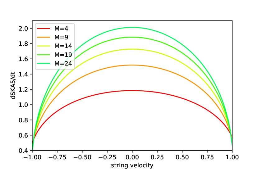
Figure 17: Kerr-AdS₄₊₁: Action growth - velocity ($a=0.1$)

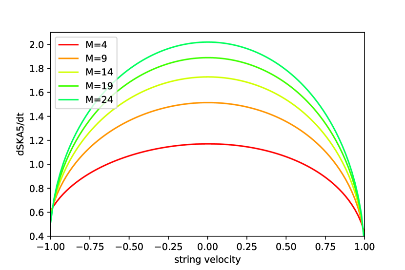
Figure 18: Kerr-AdS₄₊₁: Action growth - $m$ ($a=-0.2$)

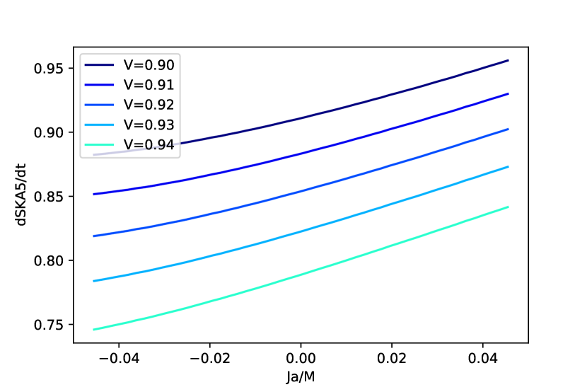
Figure 19: Kerr-AdS₄₊₁: Action growth - Black hole $J_{a}/M$ ($m=5$)

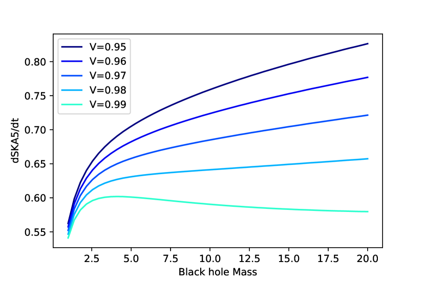
Figure 20: Kerr-AdS₄₊₁: Action growth - Black hole mass ($a=0.1$)

4.2.2 $b\neq 0$ case

Next let us consider the $b\neq 0$ case. In this case the string moves in the axis to the black hole. The metric becomes

$$ds_{\text{KA5b}}^{2} =-\frac{\Delta_{rb}}{r^{2}+b^{2}}dt^{2}+\frac{r^{2}+b^{2}}{\Delta_{rb}}dr^{2}+\frac{r^{4}(1-b^{2})+b^{2}r^{2}(1+r^{2})}{r^{2}+b^{2}}d\phi_{1}^{2},$$

$$\qquad\Delta_{rb}=(r^{2}+b^{2})(r^{2}+1)-2m,$$

$$=-\Big{(}r^{2}+1-\frac{2m}{r^{2}+b^{2}}\Big{)}dt^{2}+\Big{(}r^{2}+1-\frac{2m}{r^{2}+b^{2}}\Big{)}^{-1}dr^{2}+r^{2}d\phi_{1}^{2}.$$ (58)

Since $\Xi_{a}=1$, from eq.(51) the angular momentum per black hole mass is

$$\frac{J_{b}}{M}=\frac{2}{3}\frac{b}{1+r_{+}^{2}}.$$ (59)

We choose the same parametrization as before:

$$\tau=t,\;r=\sigma,\;\phi_{1}=v\tau+\xi(\sigma).$$ (60)

Note that the above metric is already the AdS form. Then one does not need to shift the velocity (35) to relate the string velocity to the parameter $v$ ($V=v$). The induced metric is

$$ds_{\text{KA5b:ind}}^{2} =-f(\sigma)d\tau^{2}+\frac{d\sigma^{2}}{f(\sigma)}+\sigma^{2}(vd\tau+\xi^{\prime}d\sigma)^{2};\;f(\sigma):=1+\sigma^{2}-\frac{2m}{\sigma^{2}+b^{2}},$$

$$=-(f(\sigma)-v^{2}\sigma^{2})d\tau^{2}+\Big{(}\frac{1}{f(\sigma)}+\sigma^{2}\xi^{\prime 2}\Big{)}d\sigma^{2}+2v\sigma^{2}\xi^{\prime}d\tau d\sigma.$$ (61)

EOM and its solution

This induced metric is the same form as AdS_n+1 (4) case except that the function $f(\sigma)$ is replaced. Then, the equation of motion is now obtained only by replacing with the old $f(\sigma)$ with the new one,

$$\xi^{\prime}(\sigma)=\frac{c_{\xi}}{\sigma^{2}f(\sigma)}\frac{\mathcal{L}_{\text{KA5b}}}{T_{\text{s}}}=\frac{c_{\xi}}{\sigma^{2}f(\sigma)}\sqrt{\frac{\sigma^{2}f(\sigma)-v^{2}\sigma^{4}}{\sigma^{2}f(\sigma)-c_{\xi}^{2}}},\;f(\sigma)=1+\sigma^{2}-\frac{2m}{\sigma^{2}+b^{2}}.$$ (62)

The reality condition in the square root should be imposed. The numerator is

$$0=1+(1-v^{2})\sigma^{2}-2m/(\sigma^{2}+b^{2})$$

$$\Rightarrow(1-v^{2})\sigma^{4}+(1+(1-v^{2})b^{2})\sigma^{2}+b^{2}-2m=0.$$ (63)

Since $D=(1+(1-v^{2})b^{2})^{2}+4(1-v^{2})(2m-b^{2})=(1-(1-v^{2})b^{2})^{2}+8m(1-v^{2})>0$, this equation certainly has real solutions. $\sigma_{\text{H}}$ denotes a positive one of them:

$$\sigma_{\text{H}}^{2}=-\frac{1+(1-v^{2})b^{2}}{2}+\frac{1}{2}\sqrt{(1-(1-v^{2})b^{2})^{2}+8m(1-v^{2})}.$$ (64)

From the condition for the denominator, the constant $c_{\xi}$ is determined as $c_{\xi}^{2}=\sigma_{\text{H}}^{2}f(\sigma_{\text{H}})$. The Lagrangian becomes

$$\frac{\mathcal{L}_{\text{KA5b}}}{T_{\text{s}}} =\sqrt{\frac{\sigma^{2}f(\sigma)-v^{2}\sigma^{4}}{\sigma^{2}f(\sigma)-\sigma_{\text{H}}^{2}f(\sigma_{\text{H}})}}$$

$$=\sigma\sqrt{\frac{(1-v^{2})(\sigma^{2}+\sigma_{\text{H}}^{2}+b^{2})+1}{(\sigma^{2}+b^{2})(\sigma^{2}+\sigma_{\text{H}}^{2}+1)-2mb^{2}/(\sigma_{\text{H}}^{2}+b^{2})}}.$$ (65)

The horizon is determined by

$$\Delta_{rb}(r)=0\qquad\therefore r_{\text{h}}=\Big{(}-\frac{1+b^{2}}{2}+\frac{1}{2}\sqrt{(1-b^{2})^{2}+8m}\Big{)}^{1/2}.$$ (66)

Action

Then the development of the NG action obtained by integrating over the WDW patch is

$$\frac{dS_{\text{NG}}}{dt} =\int_{0}^{r_{\text{h}}}d\sigma\sigma\sqrt{\frac{(1-v^{2})(\sigma^{2}+\sigma_{\text{H}}^{2}+b^{2})+1}{(\sigma^{2}+b^{2})(\sigma^{2}+\sigma_{\text{H}}^{2}+1)-2mb^{2}/(\sigma_{\text{H}}^{2}+b^{2})}}$$

$$=\frac{1}{2}\int_{0}^{r_{\text{h}}^{2}}d\sigma^{2}\sqrt{\frac{(1-v^{2})(\sigma^{2}+\sigma_{\text{H}}^{2}+b^{2})+1}{(\sigma^{2}+b^{2})(\sigma^{2}+\sigma_{\text{H}}^{2}+1)-2mb^{2}/(\sigma_{\text{H}}^{2}+b^{2})}}.$$ (67)

The figures 22, 22, 24 and 24 show the result of the numerical calculation.

The velocity dependence is shown in figure 22 and figure 22. As usual the effect to complexity takes extremum when string is stationary. There is an abnormal behavior in the vicinity of the light speed. It tends to increase a bit in the maximum of the velocity. Because of the reality condition the velocity can not reach to the light speed. This restricted region becomes narrow according to in creasing the absolute value of $b$. This is a new phenomena we found.

The dependence on the angular momentum is shown in figure 24. Since the string rotates in a different axis, the relative velocity never becomes zero. Then this behaves very differently from the previous ones.

Figure 24 shows the mass dependence. The difference between different velocities ceases and there is no extremum point in this case. While in the small mass region fast strings gives the large effect, in the large mass region the slower strings the larger effect as usual.

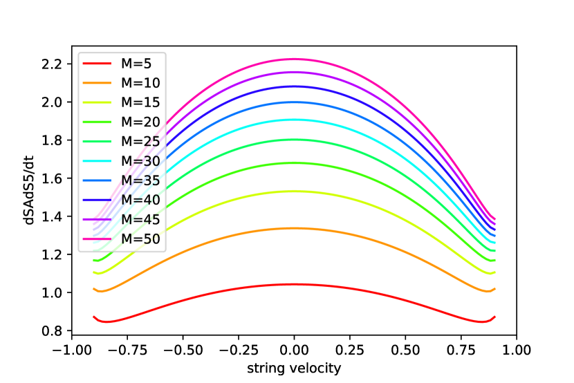
Figure 21: Kerr-AdS₄₊₁: Action growth - velocity ($b=0.1$)

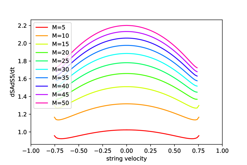
Figure 22: Kerr-AdS₄₊₁: Action growth - velocity ($b=-0.2$)

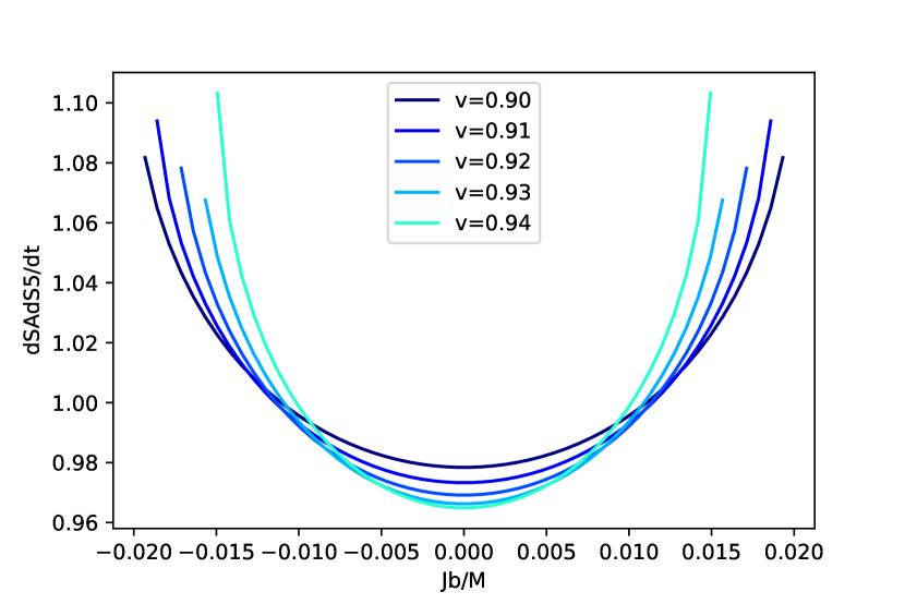
Figure 23: Kerr-AdS₄₊₁: Action growth - velocity ($b=0.1$)

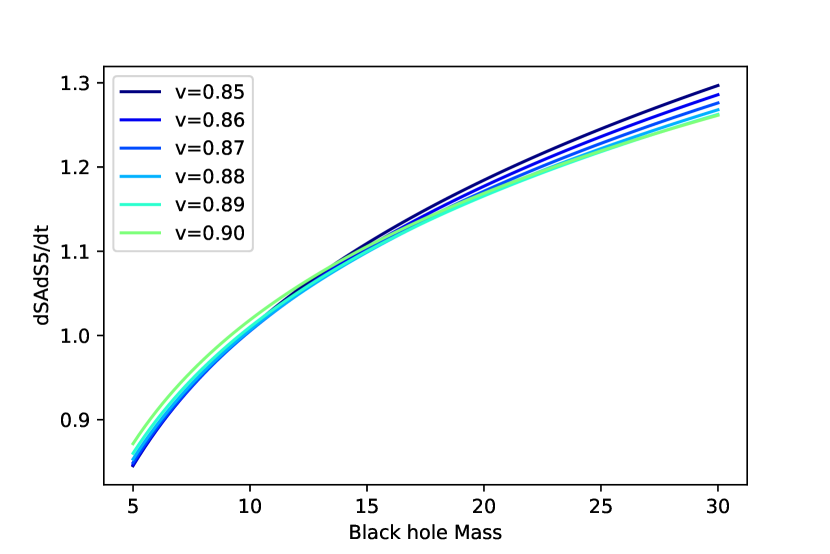
Figure 24: Kerr-AdS₄₊₁: Action growth - Black hole mass ($b=0.1$)

5 Discussion

5.1 Summary

We have seen the effect of the probe string in BTZ, AdS₃₊₁, AdS₄₊₁, AdS₅₊₁ and Kerr-AdS black hole spacetime. The previous work [127] revealed the effect of the probe string in different masses and string velocities. We could confirm this result and that is a universal behavior in more broad type of black holes. More specifically, complexity shows different behavior according to the string velocity, black hole mass and the spacetime dimension. Let us summarize these dependence and its physical interpretation here.

Velocity dependence

A stationary string gives the maximal complexity growth. Complexity decreases as the probe string moves faster. It seems to contradict the physical intuition because complexity measures how difficult to create the target state from the initial state which is usually stationary. The same phenomenon was found also in the previous work [127]. Then we can conclude that this is a universal property of complexity.

The position of the maximum is shifted in the rotating black hole. This is thought to be derived from the relative velocity between the string velocity and the black hole angular momentum. That is, the effect to complexity is larger when the relative velocity is smaller. The maximum value also decreases as the maximum point moves from the center by this shift. Near the light speed there is also an interesting phenomena in the mass dependence as stated below.

Let us note that the universal property of complexity stated above does not stem from the time delation of relativistic phenomena. Figures 8, 8, 14 and 14 show the peak position shifts according the relative velocity between the black hole and the probe string. Since we calculated the NG action on the rest flame, the peak locates at $v=0$ if this behavior stems from the time dilation. We can also see that if this behavior derives from the Lorentz factor $\sqrt{1-v^{2}}$, it does not behave linearly as BTZ cases (figure 8 and figure 8).

Mass dependence

Complexity basically tends to increase according the mass. This can be thought that this is because complexity defines how complex of the physical system.

A remarkable phenomenon occurs in the vicinity of the light speed. In the lower dimension, AdS₃₊₁ and the AdS₄₊₁, the dependence on black hole mass has the maximum point for near light speed strings. That maximum disappears for higher dimension as shown in the AdS₅₊₁ dimensional case 6.

In lower dimension, AdS_n+1≤5 the mass dependence can be a decreasing function of mass for a near light speed string.

Dimensionality dependence

As the spacetime dimension becomes higher, the peak of the dependence on the string velocity becomes smooth. Especially, in three dimensional case, the velocity dependence in BTZ black holes forms a broken line. As the dimensionality becomes higher this slope tend to become gentle.

We can conclude that the effect of the probe string becomes insensitive in higher dimensions. It can be intuitively explained as follows. Although the Nambu-Goto action is proportional to the two dimensional world volume in whole spacetime, we restrict the motion of the string in $S^{1}$ subspace of a specific plane. In order to remove this restriction, we investigate in section 4.2.2 the case where string moves around a different axis to the black hole angular momentum. As expected a new phenomena was found. That is, the dependence on the string velocity does not decrease near the light speed (see figs 22 and 22). Furthermore, the difference of the dependence on mass in various string velocities disappears in this case (see fig 24).

Maximum value

According to the results in sec.2 (figures 2, 4 and 6), the plots of the velocity dependence not only becomes smoother, but its maximum value also looks to decrease. Let us confirm whether this behavior is universal. We focus on AdS_n+1 black holes. We know already that the effect of the string is maximum when the string velocity is zero. For $v=0$, the Lagrangian (13) is unity. The integral depends only on the horizon:

$$\frac{\mathcal{L}_{\text{AdS(n+1)}}}{T_{\text{s}}}=r_{\text{h}}.$$ (68)

The horizon $r_{\text{h}}$ is determined by (see the metric function (2))

$$0=f(r)=1-\frac{16\pi}{(n-1)\Omega_{n-1}}\frac{M}{r^{n-2}}+r^{2}\Rightarrow r^{n}+r^{n-2}-\frac{8\pi^{-n/2+1}\Gamma(n/2)}{n-1}M=0.$$ (69)

The maximum value of the NG action in diverse dimensions is plotted in figure 26.

There is a difficulty for the charged case, as I explain later below of eq.(72). But only the maximum value can be obtained in the same way as the uncharged case. We focus on the extremal black holes. The Lagrangian is again unity and the action is equal to the horizon. This horizon is determined in the same way by

$$r^{n}+r^{n-2}-\frac{4\pi^{-n/2+1}\Gamma(n/2)}{n-1}\Big{(}2M-\frac{Q^{2}}{r}\Big{)}=0.$$ (70)

Given a charge, the extremal mass is determined by setting the minimum value of the left hand side (70) is zero. The dimensionality dependence of the maximum value of the NG action for extremal black holes is plotted in figure 26. By this plots we see that the maximum value decreases at lower dimensions. Furthermore, the minimum point approaches ten-dimension for sufficiently large charges.

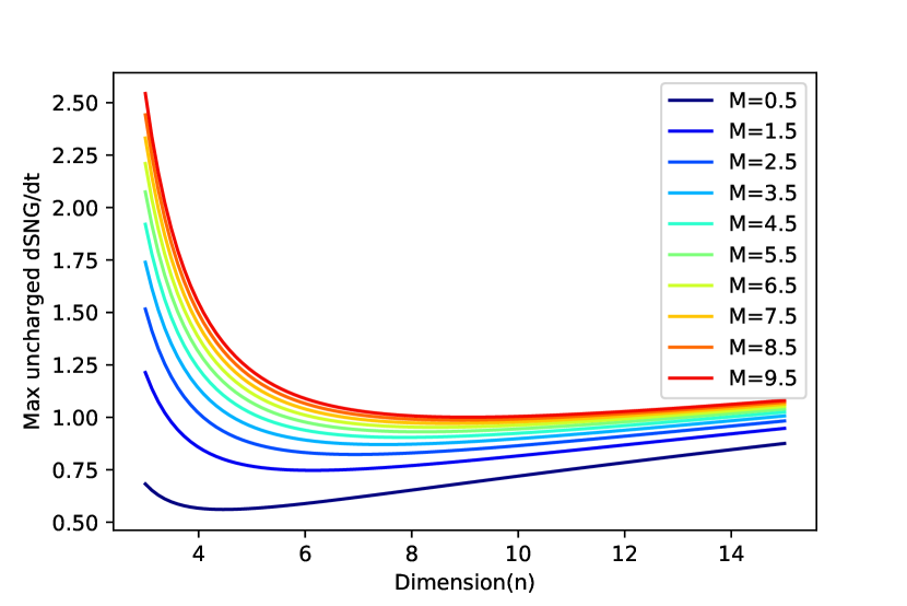
Figure 25: Maximum of the action growth in diverse dimensions (uncharged case)

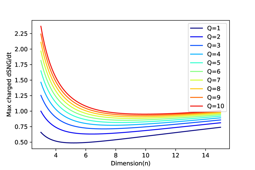
Figure 26: Maximum of the action growth in diverse dimensions (charged case)

5.2 Future direction

In this work we considered the effect of the probe string. That corresponds to the introduction of a kind of nonlocal operator — a Wilson loop. We first expect the generalization of the dimension. Several higher dimensional local operators can be added. Especially, the co-dimension local operator, interface, is an interesting object. This local operators realized in a system consisting of two kind branes — D3/D5. Since complexity is known to have a nonlocal property, it must be useful to use such kind of operators to study the property of complexity. Some interesting properties of the nonlocal operators in BTZ black holes are already found in [118] and complexity growth of defect theory is studied in [136]. One suggest is to study the effect of these nonlocal operators in the diverse kinds of black holes.

In (1) we restrict the case for uncharged AdS black holes. The growth of the Einstein-Hilbert action for charged case is studied in [137]. I would like to study the nonlocal operators in these kinds of black holes. The adding of the charge is an important future work since it is related to check whether the complexity growth satisfies the Lloyd bound [73, 114]. But in this case a difficulty occurs. The metric function in this case is

$$ds_{\text{AdS${}_{n+1}$}}^{2} =-f(r)dt^{2}+\frac{dr^{2}}{f(r)}+r^{2}d\Omega_{n-1},$$ (71a)

$$f(r) =1-\frac{8\pi}{(n-1)\Omega_{n-1}}\Big{(}\frac{2GM}{r^{n-2}}-\frac{GQ^{2}}{r^{n-1}}\Big{)}+\frac{r^{2}}{\ell_{\text{AdS}}^{2}}=1-\frac{r_{\text{m}}^{n-2}}{r^{n-2}}+\frac{r^{2}}{\ell_{\text{AdS}}^{2}},$$ (71b)

$$r_{\text{m}}^{n-2}:=\frac{16\pi GM}{(n-1)\Omega_{n-1}},\;\;r_{\text{q}}^{n-1}:=\frac{8\pi GQ^{2}}{(n-1)\Omega_{n-1}},$$ (71c)

The condition for the numerator (10) is changed by adding a new term as

$$(1-v^{2})\sigma^{n}+\sigma^{n-2}-r_{\text{m}}^{n-2}+r_{\text{q}}^{n-1}/\sigma=0.$$ (72)

The left hand side of this equation is no longer monotonically increasing. If this function has real solutions there are two solutions at least (including multiple). So the same procedure can not be used since we need to determine the constant $c_{\xi}$ in the denominator (9) using the unique solution of the above equation.

References

- [1] T. J. Osborne, “Hamiltonian complexity,” Reports on Progress in Physics 75 no. 2, 022001.
- [2]
- [3] G. Dvali, C. Gomez, D. Lust, Y. Omar, and B. Richter, “Universality of Black Hole Quantum Computing,” Fortsch. Phys. 65 no. 1, (2017) 1600111, arXiv:1605.01407 [hep-th].
- [4] B. Swingle, G. Bentsen, M. Schleier-Smith, and P. Hayden, “Measuring the scrambling of quantum information,” Phys. Rev. A94 no. 4, (2016) 040302, arXiv:1602.06271 [quant-ph].
- [5] K. Hashimoto, N. Iizuka, and S. Sugishita, “Time evolution of complexity in Abelian gauge theories,” Phys. Rev. D96 no. 12, (2017) 126001, arXiv:1707.03840 [hep-th].
- [6] J. Watrous, “Quantum Computational Complexity,” ArXiv e-prints (Apr., 2008) , arXiv:0804.3401 [quant-ph].
- [7] N. Bao and J. Liu, “Quantum complexity and the virial theorem,” arXiv:1804.03242 [hep-th].
- [8] S. Arora and B. Barak, “Computational Complexity: A Modern Approach”. Cambridge University Press, New York, NY, USA, 1st ed., 2009.
- [9] C. Moore and S. Mertens, “The Nature of Computation”. Oxford University Press, Inc., New York, NY, USA, 2011.
- [10] S. R. Coleman, J. Preskill, and F. Wilczek, “Quantum hair on black holes,” Nucl. Phys. B378 (1992) 175–246, arXiv:hep-th/9201059 [hep-th].
- [11] J. Preskill, “Do black holes destroy information?,” in “International Symposium on Black holes, Membranes, Wormholes and Superstrings Woodlands, Texas, January 16-18, 1992”, pp. 22–39. 1992. arXiv:hep-th/9209058 [hep-th].
- [12] S. B. Giddings, “Comments on information loss and remnants,” Phys. Rev. D49 (1994) 4078–4088, arXiv:hep-th/9310101 [hep-th].
- [13] J. G. Russo, “The Information problem in black hole evaporation: Old and recent results,” in Beyond General Relativity. Proceedings, 2004 Spanish Relativity Meeting (ERE2004). 2007. 2005. arXiv:hep-th/0501132 [hep-th].
- [14] Y. Sekino and L. Susskind, “Fast Scramblers,” JHEP 10 (2008) 065, arXiv:0808.2096 [hep-th].
- [15] D. R. Terno, “Black hole information problem and quantum gravity,” arXiv:0909.4143 [gr-qc]. [AIP Conf. Proc.1196,284(2009)].
- [16] T. Hartman and J. Maldacena, “Time Evolution of Entanglement Entropy from Black Hole Interiors,” JHEP 05 (2013) 014, arXiv:1303.1080 [hep-th].
- [17] K. Bradler and C. Adami, “The capacity of black holes to transmit quantum information,” JHEP 05 (2014) 095, arXiv:1310.7914 [quant-ph].
- [18] J. Polchinski, “The Black Hole Information Problem,” in Proceedings, TASI 2015: Boulder, June 1-26, 2015. 2017.
- [19] D. Marolf, “The Black Hole information problem: past, present, and future,” Rept. Prog. Phys. 80 no. 9, (2017) 092001, arXiv:1703.02143 [gr-qc].
- [20] L. Susskind, “Singularities, Firewalls, and Complementarity,” arXiv:1208.3445 [hep-th].
- [21] A. Almheiri, D. Marolf, J. Polchinski, and J. Sully, “Black Holes: Complementarity or Firewalls?,” JHEP 02 (2013) 062, arXiv:1207.3123 [hep-th].
- [22] H. Stoltenberg and A. Albrecht, “No Firewalls or Information Problem for Black Holes Entangled with Large Systems,” Phys. Rev. D91 no. 2, (2015) 024004, arXiv:1408.5179 [gr-qc].
- [23] P. Hayden and J. Preskill, “Black holes as mirrors: Quantum information in random subsystems,” JHEP 09 (2007) 120, arXiv:0708.4025 [hep-th].
- [24] D. Harlow and P. Hayden, “Quantum Computation vs. Firewalls,” JHEP 06 (2013) 085, arXiv:1301.4504 [hep-th].
- [25] L. Susskind, “Entanglement is not enough,” Fortsch. Phys. 64 (2016) 49–71, arXiv:1411.0690 [hep-th].
- [26] R. B. Mann, “Black Holes: Thermodynamics, Information, and Firewalls”. SpringerBriefs in Physics. Springer, 2015.
- [27] J. L. F. Barbon and E. Rabinovici, “Holographic complexity and spacetime singularities,” JHEP 01 (2016) 084, arXiv:1509.09291 [hep-th].
- [28] J. L. F. Barbon and J. Martin-Garcia, “Holographic Complexity Of Cold Hyperbolic Black Holes,” JHEP 11 (2015) 181, arXiv:1510.00349 [hep-th].
- [29] J. Couch, W. Fischler, and P. H. Nguyen, “Noether charge, black hole volume, and complexity,” JHEP 03 (2017) 119, arXiv:1610.02038 [hep-th].
- [30] Z. Fu, D. Marolf, and E. Mefford, “Time-independent wormholes,” JHEP 12 (2016) 021, arXiv:1610.08069 [hep-th].
- [31] Y. Zhao, “Complexity, boost symmetry, and firewalls,” arXiv:1702.03957 [hep-th].
- [32] J. Maldacena and L. Susskind, “Cool horizons for entangled black holes,” Fortsch. Phys. 61 (2013) 781–811, arXiv:1306.0533 [hep-th].
- [33] D. Stanford and L. Susskind, “Complexity and Shock Wave Geometries,” Phys. Rev. D90 no. 12, (2014) 126007, arXiv:1406.2678 [hep-th].
- [34] L. Susskind, “Computational Complexity and Black Hole Horizons,” Fortsch. Phys. 64 (2016) 24–43, arXiv:1403.5695 [hep-th].
- [35] L. Susskind, “The Typical-State Paradox: Diagnosing Horizons with Complexity,” Fortsch. Phys. 64 (2016) 84–91, arXiv:1507.02287 [hep-th].
- [36] D. A. Roberts and B. Yoshida, “Chaos and complexity by design,” JHEP 04 (2017) 121, arXiv:1610.04903 [quant-ph].
- [37] A. R. Brown, L. Susskind, and Y. Zhao, “Quantum Complexity and Negative Curvature,” Phys. Rev. D95 no. 4, (2017) 045010, arXiv:1608.02612 [hep-th].
- [38] W. Cottrell and M. Montero, “Complexity is simple!,” JHEP 02 (2018) 039, arXiv:1710.01175 [hep-th].
- [39] A. P. Reynolds and S. F. Ross, “Complexity of the AdS Soliton,” Class. Quant. Grav. 35 no. 9, (2018) 095006, arXiv:1712.03732 [hep-th].
- [40] R. Q. Yang, “Complexity for quantum field theory states and applications to thermofield double states,” Phys. Rev. D97 no. 6, (2018) 066004, arXiv:1709.00921 [hep-th].
- [41] M. Kord Zangeneh, Y. C. Ong, and B. Wang, “Entanglement Entropy and Complexity for One-Dimensional Holographic Superconductors,” Phys. Lett. B771 (2017) 235–241, arXiv:1704.00557 [hep-th].
- [42] L. Susskind, “Black Holes and Complexity Classes,” arXiv:1802.02175 [hep-th].
- [43] R. Khan, C. Krishnan, and S. Sharma, “Circuit Complexity in Fermionic Field Theory,” arXiv:1801.07620 [hep-th].
- [44] V. Vanchurin, “Dual Field Theories of Quantum Computation,” JHEP 06 (2016) 001, arXiv:1603.07982 [hep-th].
- [45] S. Chapman, M. P. Heller, H. Marrochio, and F. Pastawski, “Towards Complexity for Quantum Field Theory States,” Phys. Rev. Lett. 120 no. 12, (2018) 121602, arXiv:1707.08582 [hep-th].
- [46] J. Jiang, J. Shan, and J. Yang, “Circuit complexity for free Fermion with a mass quench,” arXiv:1810.00537 [hep-th].
- [47] J. Molina-Vilaplana and A. Del Campo, “Complexity Functionals and Complexity Growth Limits in Continuous MERA Circuits,” arXiv:1803.02356 [hep-th].
- [48] A. Bhattacharyya, P. Caputa, S. R. Das, N. Kundu, M. Miyaji, and T. Takayanagi, “Path-Integral Complexity for Perturbed CFTs,” arXiv:1804.01999 [hep-th].
- [49] A. P. Reynolds, Exploring Holographic Chaos and Complexity. PhD thesis, Durham U., 2018.
- [50] G. Evenbly and G. Vidal, “Tensor network renormalization,” PRL 115 180405 115 (Oct, 2015) 180405.
- [51] A. May, “Tensor networks for dynamic spacetimes,” JHEP 06 (2017) 118, arXiv:1611.06220 [hep-th].
- [52] A. Bhattacharyya, Z.-S. Gao, L.-Y. Hung, and S.-N. Liu, “Exploring the Tensor Networks/AdS Correspondence,” JHEP 08 (2016) 086, arXiv:1606.00621 [hep-th].
- [53] N. Bao, C. Cao, S. M. Carroll, and A. Chatwin-Davies, “De Sitter Space as a Tensor Network: Cosmic No-Hair, Complementarity, and Complexity,” Phys. Rev. D96 no. 12, (2017) 123536, arXiv:1709.03513 [hep-th].
- [54] A. May, “Thesis: Tensor networks for dynamic spacetimes,” Master’s thesis, British Columbia U., 2017.
- [55] P. Caputa, N. Kundu, M. Miyaji, T. Takayanagi, and K. Watanabe, “Liouville Action as Path-Integral Complexity: From Continuous Tensor Networks to AdS/CFT,” JHEP 11 (2017) 097, arXiv:1706.07056 [hep-th].
- [56] A. Peach and S. F. Ross, “Tensor Network Models of Multiboundary Wormholes,” Class. Quant. Grav. 34 no. 10, (2017) 105011, arXiv:1702.05984 [hep-th].
- [57] L. Susskind and Y. Zhao, “Switchbacks and the Bridge to Nowhere,” arXiv:1408.2823 [hep-th].
- [58] M. A. Nielsen, “A geometric approach to quantum circuit lower bounds,” eprint arXiv:quant-ph/0502070 (Feb., 2005) , quant-ph/0502070.
- [59] M. A. Nielsen, M. R. Dowling, M. Gu, and A. C. Doherty, “Quantum Computation as Geometry,” Science 311 (Feb., 2006) 1133–1135, quant-ph/0603161.
- [60] M. R. Dowling and M. A. Nielsen, “The geometry of quantum computation,” eprint arXiv:quant-ph/0701004 (Dec., 2007) , quant-ph/0701004.
- [61] R. Jefferson and R. C. Myers, “Circuit complexity in quantum field theory,” JHEP 10 (2017) 107, arXiv:1707.08570 [hep-th].
- [62] R. Q. Yang, Y. S. An, C. Niu, C. Y. Zhang, and K. Y. Kim, “Axiomatic complexity in quantum field theory and its applications,” arXiv:1803.01797 [hep-th].
- [63] L. Hackl and R. C. Myers, “Circuit complexity for free fermions,” arXiv:1803.10638 [hep-th].
- [64] J. M. Maldacena, “The Large N limit of superconformal field theories and supergravity,” Int. J. Theor. Phys. 38 (1999) 1113–1133, arXiv:hep-th/9711200 [hep-th]. [Adv. Theor. Math. Phys.2,231(1998)].
- [65] M. Alishahiha, “Holographic Complexity,” Phys. Rev. D92 no. 12, (2015) 126009, arXiv:1509.06614 [hep-th].
- [66] W. Chemissany and T. J. Osborne, “Holographic fluctuations and the principle of minimal complexity,” JHEP 12 (2016) 055, arXiv:1605.07768 [hep-th].
- [67] X. H. Ge and B. Wang, “Quantum computational complexity, Einstein’s equations and accelerated expansion of the Universe,” JCAP 1802 no. 02, (2018) 047, arXiv:1708.06811 [hep-th].
- [68] B. Czech, “Einstein Equations from Varying Complexity,” Phys. Rev. Lett. 120 no. 3, (2018) 031601, arXiv:1706.00965 [hep-th].
- [69] S. A. Hosseini Mansoori and M. M. Qaemmaqami, “Complexity Growth, Butterfly Velocity and Black hole Thermodynamics,” arXiv:1711.09749 [hep-th].
- [70] M. Moosa, “Divergences in the rate of complexification,” Phys. Rev. D97 no. 10, (2018) 106016, arXiv:1712.07137 [hep-th].
- [71] R. Auzzi, S. Baiguera, and G. Nardelli, “Volume and complexity for warped AdS black holes,” JHEP 06 (2018) 063, arXiv:1804.07521 [hep-th].
- [72] A. R. Brown, D. A. Roberts, L. Susskind, B. Swingle, and Y. Zhao, “Holographic Complexity Equals Bulk Action?,” Phys. Rev. Lett. 116 no. 19, (2016) 191301, arXiv:1509.07876 [hep-th].
- [73] A. R. Brown, D. A. Roberts, L. Susskind, B. Swingle, and Y. Zhao, “Complexity, action, and black holes,” Phys. Rev. D93 no. 8, (2016) 086006, arXiv:1512.04993 [hep-th].
- [74] W. J. Pan and Y. C. Huang, “Holographic complexity and action growth in massive gravities,” Phys. Rev. D95 no. 12, (2017) 126013, arXiv:1612.03627 [hep-th].
- [75] D. Momeni, S. A. H. Mansoori, and R. Myrzakulov, “Holographic Complexity in Gauge/String Superconductors,” Phys. Lett. B756 (2016) 354–357, arXiv:1601.03011 [hep-th].
- [76] S. Chapman, H. Marrochio, and R. C. Myers, “Complexity of Formation in Holography,” JHEP 01 (2017) 062, arXiv:1610.08063 [hep-th].
- [77] L. Lehner, R. C. Myers, E. Poisson, and R. D. Sorkin, “Gravitational action with null boundaries,” Phys. Rev. D94 no. 8, (2016) 084046, arXiv:1609.00207 [hep-th].
- [78] D. Carmi, R. C. Myers, and P. Rath, “Comments on Holographic Complexity,” JHEP 03 (2017) 118, arXiv:1612.00433 [hep-th].
- [79] J. Tao, P. Wang, and H. Yang, “Testing holographic conjectures of complexity with Born-Infeld black holes,” Eur. Phys. J. C77 no. 12, (2017) 817, arXiv:1703.06297 [hep-th].
- [80] M. Alishahiha, A. Faraji Astaneh, A. Naseh, and M. H. Vahidinia, “On complexity for F(R) and critical gravity,” JHEP 05 (2017) 009, arXiv:1702.06796 [hep-th].
- [81] A. Reynolds and S. F. Ross, “Complexity in de Sitter Space,” Class. Quant. Grav. 34 no. 17, (2017) 175013, arXiv:1706.03788 [hep-th].
- [82] M. M. Qaemmaqami, “Complexity growth in minimal massive 3D gravity,” Phys. Rev. D97 no. 2, (2018) 026006, arXiv:1709.05894 [hep-th].
- [83] W. D. Guo, S. W. Wei, Y. Y. Li, and Y. X. Liu, “Complexity growth rates for AdS black holes in massive gravity and gravity,” Eur. Phys. J. C77 no. 12, (2017) 904, arXiv:1703.10468 [gr-qc].
- [84] Y. G. Miao and L. Zhao, “Complexity-action duality of the shock wave geometry in a massive gravity theory,” Phys. Rev. D97 no. 2, (2018) 024035, arXiv:1708.01779 [hep-th].
- [85] L. Sebastiani, L. Vanzo, and S. Zerbini, “Action growth for black holes in modified gravity,” Phys. Rev. D97 no. 4, (2018) 044009, arXiv:1710.05686 [hep-th].
- [86] J. Couch, S. Eccles, W. Fischler, and M.-L. Xiao, “Holographic complexity and noncommutative gauge theory,” JHEP 03 (2018) 108, arXiv:1710.07833 [hep-th].
- [87] B. Swingle and Y. Wang, “Holographic Complexity of Einstein-Maxwell-Dilaton Gravity,” arXiv:1712.09826 [hep-th].
- [88] P. A. Cano, R. A. Hennigar, and H. Marrochio, “Complexity Growth Rate in Lovelock Gravity,” arXiv:1803.02795 [hep-th].
- [89] H. Ghaffarnejad, M. Farsam, and E. Yaraie, “Effects of quintessence dark energy on the action growth and butterfly velocity,” arXiv:1806.05735 [hep-th].
- [90] S. Chapman, H. Marrochio, and R. C. Myers, “Holographic complexity in Vaidya spacetimes. Part I,” JHEP 06 (2018) 046, arXiv:1804.07410 [hep-th].
- [91] S. Chapman, H. Marrochio, and R. C. Myers, “Holographic Complexity in Vaidya Spacetimes II,” JHEP 06 (2018) 114, arXiv:1805.07262 [hep-th].
- [92] R. Fareghbal and P. Karimi, “Complexity Growth in Flatland,” arXiv:1806.07273 [hep-th].
- [93] R. Auzzi, S. Baiguera, M. Grassi, G. Nardelli, and N. Zenoni, “Complexity and action for warped AdS black holes,” arXiv:1806.06216 [hep-th].
- [94] H. Ghaffarnejad, E. Yaraie, and M. Farsam, “Complexity growth and shock wave geometry in AdS-Maxwell-power-Yang-Mills theory,” arXiv:1806.07242 [gr-qc].
- [95] M. Alishahiha, A. Faraji Astaneh, M. R. Mohammadi Mozaffar, and A. Mollabashi, “Complexity Growth with Lifshitz Scaling and Hyperscaling Violation,” arXiv:1802.06740 [hep-th].
- [96] Y. S. An and R. H. Peng, “Effect of the dilaton on holographic complexity growth,” Phys. Rev. D97 no. 6, (2018) 066022, arXiv:1801.03638 [hep-th].
- [97] R. G. Cai, S. M. Ruan, S. J. Wang, R. Q. Yang, and R. H. Peng, “Action growth for AdS black holes,” JHEP 09 (2016) 161, arXiv:1606.08307 [gr-qc].
- [98] C. Krishnan and A. Raju, “A Neumann Boundary Term for Gravity,” Mod. Phys. Lett. A32 no. 14, (2017) 1750077, arXiv:1605.01603 [hep-th].
- [99] K. Parattu, S. Chakraborty, B. R. Majhi, and T. Padmanabhan, “A Boundary Term for the Gravitational Action with Null Boundaries,” Gen. Rel. Grav. 48 no. 7, (2016) 94, arXiv:1501.01053 [gr-qc].
- [100] A. Reynolds and S. F. Ross, “Divergences in Holographic Complexity,” Class. Quant. Grav. 34 no. 10, (2017) 105004, arXiv:1612.05439 [hep-th].
- [101] S. Chakraborty, “Boundary Terms of the Einstein - Hilbert Action,” Fundam. Theor. Phys. 187 (2017) 43–59, arXiv:1607.05986 [gr-qc].
- [102] R. Q. Yang, C. Niu, and K. Y. Kim, “Surface Counterterms and Regularized Holographic Complexity,” JHEP 09 (2017) 042, arXiv:1701.03706 [hep-th].
- [103] W. C. Gan and F. W. Shu, “Holographic complexity: A tool to probe the property of reduced fidelity susceptibility,” Phys. Rev. D96 no. 2, (2017) 026008, arXiv:1702.07471 [hep-th].
- [104] S. Chakraborty, K. Parattu, and T. Padmanabhan, “A Novel Derivation of the Boundary Term for the Action in Lanczos-Lovelock Gravity,” Gen. Rel. Grav. 49 no. 9, (2017) 121, arXiv:1703.00624 [gr-qc].
- [105] S. Chakraborty and K. Parattu, “Null Boundary Terms for Lanczos-Lovelock Gravity,” arXiv:1806.08823 [gr-qc].
- [106] J. Jiang and H. Zhang, “Surface term, corner term, and action growth in F(Riemann) gravity theory,” arXiv:1806.10312 [hep-th].
- [107] D. Momeni, M. Faizal, S. Bahamonde, and R. Myrzakulov, “Holographic complexity for time-dependent backgrounds,” Phys. Lett. B762 (2016) 276–282, arXiv:1610.01542 [hep-th].
- [108] H. Huang, X. H. Feng, and H. Lu, “Holographic Complexity and Two Identities of Action Growth,” Phys. Lett. B769 (2017) 357–361, arXiv:1611.02321 [hep-th].
- [109] D. Carmi, S. Chapman, H. Marrochio, R. C. Myers, and S. Sugishita, “On the Time Dependence of Holographic Complexity,” JHEP 11 (2017) 188, arXiv:1709.10184 [hep-th].
- [110] R. Q. Yang, C. Niu, C. Y. Zhang, and K. Y. Kim, “Comparison of holographic and field theoretic complexities for time dependent thermofield double states,” JHEP 02 (2018) 082, arXiv:1710.00600 [hep-th].
- [111] M. Ghodrati, “Complexity growth in massive gravity theories, the effects of chirality, and more,” Phys. Rev. D96 no. 10, (2017) 106020, arXiv:1708.07981 [hep-th].
- [112] J. Jiang, “Action growth rate for a higher curvature gravitational theory,” arXiv:1810.00758 [hep-th].
- [113] A. R. Brown and L. Susskind, “Second law of quantum complexity,” Phys. Rev. D97 no. 8, (2018) 086015, arXiv:1701.01107 [hep-th].
- [114] S. Lloyd, “Ultimate physical limits to computation,” nat 406 (Aug., 2000) , quant-ph/9908043.
- [115] M. Moosa, “Evolution of Complexity Following a Global Quench,” JHEP 03 (2018) 031, arXiv:1711.02668 [hep-th].
- [116] Z. Fu, A. Maloney, D. Marolf, H. Maxfield, and Z. Wang, “Holographic complexity is nonlocal,” JHEP 02 (2018) 072, arXiv:1801.01137 [hep-th].
- [117] F. J. G. Abad, M. Kulaxizi, and A. Parnachev, “On Complexity of Holographic Flavors,” JHEP 01 (2018) 127, arXiv:1705.08424 [hep-th].
- [118] D. S. Ageev and I. Y. Arefeva, “Holography and nonlocal operators for the BTZ black hole with nonzero angular momentum,” Theor. Math. Phys. 180 (2014) 881–893, arXiv:1402.6937 [hep-th]. [Teor. Mat. Fiz.180,no.2,147(2014)].
- [119] D. Ageev, I. Aref ’eva, A. Bagrov, and M. I. Katsnelson, “Holographic local quench and effective complexity,” arXiv:1803.11162 [hep-th].
- [120] S. S. Gubser, “Drag force in AdS/CFT,” Phys. Rev. D74 (2006) 126005, arXiv:hep-th/0605182 [hep-th].
- [121] C. P. Herzog, A. Karch, P. Kovtun, C. Kozcaz, and L. G. Yaffe, “Energy loss of a heavy quark moving through N=4 supersymmetric Yang-Mills plasma,” JHEP 07 (2006) 013, arXiv:hep-th/0605158 [hep-th].
- [122] J. Casalderrey-Solana and D. Teaney, “Heavy quark diffusion in strongly coupled N=4 Yang-Mills,” Phys. Rev. D74 (2006) 085012, arXiv:hep-ph/0605199 [hep-ph].
- [123] H. Liu, K. Rajagopal, and U. A. Wiedemann, “Calculating the jet quenching parameter from AdS/CFT,” Phys. Rev. Lett. 97 (2006) 182301, arXiv:hep-ph/0605178 [hep-ph].
- [124] K. Bitaghsir Fadafan, H. Liu, K. Rajagopal, and U. A. Wiedemann, “Stirring Strongly Coupled Plasma,” Eur. Phys. J. C61 (2009) 553–567, arXiv:0809.2869 [hep-ph].
- [125] K. B. Fadafan and H. Soltanpanahi, “Energy loss in a strongly coupled anisotropic plasma,” JHEP 10 (2012) 085, arXiv:1206.2271 [hep-th].
- [126] M. Atashi, K. Bitaghsir Fadafan, and M. Farahbodnia, “Holographic energy loss in non-relativistic backgrounds,” Eur. Phys. J. C77 no. 3, (2017) 175, arXiv:1606.09491 [hep-th].
- [127] K. Nagasaki, “Complexity of AdS5 black holes with a rotating string,” Phys. Rev. D96 no. 12, (2017) 126018, arXiv:1707.08376 [hep-th].
- [128] M. Banados, C. Teitelboim, and J. Zanelli, “The Black hole in three-dimensional space-time,” Phys. Rev. Lett. 69 (1992) 1849–1851, arXiv:hep-th/9204099 [hep-th].
- [129] A. Nata Atmaja and K. Schalm, “Anisotropic Drag Force from 4D Kerr-AdS Black Holes,” JHEP 04 (2011) 070, arXiv:1012.3800 [hep-th].
- [130] A. P. Reynolds and S. F. Ross, “Butterflies with rotation and charge,” Class. Quant. Grav. 33 no. 21, (2016) 215008, arXiv:1604.04099 [hep-th].
- [131] A. M. Awad and C. V. Johnson, “Higher dimensional Kerr - AdS black holes and the AdS / CFT correspondence,” Phys. Rev. D63 (2001) 124023, arXiv:hep-th/0008211 [hep-th].
- [132] H. Lu, J. Mei, and C. N. Pope, “Kerr/CFT Correspondence in Diverse Dimensions,” JHEP 04 (2009) 054, arXiv:0811.2225 [hep-th].
- [133] S. W. Hawking, C. J. Hunter, and M. M. Taylor-Robinson, “Rotation and the AdS / CFT correspondence,” Phys. Rev. D59 (1999) 064005, arXiv:hep-th/9811056 [hep-th].
- [134] S. W. Hawking and H. S. Reall, “Charged and rotating AdS black holes and their CFT duals,” Phys. Rev. D61 (1999) 024014, arXiv:hep-th/9908109 [hep-th].
- [135] Y. D. Tsai, X. N. Wu, and Y. Yang, “Phase Structure of Kerr-AdS Black Hole,” Phys. Rev. D85 (2012) 044005, arXiv:1104.0502 [hep-th].
- [136] A. Ovgun and K. Jusufi, “Complexity growth rates for AdS black holes with dyonic/ nonlinear charge/ stringy hair/ topological defects,” arXiv:1801.09615 [gr-qc].
- [137] R. G. Cai, M. Sasaki, and S. J. Wang, “Action growth of charged black holes with a single horizon,” Phys. Rev. D95 no. 12, (2017) 124002, arXiv:1702.06766 [gr-qc].