lemmatheorem \aliascntresetthelemma \newaliascntpropositiontheorem \aliascntresettheproposition \newaliascntcorollarytheorem \aliascntresetthecorollary \newaliascntconjecturetheorem \aliascntresettheconjecture \newaliascntexampletheorem \aliascntresettheexample \newaliascntdefinitiontheorem \aliascntresetthedefinition
Diffusion-Driven Instability of a fourth order system
Abstract.
We analyze diffusion-driven (Turing) instability of a reaction-diffusion system. The innovation is that we replace the traditional Laplacian diffusion operator with a combination of the fourth order bi-Laplacian operator and the second order Laplacian. We find new phenomena when the fourth order and second order terms are competing, meaning one of them stabilizes the system whereas the other destabilizes it. We characterize Turing space in terms of parameter values in the system, and also find criteria for instability in terms of the domain size and tension parameter.
Key words and phrases:
Turing diffusion-driven instability, reaction-diffusion system, bi-Laplacian, fourth order2010 Mathematics Subject Classification:
Primary 35B36. Secondary 35P15, 35K57, 92C151. Introduction
We characterize the Turing space of two-species reaction-diffusion mechanisms with fourth order bi-Laplacian type diffusion. Alan Turing conjectured a mathematical mechanism which explains how two diffusing morphogen populations interact to generate patterns in biology [8, 15, 16, 18, 22]. This mechanism is now known as Turing instability or diffusion-driven instability. The idea is that two quantities, the activator and inhibitor, satisfy coupled reaction-diffusion equations. These equations admit a linearly stable spatially homogeneous steady state when diffusion is absent, but this homogeneous steady state becomes linearly unstable in the presence of diffusion, initiating a spatially varying inhomogeneous state, or pattern. The space of parameters for which Turing instability occurs is called the Turing space.
In standard Turing analysis, the Laplacian operator acts for diffusion of the activator and inhibitor, and the domain is fixed. Recent work in Turing’s theory has extended applicability of the method, such as by considering growing domains, which are biologically relevant since actual organisms are growing as patterns are forming [10, 14, 19]. In this paper, we will consider a fixed domain but allow the activator and inhibitor to diffuse according to a bi-Laplacian type operator
that includes both fourth order and second order terms whose relative importance is determined by the tension coefficient. Our analysis applies in all dimensions.
We characterize the parameter values forming the Turing space (Theorem 1), meaning the parameter values for which Turing instability occurs for a given domain. The fourth order situation is different from the standard second order situation because two different types of diffusion, fourth order and second order terms, can compete. The fourth order term stabilizes the system whereas the second order term destabilizes the system, when the tension parameter is negative. Negative tension parameter is considered as destabilization since the backwards Laplacian is ill-posed. This competing situation leads to negative eigenvalues of the diffusion operator, which was not considered in the Laplacian Turing analysis. We show that when competition of two diffusions happens, Turing instability always occurs if we are willing to vary the domain (Corollary 2). One might think it is obvious instability occurs simply because of negative eigenvalues. However, it actually relies upon properties of the spectrum established in the author’s paper [6], as we now explain.
To refine our understanding of the Turing space, we identify a cross-section of Turing space in terms of domain and tension parameter (Theorem 3). We certify for which length of the domain we obtain Turing instability, at least in the one-dimensional case. We fix the reaction parameters but vary the size of domain and tension parameter, and investigate how these changes affect occurrence of Turing instability. This investigation can be done since in [6] we analyzed properties of the spectrum of the bi-Laplacian type operator with the natural (free) boundary conditions in one dimension. We find new phenomena when the fourth order and second order terms are competing. Having negative eigenvalues for the diffusion operator does not by itself make Turing instability occur. Additional conditions need to be satisfied.
To conclude the paper, we apply an analogous cross-sectional Turing analysis to the periodic boundary condition case in one dimension. Even though the periodic boundary condition is not so biologically relevant, it is worth to consider in a sense of providing motivation and insight. The periodic case can be analyzed exactly because the spectrum of the bi-Laplacian type operator for the periodic boundary conditions can be computed exactly. Therefore, we also treat this case and compare the two situations (free and periodic). We find that overall shape of the cross-sectional Turing space for periodic situation is similar to the free case (Figs. 2 and 11), which provides insight into the shape of cross-sectional Turing space for the more difficult free case.
All figures presented in this paper were created by the author using the programs Mathematica and Matlab.
Related literature
Although Turing’s theory is mostly considered as biological pattern formation, the idea of diffusion-driven instability is not restricted to biology. The mathematical framework can be generally applied wherever the populations can be considered as random moving reactive materials. For instance, researchers have identified Turing-like patterns in the distribution of species in ecological systems, such as the predator-prey model, where the prey acts as activator while the predator acts as inhibitor [1, 11, 13, 17, 20].
Growing domain
It is a natural question to ask how the reaction-diffusion model produces spatial patterns via Turing instability on “growing” domains. Crampin et al. were the first researchers to consider the domain growth effects in the reaction-diffusion models [7]. Plaza et al. [19], Madzvamuse et al. [14] investigated the role of growth in pattern formation considering Turing instability. For instance, they found that an activator-activator model may give Turing patterns in the presence of domain growth. Such choice of kinetics cannot exhibit Turing instability on fixed domains. Furthermore, a recent paper by Klika and Gaffney [10] pointed out that analysis of Turing instability on growing domains is even more complicated than Madzvamuse et al. [14] have considered. They emphasized the history dependence of the stability conditions and the transient nature of the unstable modes with faster growth. An interesting future direction is to apply these conditions for growing domains to the bi-Laplacian type diffusion considered in this paper.
Plate problems
This paper includes analysis using properties of the spectrum of the free rod under tension and compression [6]. The rod is the one-dimensional case of the plate. Plate problems are fourth order analogues of membrane problems, with the bi-Laplacian operator taking the place of the Laplacian. The fourth order problems with appropriate boundary conditions have modeled a number of plates with physically relevant conditions. For example, Sweers recently gave a survey of sign- and positivity-preserving properties of rod and plate problems with certain boundary conditions [21]. More recently, Ashbaugh et al. proved an isoperimetric inequality for the first eigenvalue of the clamped plate under compression for a small range of compression [2]. Our investigation in this paper connects the analysis of fourth order plate problem to Turing’s model of pattern formation in biology.
Lewis employed the fourth order type diffusion in a plant-herbivore model [12]. He showed that the coupling of herbivore dispersal with plant and herbivore dynamics gives rise to both persistent and transient spatial patterns.
Positivity preservation and thin fluid film diffusion
Turing instability for fourth order diffusion with a second order term is comprehensively analyzed in this paper. A disadvantage of the fourth order diffusion is that it does not satisfy the minimum principle. Initial data that is positive can evolve to become negative at some point, at a later time, which is not biologically reasonable.
However, the fourth order nonlinear “thin fluid film equation” that preserves positivity gives a way to solve this problem. For example,
| ((1)) |
is known to have a “weak minimum principle” for a sufficiently large value , in that interior finite-time singularities in ((1)) are forbidden for [3]. Furthermore, Bertozzi and Pugh proved global positivity preservation when [4]. Linearizing such a PDE around a constant steady state gives a linear fourth order PDE of the type considered in my research. Hence the nonlinear “thin fluid film” PDE with additional reaction terms may be an interesting question for future research in th order pattern formation.
2. Results on Turing space for fourth order diffusion operator
In order to formulate the Turing instability results, we need to set up the reaction-diffusion system, establish notation for the steady state, and specify the boundary conditions and eigenvalues of the diffusion operator.
The interaction of two chemicals, activator and inhibitor , gives a reaction-diffusion system of equations
| ((2)) | ||||
| ((3)) |
where the Laplacian is
the bi-Laplacian is
is a “tension” coefficient, is a proportionality constant of diffusion (the “diffusivity”), and and model the reaction kinetics. The bi-Laplacian type operator includes both th order and nd order terms whose relative importance is determined by . Even though the terminology is related to the vibrating plate model [5, Section 2] and it is not relevant to diffusion, we still call the tension coefficient.
We fix the homogeneous steady state of ((2))–((3)) to be the solution of
and the partial derivatives of and to be evaluated at the steady state , so that
throughout the paper, and similarly for and .
For the domain , we work with the natural (free) boundary conditions associated with the diffusion operator . In dimension , this means and satisfy boundary conditions of the type
| on | ((4)) | ||||
| on | ((5)) |
where denotes outward unit normal derivative, the arclength, and the curvature of . For -dimension, the natural (free) boundary conditions for are stated in [5, Proposition 5]. The natural boundary condition ((5)) with and imply that mass is conserved by the diffusion operator.
The eigenvalues of the operator are governed by the differential equation
| ((6)) |
together with the natural boundary conditions ((4))–((5)) on , and are listed in increasing order as
There is always a zero eigenvalue, with constant eigenfunction. When , this zero eigenvalue is the lowest eigenvalue. When , there is at least one negative eigenvalue. For more on the spectrum and the relevant Sobolev spaces and bilinear forms, see [5, 6].
Remark.
Imposing Dirichlet boundary conditions would cause a flux of and through the boundary, so there might be some loss of spatial patterns. Therefore we do not consider Dirichlet conditions. On the other hand, we will investigate a simpler boundary condition at the end of the paper, that is, the periodic boundary conditions in one dimension.
Notice we have the same diffusion operator for both activator and inhibitor, up to constant multiple. Hence we can expand both and in terms of the same eigenfunctions, to carry out the Turing instability analysis, in Section 4.
In the next definition, we need a system of ordinary differential equations
| ((7)) | ||||
| ((8)) |
which is same as the system ((2))–((3)) without the diffusion terms.
Definition \thedefinition (Turing space).
Consider a smoothly bounded domain . The reaction diffusion system ((2))–((5)) admits Turing instability if the homogeneous steady state is linearly asymptotically stable to small perturbations in the absence of diffusion (meaning for the ODE system ((7))–((8))), but linearly unstable to small spatial perturbations when diffusion is present (meaning for the PDE system ((2))–((5))).
The Turing space for is the space of parameters giving Turing instability:
For convenience, we use notation as vector of reaction-diffusion parameters. With fixed , the Turing space for and is the cross-section
In this section, we will fix and find conditions for the reaction-diffusion parameter vector to get a Turing instability on the domain .
We define three quantities which will be used in the following discussion:
| ((9)) | ||||
| ((10)) | ||||
Recall that denotes the th eigenvalue of the diffusion operator with natural boundary conditions ((4))–((5)) on the domain . Define
Theorem 1 (Characterization of Turing space for fixed domain).
Given the domain , if then the Turing space is
and if then the Turing space is
where the conditions are
| ((11)) | |||
| ((12)) | |||
| ((13)) | |||
| ((14)) |
Note condition ((11)) implies .
Remark.
We characterized the Turing space for a fixed domain in Theorem 1. When , all four conditions ((11))–((14)) are the same as the standard Turing space for the Laplacian. When , only the first two or three of these conditions are required to be in the Turing space, so the Turing space for the fourth order operator is larger than standard Turing space.
In the following corollary, we show that we can always get Turing instability when , provided we are willing to vary the domain. The theorem is proved in Section 4, and its corollary in Section 5.
Corollary \thecorollary.
Corollary 2 depends on a certain fact about the minimum of the lowest eigenvalue of , which we state below as Theorem 2.
Write for the Hessian matrix of , and .
Definition \thedefinition.
Define lowest eigenvalue of with natural (free) boundary conditions ((4))–((5)). That is (see [5, Section 2]),
| ((15)) |
Denote the “smallest possible” first eigenvalue by
The ratio on the right of ((15)) is called the Rayleigh quotient. It is obtained formally by multiplying the eigenvalue equation ((6)) by and integrating by parts, using the natural boundary conditions ((4))–((5)).
Observe that when , by choosing a linear trial function. We show , which is the key to proving Corollary 2.
Theorem 2.
If then the first eigenvalue can be arbitrarily negative:
3. Instability regions of the fourth order diffusion operator in one dimension
In this section, we consider a different cross-section of Turing space: we will look at which combinations of the size of domain and the tension parameter produce Turing instability when the reaction-diffusion parameters are fixed.
In this section we restrict attention to one dimension, since earlier work [6] gives detailed information on the spectrum of the diffusion operator in one dimension. The domain is the interval
We introduce the Turing spaces with fixed :
Definition \thedefinition (Turing space with fixed parameter).
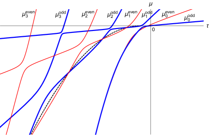
This definition produces a region in -plane and our goal is to determine the shape of this region (see Fig. 2) and to understand some of its properties. We have seen in [6] that the spectrum of the operator can be split into eigenvalue branches and depending on and an index and also depending on the evenness and oddness of the underlying eigenfunction. See details in [6] and Fig. 9. For each corresponding eigenvalue branch we will define two regions in -plane and then we will prove in Theorem 3 that those regions are the instability regions. That is, pairs in these regions are the length and tension parameters which give points in the Turing space, for the fixed reaction-diffusion parameter vector .
Definition \thedefinition (Instability region).
Fix a reaction-diffusion parameter vector that satisfies condition ((11)), and recall the number from ((9)), noting by ((11)). Define regions
for . If in addition satisfies condition ((13)) then the numbers and in ((10)) make sense, and we define
(The and notation refers to the sign of the unstable eigenvalues in the proof of Theorem 3 below.) Let and , for each .
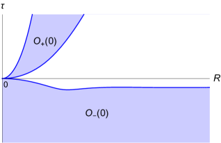
Fig. 1 shows the instability regions and associated to the zero-th even and odd eigenvalue branches, respectively. These figures were formed using implicit parameterizations of the eigenvalue branches and , respectively, as described at the end of the section.
In the next theorem, we will show that the instability regions we have found make up the whole Turing space . Remember that intersects both first and fourth quadrants in the -plane, while lies in the lower (fourth) quadrant, and similarly for and . Recall and .
Theorem 3 (Instability region associated to each eigenvalue branch).
In other words, if a pair belongs to the instability region or , , then Turing instability occurs for the domain with the tension parameter . That is, the spatially homogeneous linearly asymptotically stable steady state of ((7))–((8)) becomes unstable under diffusion.
We found infinitely many instability regions , in Theorem 3. We will discuss how these regions behave as increases in the following Proposition 3.
Proposition \theproposition (Movement of instability regions as index increases).
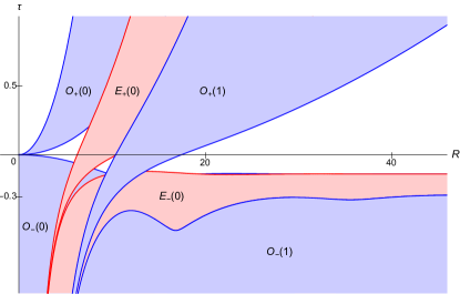
Fig. 2 shows some of these regions, and the nesting behavior.
Remark.
One might think it is obvious that we get Turing instability if because of existence of negative eigenvalues for . However, we show in the next corollary that having negative eigenvalue is not always enough to get instability. We have some region in the -plane with which corresponds to homogeneous steady states of the reaction-diffusion system staying stable. This stability relies upon a certain fact about the growth rate of the spectrum of with free boundary conditions when is small negative.
Corollary \thecorollary (Existence of region outside the Turing space).
Fig. 2 shows these regions. The corollary says there is some unshaded part in the lower half plane.
Extra instability regions when
In this subsection, we describe some additional instability regions when . From Theorem 1, there are two cases for the reaction-diffusion vector belonging to the Turing space when :
| either | ((11))–((13)) hold and , | ((16)) | ||
| or | ((17)) |
The instability regions and arise from the case ((17)), as shown in Definition 3 and Theorem 3. In addition to these regions shown in Fig. 2, in this subsection we will describe what the instability regions arising from the case ((16)) look like.
In the traditional Turing analysis with the Laplacian, the Turing space would be empty if ((14)) fails (that is, if ), because and are negative while the spectrum of the Laplacian is positive. But permits negative eigenvalues when . This introduces extra instability regions (as shown in Fig. 3), i.e., creates some Turing space.
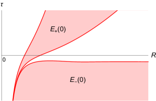
Assume the reaction-diffusion vector satisfies ((11))–((13)) and (meaning ((14)) fails). Define
Note that ((13)) guarantees the numbers and in ((10)) make sense, and these numbers are negative because . We present the regions and numerically in Fig. 3. The regions are obtained in a similar way to regions and . We use an implicit parameterization for and in terms of two other parameters [6, Theorem 11 and Lemma 13], but now we only need to consider eigenvalue branches in the lower half of the spectral plane.
Unlike the instability regions and in Definition 3 that only have upper boundary curves, the regions and have upper and lower boundary curves. To sum up, negative values introduce negative eigenvalues for the diffusion operator which lead to the appearance of some instability regions. These are relatively smaller than the regions and in Definition 3.
Numerical experiments.
We do some numerical simulations, to see beyond the linear predictions from spectral theory to what is happening in the genuinely nonlinear regime. We modify Gierer and Meinhardt’s reaction kinetics [9, Equation ], [16, Section ], to use the fourth order diffusion on the interval in -dimension. The Gierer–Meinhardt reaction system is
| ((18)) |
We fix constants for our numerical simulations. Hence the homogeneous steady state is
and the partial derivatives of and evaluated at the steady state are
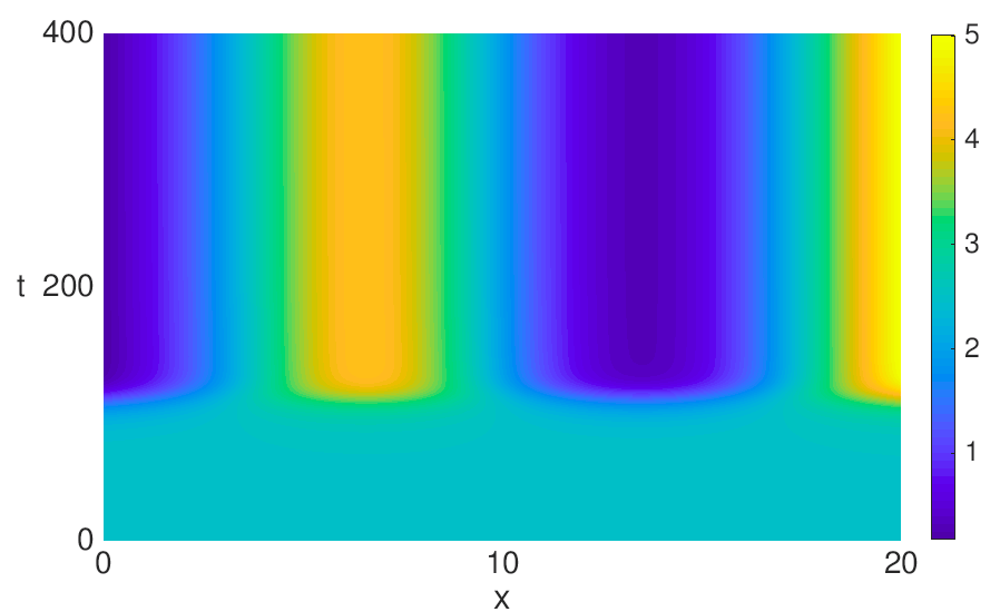
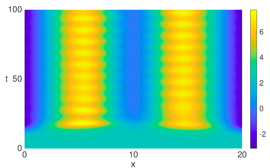
We also take the diffusivity . Figs. 4 and 5 illustrate inhomogeneous steady states corresponding to points in the instability regions and in Theorem 3 part (1). An unstable steady state for is illustrated in Fig. 4, which shows a slightly perturbed constant steady state evolving into a stripe pattern. The initial growth of the pattern takes place in the linear regime. The persistence of the pattern as it grows larger is due to the nonlinear effects (reaction). Fig. 5 illustrates an unstable steady state for . Again a perturbed steady state evolves into a stripe pattern. However, the experiment only gives patterns like Fig. 5 for about of random initial conditions. The rest of the simulations give irregular cycles of blow up, which might be due to numerical instabilities when .
Moreover, it is possible to get stability of the perturbed steady state when even though there is an unstable mode () in the linearized equation, as Corollary 3 shows. In about of our simulations (not shown), the initial perturbation decayed and the solution remained near the steady state until time , as predicted qualitatively by Corollary 3. In the other of simulations, the solution blew up chaotically, which again we think is due to numerical instabilities.
Plotting the instability regions
We end the section explaining how we create the instability regions in Figs. 1 and 2. For instance, the direct formula for the bottom boundary curve of the instability region is
from Definition 3. However, it is not straightforward to obtain the curve since we do not have have an explicit formula for as a function of . Instead we have the parameterized curves in terms of two other parameters [6, Theorem 5]. Hence, it is easy to work with a parameterized formula for Figs. 1 and 2:
where and are related by from [6, Lemma 2]. The point is that
and so by the parameterization in [6, Theorem 5] we see that equals the -value corresponding to the -value , which means
as we want.
The regions are special since each eigenvalue branch in the lower half of the spectral plane consists of infinitely many different parameterizations [6, Theorem 11 and Lemma 13], whereas regions are given by eigenvalue branches in the upper half of the spectral plane which consist of a single parameterization [6, Theorem 5]. So the boundary curves of and are made up with infinitely many parameterizations.
4. Proof of Theorem 1
Proof.
When we get the same conditions for Turing instability as when Laplacian diffusion is used [16, Section ], namely conditions ((11))–((14)). We give this proof below, since the later parts of the proof must be modified when .
Conditions ((11)) and ((12)) come from requiring linear stability of the ODE system in the absence of any spatial variation, as we now explain. Without spatial variation and satisfy
First, we linearize the system about the constant steady state : set , so that for small ,
where the derivative matrix is evaluated at . Look for solution of the form . The steady state is linearly stable if for each eigenvalue of the derivative matrix. That is, where satisfies the quadratic equation
Hence linearly stability of the constant steady state for the ODE system is guaranteed if ((11)) and ((12)) hold:
We assume these conditions throughout the rest of the proof.
Conditions ((13)) and ((14)) come from requiring linear instability of the PDEs (including the diffusion term) at the constant steady state, as we now explain. Consider the full reaction-diffusion system ((2))–((3)) and again linearize about to get
| ((23)) |
Define to be the time-independent solution of the eigenvalue problem:
with the free boundary conditions ((4))–((5)), where is the eigenvalue.
We look for a solution of ((23)) in the separated form
where ’s and ’s are constants. Note that the growth rate informs us about the stability of the homogeneous steady state with respect to the perturbation . If the real part of is negative for all , then any perturbations will tend to decay exponentially quickly. However, in the case that the real part of is positive for any value of , our expansion suggests that the amplitude of these modes will grow exponentially quickly and so the homogeneous steady state is linearly unstable. Substitution gives us for each ,
| ((24)) |
where is the diffusivity matrix and is the stability matrix. To get a nontrivial , formula ((24)) says must be an eigenvalue of the matrix , and so
Hence we get the eigenvalues as functions of the wavenumber , as the two roots of
| ((25)) | ||||
For the steady state to be unstable to spatial perturbation, we require
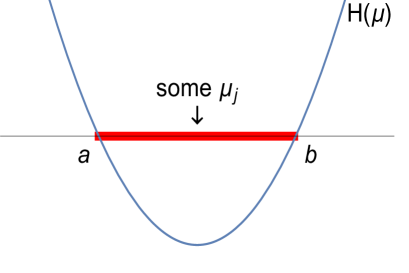
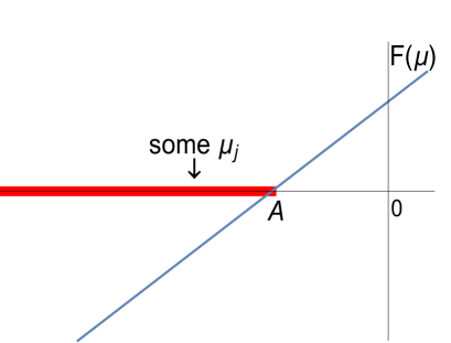
Recall that a quadratic equation with real coefficients has a root with positive real part if and only if either the sum of the roots is positive or the product of the roots is negative. Applied to the quadratic ((25)), that means we want or , for some . See Fig. 6.
Now, we will consider the cases and separately. When , the nd order “backwards” diffusion is ill-posed, meaning the nd order term destabilizes the system whereas the th order term stabilizes the system. In other words, two different types of diffusion compete when the tension parameter is negative. However, such competition does not happen in case. The th and nd order diffusion operators are each well-posed when . The case is very similar to the traditional Turing analysis with the Laplacian diffusion, since all eigenvalues of ((6)) are positive by the Rayleigh Quotient in Definition 2. On the other hand, the case is different from the traditional Turing instability since there are some negative eigenvalues.
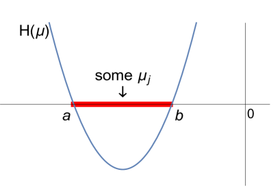
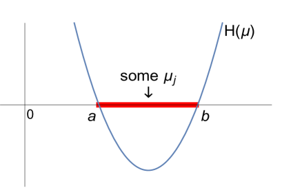
Case . When , the fact that is always positive (from Rayleigh Quotient in Definition 2) and from the stability condition ((11)) mean . So if and only if for some . See Fig. 7. Since by ((12)), we see if and only if ((13))–((14)) hold, meaning has distinct positive roots:
since for all . The first condition is a discriminant requirement. Hence, to be in Turing space, conditions – are necessary and sufficient, when ((11))–((12)) hold.
Case . Now, we will consider . The difference from comes from the fact that can be positive or negative and so both cases in Fig. 6 can happen in order to get . Therefore, to be in Turing space, either (which is hence ) or are necessary to hold.
For , must have distinct roots that have the same sign since the vertical intercept of the quadratic is by ((12)) and this gives a further necessary condition ((13)):
Also, the spectrum must intersect the interval :
where and are the distinct roots of , that is, the quantities defined in ((10)):
Note that we have two possibilities depending on the sign of (see Fig. 7). We do not have to satisfy because we are allowed to have negative wavenumber of . We have shown that when , in addition to conditions ((11))–((12)), either condition ((13)) and are necessary to hold, or else is necessary, for belonging to the Turing space.
Until now, we have showed necessary conditions to be in the Turing space, when . To finish proving the theorem, we have to show the conditions are sufficient. We show that belongs to the Turing space if
Assume first we are in situation of Fig. 6, meaning ((11))–((13)) hold and there exists at least one eigenvalue such that . Since , Turing instability occurs.
Assume now that we are in situation of Fig. 6, meaning ((11))–((12)) hold and
Since and so , Turing instability occurs. These prove the theorem when .
∎
5. Proof of Theorem 2 and Corollary 2
Proof of Theorem 2.
Step 1: Fix . We will prove the theorem first on a one-dimensional interval. Let ; an interval of length centered at the origin. We start by finding a rescaling relation. Let and . Then is defined on the interval . From the transformation, the differential equation ((6)) and the one-dimensional natural boundary conditions of the type ((4))–((5)) are converted into
and
Changing variable like this leads to the rescaling relation:
| ((26)) |
(We rescaled since we know from [6] how the eigenvalue behaves with respect to the parameter when the domain is fixed.)
Notice the following equivalent conditions, when is fixed:
| ((27)) |
where . There is at least one value and one index such that ((27)) holds, since we know from [6, Proposition ] there is at least one intersection between the eigenvalue curves for and the parabola . From the equivalent conditions, there is at least one value and one index such that
Hence . We have shown that
So
Letting shows .
Step 2: Extend to -dimensional cube in . Firstly we show extension to a -dimensional square domain. Let and . The first eigenvalue is the minimum of Rayleigh quotient over the space of all functions , by using the Rayleigh-Ritz variational formula, that is,
| ((28)) |
We can take a function of one variable in and regard it as a function of two variables, for instance, . Hence we obtain . By taking minimum of each Rayleigh quotient we get
where the second integral of the right side of ((28)) is cancelled because nothing depends on and so it comes down to the case of the first eigenvalue in one-dimensional domain. After taking infimum of and together with the above observation of one-dimensional case, we conclude that
It is straightforward to generalize -dimensional square case to -dimensional cubes.
∎
Proof of Corollary 2.
The point of Theorem 2 is that if then there exist domains that have arbitrarily negative value of . Hence the condition
in Theorem 1 holds for some domain . Together with the hypotheses that satisfies conditions ((11))–((12)), we conclude by Theorem 1 that Turing instability occurs for the domain . ∎
6. Proof of Theorem 3 and Proposition 3
Before we start the proof, we explain why we use the and notation for the sets and . For and in Definition 3, the eigenvalues and , which lie between positive constants by the condition ((14)), are positive. Hence, the sets and relate to eigenvalues that are in the upper half of the spectral plane. For and in Definition 3, the eigenvalues and are negative because they are less than the negative constant , by assumption ((11)). Hence, the sets and relate to eigenvalues that are in the lower half of the spectral plane.
Proof of Theorem 3.
-
(1)
“”: Pick one case as an example, since the other cases are similar. If conditions ((11))–((14)) on the reaction-diffusion vector are assumed, then we can apply Theorem 1 to show , as follows. Suppose , so that by Definition 3, the eigenvalue branch satisfies
Recall the domain is the interval . Together with the rescaling relation:
from ((26)), we have
Hence by Theorem 1, the reaction-diffusion vector belongs to the Turing space , and so . We have shown
“”: We will prove
in the following. Suppose , where . If , from Theorem 1, there exist some eigenvalue such that
From the analysis of the spectrum in [6] we know that eigenvalues correspond to some th branch of the spectrum (see Fig. 9). Note that from the condition ((14)) and so such are positive. Equivalently, there exist some th even or odd eigenvalue branches or such that
Together with the rescaling relation, it is equivalent to
Therefore, belongs to some instability regions or . The fact that is positive tells us is in the regions. We have shown that if with then
Now if , from Theorem 1, either there exists some eigenvalue such that
((29)) or else
((30)) The first case ((29)) is the same as we showed when . For the second case, recall from [6, Section ] that the first eigenvalue corresponds to the zero-th even or odd eigenvalue branch or (shown in Fig. 9). Note that from the condition ((11)) and so is negative. The second case ((30)) is equivalent to
From the rescaling relation,
Hence, belongs to the instability regions or . By combining when and the first and second cases of , we have shown
where recall , .
-
(2)
The proof is similar to part ((1)). “”, except using as the typical case instead of .
∎
Proof of Proposition 3.
-
(1)
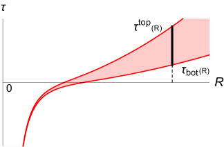
Fix and , and write . We will prove the even case and the odd case is similarly obtained. Define two sets from the definition of the instability region by the following:
Top ((31)) Bot ((32)) We will prove that these sets are graphs of functions of . First, we show that for given there is a single interval of -values that satisfies the condition
for being in the instability region in Definition 3. The condition is equivalent to
which is a single interval since is a strictly increasing function [6, Proposition ] so that the inverse is uniquely defined. See Fig. 8. Hence the sets ((31)) and ((32)) are the graphs of the function:
It is clear from Definition 3 that these are the top and bottom boundary curves of region .
Now, we will prove that moves downward as increases, in the sense that
Notice that for all ,
as proved in [6, Proposition ]. Since the eigenvalue branches are strictly increasing to infinity, we know that the inverse functions satisfy
for fixed . Therefore, we obtain
and similarly for the bottom curves.
-
(2)
Now we consider and , assuming conditions ((11))–((12)) hold. We will prove the even case and the odd case is similarly obtained. We will show the regions are nested as increases in the sense that the boundary curve of is nested as increases. We can express the boundary curve of as the function of in a similar way to part (1):
We will show that as increases,
For all , like above we have
and so
for fixed . Therefore, we obtain
∎
7. Proof of Corollary 3
.
To prove there exists stable region with , for each fixed satisfying ((11))–((14)), we study the region near the origin in Fig. 2. We will show:
| . The bottom boundary of lies above the horizontal axis . | ||
| . The boundary of lies below the horizontal axis . | ||
| . The boundary curves of , , and have as . |
Since the instability regions and move downwards as increases, by Proposition 3, there exist some regions near the origin that are not covered by any instability regions in .
Step : the bottom boundary of lies above the horizontal axis .
Recall the number from ((14)). Since is strictly increasing with [6, Proposition 7 and Section 3], we have . Hence,
which means the bottom boundary of lies above the horizontal axis .
Step : the boundary of lies below the horizontal axis .
We know from the spectrum, the eigenvalue branch is approximately a straight line near the origin [6, Section ]. Hence the boundary curve of satisfies
because by ((11)). Since the number is negative, the limit shows that the curve lies below some negative quadratic, near the origin.
Step : the boundary curves of , , and have as .
As , the limit of the upper boundary curve of is
since the inverse function from the spectrum of [6, Sections and ]. The same is true for , since .
As , the limit of the boundary curve of is
since the inverse function .
∎
8. Periodic boundary conditions in one dimension: Turing instability regions for the fourth order diffusion operator
In this section, we will illustrate the Turing instability region of the periodic boundary conditions, which has similar shape with the region for the free boundary conditions. The eigenvalue problem is
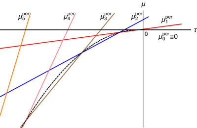
for . We can explicitly express the spectrum of periodic case in one dimension for as
where eigenfunctions can be taken as the even function or the odd function . Note that all the eigenvalues have multiplicity , except for . In the periodic case, we do not need to separate the even and odd instability regions since these regions are the same because eigenvalues associated to even and odd eigenfunctions are the same. We illustrate the spectrum in -plane, as shown in Fig. 10. Each branch is a straight line. We see there is a parabola on which the intersections of consecutive eigenvalue branches lie. The same parabola occurs also in the spectrum of the free boundary conditions as the parabola on which the intersections of the first even and odd eigenvalue branch and lie [6, Proposition ]. On top of that, we see the spectrum of periodic boundary conditions and the spectrum of free boundary conditions behave in asymptotically similar way: compare Fig. 10 and Fig. 9. Actual crossings occur in the spectrum of periodic boundary conditions, whereas there are barely-avoided crossings along eigenvalue branches for free boundary conditions. A pattern of barely-avoided crossings leads to a pattern of nearly-linear segments in the free case, while the periodic spectrum contains actual line segments. Similar spectral behavior of periodic and free boundary conditions should generate similar shape of the instability regions (Fig. 2 and Fig. 11).
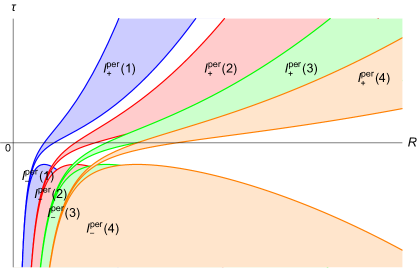
Assume conditions ((11))–((14)) hold on the reaction-diffusion vector . With a Turing analysis similar to Definition 3 and Theorem 3, we can express the instability region of periodic boundary conditions explicitly as follows, for the interval :
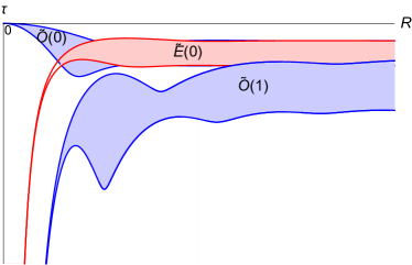
The instability regions of the first four eigenvalue branches of periodic case are illustrated in Fig. 11 in the -plane.
9. Acknowledgments
This research was supported by the University of Illinois Research Board (award RB17002).
References
- [1] S. Aly, I. Kim and D. Sheen. Turing instability for a ratio-dependent predator-prey model with diffusion. Appl. Math. Comput. 217 (2011) 7265–7281.
- [2] M. S. Ashbaugh, R. D. Benguria and R. Mahadevan. Minimization of the lowest eigenvalue of the vibrating clamped plate under compression. Forthcoming 2018.
- [3] A. L. Bertozzi, M. P. Brenner, T. F. Dupont and L. P. Kadanoff. Singularities and similarities in interface flows. Trends and perspectives in applied mathematics, Appl. Math. Sci., 100, Springer, New York (1994), pp. 155–208.
- [4] A. L. Bertozzi and M. C. Pugh. Long-wave instabilities and saturation in thin film equations. Comm. Pure Appl. Math. 51 (1998), no. 6, 625–661.
- [5] L. M. Chasman. An isoperimetric inequality for fundamental tones of free plates. Comm. Math. Phys. 303 (2011), no. 2, 421–449.
- [6] L. M. Chasman and J. Chung. Spectrum of the free rod under tension and compression. Appl. Anal., to appear (2018). doi:10.1080/00036811.2018.1451639
- [7] E. J. Crampin, E. A. Gaffney and P. K. Maini. Reaction and diffusion on growing domains: scenarios for robust pattern formation. Bull. Math. Biol. 61(6) (1999), 1093–1120.
- [8] R. Dillon, P. K. Maini and H. G. Othmer. Pattern formation in generalized Turing systems. I. Steady-state patterns in systems with mixed boundary conditions. J. Math. Biol. 32 (1994), no. 4, 345–393.
- [9] A. Gierer and H. Meinhardt. A theory of biological pattern formation. Biol. Cybern (1972). 12, 30–39.
- [10] V. Klika and E. A. Gaffney. History dependence and the continuum approximation breakdown: the impact of domain growth on Turing’s instability. Proc. A. 473 (2017), no. 2199, 20160744, 19 pp.
- [11] J. M. Lee, T. Hillen and M. A. Lewis. Pattern formation in prey-taxis systems. J. Biol. Dyn. 3 (2009), no. 6, 551–573.
- [12] M. A. Lewis. Spatial coupling of plant and herbivore dynamics: the contribution of herbivore dispersal to transient and persistent “waves” of damage. Theor. Popul. Biol. 45 (1994), 277–312.
- [13] M. A. Lewis, P. K. Maini and S. Petrovskii. Dispersal, Individual Movement and Spatial Ecology: A Mathematical Perspective. Lecture Notes in Mathematics, 2071. Springer, Heidelberg, 2013.
- [14] A. Madzvamuse, E. A. Gaffney and P. K. Maini. Stability analysis of non-autonomous reaction-diffusion systems: the effects of growing domains. J. Math. Biol. 61 (2010), no. 1, 133–164.
- [15] P. K. Maini, T. E. Woolley, R. E. Baker, E. A. Gaffney and S. S. Lee. Turing’s model for biological pattern formation and the robustness problem. Interface Focus 2, 487 (2012).
- [16] J. D. Murray. Mathematical biology. II. Spatial models and biomedical applications. Third edition. Interdisciplinary Applied Mathematics, 18. Springer-Verlag, New York, 2003.
- [17] M. Neubert, M. Kot and M. A. Lewis. Dispersal and pattern formation in a discrete-time predator-prey model. Theoretical Population Biogy, 48(1) (1995): 7–43.
- [18] H. F. Nijhout, P. K. Maini, A. Madzvamuse, A. J. Wathen and T. Sekimura. Pigmentation pattern formation in butterflies: experiments and models. Comptes Rendus Biologies 2003; 326(8): 717–727. PMID: 14608692
- [19] R. G. Plaza, F. Snchez-Garduo, P. Padilla, R. A. Barrio and P. K. Maini. The effect of growth and curvature on pattern formation. J. Dynam. Differential Equations 16 (2004), no. 4, 1093–1121.
- [20] J. A. Sherratt, B. T. Eagan and M. A. Lewis. Oscillations and chaos behind predator-prey invasion: mathematical artifact or ecological reality? Philos Trans. R. Soc. London Ser. B 352 (1997) 21–38.
- [21] G. Sweers. On sign preservation for clotheslines, curtain rods, elastic membranes and thin plates. Jahresber. Dtsch. Math.-Ver. 118 (2016), no. 4, 275–320.
- [22] A. M. Turing. The chemical basis of morphogenesis. Philos. Trans. Roy. Soc. London Ser. B 237 (1952), no. 641, 37–72.