Neural Random Projections for Language Modelling

Abstract

Neural network-based language models deal with data sparsity problems by mapping the large discrete space of words into a smaller continuous space of real-valued vectors. By learning distributed vector representations for words, each training sample informs the neural network model about a combinatorial number of other patterns. In this paper, we exploit the sparsity in natural language even further by encoding each unique input word using a fixed sparse random representation. These sparse codes are then projected onto a smaller embedding space which allows for the encoding of word occurrences from a possibly unknown vocabulary, along with the creation of more compact language models using a reduced number of parameters. We investigate the properties of our encoding mechanism empirically, by evaluating its performance on the widely used Penn Treebank corpus. We show that guaranteeing approximately equidistant (nearly orthogonal) vector representations for unique discrete inputs is enough to provide the neural network model with enough information to learn –and make use– of distributed representations for these inputs.

neural networks, random projections, online learning, distributional semantics, natural language processing, semantics, computational semantics, language modelling

1 Introduction

The goal of computational semantics is to automate the learning of meaningful representations for natural language expressions. In particular, representation learning is integral to state-of-the-art Language Modelling (LM), which is a keystone in computational semantics used for a wide range of Natural Language Processing (NLP)tasks, from information retrieval (Ponte & Croft, 1998) to speech recognition (Arisoy et al., 2012), or machine translation (Koehn, 2010). Better language models frequently lead to improved performance on underlying downstream tasks, which makes LM valuable in itself. Moreover, certain domains allow language models to extract knowledge implicitly encoded in the training data. For example, in (Serban et al., 2016), learning from film subtitles allows models to answer basic questions about colours and people. Learning representations for discrete symbols is particularly useful in the context of language models because capturing regularities in relationships between words (which are not only complex but recursive in nature) allows us to build better models. The LM, as a task, can thus be seen as a framework for the study of more general learning approaches operating in fairly complex and sometimes dynamic scenarios.

The goal of LM is to model the joint probability distribution of words in a text corpus. Models are trained by maximising the probability of a word given all the previous words in the training dataset, formally:

$$P(w_{1},\ldots,w_{N})=\prod_{i=1}^{N}P(w_{i}|h_{i}),$$

where $w_{i}$ is the current word and $c_{i}=(w_{1},\cdots,w_{i-1})$ is the current word history or context. A Markov assumption is usually used as approximation: instead of using the full word history as context, the probability of observing the $i^{th}$ word $w_{i}$ is approximated by the probability of observing it in a shortened context of $n-1$ preceding words. To train a language model under this assumption, a sliding window $(w_{i},c_{i})$ of size $n$ is applied sequentially across the textual data. Each window is also commonly referred to as n-gram.

Traditional n-gram models (Brown et al., 1992; Kneser & Ney, 1995) are learned by building conditional probability tables for each $P(w_{i}|c_{i})$. This approach is popular due to its simplicity and overall good performance, but this formulation poses some obstacles. More specifically, we can see that even with large training corpora, extremely small or zero probabilities can be given to valid sequences, mostly due to rare word occurrences. Dealing with this sparseness and unseen data requires smoothing techniques that reallocate probability mass from observed to unobserved n-grams, producing better estimates for unseen data (Kneser & Ney, 1995). The fundamental issue is that classic n-gram models lack a notion of word similarity. Words are treated as equality likely to occur discrete entities with no relation to each other. This makes density estimation inherently difficult, as there is no straightforward way to perform smoothing. As an example, there is no way to estimate the probability for two sequences differing only in a synonymic expression.

Neural networks have been used as a way to deal with both the sparseness and smoothing problems. The work in (Bengio et al., 2003) represents a paradigm shift for language modelling and an example of what we call Neural Network Language Models (NNLM). In a NNLM, the probability distribution for a word given its context is modelled as a smooth function of learned real-valued vector representations for each word in that context. The neural network models learn a conditional probability function $P(w_{i}|c_{i};\theta_{F},\theta_{L})$, where $\theta_{F}$ is a set of parameters representing the vector representations for each word and $\theta_{L}$ parameterises the log-probabilities of each word based on those learned features. A softmax function is then applied to these log-probabilities to produce a categorical probability distribution over the next word given its context. (In section 3, we will present two instances of neural network models following this formulation.)

The resulting probability estimates are smooth functions of the continuous word vector representations, and so, a small change in such vector representations results in a small change in the probability estimation. Smoothing is learned implicitly, leading NNLM to achieve better generalisation for unseen contexts. The resulting word vector representations are also commonly referred to as embeddings, since they represent a mapping from the large discrete space (a vocabulary) to a smaller continuous space of real-valued vectors where they are “embedded”. This constitutes a geometric analogy for meaning with the that, with proper training, words that are semantically or grammatically related will be mapped to similar locations in the continuous space.

Energy-based models provide a different perspective on statistical language modelling with parametric neural networks as a way to estimate joint discrete probability densities. Energy-based models such as (Mnih & Hinton, 2007; Mnih et al., 2009) capture dependencies between variables by associating a scalar energy score to each variable configuration. In this case, making predictions consists on setting the values for observed or visible variables and finding the value for the remaining (hidden) variables that minimise this energy score.

The key difference between the energy-based models in (Mnih & Hinton, 2007; Mnih et al., 2009) and the NNLM in (Bengio et al., 2003) is that instead of estimating a categorical distribution based on higher-level features produced by the NNLM hidden layer based on the distributed representations for the context words, an energy-based model tries to predict the distributed representation of a target word and attributes an energy score to the output configuration of the model based on how close the prediction is from the actual representation for the target word. The correct representation for the target word is dependent on the current state of the model embedding parameters, but two separate parameter matrices can also be used for context and target words (Mnih & Teh, 2012). Most probabilistic models can in fact be viewed as a special type of energy-based model in which the energy function has to satisfy certain normalisation conditions, along with a loss function with a particular form. Moreover, energy-based learning provides a unified framework for learning, and can be seen as an alternative to probabilistic estimation for prediction or classification tasks (Lecun et al., 2006).

In this paper, we describe an encoding mechanism that can be used with neural network probabilistic language models to represent unique discrete inputs while using a reduced parameter space. Our models use random projections as a way to encode input patterns, using a fixed size sparse random vector. The idea is to maintain the expressive power of the neural networks while reducing the parameter space and expanding the types of discrete patterns the network can use to make predictions. Following the principles from (Achlioptas, 2003) and (Kanerva, 2009), our random projection encoding reduces the input dimension $|V|$ to a lower $k\text{-dimensional}$ dimensional space while approximately preserving the distances between expected input patterns. This means that instead of using the $1\text{-of-}V$ orthogonal encoding, we use a fixed $k\text{-dimensional}$ sparse vector with each input word being nearly-orthogonal to any other words. Our main hypothesis is that in order for a neural network to learn distributed representations for words, we do not require one unique vector representation per word; instead, we just need the representations of each pair of unique patterns to be approximately orthogonal. Each unique pattern should (by itself) be indistinguishable from any other unique pattern. By using random projections, we guarantee that each new representation is equally probable and nearly-orthogonal to any other representation. This encapsulates the idea that what makes a word unique in language is not its representation, but the way in which we use the word, since language is essentially a system of differences, where meaning in words arises through social social interaction (Feyerabend, 1955), and biological biases (Pinker, 2010).

2 Background and Related Work

In this paper, the goal is two fold: to reduce the dimensionality of the input space, and to allow neural-network models to capture patterns that are usually intractable to represent using the typical count-based n-gram models. In the case of neural language modelling, each word is usually represented by a $1\text{-of-}V$ vector. The input space is an orthogonal unit matrix where each word is represented by a single value $1$ on the column corresponding to its index. This means that if we want to represent a more complex structured space such as syntactic dependency trees, this would require either to use structured neural network (Socher et al., 2011), or to index all possible unique combinations of syntactic structures which is intractable for large datasets. This article is a first step in the exploration the possibility of encoding complex structured discrete spaces. We take an incremental and bottom-up approach to the problem by exploring how to build an encoder that can be used in word-level language models.

One cornerstone of neural-network-based models is the notion of distributed representation. This is, the fact that neural network can learn vector representations for discrete inputs as weights that are learned during the training process. In a distributed representation, each ”thing” is represented as a combination of multiple factors. Learning distributed representations of concepts as patterns of activity in a neural network has been object of study in (Hinton, 1986). The mapping between unique concept ids and respective vector representations has been later referred to as embeddings. The idea of using embeddings in language modelling is explored in the early work or Bengio et al. (Bengio et al., 2003) and later popularised by the word2vec method for word representation learning (Mikolov et al., 2013b). Both these methods encode input words using a $1\text{-of-}V$ encoding scheme, where each word is represented by its unique index. The size of the embedding space is thus proportional to the size of the vocabulary.

In the case of language modelling, there have been multiple developments to deal with large or unknown vocabularies. One straightforward method is to consider character or subword-level (e.g. morphemes) modelling instead of considering words the discrete input units (Ling & Dyer, 2015; Kim et al., 2016; Zhang & LeCun, 2015). The main motivation behind using subword-based modelling is that training accurate character-level models is extremely difficult and often more computationally expensive than working with models that use word-level inputs (Mikolov et al., 2012), but Elman shows that most of the entropy if concentrated at the first few characters of each word (Elman, 1990). Moreover, word-based models often fail to capture regularities in many inflectional and agglutinative languages. In this paper we focus on word-based modelling but the proposed encoding mechanism can be incorporated in models that use morphemes instead of words as inputs.

Despite the good results obtained with word-level neural probabilistic language models (Bengio et al., 2003; Mnih & Hinton, 2007), these have notoriously long training times, even for moderately-sized datasets. This is due to the fact that in order for these models to output probability distributions, they require explicit normalisation, which requires us to consider all words in the vocabulary to compute log-likelihood gradients. Solutions to this problem include structuring the vocabulary into a tree, which speeds up word probability computations –but ties model predictive performance to the tree used (Morin & Bengio, 2005). Another approach is to use a sampling approach to approximate gradient computations. In particular, Noise Constrastive Estimation (NCE)(Gutmann & Hyvärinen, 2012) has been shown to be a stable approach to speed up unnormalised language models (Mnih & Teh, 2012). While we use full normalisation to analyse the predictive capability of our proposed models, much like in the previous case, the computational complexity introduced by the normalisation requirements can be alleviated using techniques like NCE. Nevertheless, using random projections to model unique discrete inputs with neural networks, changes the dynamics of the language modelling problem. This warrants an assessment of how effective approximation methods are –which we will do in future work.

Exploiting low-dimensional structure in high-dimensional problems has become a highly active area of research in machine learning, signal processing, and statistics. In summary, the goal is to use a low-dimensional model of relevant data in order to achieve, better prediction, compression, or estimation compared to more complex ”black-box” approaches to deal with high-dimensional spaces (Hegde et al., 2016). In particular, we are interested in the compression aspect of these approaches. Usually, exploiting low-dimensional structure comes at a cost, which is the fact that incorporating structural constraints into a statistical estimation procedure often results in a challenging algorithmic problem. Neural network models have been notoriously successful at dealing with these kind of constraints, and even at finding geometric analogies for complex patterns such as syntactic relationships (Mikolov et al., 2013a). But the use of neural networks has been limited in the types of patterns that it can process and encode. Particularly, there is no straightforward way to encode priors about discrete input qualifiers or to encode structure within the input space –although some work has been done in that direction (Vaswani et al., 2017).

In this article we show that neural network models can be used to tackle a challenging statistical estimation problem such as language modelling, while using an approximation method to encode a large number of discrete inputs –and possibly allowing for the additional encoding of linguistic-based structural constraints. To achieve this, we turn to a simple yet efficient class of dimensionality reduction methods, random projections.

The use of random projections as a dimensionality reduction tool has been extensively studied before, especially in the context of approximate matrix factorisation –the reader can refer to (Halko et al., 2011) for a more in depth review of this technique. The basic idea of random projections as dimensionality reduction technique comes from the work of Johnson and Lindenstrauss, in which it was shown that the pairwise distances among a collection of $N$ points in an Euclidean space are approximately maintained when the points are mapped randomly to an Euclidean space of dimension $O(\log N)$. In other words, random embeddings preserve Euclidean geometry (Johnson & Lindenstrauss, 1984). In the case of language modelling, we assume that finding representations for words is a problem of geometric nature (see (Levy et al., 2014)) that can be translated to a lower-dimensional space and solved there.

Random projections have been used in multiple machine learning problems as a way to speed-up computationally expensive methods. One example is the use of random mappings for fast approximate nearest-neighbour search (Indyk, 2001). Random projections have also been applied to document retrieval or representation learning based on matrix factorisation. In (Papadimitriou et al., 1998), random projections are used as a first step for Latent Semantic Analysis (LSA), which is essentially a matrix factorisation of word co-occurrence counts (Landauer & Dumais, 1997). This makes the matrix factorisation algorithm much more tractable, because the projections preserve pair-wise distances used by the algorithm to find latent vector representations for documents – representations that explain word frequency variance well. A similar approach is followed in (Kaski, 1998): a random mapping projection is applied to document vectors to reduce their dimensionality; these vectors then serve as input to a Self-Organising Map (SOM)in order to cluster the documents according to their similarity. This approach was motivated by experiments from (Ritter & Kohonen, 1989), where instead of performing document clustering based on word co-occurrence frequencies, the authors performed word clustering after reducing the context vector dimensionality using random projections. In the later work of Kanerva, an incremental random projection method called random indexing, is used to gather co-occurrence patters in an incremental fashion (Kanerva et al., 2000). This was motivated by previous work on associative memory models (Kanerva, 1988), and the work in (Achlioptas, 2003), which showed that a random projection matrix can be constructed incrementally using a simple sparse ternary distribution (while still respecting the bound-preserving requirements from the Johnson and Lindenstrauss lemma (Johnson & Lindenstrauss, 1984)).

Our proposal of using random projections as the encoding mechanism for neural network language models is also related to dictionary learning. Dictionary learning consists of modelling signals as sparse linear combinations of atoms selected from a learned dictionary (Gribonval et al., 2015).

In this paper, we focus on exploring simple feedforward neural network architectures for multiple reasons. First, using incrementally complex models allows us to determine which architectural components allow neural network models to deal with random-projection encoding. The work from Mnih et al. in energy-based neural language models (Mnih & Hinton, 2007; Mnih et al., 2009) is a good starting point for our baseline because the energy-based model gives us a way to translate random vector predictions into word probability distributions.

Recurrent architectures have been successfully used in language modelling and related tasks (Jozefowicz et al., 2016) –with these successes often being attributed to their capacity (in principle) to capture unbound contexts (retaining long term dependencies and ensuring that information can be propagated through many time steps). We remain cautious about their use –as a baseline– for our proposed approach. In practice, it is not clear whether or not the capacity to capture long-term dependencies (in principle) is key to achieve good results in all tasks related to LM. For example, neural networks with a simple architecture and convolution operations, capable of dealing with fixed contexts, have been proposed as a competitive alternative to Long Short Term Memory (LSTM)networks (Dauphin et al., 2016). As another example, good performance can be achieve in a translation task by using attention mechanism with a feedforward architecture (Vaswani et al., 2017).

Most importantly, using over-parametrised/complex architectures undermines our ability to distinguish between a model that performs well with a new component, and a model that performs well despite the new component. We do intend to explore the proposed encoding with recurrent architectures in the future, but for now, this is beyond the scope of this paper.

3 NRP Model

In this section, we describe our neural random projection approach to language modelling. The main idea is to use a neural network model to learn lower-dimensional representations for discrete inputs while learning a discrete probability distribution of words similarly to (Bengio et al., 2003; Mnih & Hinton, 2007). By contrast with the existing work, instead of encoding a word using a $1\text{-of-}V$ vector, each word is encoded using a random sparse high-dimensional vector (Kanerva et al., 2000; Kanerva, 2009). This allows us to create neural-network models with a smaller number of parameters, but crucially, it also allows for more flexible patterns to be represented and for a model to be trained with a vocabulary of unknown size.

3.1 Random Input Encoding

The distributed representations or embeddings in our model are $k\times m$ subspace, with $k<<|V|$ (we have less base vectors than words in the known dictionary). A representation for each word as learned by the neural network is the linear combination of $(s\times m)\text{-dimensional}$ basis where $s$ is the number of non-zero entries for each vector. Each unique word is assigned a randomly generated sparse ternary vector we refer to as random index vector. Random indices are sampled from the following distribution with mean $0$ and variance $1$:

$$r_{i}=\left\{\begin{array}[]{rl}+1&\mbox{with probability }\alpha/2\\ 0&\mbox{with probability }1-\alpha\\ -1&\mbox{with probability }\alpha/2\end{array}\right.$$ (1)

where $\alpha$ is the proportion of non-zero entries in the random index vector. While similar to the distribution proposed in (Achlioptas, 2003), we use very sparse random vectors and no scaling factor. Since the input space is an orthogonal unit matrix, the inner product between any two random vectors $(r_{i},r_{j})$ is expected to be concentrated at $0$. The motivation for this is to make any discrete input indistinguishable from any other input in terms of distance between them. Instead of referring the sparseness parameter $a$, we will use $s$ as the number of non-zero entries for randomly generated index vectors. This means that for $s=2$ we have exactly one entry with value $1$, one with value $-1$ and all the rest have value $0$.

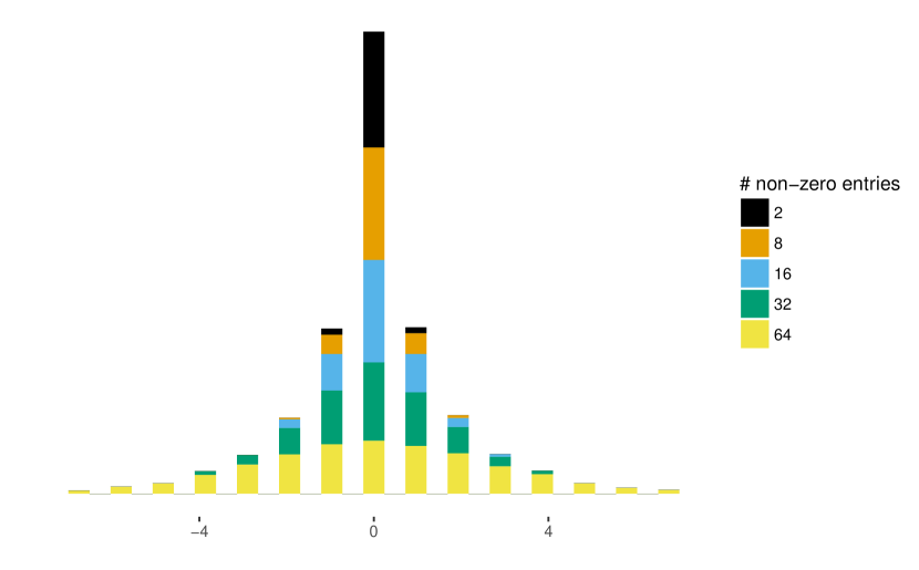
Figure 1: Distribution of inner products between pairs of randomly generated 1000-dimensional random indices.

Figure 1 shows the distribution of inner products for a $1000-k$ dimensional random indices. A larger number of non-zero entries leads to a greater probability of a collision to occur, but the inner products remain well concentrated at $0$ – any two random sparse vectors are expected to be either orthogonal or near orthogonal.

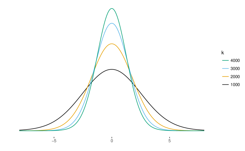
(a) Ternary random indices

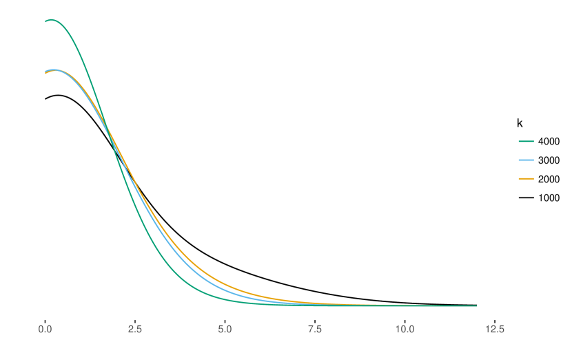
(b) Binary random indices

Figure 2: Inner product distribution for different values of random index dimension $k$, aggregating the distributions for multiple numbers of non-zero entries. Ternary random indices 2(a) have entries with values $\in\{-1,0,1\}$, while binary random indices have entries with values $\in\{0,1\}$.

Having more non-zero entries adds to the proabability of having collisions (same columns between two vectors having non-zero values), which leads to larger inner products, nevertheless the inner product distribution does not deviate much from $0$. We will see later that having random mappings with more non-zero entries is not necessarily bad as it adds to the robustness of the input encoding – making it easier for the neural network model to distinguish between different input patters despite the collisions.

If we take the distributions in figure 1 as a profile for inner product concentration for a random index with dimension $k$ (in this case 1000), and we vary this $k$. We can see how the inner product becomes more concentrated on $0$ for higher dimensional random indices (figure 2). In section 4 we will show how different sizes of random indices and number of non-zero entries affect the predictive capabilities of our neural network language models. One of the goals is to figure out if neural networks can still make predictions based on a compressed signal of its input, and to figure out if adding more non-zero entries (increasing the probability of collisions) hurts performance. Another question we explore is the importance (or irrelevance) of using binary (figure 2(b)) vs ternary (figure 2(a)) random indices.

3.2 Baseline Model Architecture

In order to assess the performance of our added random projection module, we build a baseline model without random projections. The architecture for this model is based in the one in (Bengio et al., 2003) but instead of predicting the probability of each word directly we use the energy-based definition from Mnih’s work (Mnih & Hinton, 2007). The baseline model learns to predict the feature vector (embedding) for a target word along with a probability distribution for all the known words conditioned on the learned feature vectors of the input context words. Figure 3 shows an overview of our baseline model.

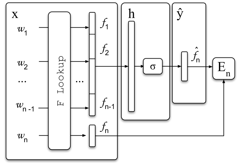
Figure 3: Baseline feedforward energy model based on (Bengio et al., 2003; Mnih & Hinton, 2007).

The baseline language model in figure 3 converts each word into a vector of real-valued features using a feature lookup table $F$. The goal is to learn a set of feature vectors in $F$ that are good at predicting the feature vector for the target word $w_{n}$. Each word in a context of size $n-1$ is converted to $n-1$ $m\text{-dimensional}$ feature vectors that are then concatenated into a $(n-1)\times m$ vector and passed to the next layer $h$ that applies a non-linear transformation:

$$h_{j}=\sigma\left(W_{h}f+b_{h}\right)$$ (2)

where $f$ is a vector of $n-1$ concatenated feature vectors, $b$ is a bias for the layer $h$ and $\sigma$ is a non-linear transformation (e.g. sigmoid, hyperbolic tangent, or rectifier linear unit (ReLU)). We found ReLU units (equation 3) to perform well and at an increased training speed, so we use this transformation in our models.

$$f(x)=max(0,x)$$ (3)

The result of the non-linear transformation in $h$ is then passed to a linear layer $\hat{y}$ that predicts the feature vector $\hat{f}_{n}$ for the target word $w_{n}$ as follows:

$$\hat{y}_{n}=W_{\hat{y}}h+b_{\hat{y}}$$ (4)

The energy function $E$ is defined as the dot product between the predicted feature vector $\hat{f}_{n}$, and the actual current feature vector for the target word $f_{n}$:

$$E_{n}=\hat{f}^{T}_{n}f_{n}$$ (5)

To obtain a word probability distribution in the network output, the predicted feature vector is compared to the feature vectors of all the words in the known dictionary by computing the energy value (equation 5) for each word. This results in a set of similarity scores which are exponentiated and normalised to obtain the predicted distribution for the next word:

$$P(w_{n}|w_{1}:n-1)=\frac{\exp(E_{n})}{\sum_{j}^{|V|}\exp(E_{j})}$$ (6)

The normalisation factor is the sum of the energy values for all the words in the dictionary. Contrary to the work in (Mnih et al., 2009), we didn’t find any advantage in adding bias values based on the frequencies of the known words in the dictionary, so we use a pure energy-based definition.

The described baseline model can be though of as the standard feedforward one, as defined in (Bengio et al., 2003) with an added linear layer $\hat{y}$ of the same size as the embedding dimensions $m$. Furthermore, instead of using two different sets of embeddings to encode context words and compute the word probability distributions, we learn a single set of feature vectors $F$ that are shared between input and output layers to compute the energy values and consequently the probability distribution over words.

3.3 NRP Model Architecture

We incorporate our random projection encoding into the previously defined energy-based neural network language model following the formulation in (Mnih & Hinton, 2007; Mnih et al., 2009). We chose this formulation because it allows us to use maximum-likelihood training and evaluate our contribution in terms of perplexity. This makes it easier to compare it to other approaches that use the same intrinsic measure of model performance. It is well known that computing the normalisation constant (the denominator in equation 6) is expensive, but we are working with relatively simple models, so we compute this anyway. It should be noted that the random projection definition is compatible with much more economical approximation methods such as Noise Constrastive Estimation (NCE)(Mnih & Teh, 2012), and as such, we plan to test this method in the future along with other evaluation methods.

Having defined the baseline model, we now extend it with a random projection lookup layer. The overview of the resulting architecture can be seen in figure 4.

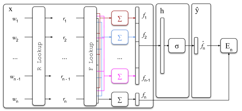
Figure 4: Neural random projection feedforward energy model.

There are two major differences between this and the previous model. First of all, we include a random index lookup table that generates a new random index for each new word that it encounters. Tho get the feature representation for a given word $w_{i}$ we multiply its $k-\text{dimensional}$ random index by the $k\times m$ feature matrix $F$. The resulting vector representation for a word $w_{i}$ is given by the sum of all the feature vectors extracted for each non-zero entry in the random index. Much like in existing models, only the rows corresponding to the non-zero entries are modified during training for each input sample. This adds to the computational complexity of the first layer since we are no longer selecting a single feature vector for each word, but it is still quite efficient ,since for $n-1$ words in a context, the feature vectors for the context can be retrieved as single sparse multiplication.

The second difference is that to compute the output probability normalisation constant, we can no longer compute the dot product between the predicted feature vector $\hat{f}_{n}$ and the feature matrix $F$ as $\hat{f}_{n}^{T}F$ because we no longer have one per word. Instead, we must first find the feature vectors for all the words by multiplying all the random indexes for all the words stored in the random index lookup $R$ by $F$ as $F^{\prime}=R^{T}R$ and then find the normalisation constant by computing the dot product between the predicted feature vector and $F^{\prime}$. The probability normalisation function is thus given by:

$$\sum_{j}^{|V|}\exp(\hat{f}_{j}^{T}r_{j}),$$ (7)

where $r_{j}$ (as we can see in figure 4) is the sparse random index for word $w_{j}$. While all these operations can be implemented using sparse matrix multiplications, the computational complexity of each training or inference step scales linearly with the number of non-zero entries in the random indices $s$. As we stated previously, techniques like NCE,can alleviate the problem since the issue lies in the fact that we need to compute the partition term to learn an output probability distribution.

The fact that we can learn features for a vocabulary incrementally does not eliminate the fact that we need to compute the normalisation constant or the fact that the model does not deal with out-of-vocabulary words. Nevertheless, we are adding to neural network models, is the possibility of building predictive models based on a compression of the input space and enabling the possibility for the encoding of more complex (and possibly structured) inputs using random projections similarly to (Basile et al., 2011).

Since all models output probability distributions, they are trained using a maximum likelihood criterion:

$$\mathcal{L}=\frac{1}{T}\sum_{t}\log P(w_{t},w_{t}-1,\ldots,w_{t}-n+1;\theta)$$ (8)

Where $\theta$ is the set of parameters learned by the neural network in order to maximise a corpus likelihood.

In the following section, we present our experimental setup. We start by describing the used dataset, evaluation metrics, along with a brief description of the hyper-parameters found in exploratory model fine-tuning. We proceed to show how random index encoding influences model performance and compare the model with the previously described baseline.

4 Experimental Results

4.1 Experimental Setup

We evaluate our models using a subset of the Penn Treebank corpus, more specifically, the portion containing articles from the Wall Street Journal (Marcus et al., 1993). We use a commonly used set-up for this corpus, with pre-processing as in (Mikolov et al., 2011) or (Kim et al., 2016), resulting in a corpus with approximately 1 million tokens (words) and a vocabulary of size $|V|=10\text{K}$ unique words The dataset is divided as follows: sections 0-20 were used as training data ($930$K tokens), sections 21-22 as validation data (74K tokens) and 23-24 as test data ($82$K tokens). All words outside the 10K vocabulary were mapped to a single token $<unk>$. We train the models by dividing the PTB corpus into n-gram samples (sliding windows) of size $n$. All the models here reported were $5-text{g-ram}$ models. To speed up training and evaluation, we batch the samples in mini-batches of size $128$ and the training set is randomised prior to batching.

We train the models by using the cross entropy loss function. Cross entropy measures the efficiency of the optimal encoding for the approximating (model predicted) distribution $q$ under the true (data) distribution $p$:

$$H(p,q)=-\sum_{x}p(x)log(q(x))$$ (9)

We evaluate and compare the models based on their perplexity:

$$\text{PPL}=\exp\left(-\frac{1}{N}\sum_{w_{1:n}}logP(w_{n}|w_{1:n-1})\right)$$ (10)

where the sum is performed over all the n-gram windows of size $n$. Another way to formulate perplexity is as follows:

$$2^{H(p,q)}=2^{-\sum_{x}p(x)log(q(x))}$$ (11)

Perplexity is essentially a geometric average of inverse probabilities; it measures the predictability of some distributions, given the number of possible outcomes of an equally (un)predictable distribution, if each of those outcomes was given the same probability. (Example: if a distribution has perplexity $6$, it is as unpredictable as a fair dice. Since all the models are trained using mini-batches, all perplexities are model perplexities, this is, the average perplexity for all the batches.)

Along with model performance, we also report the approximate number of trainable parameters of each model configuration which can be computed as:

$$\#p=(|x|\times m)+((m\times(n-1))\times h+h)+(h\times m+m)$$

where $|x|$ s the dimension of input vectors, $m$ is the dimension of the feature lookup layer (or embeddings), $n$ is the n-gram size (in this case $5$), and $h$ is the number of hidden units.

We train our models using Stochastic Gradient Descent (SGD)without momentum. In early experiments, we found that SGD produced overall better models and generalised better than adaptive optimisation procedures such as ADAM (Kingma & Ba, 2014). Model selection and early stopping is based on the perplexity measured on the validation set.

We used a step-wise learning rate annealing ,where the learning rate is kept fixed during a single epoch, but we shrink it by $0.5$ every time the validation perplexity increases at the end of a training epoch. If the validation perplexity does not improve, we keep repeating the process until a given number of epochs have passed without improvement (early stop). The patience parameter (number of epochs without improvement before stopping) is set to $3$ and it resets if we find a lower validation perplexity at the end of an epoch. We consider that the model converges when it stops improving and the patience parameter reaches $0$

As for regularisation, dropout (Srivastava et al., 2014) and $\ell^{2}$ weight penalty performed similarly. We opted for using dropout regularisation in all the models. Dropout is applied to all weights including the feature lookup (embeddings). In early experiments, we used a small dropout probability of $0.05$ following the methodology in (Pham et al., 2016) (where the authors use smaller dropout probabilities due to the Penn Treebank corpus being smaller. We later found that,dropout probabilities interact non-linearly with other architectural parameters such as embedding size and number of hidden units. Higher dropout probability values can be used (and give us better models) in conjunction with larger embedding and hidden layer sizes.

We found that Rectifying Linear Units (ReLU) activation units (He et al., 2015) performed better than saturating non-linear functions like hyperbolic tangent, or alternatives like Exponential Linear Units (ELUs) (Clevert et al., 2015). Figure 5 shows the distribution of test perplexity for models using random projections with different activation functions on the non-linear projection layer. Overall, ELUs are the most sensitive to larger dropout regularisation and didn’t produce significantly better results than the models using the hyperbolic tangent. Rectifier linear units seem to outperform other types of non-linearities both in our baseline and the models using random projections (NRP).

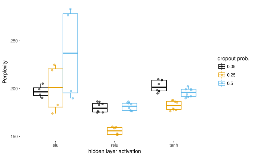
Figure 5: Average test perplexity of best NRP models for different hidden activation functions for a feature lookup size (embeddings) $m=128$, a number of hidden units $h=256$, random indices of dimension $k=5000$ and number of non-zero units $s=8$

One problem encountered when using ReLU units was that they caused gradient values to explode easily during training. To mitigate this, we added local gradient norm clipping: each time a gradient norm is greater than a given threshold (in our case $1.0$) we clip the gradient to the threshold value. Clipping gradients by global norm resulted in worse models, so we clip their value by their individual norms. Gradient clipping allowed us to start with higher learning rate values. Setting the initial learning rate to $0.5$ yielded the best results, both in terms of model validation perplexity and number of epochs for convergence.

All network weights are initialised randomly on a range $[-0.01,0.01]$ in a random uniform fashion. Bias values are initialised with $0$. We found it beneficial to initialise the non-linear layers with the procedure described in (He et al., 2015) for the layers using ReLU units.

We performed multiple experiments using different sizes for both feature vectors (embeddings) and hidden layer size, but larger feature vector spaces do not lead to better models unless more aggressive regularisation is applied (higher dropout probability).

4.2 NRP properties: initial experiments

Upon selecting a good set of hyper-parameters, we initially explored the effects of different random index (RI) configurations in the model. This influence is measured in terms of perplexity (less is better). In these first experiments, the embedding size is set to $m=128$ and the hidden layer to $h=256$, while the dropout probability is also fixed to $0.05$. We span three different parameters, varying the embedding size $m\in\{128,256,512,1024\}$, the RI dimension $k\in[1000,10000]$ and the RI number of non-zero entries $s\in\{2,8,16\}$. We run each model to convergence (early stop using validation perplexity). We save the best models upon convergence based on validation perplexity and present the perplexity scores on the test set.

Figure 6 shows the results for the average test perplexity scores aggregated by the number of non-zero entries in the RIs. The perplexity score follows an exponential decay as the RI dimension $k$ increases. From $k>=5000$, the perplexity values converge to an approximate range $PPL\approx[170,180]$ (see table 1). This is worse than the best baseline model, but we subsequently found out that a more aggressive regularisation process improves both the NRP and the baseline models.

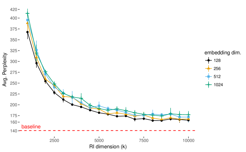
Figure 6: Average test perplexity of best models selected based on validation perplexity for multiple embedding sizes $m\in\{128,256,512,1024\}$ aggregated by number of non-zero entries $s\in\{2,8,16\}$. The number of hidden units was set to $256$.

Increasing the size of the embedding features $m$ seems to yield worse perplexity. We found that models with more parameters where overfitting the training set, thus explaining the worse results. More aggressive regularisation (higher dropout probabilities) seems to alleviate the problem, but for embedding and hidden layer sizes of $1024$ there is either no improvement, or the improvement is marginal.

Table 1: Average test perplexity for the best models selected based on validation perplexity aggregated by number of active units (see figure 6). The number of hidden units was set to $256$.

			PPL		Epoch
$k$	$m$	$\#p$	Avg.	SD	Avg.	SD
$5,000$	$128$	$0.8$	$182$	$0.2$	$12$	$2.0$
	$256$	$1.6$	$190$	$5.9$	$9$	$1.0$
	$512$	$3.2$	$198$	$9.6$	$8$	$0.0$
	$1,024$	$6.3$	$191$	$2.9$	$8$	$0.0$
$7,500$	$128$	$1.1$	$168$	$3.2$	$12$	$0.5$
	$256$	$1.6$	$176$	$7.6$	$8$	$0.0$
	$512$	$3.2$	$176$	$5.2$	$7$	$0.5$
	$1,024$	$8.9$	$178$	$4.6$	$7$	$1.2$
$10,000$	$128$	$1.4$	$164$	$1.4$	$13$	$2.5$
	$256$	$2.8$	$167$	$8.1$	$8$	$0.0$
	$512$	$5.7$	$172$	$12.6$	$8$	$0.6$
	$1,024$	$11$	$177$	$8.4$	$7$	$1.0$
baseline
$10,000$	$128$	$1.4$	$141$	$1.4$	$14$	$1.1$

We then looked at the influence of number of non-zero entries $s$ in the random index vectors for the NRP models, by aggregating the results by embedding size. Figure 7 shows that different values of $s$ do not affect the performance significantly. We should note that this parameter does affect the model performance in terms of perplexity (although marginally) and should be optimised if the goal is to produce the best possible model for a given data set.

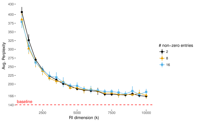
Figure 7: Average test perplexity of the best models selected based on validation perplexity for random indices with a number of non-zero entries $s\in\{2,8,16\}$ aggregated by embedding size $m\in\{128,256,512,1024\}$. The number of hidden units was set to $256$.

The number of epochs to convergence is correlated with the number of trainable parameters (as we will see when comparing these early explorations with later results), but it does not differ significantly between NRP and baseline models (see tables 1 and 2).

Table 2: Average test perplexity of the best models selected based on validation perplexity, aggregated by embedding size $m$ (see figure 7) for multiple values of input vector dimension $k$ and number of non-zero input values $s$. The number of hidden units was set to $256$. Dropout probability is set to $0.05$. $\#p$ is the approximate number of trainable parameters in millions.

			PPL		Epoch
$k$	$s$	$\#p$	Avg.	SD	Avg.	SD
$5,000$	$2$	$0.8$	$186$	$3.4$	$10$	$3.3$
	$8$		$189$	$7.8$	$9$	$1.9$
	$16$		$195$	$10.0$	$9$	$1.5$
$7,500$	$2$	$1.1$	$170$	$3.8$	$9$	$2.5$
	$8$		$175$	$6.2$	$9$	$3.1$
	$16$		$179$	$6.0$	$9$	$2.5$
$10,000$	$2$	$1.4$	$165$	$1.8$	$9$	$3.5$
	$8$		$168$	$9.8$	$8$	$1.2$
	$16$		$177$	$8.7$	$9$	$3.1$
baseline
$10,000$	$1$	$1.4$	$141$	$1.4$	$14$	$1.1$

Finally, in our early explorations, we looked at two different questions. First, we wanted to find out if there was a difference in performance between NRP models using ternary random indices with values $\in\{-1,0,1\}$) and models using binary random indices (with values $\in\{0,1\}$). Second, we wanted to find if redundancy (having more non-zero entries) is key to NRP model performance. To answer this second question, we tested models that used random indices with a single non-zero value. Under this scenario, different words can share the same feature vector. Figure 8 shows the results for this experiment, in which we tested models with these $3$ configurations.

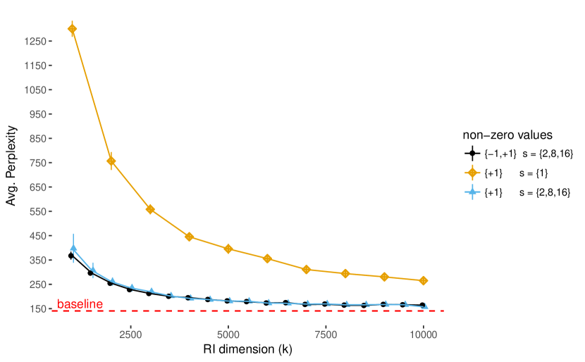
Figure 8: Average test perplexity of best models selected based on validation perplexity for random indices constructed from typical ternary random indices with non-zero entries having values $\in\{+1,1\}$; random indices with a single positive non-zero entry $\{+1\}s\in\{1\}$; and binary random index vectors with non-zero entries $\in\{+1\}$.

We can see that models having a single non-zero positive entry $s=1$ do much worse than any other configuration. Having just two non-zero entries $s>=2$ seems to be enough to improve the model perplexity. A second result we got from this experiment was that using binary and ternary random indices yields similar results, with binary indices displaying an increased variance for lower values of random index dimension $k$. We think this increase in variance is due to the fact that lower-dimensional binary random indices have a higher probability of collisions and thus disambiguation of such collisions becomes harder for our neural network models. As for why the results are similar, we should note that the near-orthogonality properties of random indices are still maintained whether or not we use ternary representations. Moreover, the feature layer (or embeddings) is itself symmetric, having equally distributed positive and negative weights, so the symmetry in the input space should not have much impact on the model performance.

4.3 The role of regularisation

In the next set of experiments, we look at the role of dropout probability in both the baseline and NRP models. Figure 9 shows the test perplexity scores for the baseline model using different embedding sizes $m$ and dropout probability values $p=\{0.05,0.25,0.3\}$. The number of hidden units is fixed at $h=256$.

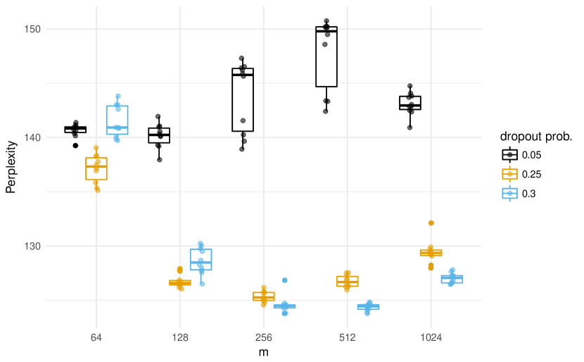
Figure 9: Baseline model test perplexity of best models selected based on validation perplexity for multiple values of embedding size $m$ and dropout probability.

We can see that keeping the dropout probability at the previously used value $0.05$ makes the model perform worse for embedding size values $m>128$. We found out that larger models were heavily overfitting the training set, which explains why more aggressive dropout rates give us better results for larger feature spaces. After extensive testing of this hypothesis and parameter tuning, we recommend the use of higher dropout when increasing the size of the hidden layer (figure 10, and table 3).

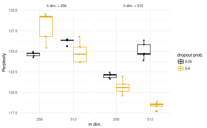
Figure 10: Baseline model test perplexity of best models selected based on validation perplexity for multiple values of embedding size $m$, hidden layer number of units $h$ and dropout probability.

Looking at the results for NRP models (figure 11, table 4), we can see that the best results are achieved with larger models and higher dropout probability. We should mention that even with half the embedding parameters (using random indices of dimension $k=5k$ to encode a vocabulary of $10k$ words), we get reasonably good models with test perplexities of $145$ to $150$ using only, $1.6$ to $1.9$ million parameters (table 4). We can compare this with the perplexity scores obtain in (Pham et al., 2016) when using the same dataset and partitions. The model from (Bengio et al., 2003) with approximately $4.5$ million parameters gets a test perplexity of $147$ to $152$. This is of course not a fair comparison, because we would need to optimise both models using the best possible hyper-parameter values and regularisation methods, but it does confirm our main hypothesis: that we can we can learn language models using a random projection of the input space.

Table 3: Average test perplexity and convergence epoch for different configurations of the baseline model with multiple values of embedding size $m$, number of hidden units $h$ and weight dropout probability drop. $\#p$ is the approximate number of trainable parameters in millions.

				PPL		Epoch
$m$	$h$	$\#p$	drop	Avg.	SD	Avg.	SD
$256$	$256$	$2.8$	$.25$	$125$	$0.3$	$22$	$1.5$
			$.40$	$128$	$1.8$	$22$	$2.5$
	$512$	$3.2$	$.25$	$122$	$0.3$	$19$	$2.0$
			$.40$	$121$	$0.9$	$23$	$1.6$
$512$	$256$	$5.8$	$.25$	$126$	$0.3$	$20$	$1.6$
			$.40$	$125$	$1.3$	$22$	$1.9$
	$512$	$6.4$	$.25$	$125$	$1.0$	$16$	$1.8$
			$.40$	$\mathbf{118}$	$0.4$	$22$	$1.3$

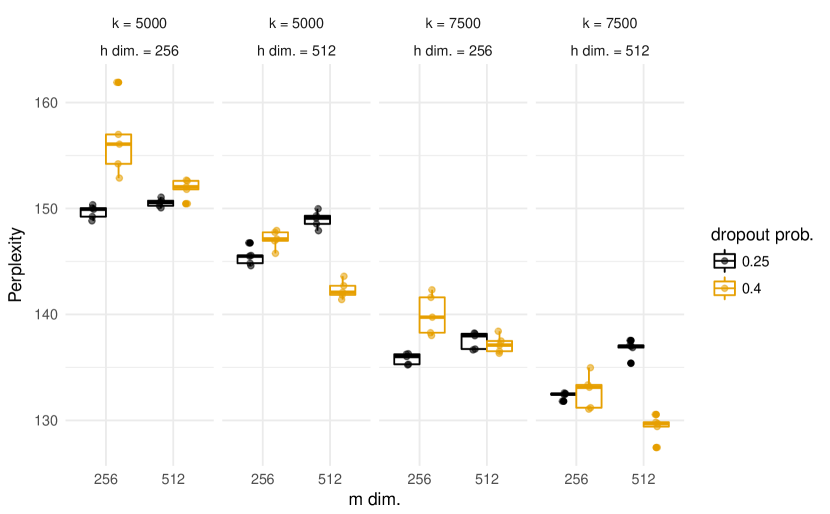
Figure 11: NRP model test perplexity of best models selected based on validation perplexity for multiple values of random index size $k$, embedding size $m$, hidden layer number of units $h$ and dropout probability.

Table 4: Average test perplexity and convergence epoch for different configurations of NRP models with multiple values of random index dimension $k$ embedding size $m$, number of hidden units $h$ and weight dropout probability drop. The number of non-zero entries in the RI is set fo $4$. $\#p$ is the approximate number of trainable parameters in millions.

					PPL		Epoch
$k$	$m$	$h$	$\#p$	drop	Avg.	SD	Avg.	SD
$5,000$	$256$	$256$	$1.6$	$.25$	$149$	$0.6$	$23$	$1.2$
				$.40$	$156$	$3.5$	$25$	$3.4$
		$512$	$1.9$	$.25$	$145$	$0.8$	$22$	$1.7$
				$.40$	$147$	$0.9$	$25$	$1.1$
	$512$	$256$	$3.2$	$.25$	$150$	$0.4$	$21$	$1.5$
				$.40$	$151$	$0.9$	$24$	$0.9$
		$512$	$3.8$	$.25$	$149$	$0.8$	$19$	$2.3$
				$.40$	$\mathbf{142}$	$0.9$	$24$	$1.0$
$7,500$	$256$	$256$	$2.2$	$.25$	$136$	$0.5$	$22$	$1.3$
				$.40$	$140$	$1.9$	$26$	$2.9$
		$512$	$2.5$	$.25$	$132$	$0.3$	$21$	$0.8$
				$.40$	$133$	$1.6$	$24$	$2.3$
	$512$	$256$	$4.4$	$.25$	$137$	$0.8$	$21$	$0.8$
				$.40$	$137$	$0.8$	$24$	$1.7$
		$512$	$5.1$	$.25$	$137$	$0.8$	$18$	$1.8$
				$.40$	$\mathbf{129}$	$1.2$	$23$	$1.5$

Additional tests showed us that we cannot go much further with dropout probabilities, so we stuck to a maximum value of $0.4$, since it yielded the best results for both the baseline and models using random projections. One weakness in our methodology was that hyper-parameter exploration was done based on grid search and intuition about model behaviour – mostly because each model run is very expensive. While our goal is not to find the best possible baseline and NRP models, but to show that we can achieve qualitatively similar results with random projections and a reduced embedding space, in future work this methodological aspect will be improved by replacing grid search by a more appropriate method such as Bayesian Optimisation (Snoek et al., 2012). This way, we can compare the best possible models, since many hyper-parameters should be tuned to particular model architectures.

4.4 Best model approximation

Finally, we analyse the performance of an NRP model with the best configuration we found in previous experiments, and compare it with the best baseline model found. We performed multiple runs with different values of random index dimension $k$. The results can be seen in figure 12.

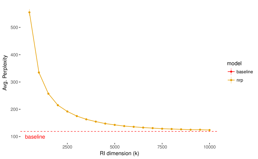
Figure 12: Average test perplexity for the best NRP and baseline configurations found (see tables 3, and 4) with $m=h=512$ and dropout probability $0.6$ for multiple NRP random index vector dimension values $k$.

As with our early experiments, the perplexity decays exponentially with the increase of the random index dimension $k$. One key difference is that this decay is much more accentuated and model test perplexity converges to values closer to the baseline, with lower-dimensional random indices. In summary, random projections seem to be a viable technique to build models with comparable predictive power, with a much lower number of parameters and without the necessity of a priori knowledge of the dimension of the lexicon to be used. Proper regularisation and model size tuning was key to achieve good results. NRP models are also more sensitive to hyper-parameter values and model size than the baseline model. This was an expected result, since the problem of estimating distributed representations using a compressed input space is harder than using dedicated feature vectors for each unique input.

5 Conclusion and future work

In this work ,we investigated the potential of using random projections as an encoder for neural network models for language modelling. The results extend beyond this sequence prediction task and can applicable to any neural-network-based modelling problem that involves the modelling of discrete input patterns.

We showed that using random projections allows us to obtain perplexity scores comparable to a model that uses an $1\text{-of-}V$ encoding, while reducing the number of necessary trainable parameters. On top of this, our approach opens multiple interesting research directions.

Random projections introduce additional computational complexity in the output layer ,because to obtain the output probabilities we need the vector representations for all the existing words –and these representations are a combination of multiple features. The problem only arises because we need to output a probability distribution over words,. However,our approach is compatible with approximation techniques such as Noise Constrastive Estimation (NCE)(Mnih & Teh, 2012)., with benefits that we will demonstrate in a short while. Another future research direction is to answer the question of whether or not more powerful neural network architectures (such RNNs or LSTMs) can yield better results using random projections –possibly using even smaller random index dimensions and embedding spaces.

We have introduced a new simple baseline on the small, but widely used Penn Treebank dataset. Our baseline model combined the energy-based principles from the work in (Mnih & Hinton, 2007) with the simple feedforward seminal neural network architecture proposed in (Bengio et al., 2003), and with a recent regularisation technique (dropout (Srivastava et al., 2014)). Model performance and training speed were also improved by using rectifier linear units (ReLUs) in the hidden layers, similarly to the baseline proposed in (Pham et al., 2016). The result was a very simple architecture with a low number of parameters, and a performance comparable to similar models in the literature. We tested our random projection encoder in an energy-based neural network architecture, because this would allow us to extend this work beyond the prediction of vocabulary distributions. The fact that we can predict distributed representations,means that we can encode –and make predictions about– more complex patterns. In future work, we intend to explore whether or not we can use random projections to exploit sequence information, linguistic knowledge, or structured input patterns similarly to the approaches in (Plate, 1995; Cohen et al., 2009; Basile et al., 2011).

References

- Achlioptas (2003) Achlioptas, Dimitris. Database-friendly random projections: Johnson-lindenstrauss with binary coins. Journal of computer and System Sciences, 66(4):671–687, 2003.
- Arisoy et al. (2012) Arisoy, Ebru, Sainath, Tara N., Kingsbury, Brian, and Ramabhadran, Bhuvana. Deep neural network language models. In Proceedings of the NAACL-HLT 2012 Workshop: Will We Ever Really Replace the N-gram Model? On the Future of Language Modeling for HLT, pp. 20–28. Association for Computational Linguistics, 2012.
- Basile et al. (2011) Basile, Pierpaolo, Caputo, Annalina, and Semeraro, Giovanni. Encoding syntactic dependencies by vector permutation. In Proceedings of the GEMS 2011 Workshop on Geometrical Models of Natural Language Semantics, pp. 43–51. Association for Computational Linguistics, 2011.
- Bengio et al. (2003) Bengio, Yoshua, Ducharme, Réjean, Vincent, Pascal, and Janvin, Christian. A neural probabilistic language model. The Journal of Machine Learning Research, 3:1137–1155, 2003.
- Brown et al. (1992) Brown, Peter F., Desouza, Peter V., Mercer, Robert L., Pietra, Vincent J. Della, and Lai, Jenifer C. Class-based n-gram models of natural language. Computational linguistics, 18(4):467–479, 1992.
- Clevert et al. (2015) Clevert, Djork-Arné, Unterthiner, Thomas, and Hochreiter, Sepp. Fast and Accurate Deep Network Learning by Exponential Linear Units (ELUs). arXiv:1511.07289 [cs], November 2015.
- Cohen et al. (2009) Cohen, Trevor, Schvaneveldt, Roger W, and Rindflesch, Thomas C. Predication-based semantic indexing: Permutations as a means to encode predications in semantic space. In AMIA Annual Symposium Proceedings, volume 2009, pp. 114. American Medical Informatics Association, 2009.
- Dauphin et al. (2016) Dauphin, Yann N., Fan, Angela, Auli, Michael, and Grangier, David. Language modeling with gated convolutional networks. arXiv:1612.08083 [cs], 2016.
- Elman (1990) Elman, Jeffrey L. Finding structure in time. Cognitive science, 14(2):179–211, 1990.
- Feyerabend (1955) Feyerabend, Paul. Wittgenstein’s Philosophical Investigations. The Philosophical Review, 64(3):449, July 1955.
- Gribonval et al. (2015) Gribonval, Rémi, Jenatton, Rodolphe, and Bach, Francis. Sparse and spurious: Dictionary learning with noise and outliers. IEEE Transactions on Information Theory, 61(11):6298–6319, 2015.
- Gutmann & Hyvärinen (2012) Gutmann, Michael U. and Hyvärinen, Aapo. Noise-contrastive estimation of unnormalized statistical models, with applications to natural image statistics. Journal of Machine Learning Research, 13:307–361, 2012.
- Halko et al. (2011) Halko, Nathan, Martinsson, Per-Gunnar, and Tropp, Joel A. Finding structure with randomness: Probabilistic algorithms for constructing approximate matrix decompositions. SIAM review, 53(2):217–288, 2011.
- He et al. (2015) He, Kaiming, Zhang, Xiangyu, Ren, Shaoqing, and Sun, Jian. Delving deep into rectifiers: Surpassing human-level performance on imagenet classification. In Proceedings of the 2015 IEEE ICCV, pp. 1026–1034. IEEE Computer Society, 2015. doi: 10.1109/ICCV.2015.123.
- Hegde et al. (2016) Hegde, Chinmay, Indyk, Piotr, and Schmidt, Ludwig. Fast recovery from a union of subspaces. In Advances in Neural Information Processing Systems, pp. 4394–4402, 2016.
- Hinton (1986) Hinton, Geoffrey E. Learning distributed representations of concepts. In Proceedings of the eighth annual conference of the cognitive science society, volume 1, pp. 12. Amherst, MA, 1986.
- Indyk (2001) Indyk, P. Algorithmic aspects of low-distortion geometric embeddings. In Annual symposium on foundations of computer science (FOCS), 2001.
- Johnson & Lindenstrauss (1984) Johnson, William B and Lindenstrauss, Joram. Extensions of lipschitz mappings into a hilbert space. Contemporary mathematics, 26(189):1, 1984.
- Jozefowicz et al. (2016) Jozefowicz, Rafal, Vinyals, Oriol, Schuster, Mike, Shazeer, Noam, and Wu, Yonghui. Exploring the Limits of Language Modeling. arXiv preprint arXiv:1602.02410, 2016.
- Kanerva (1988) Kanerva, Pentti. Sparse distributed memory. MIT press, 1988.
- Kanerva (2009) Kanerva, Pentti. Hyperdimensional computing: An introduction to computing in distributed representation with high-dimensional random vectors. Cognitive Computation, 1(2):139–159, 2009.
- Kanerva et al. (2000) Kanerva, Pentti, Kristofersson, Jan, and Holst, Anders. Random indexing of text samples for latent semantic analysis. In Proceedings of the 22nd annual conference of the cognitive science society, 2000.
- Kaski (1998) Kaski, Samuel. Dimensionality reduction by random mapping: fast similarity computation for clustering. In Neural Networks Proceedings, volume 1, pp. 413–418, May 1998.
- Kim et al. (2016) Kim, Yoon, Jernite, Yacine, Sontag, David, and Rush, Alexander M. Character-aware neural language models. In AAAI, 2016.
- Kingma & Ba (2014) Kingma, Diederik P. and Ba, Jimmy. Adam: A method for stochastic optimization. In Proceedings of the 3rd ICLR, 2014. URL http://arxiv.org/abs/1412.6980.
- Kneser & Ney (1995) Kneser, Reinhard and Ney, Hermann. Improved backing-off for m-gram language modeling. In Acoustics, Speech, and Signal Processing, 1995. ICASSP-95., 1995 International Conference on, volume 1, pp. 181–184. IEEE, 1995.
- Koehn (2010) Koehn, Philipp. Statistical machine translation. Cambridge University Press, 2010. ISBN 0521874157, 9780521874151.
- Landauer & Dumais (1997) Landauer, Thomas K. and Dumais, Susan T. A solution to Plato’s problem: The latent semantic analysis theory of acquisition, induction, and representation of knowledge. Psychological review, 104(2):211, 1997.
- Lecun et al. (2006) Lecun, Yann, Chopra, Sumit, Hadsell, Raia, Ranzato, Marc Aurelio, and Huang, Fu Jie. A tutorial on energy-based learning. In Predicting structured data. MIT Press, 2006.
- Levy et al. (2014) Levy, Omer, Goldberg, Yoav, and Ramat-Gan, Israel. Linguistic Regularities in Sparse and Explicit Word Representations. In CoNLL, pp. 171–180, 2014.
- Ling & Dyer (2015) Ling, Yulia Tsvetkov Manaal Faruqui Wang and Dyer, Guillaume Lample Chris. Evaluation of word vector representations by subspace alignment. In Proceedings of the 2015 Conference on Empirical Methods in Natural Language Processing, pp. 2049–2054, 2015.
- Marcus et al. (1993) Marcus, Mitchell P., Marcinkiewicz, Mary Ann, and Santorini, Beatrice. Building a large annotated corpus of English: The Penn Treebank. Computational linguistics, 19(2):313–330, 1993.
- Mikolov et al. (2013a) Mikolov, Tomas, Sutskever, Ilya, Chen, Kai, Corrado, Greg, and Dean, Jeffrey. Distributed representations of words and phrases and their compositionality. In Proceedings of the 26th International Conference on Neural Information Processing Systems - Volume 2, NIPS’13, pp. 3111–3119, USA, 2013a. Curran Associates Inc.
- Mikolov et al. (2011) Mikolov, Tomáš, Deoras, Anoop, Kombrink, Stefan, Burget, Lukáš, and Černockỳ, Jan. Empirical evaluation and combination of advanced language modeling techniques. In Twelfth Annual Conference of the International Speech Communication Association, 2011.
- Mikolov et al. (2013b) Mikolov, Tomáš, Chen, Kai, Corrado, Greg, and Dean, Jeffrey. Efficient estimation of word representations in vector space. arXiv preprint arXiv:1301.3781, 2013b.
- Mikolov et al. (2012) Mikolov, Tomáš, Sutskever, Ilya, Deoras, Anoop, Le, Hai-Son, Kombrink, Stefan, and Cernocky, Jan. Subword language modeling with neural networks. preprint (http://www. fit. vutbr. cz/imikolov/rnnlm/char. pdf), 2012.
- Mnih & Hinton (2007) Mnih, Andriy and Hinton, Geoffrey. Three new graphical models for statistical language modelling. In Proceedings of the 24th international conference on Machine learning, pp. 641–648. ACM, 2007.
- Mnih & Teh (2012) Mnih, Andriy and Teh, Yee Whye. A fast and simple algorithm for training neural probabilistic language models. arXiv preprint arXiv:1206.6426, 2012. URL http://arxiv.org/abs/1206.6426.
- Mnih et al. (2009) Mnih, Andriy, Yuecheng, Zhang, and Hinton, Geoffrey. Improving a statistical language model through non-linear prediction. Neurocomputing, 72(7-9):1414–1418, March 2009. ISSN 09252312.
- Morin & Bengio (2005) Morin, Frederic and Bengio, Yoshua. Hierarchical probabilistic neural network language model. In Proceedings of the international workshop on artificial intelligence and statistics, pp. 246–252, 2005.
- Papadimitriou et al. (1998) Papadimitriou, Christos H., Tamaki, Hisao, Raghavan, Prabhakar, and Vempala, Santosh. Latent semantic indexing: A probabilistic analysis. In Proceedings of the Seventeenth ACM SIGACT-SIGMOD-SIGART Symposium on Principles of Database Systems, PODS ’98, pp. 159–168. ACM, 1998.
- Pham et al. (2016) Pham, Ngoc-Quan, Kruszewski, German, and Boleda, Gemma. Convolutional Neural Network Language Models. In EMNLP, pp. 1153–1162, 2016.
- Pinker (2010) Pinker, Steven. The cognitive niche: Coevolution of intelligence, sociality, and language. In Proceedings of the National Academy of Sciences, volume 107, pp. 8993–8999, 2010.
- Plate (1995) Plate, Tony A. Holographic reduced representations. IEEE Transactions on Neural networks, 6(3):623–641, 1995.
- Ponte & Croft (1998) Ponte, Jay M and Croft, W Bruce. A language modeling approach to information retrieval. In Proceedings of the 21st annual international ACM SIGIR conference on Research and development in information retrieval, pp. 275–281. ACM, 1998.
- Ritter & Kohonen (1989) Ritter, Helge and Kohonen, Teuvo. Self-organizing semantic maps. Biological cybernetics, 61(4):241–254, 1989.
- Serban et al. (2016) Serban, Iulian V., Sordoni, Alessandro, Bengio, Yoshua, Courville, Aaron, and Pineau, Joelle. Building end-to-end dialogue systems using generative hierarchical neural network models. arXiv:1507.04808 [cs], pp. 3776–3784, 2016.
- Snoek et al. (2012) Snoek, Jasper, Larochelle, Hugo, and Adams, Ryan P. Practcal bayesian optimization of machine learning algorithms. In Advances in neural information processing systems, pp. 2951–2959, 2012.
- Socher et al. (2011) Socher, Richard, Lin, Cliff C, Manning, Chris, and Ng, Andrew Y. Parsing natural scenes and natural language with recursive neural networks. In Proceedings of the 28th international conference on machine learning (ICML-11), pp. 129–136, 2011.
- Srivastava et al. (2014) Srivastava, Nitish, Hinton, Geoffrey, Krizhevsky, Alex, Sutskever, Ilya, and Salakhutdinov, Ruslan. Dropout: A simple way to prevent neural networks from overfitting. Journal of Machine Learning Research, 15:1929–1958, 2014.
- Vaswani et al. (2017) Vaswani, Ashish, Shazeer, Noam, Parmar, Niki, Uszkoreit, Jakob, Jones, Llion, Gomez, Aidan N., Kaiser, Lukasz, and Polosukhin, Illia. Attention Is All You Need. arXiv:1706.03762 [cs], June 2017.
- Zhang & LeCun (2015) Zhang, Xiang and LeCun, Yann. Text understanding from scratch. arXiv preprint arXiv:1502.01710, 2015. URL http://arxiv.org/abs/1502.01710.