Quantum-assisted quantum compiling
Abstract
Compiling quantum algorithms for near-term quantum computers (accounting for connectivity and native gate alphabets) is a major challenge that has received significant attention both by industry and academia. Avoiding the exponential overhead of classical simulation of quantum dynamics will allow compilation of larger algorithms, and a strategy for this is to evaluate an algorithm’s cost on a quantum computer. To this end, we propose a variational hybrid quantum-classical algorithm called quantum-assisted quantum compiling (QAQC). In QAQC, we use the overlap between a target unitary and a trainable unitary as the cost function to be evaluated on the quantum computer. More precisely, to ensure that QAQC scales well with problem size, our cost involves not only the global overlap but also the local overlaps with respect to individual qubits. We introduce novel short-depth quantum circuits to quantify the terms in our cost function, and we prove that our cost cannot be efficiently approximated with a classical algorithm under reasonable complexity assumptions. We present both gradient-free and gradient-based approaches to minimizing this cost. As a demonstration of QAQC, we compile various one-qubit gates on IBM’s and Rigetti’s quantum computers into their respective native gate alphabets. Furthermore, we successfully simulate QAQC up to a problem size of 9 qubits, and these simulations highlight both the scalability of our cost function as well as the noise resilience of QAQC. Future applications of QAQC include algorithm depth compression, black-box compiling, noise mitigation, and benchmarking.
1 Introduction
Factoring [1], approximate optimization [2], and simulation of quantum systems [3] are some of the applications for which quantum computers have been predicted to provide speedups over classical computers. Consequently, the prospect of large-scale quantum computers has generated interest from various sectors, such as the financial and pharmaceutical industries. Currently available quantum computers are not large-scale but rather have been called noisy intermediate-scale quantum (NISQ) computers [4]. A proof-of-principle demonstration of quantum supremacy with a NISQ device may be coming soon [5, 6]. Nevertheless, demonstrating the practical utility of NISQ computers appears to be a more difficult task.
While improvements to NISQ hardware are continuously being made by experimentalists, quantum computing theorists can contribute to the utility of NISQ devices by developing software. This software would aim to adapt textbook quantum algorithms (e.g., for factoring or quantum simulation) to NISQ constraints. NISQ constraints include: (1) limited numbers of qubits, (2) limited connectivity between qubits, (3) restricted (hardware-specific) gate alphabets, and (4) limited circuit depth due to noise. Algorithms adapted to these constraints will likely look dramatically different from their textbook counterparts.
These constraints have increased the importance of the field of quantum compiling. In classical computing, a compiler is a program that converts instructions into assembly language so that they can be read and executed by a computer. Similarly, a quantum compiler would take a high-level algorithm and convert it into a lower-level form that could be executed on a NISQ device. Already, a large body of literature exists on classical approaches for quantum compiling, e.g., using temporal planning [7, 8], machine learning [9], and other techniques [10, 11, 12, 13, 14, 15, 16, 17].
A recent exciting idea is to use quantum computers themselves to train parametrized quantum circuits, as proposed in Refs. [2, 18, 19, 20, 21, 22, 23, 24, 25]. The cost function to be minimized essentially defines the application. For example, in the variational quantum eigensolver (VQE) [18] and the quantum approximate optimization algorithm (QAOA) [2], the application is ground state preparation, and hence the cost is the expectation value of the associated Hamiltonian. Another example is training error-correcting codes [19], where the cost is the average code fidelity. In light of these works, it is natural to ask: what is the relevant cost function for the application of quantum compiling?
In this work, we introduce quantum-assisted quantum compiling (QAQC, pronounced “Quack”). The goal of QAQC is to compile a (possibly unknown) target unitary to a trainable quantum gate sequence. A key feature of QAQC is the fact that the cost is computed directly on the quantum computer. This leads to an exponential speedup (in the number of qubits involved in the gate sequence) over classical methods to compute the cost, since classical simulation of quantum dynamics is exponentially slower than quantum simulation. Consequently, one should be able to optimally compile larger-scale gate sequences using QAQC, whereas classical approaches to optimal quantum compiling will be limited to smaller gate sequences.111We note that classical compilers may be applied to large-scale quantum algorithms, but they are limited to local compiling. We thus emphasize the distinction between translating the algorithm to the native alphabet with simple, local compiling and optimal compiling. Local compiling may reach partial optimization but in order to discover the shortest circuit one may need to use a holistic approach, where the entire algorithm is considered, which requires a quantum computer for compiling.
We carefully define a cost function for QAQC that satisfies the following criteria:
-
1.
It is faithful (vanishing if and only if the compilation is exact);
-
2.
It is efficient to compute on a quantum computer;
-
3.
It has an operational meaning;
-
4.
It scales well with the size of the problem.
A potential candidate for a cost function satisfying these criteria is the Hilbert-Schmidt inner product between a target unitary and a trainable unitary :
| (1) |
It turns out, however, that this cost function does not satisfy the last criterion. We thus use Eq. (1) only for small-scale problems. For general, large-scale problems, we define a cost function satisfying all criteria. This cost involves a weighted average of the global overlap in (1) with localized overlaps, which quantify the overlap between and with respect to individual qubits.
We prove that computing our cost function is -hard, where is the class of problems that can be efficiently solved in the one-clean-qubit model of computation [26]. Since is classically hard to simulate [27], this implies that no classical algorithm can efficiently compute our cost function. We remark that an alternative cost function might be a worst-case distance measure (such as diamond distance), but such measures are known to be -complete [28] and hence would violate criterion 2 in our list above. In this sense, our cost function appears to be ideal.
Furthermore, we present novel short-depth quantum circuits for efficiently computing the terms in our cost function. Our circuits achieve short depth by avoiding implementing controlled versions of and , and by implementing and in parallel. We also present, in Appendix F, circuits that compute the gradient of our cost function. One such circuit is a generalization of the well-known Power of One Qubit [26] that we call the Power of Two Qubits.
As a proof-of-principle, we implement QAQC on both IBM’s and Rigetti’s quantum computers, and we compile various one-qubit gates to the native gate alphabets used by these hardwares. To our knowledge, this is the first compilation of a target unitary with cost evaluation on actual NISQ hardware. In addition, we successfully implement QAQC on both a noiseless and noisy simulator for problems as large as 9-qubit unitaries. These larger scale implementations illustrate the scalability of our cost function, and in the case of the noisy simulator, show a somewhat surprising resilience to noise.

 denotes the -rotation gate , while
  represents the -pulse given by the -rotation gate . Both gates are natively implemented on commercial hardware [29, 30]. (a) Compressing the depth of a given gate sequence to a shorter-depth gate sequence in terms of native hardware gates. (b) Uploading a black-box unitary. The black box could be an analog unitary , for an unknown Hamiltonian , that one wishes to convert into a gate sequence to be run on a gate-based quantum computer. (c) Training algorithms in the presence of noise to learn noise-resilient algorithms (e.g., via gates that counteract the noise). Here, the unitary is performed on high-quality, pristine qubits and is performed on noisy ones. (d) Benchmarking a quantum computer by compiling a unitary on noisy qubits and learning the gate sequence on high-quality qubits.
In what follows, we first discuss several applications of interest for QAQC. Section 3 provides a general outline of the QAQC algorithm. Section 4 presents our short-depth circuits for cost evaluation on a quantum computer. Section 5 states that our cost function is classically hard to simulate. Sections 6 and 7, respectively, present small-scale and larger-scale implementations of QAQC.
2 Applications of QAQC
Figure 1 illustrates four potential applications of QAQC. Suppose that there exists a quantum algorithm to perform some task, but its associated gate sequence is longer than desired. As shown in Fig. 1(a), it is possible to use QAQC to shorten the gate sequence by accounting for the NISQ constraints of the specific computer. This depth compression goes beyond the capabilities of classical compilers.
As a simple example, consider the quantum Fourier transform on qubits. Its textbook algorithm is written in terms of Hadamard gates and controlled-rotation gates [31], which may need to be compiled into the native gate alphabet. The number of gates in the textbook algorithm is , so one could use a classical compiler to locally compile each gate. But this could lead to a sub-optimal depth since the compilation starts from the textbook structure. In contrast, QAQC is unbiased with respect to the structure of the gate sequence, taking a holistic approach to compiling as opposed to a local one. Hence, in principle, it can learn the optimal gate sequence for given hardware. Note that classical compilers cannot take this holistic approach for large due to the exponential scaling of the matrix representations of the gates.
Alternatively, consider the problem of simulating the dynamics of a given quantum system with an unknown Hamiltonian (via ) on a quantum computer. We call this problem black-box uploading because by simulating the black-box, i.e., the unitary , we are “uploading” the unitary onto the quantum computer. This scenario is depicted in Fig. 1(b). QAQC could be used to convert an analog black-box unitary into a gate sequence on a digital quantum computer.
Finally, we highlight two additional applications that are the opposites of each other. These two applications can be exploited when the quantum computer has some pristine qubits (qubits with low noise) and some noisy qubits. We emphasize that, in this context, “noisy qubits” refers to coherent noise such as systematic gate biases, where the gate rotation angles are biased in a particular direction. In contrast, we consider incoherent noise (e.g., and noise) later in this article, see Section 7.2.
Consider Fig. 1(c). Here, the goal is to implement a CNOT gate on two noisy qubits. Due to the noise, to actually implement a true CNOT, one has to physically implement a dressed CNOT, i.e., a CNOT surrounded by one-qubit unitaries. QAQC can be used to learn the parameters in these one-qubit unitaries. By choosing the target unitary to be a CNOT on a pristine (i.e., noiseless) pair of qubits, it is possible to learn the unitary that needs to be applied to the noisy qubits in order to effectively implement a CNOT. We call this application noise-tailored algorithms, since the learned algorithms are robust to the noise process on the noisy qubits.
Figure 1(d) depicts the opposite process, which is benchmarking. Here, the unitary acts on a noisy set of qubits, and the goal is to determine what the equivalent unitary would be if it were implemented on a pristine set of qubits. This essentially corresponds to learning the noise model, i.e., benchmarking the noisy qubits.
3 The QAQC Algorithm
3.1 Approximate compiling
The goal of QAQC is to take a (possibly unknown) unitary and return a gate sequence , executable on a quantum computer, that has approximately the same action as on any given input state (up to possibly a global phase factor). The notion of approximate compiling [32, 33, 34, 35, 36, 37] requires an operational figure-of-merit that quantifies how close the compilation is to exact. A natural candidate is the probability for the evolution under to mimic the evolution under . Hence, consider the overlap between and , averaged over all input states . This is the fidelity averaged over the Haar distribution,
| (2) |
We call an exact compilation of if . If , where , then we call an -approximate compilation of , or simply an approximate compilation of .
As we will see, the quantity has a connection to our cost function, defined below, and hence our cost function has operational relevance to approximate compiling. Minimizing our cost function is related to maximizing , and thus is related to compiling to a better approximation.
QAQC achieves approximate compiling by training a gate sequence of a fixed length , which may even be shorter than the length required to exactly compile . As one increases , one can further minimize our cost function. The length can therefore be regarded as a parameter that can be tuned to obtain arbitrarily good approximate compilations of .

3.2 Discrete and continuous parameters
The gate sequence should be expressed in terms of the native gates of the quantum computer being used. Consider an alphabet of gates that are native to the quantum computer of interest. Here, is a continuous parameter, and is a discrete parameter that identifies the type of gate and which qubits it acts on. For a given quantum computer, the problem of compiling to a gate sequence of length is to determine
| (3) |
where
| (4) |
is the trainable unitary. Here, is a function of the sequence of parameters describing which gates from the native gate set are used and of the continuous parameters associated with each gate. The function is the cost, which quantifies how close the trained unitary is to the target unitary. We define the cost below to have the properties: for all unitaries and , and if and only if (possibly up to a global phase factor).
The optimization in (3) contains two parts: discrete optimization over the finite set of gate structures parameterized by , and continuous optimization over the parameters characterizing the gates within the structure. Our quantum-classical hybrid strategy to perform the optimization in (3) is illustrated in Fig. 2. In the next subsection, we present a general, ansatz-free approach to optimizing our cost function, which may be useful for systems with a small number of qubits. In the subsection following that, we present an ansatz-based approach that would allow the extension to larger system sizes. In each case, we perform the continuous parameter optimization using gradient-free methods as described in Appendix E. We also discuss a method for gradient-based continuous parameter optimization in Appendix F.
3.3 Small problem sizes
Suppose and act on a -dimensional space of qubits, so that . To perform the continuous parameter optimization in (3), we define the cost function
| (5) | ||||
where HST stands for “Hilbert-Schmidt Test” and refers to the circuit used to evaluate the cost, which we introduce in Sec. 4.1. Note that the quantity is simply the fidelity between the pure states obtained by applying and to one half of a maximally entangled state. Consequently, it has an operational meaning in terms of . Indeed, it can be shown [38, 39] that
| (6) |
Also note that for any two unitaries and , if and only if and differ by a global phase factor, i.e., for some . By minimizing , we thus learn an equivalent unitary up to a global phase.
Now, to perform the optimization over gate structures in (3), one strategy is to search over all possible gate structures for a gate sequence length , which can be allowed to vary during the optimization. As the set of gate structures grows exponentially with the number of gates , such a brute force search over all gate structures in order to obtain the best one is intractable in general. To efficiently search through this exponentially large space, we adopt an approach based on simulated annealing. (An alternative approach is genetic optimization, which has been implemented previously to classically optimize quantum gate sequences [40].)
Our simulated annealing approach starts with a random gate structure, then performs continuous optimization over the parameters that characterize the gates in order to minimize the cost function. We then perform a structure update that involves randomly replacing a subset of gates in the sequence with new gates (which can be done in a way such that the sequence length can increase or decrease) and re-optimizing the cost function over the continuous parameters . If this structure change produces a lower cost, then we accept the change. If the cost increases, then we accept the change with probability decreasing exponentially in the magnitude of the cost difference. We iterate this procedure until the cost converges or until a maximum number of iterations is reached.
With a fixed gate sequence length , the approach outlined above will in general lead to an approximate compilation of , which in many cases is sufficient. One strategy for obtaining better and better approximate compilations of is a layered approach illustrated in Fig. 2(a). In this approach, we consider a particular gate sequence length and perform the full structure optimization, as outlined above, to obtain an (approximate) length- compilation of . The optimal gate sequence structure thus obtained can then be concatenated with a new sequence of a possibly different (but fixed) length, whose structure can vary. By performing the continuous parameter optimization over the entire longer gate sequence, and performing the structure optimization over the new additional segment of the gate sequence, we can obtain a better approximate compilation of . Iterating this procedure can then lead to increasingly better approximate compilations of .
3.4 Large problem sizes
We emphasize two potential issues with scaling the above approach to large problem sizes.
First, one may want a guarantee that there exists an exact compilation of within a polynomial size search space for . When performing full structure optimization, as above, the search space size grows exponentially in the length of the gate sequence. This implies that the search space size grows exponentially in , if one chooses to grow polynomially in . Indeed, one would typically require to grow polynomially in if one is interested in exact compilation, since the number of gates in itself grows polynomially in for many applications. (Note that this issue arises if one insists on exact, instead of approximate, compiling.)
Second, and arguably more importantly, the cost is exponentially fragile. The inner product between and will be exponentially suppressed for random choices of , which means that will be very close to one for most unitaries . Hence, for random unitaries , the number of calls to the quantum computer needed to resolve differences in the cost to a given precision will grow exponentially.
The first issue can be addressed with an efficiently parameterized ansatz for . With an ansatz, only the continuous parameters need to be optimized in . The parameters are fixed, which means that structure updates are not required. This fixed structure approach is depicted in Fig. 2(b). One can choose an ansatz such that the number of parameters needed to represent the target unitary is only a polynomial function of . Hence, one should allow the ansatz to be application specific, i.e., to be a function of . As an example, if for a local Hamiltonian , one could choose the ansatz to involve a polynomial number of local interactions. Due to the application-specific nature of the ansatz, the problem is a complex one, hence we leave the issue of finding efficient ansatzes for future work.
Nevertheless, we show a concrete example of a potential ansatz for in Fig. 3. The ansatz is defined by a number of layers, with each layer being a gate sequence of depth two consisting of two-qubit gates acting on neighboring qubits. Consider the following argument. In QAQC, the unitary to be compiled is executed on the quantum computer, so it must be efficiently implementable, i.e., the gate count is polynomial in . Next, note that the gate sequence used to implement can be compiled into in the ansatz in Fig. 3 with only polynomial overhead. This implies that the ansatz in Fig. 3 could exactly describe in only a polynomial number of layers and would hence eliminate the need to search through an exponentially large space. We remark that the ansatz in Fig. 3 may be particularly useful for applications involving compiling quantum simulations of physically relevant systems, as the structure resembles that of the Suzuki-Trotter decomposition [41] for nearest-neighbor Hamiltonians.

Let us now consider the second issue mentioned above: the exponentially suppressed inner product between and for large . To address this, we propose an alternative cost function involving a weighted average between the function in (5) and a “local” cost function:
| (7) |
where and
| (8) |
Here, LHST stands for “Local Hilbert-Schmidt Test”, referring to the circuit discussed in Sec. 4.2 that is used to compute this function. Also, , where the quantities are entanglement fidelities (hence the notation ) of local quantum channels defined in Sec. 4.2. Hence, is a sum of local costs, where each local cost is written as a local entanglement fidelity: . Expressing the overall cost as sum of local costs is analogous to what is done in the variational quantum eigensolver [18], where the overall energy is expressed as a sum of local energies. The functions are local in the sense that only two qubits need to be measured in order to calculate each one of them. This is unlike the function , whose calculation requires the simultaneous measurement of qubits.
The cost function in (7) is a weighted average between the “global” cost function and the local cost function , with representing the weight given to the global cost function. The weight can be chosen according to the size of the problem: for a relatively small number of qubits, we would let . As the number of qubits increases, we would slowly decrease to mitigate the suppression of the inner product between and .
To see why can be expected to deal with the issue of an exponentially suppressed inner product for large , consider the following example. Suppose the unitary to be compiled is the tensor product of unitaries acting on qubit , and suppose we take the tensor product as the trainable unitary. We get that , where . Since each will likely be less than one for a random choice of , then their product will be small for large . Consequently a very large portion of the cost landscape will have and hence will have a vanishing gradient. However, the cost function is defined such that , so that we obtain an average of the quantities rather than a product. Taking the average instead of the product leads to a gradient that is not suppressed for large .
More generally, for any and , the quantity , which is responsible for the variability in , can be made non-vanishing by adding local unitaries to . In particular, for a given and , it is straightforward to show that for all there exists a unitary acting on qubit such that for the gate sequence given by . In other words, there exists a local unitary that can be added to the trainable gate sequence such that . This implies that, with the appropriate local unitary applied to each qubit at the end of the trainable gate sequence, the local cost function can always be decreased to no greater than . Note that local unitaries cannot be used in this way to decrease the global cost function , i.e., to make the second term in (5) non-vanishing.
3.5 Special case of a fixed input state
An important special case of quantum compiling is when the target unitary happens to appear at the beginning of one’s quantum algorithm, and hence the state that one inputs to is fixed. For many quantum computers, this input state is . We emphasize that many use cases of QAQC do not fall under this special case, since one is often interested in compiling unitaries that do not appear at the beginning of one’s algorithm. For example, one may be interested in the optimal compiliation of a controlled-unitary, but such a unitary would never appear at the beginning of an algorithm since its action would be trivial. Nevertheless we highlight this special case because QAQC can potentially be simplified in this case. In addition, this special case was very recently explored in Ref. [42] after the completion of our article.
In this special scenario, a natural cost function would be
| (11) |
This could be evaluated on a quantum computer in two possible ways. One way is to apply and then to the state and then measure the probability to be in the state. Another way is to apply to one copy of and to another copy of , and then measure the overlap [9, 43] between these two states.
However, this cost function would not scale well for the same reason discussed above that our cost does not scale well, i.e., its gradient can vanish exponentially. Again, one can fix this issue with a local cost function. Assuming , this local cost can take the form:
| (12) |
where
| (13) |
is the probability to obtain the zero measurement outcome on qubit for the state .
We remark that the two cost functions in (11) and (12) can each be evaluated with quantum circuits on only qubits. This is in contrast to and , whose evaluation involves quantum circuits with qubits (see the next section for the circuits). This reduction in resource requirements is the main reason why we highlight this special case.
4 Cost evaluation circuits
In this section, we present short-depth circuits for evaluating the functions in (5) and (8) and hence for evaluating the overall cost in (7). We note that these circuits are also interesting outside of the scope of QAQC, and they likely have applications in other areas.
In addition, in Appendix F, we present circuits for computing the gradient of the cost function, including a generalization of the Power-of-one-qubit circuit [26] that computes both the real and imaginary parts of .
4.1 Hilbert-Schmidt Test
Consider the circuit in Fig. 4(a). Below we show that this circuit computes , where and are -qubit unitaries. The circuit involves qubits, where we call the first (second) -qubit system ().
The first step in the circuit is to create a maximally entangled state between and , namely, the state
| (14) |
where is a vector index in which each component is chosen from . The first two gates in Fig. 4(a)—the Hadamard gates and the CNOT gates (which are performed in parallel when acting on distinct qubits)—create the state.
The second step is to act with on system and with on system . ( is the complex conjugate of , where the complex conjugate is taken in the standard basis.) Note that these two gates are performed in parallel. This gives the state
| (15) |
We emphasize that the unitary is implemented on the quantum computer, not itself. (See Appendix A for elaboration on this point.)
The third and final step is to measure in the Bell basis. This corresponds to undoing the unitaries (the CNOTs and Hadamards) used to prepare and then measuring in the standard basis. At the end, we are only interested in estimating a single probability: the probability for the Bell-basis measurement to give the outcome, which corresponds to the all-zeros outcome in the standard basis. The amplitude associated with this probability is
| (16) | ||||
| (17) |
To obtain the first equality we used the ricochet property:
| (18) |
which holds for any operator acting on a -dimensional space. The probability of the outcome is then the absolute square of the amplitude, i.e., . Hence, this probability gives us the absolute value of the Hilbert-Schmidt inner product between and . We therefore call the circuit in Fig. 4(a) the Hilbert-Schmidt Test (HST).
Consider the depth of this circuit. Let denote the depth of a gate sequence for a fully-connected quantum computer whose native gate alphabet includes the CNOT gate and the set of all one-qubit gates. Then, for the HST, we have
| (19) |
The first term of 4 is associated with the Hadamards and CNOTs in Fig. 4(a), and this term is negligible when the depth of or is large. The second term results from the fact that and are performed in parallel. Hence, whichever unitary, or , has the larger depth will determine the overall depth of the HST.

4.2 Local Hilbert-Schmidt Test
Let us now consider a slightly modified form of the HST, shown in Fig. 4(b). We call this the Local Hilbert-Schmidt Test (LHST) because, unlike the HST in Fig. 4(a), only two of the total number of qubits are measured: one qubit from system , say , and the corresponding qubit from system , where .
The state of systems and before the measurements is given by Eq. (15). Using the ricochet property in (18) as before, we obtain
| (20) | ||||
| (21) |
where . Let denote all systems except for , and let denote all systems except for . Taking the partial trace over and on the state in (21) gives us the following state on the qubits and that are being measured:
| (22) | ||||
| (23) |
In (22), is a 2-qubit maximally entangled state of the form in (14). In (23), we have defined the channel by
| (24) |
The probability of obtaining the outcome in the measurement of and is the overlap of the state in (23) with the state, given by
| (25) |
Note that this is the entanglement fidelity of the channel . We use these entanglement fidelities (for each ) to define the local cost function as
| (26) |
where
| (27) |
Note that for all , the maximum value of is one, which occurs when is the identity channel. This means that the minimum value of is zero. In Appendix B, we show that is indeed a faithful cost function:
Proposition 1.
For all unitaries and , it holds that if and only if (up to a global phase).
The cost function is simply the average of the probabilities that the two qubits are not in the state, while the cost function is the probability that all qubits are not in the state. Since the probability of an intersection of events is never greater than the average of the probabilities of the individual events, we find that
| (28) |
for all unitaries and . Furthermore, we can also formulate a bound in the reverse direction
| (29) |
In Appendix C, we offer a proof for the above bounds.
Proposition 2.
Let and be unitaries. Then,
5 Computational complexity of cost evaluation
In this section, we state impossibility results for the efficient classical evaluation of both of our costs, and . To show this, we analyze our circuits in the framework of deterministic quantum computation with one clean qubit () [26]. We then make use of known hardness results for the class , and establish that the efficient classical approximation of our cost functions is impossible under reasonable complexity assumptions.
5.1 One-clean-qubit model of computation.
The complexity class consists of all problems that can be efficiently solved with bounded error in the one-clean-qubit model of computation. Inspired by the early implementations of NMR quantum computing [26], in the one-clean-qubit model of computation the input is specified by a single “clean qubit”, together with a maximally mixed state on qubits:
| (31) |
A computation is then realized by applying a -sized quantum circuit to the input. We then measure the clean qubit in the standard basis and consider the probability of obtaining the outcome “0”, i.e.,
| (32) |
The model of computation has been widely studied, and several natural problems have been found to be complete for . Most notably, Shor and Jordan [44] showed that the problem of trace estimation for unitary matrices that specify -sized quantum circuits is -complete. Moreover, Fujii et al. [27] showed that classical simulation of is impossible, unless the polynomial hierarchy collapses to the second level. Specifically, it is shown that an efficient classical algorithm that is capable of weakly simulating the output probability distribution of any computation would imply a collapse of the polynomial hierarchy to the class of Arthur-Merlin protocols, which is not believed to be true. Rather, it is commonly believed that the class is strictly contained in , and thus provides a sub-universal model of quantum computation that is hard to simulate classically. Finally, we point out that the complexity class is known to give rise to average-case distance measures, whereas worst-case distance measures (such as the diamond distance) are much harder to approximate, and known to be -complete [28]. Currently, it is not known whether there exists a distance measure that lies between the average-case and worst-case measures in and , respectively. However, we conjecture that only average-case distance measures are feasible for practical purposes. We leave the task of finding a distance measure whose approximation is complete for the class as an interesting open problem.
Our contributions are the following. We adapt the proofs in [44, 27] and show that the problem of approximating our cost functions, or , up to inverse polynomial precision is -hard. Our results build on the fact that evaluating either of our cost functions is, in some sense, as hard as trace estimation. Using the results from [27], it then immediately follows that no classical algorithm can efficiently approximate our cost functions under certain complexity assumptions.
5.2 Approximating is -hard
In Appendix D, we prove the following:
Theorem 1.
Let and be -sized quantum circuits specified by unitary matrices, and let . Then, the problem of approximating up to -precision is -hard.
5.3 Approximating is -hard
In Appendix D, we also prove the following:
Theorem 2.
Let and be -sized quantum circuits specified by unitary matrices, and let . Then, the problem of approximating up to -precision is -hard.
As a consequence of these results, it then follows from [27] that there is no classical algorithm to efficiently approximate our cost functions, or , with inverse polynomial precision, unless the polynomial hierarchy collapses to the second level.
6 Small-scale implementations
This section presents the results of implementing QAQC, as described in Sec. 3, for well-known one- and two-qubit unitaries. Some of these implementations were done on actual quantum hardware, while others were on a simulator. In each case, we performed gradient-free continuous parameter optimization in order to minimize the cost function in (5), evaluating this cost function using the circuit in Fig. 4(a). For full details on the optimization procedure, see Appendix E.
6.1 Quantum hardware
We implement QAQC on both IBM’s and Rigetti’s quantum computers. In what follows, the depth of a gate sequence is defined relative to the native gate alphabet of the quantum computer used.
6.1.1 IBM’s quantum computers
Here, we consider the 5-qubit IBMQX4 and the 16-qubit IBMQX5. For these quantum computers, the native gate set is
| (33) |
where the single-qubit gates and can be performed on any qubit and the two-qubit CNOT gate can be performed between any two qubits allowed in the topology; see [45] for the topology of IBMQX4 and [46] for the topology of IBMQX5.
To compile a given unitary , we use the general procedure outlined in Sec. 3.3. Specifically, our initial gate structure, given by , is selected at random from the gate alphabet in (33). We then calculate the cost by executing the HST shown in Fig. 4(a) on the quantum computer. To perform the continuous parameter optimization over the angles of the gates, we make use of Algorithm 2 outlined in Appendix E.1. This method is designed to limit the number of objective function calls to the quantum computer, which is an important consideration when using queue-based quantum computers like IBMQX4 and IBMQX5 since these can entail a significant amount of idle time in the queue.
In essence, our method in Algorithm 2 discretizes the continuous parameter space of angles to perform the continuous optimization. These angles are selected uniformly over the unit circle and the grid spacing between them decreases in the number of iterations. See Appendix E.1 for full details. If the cost of the new sequence is less than the cost of the previous sequence, then we accept the change. Otherwise, we accept the change with a probability that decreases exponentially in the magnitude of the difference in cost. This change in cost defines one iteration.
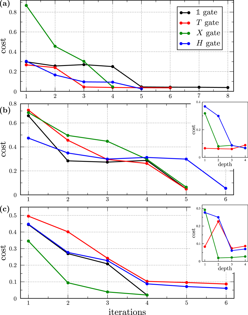
In Fig. 5(a), we show results for compiling single-qubit gates on IBMQX4. All gates (, , , and ) converge to a cost below 0.1, but no gate achieves a cost below our tolerance of . As elaborated upon in Sec. 8, this is due to a combination of finite sampling, gate fidelity, decoherence, and readout error on the device. The single-qubit gates compile to the following gate sequences:
-
1.
gate: , with .
-
2.
gate: , with .
-
3.
gate: .
-
4.
gate: , with .
Figure 5(b) shows results for compiling the same single-qubit gates as above on IBMQX5. The gate sequences have the same structure as listed above for IBMQX4. The optimal angles achieved are for the gate and for the gate. The gate compiles to , and the Hadamard gate compiles to .
In our data collection, we performed on the order of 10 independent optimization runs for each target gate above. The standard deviations of the angles were on the order of , and this can be viewed as the error bars on the average values quoted above.
6.1.2 Rigetti’s quantum computer
The native gate set of Rigetti’s 8Q-Agave 8-qubit quantum computer is
| (34) |
where the single-qubit gates and can be performed on any qubit and the two-qubit CZ gate can be performed between any two qubits allowed in the topology; see [47] for the topology of the 8Q-Agave quantum computer.
As with the implementation on IBM’s quantum computers, for the implementation on Rigetti’s quantum computer we make use of the general procedure outlined in Sec. 3.3. Specifically, we perform random updates to the gate structure followed by continuous optimization over the parameters of the gates using the gradient-free stochastic optimization technique described in Algorithm 1 in Appendix E. In this optimization algorithm, we use fifty cost function evaluations to perform the continuous optimization over parameters. (That is, each iteration in Fig. 5(c) and Fig. 6 uses fifty cost function evaluations, and each cost function evaluation uses calls to the quantum computer for finite sampling.) We take the cost error tolerance (the parameter in Algorithm 1) to be , and for each run of the Hilbert-Schmidt Test, we take samples in order to estimate the cost. Our results are shown in Fig. 5(c). As described in Algorithm 1, we define an iteration to be one accepted update in gate structure followed by a continuous optimization over the internal gate parameters.
The gates compiled in Fig. 5(c) have the following optimal decompositions. The same decompositions also achieve the lowest cost in the cost vs. depth plot in the inset.
-
1.
gate: , with .
-
2.
gate: , with .
-
3.
gate: .
-
4.
gate: , with and .
As with the results on IBM’s quantum computers, none of the gates achieve a cost less than , due to factors such as finite sampling, gate fidelity, decoherence, and readout error. In addition, similar to the IBM results, the standard deviations of the angles here were on the order of , which can be viewed as the error bars on the average values (over 10 independent runs) quoted above.
 denotes the rotation gate , while
  represents the rotation gate .
6.2 Quantum simulator
We now present our results on executing QAQC for single-qubit and two-qubit gates using a simulator. We use the gate alphabet
| (35) |
which is the gate alphabet defined in Eq. (33) except with full connectivity between the qubits. We again use the gradient-free optimization method outlined in Appendix E to perform the continuous parameter optimization. The simulations are performed assuming perfect connectivity between the qubits, no gate errors, and no decoherence.
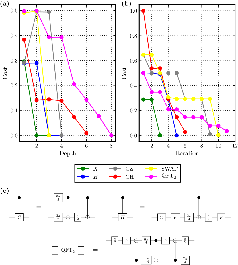
Using Rigetti’s quantum virtual machine [29], we compile the controlled-Hadamard (CH) gate, the CZ gate, the SWAP gate, and the two-qubit quantum Fourier transform by adopting the gradient-free continuous optimization procedure in Algorithm 1. We also compile the single-qubit gates and . For each run of the Hilbert-Schmidt Test to determine the cost, we took samples. Our results are shown in Fig. 6. For the SWAP gate, we find that circuits of depth one and two cannot achieve zero cost, but there exists a circuit with depth three for which the cost vanishes. The circuit achieving this zero cost is the well-known decomposition of the SWAP gate into three CNOT gates. While our compilation procedure reproduces the known decomposition of the SWAP gate, it discovers a decomposition of both the CZ and the gates that differs from their conventional “textbook” decompositions, as shown in Fig. 6(c). In particular, these decompositions have shorter depths than the conventional decompositions when written in terms of the gate alphabet in (35).
In Appendix F, we likewise implement QAQC for one- and two-qubit gates on a simulator, but instead using a gradient-based continuous parameter optimization method outlined therein.
7 Larger-scale implementations
While in the previous section we considered one- and two-qubit unitaries, in this section we explore larger unitaries, up to nine qubits. The purpose of this section is to see how QAQC scales, and in particular, to study the performance of our and cost functions as the problem size increases. We consider two different examples.
Example 1.
In the first example, we let be a tensor product of one-qubit unitaries. Namely we consider
| (36) |
where the are randomly chosen, and is a rotation about the -axis of the Bloch sphere by angle . Similarly, our ansatz for is of the same form,
| (37) |
where the initial values of the angles are randomnly chosen.
Example 2.
In the second example, we go beyond the tensor-product situation and explore a unitary that entangles all the qubits. The target unitary has the form , with
| (38) | ||||
| (39) |
Here, denotes a CNOT with qubit the control and qubit the target, while and are -dimensional vectors of angles. Hence and are layers of CNOTs where the CNOTs in are shifted down by one qubit relative to those in . Our ansatz for the trainable unitary has the same form as but with different angles, i.e., where and are randomly initialized.
In what follows we discuss our implementations of QAQC for these two examples. We first discuss the implementation on a simulator without noise, and then we move onto the implementation on a simulator with a noise model.
7.1 Noiseless implementations
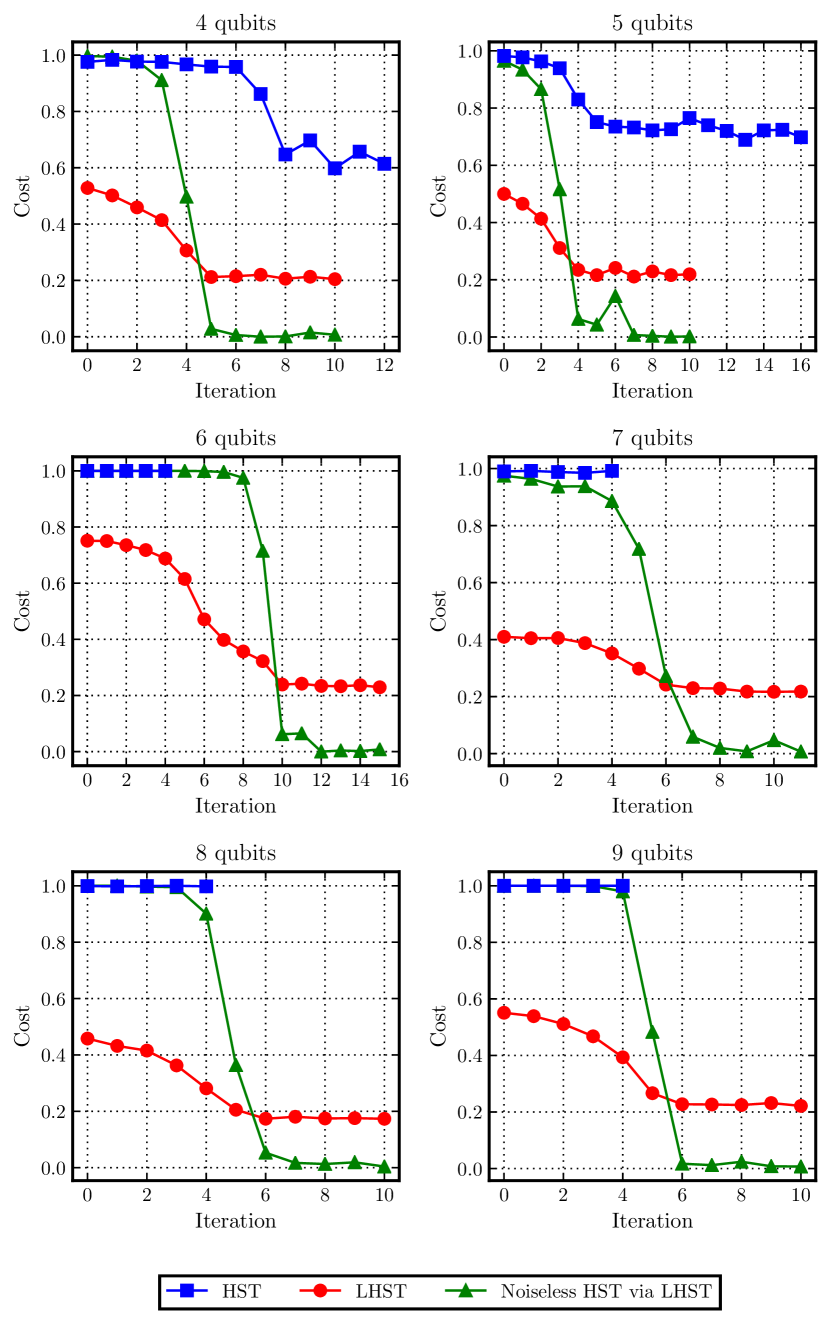
We implemented Examples 1 and 2 on a noiseless simulator. In each case, starting with the ansatz for at a randomly chosen set of angles, we performed the continuous parameter optimization over the angles using a gradient-based approach. We made use of Algorithm 4 in Appendix F.3, which is a gradient descent algorithm that explicitly evaluates the gradient using the formulas provided in Appendix F.3. For each run of the HST and LHST, we took 1000 samples in order to estimate the value of the cost function. The results of this implementation are shown in Figs. 7 and 8.
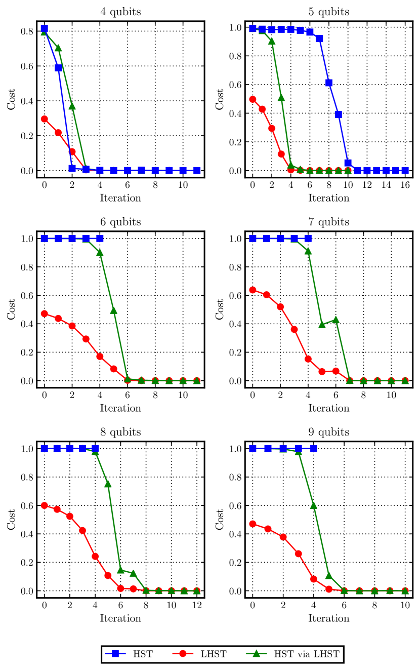
In the case of Example 1 (Fig. 7), both the and cost functions converge to the desired global minimum up to 5 qubits. However, for 6, 7, 8, and 9 qubits, we find cases in which the cost function does not converge to the global minimum but the cost function does. Specifically, the cost stays very close to one, with a gradient value smaller than the pre-set threshold of for four consecutive iterations, causing the gradient descent algorithm to declare convergence. Interestingly, even in the cases that the cost does not converge to the global minimum, training with the cost allows us to fully minimize the cost. (See the green curves labelled “HST via LHST” in Fig. 7, in which we evaluate the cost at the angles obtained during the optimization of the cost.) This fascinating feature implies that, for qubits in Example 1, training our cost is better at minimizing the cost than is directly attempting to train the cost.
7.2 Noisy implementations
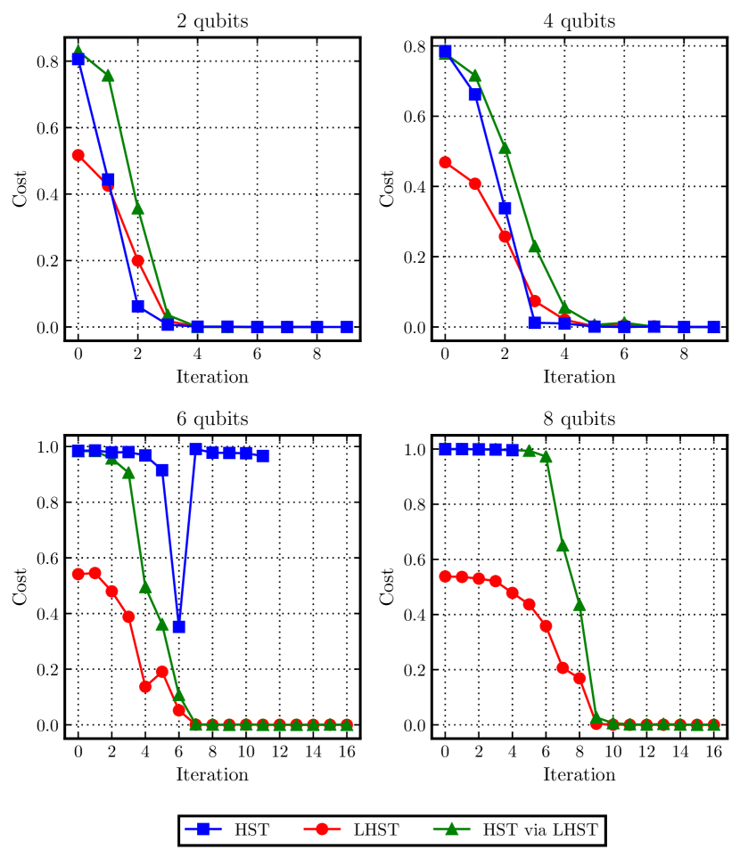
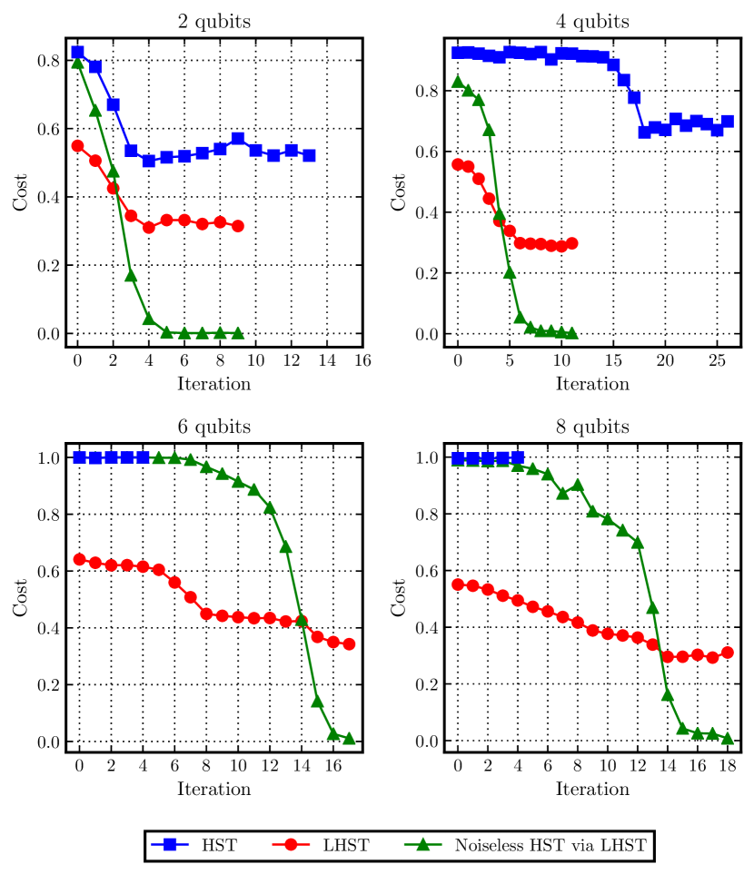
We implemented Examples 1 and 2 on IBM’s noisy simulator, where the noise model matches that of the 16-qubit IBMQX5 quantum computer. This noise model accounts for noise, noise, gate errors, and measurement errors. We emphasize that these are realistic noise parameters since they simulate the noise on currently available quantum hardware. (Note that when our implementations required more than 16 qubits, we applied similar noise parameters to the additional qubits as those for the 16 qubits of the IBMQX5.) We used the same training algorithm as the one we used in the noiseless case above. The results of these implementations are shown in Figs. 9 and 10.
Similar to the noiseless case, for Example 1 (Fig. 9) and for Example 2 (Fig. 10), we find that both the and cost functions converge up to a problem size of 5 qubits. Due to the noise, as expected, both cost functions converge to a value greater than zero. For qubits, however, we find that the cost function does not converge to a local minimum. Specifically, this cost stays very close to one with a gradient value smaller than the pre-set threshold of for four consecutive iterations, causing the gradient descent algorithm to declare convergence. The local cost, on the other hand, converges to a local minimum in every case.
Remarkably, despite the noise in the simulation, we find that the angles obtained during the iterations of the optimization correspond to the optimal angles in the noiseless case. This result is indicated by the green curves labeled “Noiseless HST via LHST”. One can see that the green curves go to zero for the local minima found by training the noisy cost function. Hence, in these examples, training the noisy cost function can be used to minimize the noiseless cost function to the global minimum. This intriguing behavior suggests that the noise has not affected the location (i.e., the value for the angles) of the global minimum. We thus find evidence of the robustness of QAQC to the kind of noise present in actual devices. We elaborate on this point in the next section.
8 Discussion
On both IBM’s and Rigetti’s quantum hardware, we were able to successfully compile one-qubit gates with no a priori assumptions about gate structure or gate parameters. We also successfully implemented QAQC for simple 9-qubit gates on both a noiseless and noisy simulator. These implementations highlighted two important issues, (1) barren plateuas in cost landscape and (2) the effect of hardware noise, which we discuss further now.
8.1 Barren Plateaus
Recent results [48, 49] on gradient-based optimization with random quantum circuits suggest that the probability of observing non-zero gradients tends to become exponentially small as a function of the number of qubits. That work showed that a hardware-efficient ansatz leads to vanishing gradients as the ansatz’s depth becomes deeper (and hence begins to look more like a random unitary). This is an important issue for many variational hybrid algorithms, including QAQC, and motivates the need to avoid a deep, random ansatz. Strategies to address this “barren plateau” issue for QAQC include restricting to a short-depth ansatz, or alternatively employing an application-specific ansatz that takes into account some information about the target unitary . We intend to explore application-specific ansatze in future work to address this issue. There may be other strategies based on the fact that similar issues have been identified in classical deep learning [50]. For instance, recent work [51] shows that gradient descent with momentum (GDM) using an adaptive (multiplicative) integration step update, called resilient backpropagation (rProp), can help with convergence. But, this is an active research area and will likely be important to the success of variational hybrid algorithms.
Interestingly, in this work, we identified another barren plateau issue that is completely independent and distinct from the issue raised in Refs. [48, 49]. Namely, we found that our operationally meaningful cost function, , can have barren plateaus even when the ansatz is a depth-one circuit. The gradient of can vanish exponentially in even when the ansatz has only a single parameter. This issue became apparent in our implementations (see Figs. 7 through 10), where we were unable to directly train the cost for qubits. Fortunately, we fixed this issue by introducing the cost, which successfully trained in all cases we attemped (we attempted up to qubits). Although is not directly operationally meaningful, it is indirectly related to via Eqs. (28) and (29). Hence it can be used to indirectly train , as shown in Figs. 7 through 10. We believe this barren plateau issue will show up in other variational hybrid algorithms. For example, we encountered the same issue in a recently introduced variational algorithm for state diagonalization [52].
8.2 Effect of Hardware Noise
The impact of hardware noise, such as decoherence, gate infidelity, and readout error, is important to consider. This is especially true since QAQC is aimed at being a useful algorithm in the era of NISQ computers, although we remark that QAQC may also be useful for fault-tolerant quantum computing.
On the one hand, we intuitively expect noise to significantly affect the HST and LHST cost evaluation circuits. On the other hand, we see empirical evidence of noise resilience in Figs. 9 and 10. Let us elaborate on both our intuition and our empirical observations now.
A qualitative noise analysis of the HST circuit in Fig. 4(a) is as follows. To compile a unitary acting on qubits, a circuit with qubits is needed. Preparing the maximally-entangled state in the first portion of the circuit requires CNOT gates, which are significantly noisier than one-qubit gates and propagate errors to other qubits through entanglement. In principle, all Hadamard and CNOT gates can be implemented in parallel, but on near-term devices this may not be the case. Additionally, due to limited connectivity of NISQ devices, it is generally not possible to directly implement CNOTs between arbitrary qubits. Instead, the CNOTs need to be “chained” between qubits that are connected, a procedure that can significantly increase the depth of the circuit.
The next level of the circuit involves implementing in the top -qubit register and in the bottom -qubit register. Here, the noise of the computer on is not necessarily undesirable since it could allow us to compile noise-tailored algorithms that counteract the noise of the specific computer, as described in Sec. 2. Nevertheless, the depth of and/or of essentially determines the overall circuit depth as noted in (19), and quantum coherence decays exponentially with the circuit depth. Hence, compiling larger gate sequences involves additional loss of coherence on NISQ computers.
The final level of the HST circuit involves making a Bell measurement on all qubits and is the reverse of the first part of the circuit. As such, the same noise analysis of the first portion of the circuit applies here. Readout errors can be significant on NISQ devices [53], and our HST circuit involves a number of measurements that scales linearly in the number of qubits. Hence, compiling larger unitaries can increase overall readout error.
A similar qualitative noise analysis holds for the LHST circuit in Fig. 4(b), except we note that to calculate the functions in (26) we require only one CNOT gate in the last portion of the LHST circuit before the measurement. Furthermore, we measure only two qubits regardless of the total number of qubits.
With that said, we observed a (somewhat surprising) noise resilience in Figs. 9 and 10. In these implementations, we imported the noise model of the IBMQX5 quantum computer, which is a currently available cloud quantum computer. Hence, we considered realistic noise parameters for decoherence, gate infedility, and readout error. This noise affected all circuit elements of the LHST circuit in Fig. 4(b). Yet we still obtained the correct unitary via QAQC, as shown by the green curves going to zero in Figs. 9 and 10.
Naturally, we plan to investigate this noise resilience in full detail in future work. But it is worth emphasizing the following point here. The value of the cost could be significantly affected by noise without shifting the location of the global minimum in parameter space. In fact, one can see in Figs. 9 and 10 that the value of the cost is significantly affected by noise. Namely, note that the red curves in these plots do not go to zero for larger iterations. However, the green curves do go to zero, which means that QAQC found the correct parameters for despite the noisy cost values.
We could speculate reasons for why the global minimum appears not shift in parameter space with noise. For example, it could be due to the nature of our cost functions. These cost functions can be thought of as entanglement fidelities and hence are related to Hilbert-space averages of input-output fidelities, see Eq. (6). By averaging the input-output fidelity over the whole Hilbert space, the effect of noise could essentially be averaged away. This is just speculation at this point, and we will perform a detailed analysis of the effect of noise in future work. Regardless, our preliminary results in Figs. 9 and 10 suggest that QAQC may indeed be useful in the NISQ era.
9 Conclusions
Quantum compiling is crucial in the era of NISQ devices, where constraints on NISQ computers (such as limited connectivity, limited circuit depth, etc.) place severe restrictions on the quantum algorithms that can be implemented in practice. In this work, we presented a methodology for quantum compilation called quantum-assisted quantum compiling (QAQC), whereby a quantum computer provides an exponential speedup in evaluating the cost of a gate sequence, i.e., how well the gate sequence matches the target. In principle, QAQC should allow for the compiling of larger algorithms than standard classical methods for quantum compiling due to this exponential speedup. As a proof-of-principle, we implemented QAQC on IBM’s and Rigetti’s quantum computers to compile various one-qubit gates to their native gate alphabets. To our knowledge, this is the first time NISQ hardware has been used to compile a target unitary. In addition, we successfully implemented QAQC on a noiseless and noisy simulator for simple 9-qubit unitaries.
Our main technical results were the following. First, we carefully chose a cost function (which involved global and local overlaps between a target unitary and a trainable unitary ) and proved that it satisfied four criteria: it is faithful, it is efficient to compute on a quantum computer, it has an operational meaning, and it scales well with the size of the problem. Second, we presented short-depth circuits (see Sections 4.1 and 4.2) for computing our cost function. Third, we proved that evaluating our cost function is -hard, and hence no classical algorithm can efficiently evaluate our cost function, under reasonable complexity assumptions. This established a rigorous proof for the difficulty of classically simulating QAQC. We also remark that, in the Appendix, we detailed our gradient-free and gradient-based methods for optimizing our cost function. This included a circuit for gradient computation that generalizes the famous Power of One Qubit [26] and hence is likely of interest to a broader community.
As elaborated in the Discussion section, our noisy implementations of QAQC showed a surprising resilience to noise. While simulating realistic noise parameters based on a currently available cloud quantum computer (IBMQX5), we were able to run QAQC on a 9-qubit unitary and obtain the correct parameters for . We plan to investigate this intriguing noise resilience in future work.
QAQC is a novel variational hybrid algorithm, similar to other well-known variational hybrid algorithms such as VQE [18] and QAOA [2]. Variational hybrid algorithms are likely to provide some of the first real applications of quantum computers in the NISQ era. In the case of QAQC, it is an algorithm that makes other algorithms more efficient to implement, via algorithm depth compression. We note that the ability to compress algorithm depth will also be useful (to reduce the run-time of quantum circuits) in the era of fault-tolerant quantum computing. The central application of QAQC is thus to make quantum computers more useful.
Acknowledgements
We thank IBM and Rigetti for providing access to their quantum computers. The views expressed in this paper are those of the authors and do not reflect those of IBM or Rigetti. SK, RL, and AP acknowledge support from the U.S. Department of Energy through a quantum computing program sponsored by the LANL Information Science & Technology Institute. RL acknowledges support from an Engineering Distinguished Fellowship through Michigan State University. AP is partially supported by AFOSR YIP award number FA9550-16-1-0495 and the Institute for Quantum Information and Matter, an NSF Physics Frontiers Center (NSF Grant PHY-1733907) and the Kortschak Scholars program. LC was supported by the U.S. Department of Energy through the J. Robert Oppenheimer fellowship. ATS and PJC were supported by the LANL ASC Beyond Moore’s Law project. LC, ATS, and PJC were also supported by the LDRD program at LANL. We thank Alexandru Gheorghiu and Thomas Vidick for useful discussions.
References
- Shor [1997] P. Shor, Polynomial-time algorithms for prime factorization and discrete logarithms on a quantum computer, SIAM Journal on Computing 26, 1484 (1997).
- Farhi et al. [2014] E. Farhi, J. Goldstone, and S. Gutmann, A quantum approximate optimization algorithm, arXiv:1411.4028 (2014).
- Feynman [1982] R. P. Feynman, Simulating physics with computers, International Journal of Theoretical Physics 21, 467 (1982).
- Preskill [2018] J. Preskill, Quantum computing in the NISQ era and beyond, Quantum 2, 79 (2018).
- Preskill [2012] J. Preskill, Quantum computing and the entanglement frontier, arXiv:1203.5813 (2012).
- Neill et al. [2018] C. Neill, P. Roushan, K. Kechedzhi, S. Boixo, S. V. Isakov, V. Smelyanskiy, et al., A blueprint for demonstrating quantum supremacy with superconducting qubits, Science 360, 195 (2018).
- Venturelli et al. [2018] D. Venturelli, M. Do, E. Rieffel, and J. Frank, Compiling quantum circuits to realistic hardware architectures using temporal planners, Quantum Science and Technology 3, 025004 (2018).
- Booth et al. [2018] K. E. C. Booth, M. Do, J. C. Beck, E. Rieffel, D. Venturelli, and J. Frank, Comparing and integrating constraint programming and temporal planning for quantum circuit compilation, arXiv:1803.06775 (2018).
- Cincio et al. [2018] L. Cincio, Y. Subaşı, A. T. Sornborger, and P. J. Coles, Learning the quantum algorithm for state overlap, New Journal of Physics 20, 113022 (2018).
- Maslov et al. [2008] D. Maslov, G. W. Dueck, D. M. Miller, and C. Negrevergne, Quantum circuit simplification and level compaction, IEEE Transactions on Computer-Aided Design of Integrated Circuits and Systems 27, 436 (2008).
- Fowler [2011] A. G. Fowler, Constructing arbitrary Steane code single logical qubit fault-tolerant gates, Quantum Information and Computation 11, 867 (2011).
- Booth Jr [2012] J. Booth Jr, Quantum compiler optimizations, arXiv:1206.3348 (2012).
- Nam et al. [2018] Y. Nam, N. J. Ross, Y. Su, A. M. Childs, and D. Maslov, Automated optimization of large quantum circuits with continuous parameters, npj Quantum Information 4, 23 (2018).
- Chong et al. [2017] F. T. Chong, D. Franklin, and M. Martonosi, Programming languages and compiler design for realistic quantum hardware, Nature 549, 180 (2017).
- Heyfron and Campbell [2018] L. E. Heyfron and E. T. Campbell, An efficient quantum compiler that reduces T count, Quantum Science and Technology 4, 015004 (2018).
- Häner et al. [2018] T. Häner, D. S. Steiger, K. Svore, and M. Troyer, A software methodology for compiling quantum programs, Quantum Science and Technology 3, 020501 (2018).
- Oddi and Rasconi [2018] A. Oddi and R. Rasconi, in International Conference on the Integration of Constraint Programming, Artificial Intelligence, and Operations Research (Springer, 2018) pp. 446–461.
- Peruzzo et al. [2014] A. Peruzzo, J. McClean, P. Shadbolt, M.-H. Yung, X.-Q. Zhou, P. J. Love, A. Aspuru-Guzik, and J. L. O’Brien, A variational eigenvalue solver on a photonic quantum processor, Nature Communications 5, 4213 (2014).
- Johnson et al. [2017] P. D. Johnson, J. Romero, J. Olson, Y. Cao, and A. Aspuru-Guzik, QVECTOR: an algorithm for device-tailored quantum error correction, arXiv:1711.02249 (2017).
- Benedetti et al. [2018a] M. Benedetti, D. Garcia-Pintos, O. Perdomo, V. Leyton-Ortega, Y. Nam, and A. Perdomo-Ortiz, A generative modeling approach for benchmarking and training shallow quantum circuits, arXiv:1801.07686 (2018a).
- Mitarai et al. [2018] K. Mitarai, M. Negoro, M. Kitagawa, and K. Fujii, Quantum circuit learning, Physical Review A 98, 032309 (2018).
- Verdon et al. [2018] G. Verdon, J. Pye, and M. Broughton, A Universal Training Algorithm for Quantum Deep Learning, arXiv:1806.09729 (2018).
- Romero et al. [2017] J. Romero, J. P. Olson, and A. Aspuru-Guzik, Quantum autoencoders for efficient compression of quantum data, Quantum Science and Technology 2, 045001 (2017).
- Romero et al. [2018] J. Romero, J. P. Olson, and A. Aspuru-Guzik, Quantum autoencoders for short depth quantum circuit synthesis, GitHub article (2018).
- Dive et al. [2018] B. Dive, A. Pitchford, F. Mintert, and D. Burgarth, In situ upgrade of quantum simulators to universal computers, Quantum 2, 80 (2018).
- Knill and Laflamme [1998] E. Knill and R. Laflamme, Power of one bit of quantum information, Physical Review Letters 81, 5672 (1998).
- Fujii et al. [2018] K. Fujii, H. Kobayashi, T. Morimae, H. Nishimura, S. Tamate, and S. Tani, Impossibility of Classically Simulating One-Clean-Qubit Model with Multiplicative Error, Physical Review Letters 120, 200502 (2018).
- Rosgen and Watrous [2005] B. Rosgen and J. Watrous, in 20th Annual IEEE Conference on Computational Complexity (CCC’05) (2005) pp. 344–354.
- Smith et al. [2016] R. S. Smith, M. J. Curtis, and W. J. Zeng, A practical quantum instruction set architecture, arXiv:1608.03355 (2016).
- Cross et al. [2017] A. W. Cross, L. S. Bishop, J. A. Smolin, and J. M. Gambetta, Open Quantum Assembly Language, arXiv:1707.03429 (2017).
- Nielsen and Chuang [2000] M. A. Nielsen and I. L. Chuang, Quantum Computation and Quantum Information (Cambridge University Press, 2000).
- Kitaev [1997] A. Kitaev, Quantum computations: algorithms and error correction, Russian Mathematical Surveys 52, 1191 (1997).
- Dawson and Nielsen [2006] C. M. Dawson and M. A. Nielsen, The Solovay-Kitaev algorithm, Quantum Information and Compututation 6, 81 (2006).
- Pham et al. [2013] T. T. Pham, R. Van Meter, and C. Horsman, Optimization of the Solovay-Kitaev algorithm, Physical Review A 87, 052332 (2013).
- Kliuchnikov et al. [2013] V. Kliuchnikov, D. Maslov, and M. Mosca, Asymptotically optimal approximation of single qubit unitaries by Clifford and T circuits using a constant number of ancillary qubits, Physical Review Letters 110, 190502 (2013).
- Kliuchnikov et al. [2014] V. Kliuchnikov, A. Bocharov, and K. M. Svore, Asymptotically optimal topological quantum compiling, Physical Review Letters 112, 140504 (2014).
- Zhiyenbayev et al. [2018] Y. Zhiyenbayev, V. M. Akulin, and A. Mandilara, Quantum compiling with diffusive sets of gates, Physical Review A 98, 012325 (2018).
- Horodecki et al. [1999] M. Horodecki, P. Horodecki, and R. Horodecki, General teleportation channel, singlet fraction, and quasidistillation, Physical Review A 60, 1888 (1999).
- Nielsen [2002] M. A. Nielsen, A simple formula for the average gate fidelity of a quantum dynamical operation, Physics Letters A 303, 249 (2002).
- Gepp and Stocks [2009] A. Gepp and P. Stocks, A review of procedures to evolve quantum algorithms, Genetic Programming and Evolvable Machines 10, 181 (2009).
- Suzuki [1990] M. Suzuki, Fractal decomposition of exponential operators with applications to many-body theories and monte carlo simulations, Physics Letters A 146, 319 (1990).
- Jones and Benjamin [2018] T. Jones and S. C. Benjamin, Quantum compilation and circuit optimisation via energy dissipation, arXiv:1811.03147 (2018).
- Garcia-Escartin and Chamorro-Posada [2013] J. C. Garcia-Escartin and P. Chamorro-Posada, Swap test and Hong-Ou-Mandel effect are equivalent, Physical Review A 87, 052330 (2013).
- Shor and Jordan [2008] P. W. Shor and S. P. Jordan, Estimating jones polynomials is a complete problem for one clean qubit, Quantum Information & Computation 8, 681 (2008).
- IBM [2018a] IBM Q 5 Tenerife backend specification, (2018a).
- IBM [2018b] IBM Q 16 Rueschlikon backend specification, (2018b).
- rig [2018] Rigetti 8Q-Agave specification v.2.0.0.dev0, (2018).
- McClean et al. [2018] J. R. McClean, S. Boixo, V. N. Smelyanskiy, R. Babbush, and H. Neven, Barren plateaus in quantum neural network training landscapes, Nature Communications 9, 4812 (2018).
- Day et al. [2019] A. G. R. Day, M. Bukov, P. Weinberg, P. Mehta, and D. Sels, Glassy phase of optimal quantum control, Physical Review Letters 122, 020601 (2019).
- Glorot and Bengio [2010] X. Glorot and Y. Bengio, in In Proceedings of the International Conference on Artificial Intelligence and Statistics (2010) pp. 249–256.
- Benedetti et al. [2018b] M. Benedetti, D. Garcia-Pintos, O. Perdomo, V. Leyton-Ortega, Y. Nam, and A. Perdomo-Ortiz, A generative modeling approach for benchmarking and training shallow quantum circuits, arXiv:1801.07686 (2018b).
- LaRose et al. [2018] R. LaRose, A. Tikku, É. O’Neel-Judy, L. Cincio, and P. J. Coles, Variational quantum state diagonalization, arXiv:1810.10506 (2018).
- Kandala et al. [2018] A. Kandala, K. Temme, A. D. Corcoles, A. Mezzacapo, J. M. Chow, and J. M. Gambetta, Extending the computational reach of a noisy superconducting quantum processor, Nature 567, 491 (2018).
- sci [2018a] Scikit-optimize, (2018a).
- Močkus [1975] J. Močkus, in Optimization Techniques IFIP Technical Conference Novosibirsk, July 1–7, 1974 (Springer Berlin Heidelberg, Berlin, Heidelberg, 1975) pp. 400–404.
- Osborne et al. [2009] M. A. Osborne, R. Garnett, and S. J. Roberts, in 3rd International Conference on Learning and Intelligent Optimization (LION3) 2009 (2009).
- Rebentrost et al. [2016] P. Rebentrost, M. Schuld, L. Wossnig, F. Petruccione, and S. Lloyd, Quantum gradient descent and Newton’s method for constrained polynomial optimization, arXiv:1612.01789 (2016).
- Kerenidis and Prakash [2017] I. Kerenidis and A. Prakash, Quantum gradient descent for linear systems and least squares, arXiv:1704.04992 (2017).
- [59] A. Gilyén, S. Arunachalam, and N. Wiebe, Optimizing quantum optimization algorithms via faster quantum gradient computation, in Proceedings of the Thirtieth Annual ACM-SIAM Symposium on Discrete Algorithms, pp. 1425–1444.
- Sousa and Ramos [2007] P. B. M. Sousa and R. V. Ramos, Universal quantum circuit for -qubit quantum gate: A programmable quantum gate, Quantum Information and Computation 7, 228 (2007).
- Vatan and Williams [2004] F. Vatan and C. Williams, Optimal quantum circuits for general two-qubit gates, Physical Review A 69, 032315 (2004).
- sci [2018b] Scipy optimization and root finding, (2018b).
- Zhou et al. [2011] X.-Q. Zhou, T. C. Ralph, P. Kalasuwan, M. Zhang, A. Peruzzo, B. P. Lanyon, and J. L. O’Brien, Adding control to arbitrary unknown quantum operations, Nature Communications 2, 413 (2011).
Appendix A Remark on implementation of
As mentioned in Sec. 4, a subtle point about evaluating the cost functions and is that the complex conjugate must be executed on the quantum computer, not itself. The complex conjugate of a unitary corresponding to a gate sequence can be obtained by taking the complex conjugate of each unitary in the gate sequence. However, if each gate in the sequence comes from a gate alphabet , it is possible that the complex conjugate of a gate in the sequence is not contained in the alphabet; for example, if , then the complex conjugate of , which is , is not contained in . But the unitary is equal (up to a global phase) to . There are thus two ways to proceed when performing the compilation procedure: during the optimization over the continuous parameters, directly run the gate sequence corresponding to , expressing it in terms of the native gate alphabet of the quantum computer, then at the end establish the complex conjugate of the optimal unitary as the unitary to which has been compiled. This would involve translating the complex conjugate of each gate in the optimal sequence into the native gate alphabet of the quantum computer. An alternative is to first take the complex conjugate by translating the complex conjugate of each gate in the sequence into the native gate alphabet, then execute the resulting sequence on the quantum computer. In each case, we allow for a small-scale classical compiler that can perform the simple translation of the complex conjugate of a gate sequence into the native gate alphabet of the quantum computer. Note that this small-scale classical compiler does not come with exponential overhead because it is only compiling one- and two-qubit gates.
Also, observe that if a gate alphabet is not closed under complex conjugation, then the depth of a gate sequence from that alphabet can increase by taking its complex conjugate. This is true for the example given above, in which the complex conjugate of has a depth of three under the alphabet , while the original gate has a depth of only one. However, in general, note that the final depth increases by at most a constant factor relative to the original depth.
Appendix B Faithfulness of LHST cost function
See 1
Proof: First, we note that since for all , we get that if and only if , i.e., , for all . Next, since is by definition the entanglement fidelity of the channel , we have that if and only if is the identity channel . Finally, the condition is equivalent to . Therefore, it suffices to prove that if and only if is the identity channel for all . The implication for all is immediate. We now prove the converse.
Let , and suppose that has the following operator Schmidt decomposition under the bipartite cut :
| (40) |
where and are orthonormal sets of operators, are the Schmidt coefficients of , and is the Schmidt rank of . Since is unitary, we have
| (41) |
which implies that
| (42) |
Plugging in the Schmidt decomposition of into the definition of in (24), we get
| (43) |
The operators can therefore be regarded as Kraus operators for . Indeed, they satisfy the following condition for trace preservation:
| (44) | ||||
| (45) | ||||
| (46) |
where to obtain the second equality we used (42).
Now, we assume that is the identity channel, meaning that for all states . By the non-uniqueness of Kraus representations of quantum channels, there exists an isometry relating the Kraus operators to another set of Kraus operators according to . Since one Kraus representation of the identity channel is the one consisting of only the identity operator , we let the set consist of only the identity operator. The isometry is then a matrix, so that for all . This implies that for all . Therefore,
| (47) | ||||
| (48) | ||||
| (49) | ||||
| (50) |
where in the last line we have defined the unitary .
Now, given the assumption that , so that has the form in (50), we get that
| (51) |
Therefore, applying the procedure above for by taking the bipartite cut in the operator Schmidt decomposition of to be , we get that if is the identity channel, then for some unitary acting on . Continuing in this manner for all up to , assuming in each case that is the identity channel, we ultimately obtain , which implies that , as required.
Appendix C Relation between and
See 2
Proof: First we rewrite the global cost function:
| (52) | ||||
where . Also, for the local cost function, we have
| (53) |
where
| (54) | ||||
and we have defined
| (55) |
which are projectors that all mutually commute. Let
| (56) |
Then, we can write as
| (57) |
and we can write as
| (58) |
for all . If we associate the events with the projectors , so that , then, .
To prove (28), namely , we recall a basic inequality in probability theory. For any set of events, it holds that
| (59) |
Let us take in (59). Then,
| (60) | ||||
| (61) |
By definition of the events , the last equality is precisely , as required.
To prove (29), we make use of the union bound:
| (62) | ||||
| (63) | ||||
| (64) |
Given that the left-hand side of the above inequality is precisely , we have that , as required.
Appendix D Proofs of complexity theorems
See 1
Proof: We show that the problem of approximating the cost is hard for . In other words, we have to show that any problem in reduces to an instance of approximating for some . Recall that, given as input a -sized unitary on -qubits, any problem in requires us to estimate the acceptance probability when measuring the outcome “” on input , i.e.
| (65) |
Note that, since the above equation describes a probability via the positive semi-definite operator , the trace will result in a non-negative real number. Let us re-write Eq. (65) as follows:
| (66) |

When letting as in Fig. 11, we can also write
| (67) |
hence the problem is equivalent to approximating the absolute value of the trace of a unitary . In fact, given our choice of and when taking to be the identity, the problem reduces to an instance of approximating the cost up to some precision via a simple reduction. Therefore, we have shown that the problem of approximating up to -precision is -hard.
See 2
Proof: We show that any problem in reduces to an instance of approximating via a reduction. We are given as input a -sized unitary on -qubits, and the task is to estimate the acceptance probability of outputting . Our proof strategy is to show that one can efficiently extract , the trace of an -qubit unitary , from two distinct evaluations of and elementary post-processing. This implies that computing is hard for , since all problems in can be seen as estimating the real part of via Eq. (66) and Eq. (67).
The two cost function evaluations that we consider are and , where
| (68) | ||||
| (69) |
Here, denotes controlled- operation.
First, consider and let the qubit correspond to the control qubit for the controlled unitary. Then one can show that
| (70) | ||||
| (71) |
This gives
| (72) |
For notational simplicity, let . Then, we can rewrite Eqs. (D) as
| (73) |
Hence, we have that
| (74) |
By choosing according to Fig. 11, one can see from Eq. (66) and Eq. (67) that the problem is equivalent to -approximating our local cost function for some . Hence, any problem can be efficiently solved for by computing a simple linear combination of two instances of . Therefore, we have shown that the problem of approximating the cost is hard for .
Appendix E Gradient-free optimization method
We now outline our approach to gradient-free optimization of over the continuous gate parameters in the trainable unitary . This approach was used to obtain the results in Sec. 6. Given that this is an implementation for small problem size, we employ the cost function . However, we note that one can replace with our general cost function for larger problem sizes.
Optimization for QAQC via the HST
Recall that we compute the cost function using the Hilbert-Schmidt Test (HST), as described in Sec. 4.1 and illustrated in Fig. 4(a). For a given set of gate structure parameters , the calculation of the cost on a quantum computer (as well as on a simulator) is affected by the fact that, due to finite sampling, the HST allows us to obtain only an estimate of the magnitude of the Hilbert-Schmidt inner product. Noise within the quantum computer itself also affects the calculation of the cost. Therefore, in order to perform gradient-free optimization over the continuous gate parameters , we make use of stochastic optimization techniques that are designed to optimize noisy functions. Specifically, we make use of the gp_minimize routine in the scikit-optimize Python library [54], which is a gradient-free optimization routine that performs Bayesian optimization using Gaussian processes [55, 56]. See Algorithm 1 for a general overview of the optimization procedure. Note that with this algorithm, we obtain an -approximate compilation of , with
| (75) |
In the small-scale quantum computer implementations of Fig. 5(c) and Fig. 6, we use 50 objective function evaluations in gp_minimize per iteration. Note that evaluating the objective function involves running the quantum circuit many times in order to sample from the output distribution of the circuit.
For large problem sizes, as described in Sec. 3.4, we propose using the cost function . The gradient-free continuous parameter optimization algorithm for is similar to the one for in Algorithm 1, except that in addition to running the HST we run the LHST for every qubit in order to compute the local cost . In this case, the algorithm provides an -approximate compilation of , with
| (76) |
We emphasize that our approach to gradient-free optimization avoids the exponential overhead of evaluating the cost function classically, yet at the same time makes use of fast and efficient classical heuristics for optimization. In fact, using the HST, Algorithm 1 requires only calls to the quantum computer in order to evaluate the cost, where is the sample precision, which is related to the number of samples taken from the device.
E.1 Alternative method for gradient-free optimization
Here we propose an alternative algorithm for gradient-free optimization that, on average, significantly reduces the number of times the objective function is evaluated. As a result, it is more suitable for cloud computing under a queue submission system (e.g., IBM’s Quantum Experience). This algorithm performs a “multi-scale bisection” of the parameter space based on simulated annealing. We implement this method in Sec. 6.1.1 specifically for the hardware of IBM because the queue submission system can require a significant amount of time to make many calls to the quantum computer.
This alternative approach to performing gradient-free continuous parameter optimization is outlined in Algorithm 2. We start with four angles spread uniformly in the interval —namely and . This significantly reduces the size of the search space and allows us to get close to, or find exactly, an optimal gate sequence. Once the optimal structure is reached from this step, we then bisect the angles for each gate by evaluating the cost with a new circuit containing , where is determined by the iteration in the procedure. Although we do not explore all angles in the interval, the runtime is logarithmically faster than a continuous search due to the bisection procedure. An additional advantage of this approach is that many gates have angles that are simple fractions of , e.g., and .
In a noiseless environment, the two steps above are sufficient. On actual devices, we implement a third step of stochastic optimization by evaluating the cost for the new circuit with each gate replaced by for some small value decreasing monotonically with the iteration . This allows us to compile for a given device by accounting for noise and gate errors. This can be thought of as a “fine-grained” angular optimization in contrast to the previous “coarse-grained” angular optimization.
using Bisection for QAQC
Appendix F Gradient-based optimization method
We now describe a gradient-based approach to performing the optimization over the continuous parameters in the trainable gate sequence . In Sec. F.1, we define a new cost function for this purpose, and we introduce a quantum circuit to calculate this cost function on a quantum computer. In Sec. F.2, we present the results of implementing this method on a quantum simulator. In Sec. F.3, we briefly describe how the original cost functions and can also be optimized using a gradient-based method.
While recent work on gradient descent continuous optimization has shown vast quantum speedups over classical variants [57, 58, 59], the majority of proposals still appear to be out of reach for implementations on NISQ devices, mainly due to their use of certain algorithmic techniques, such as quantum random-access memory, the quantum Fourier transform, and the Grover search algorithm, which have high resource requirements. Instead, we focus on continuous optimization procedures that are feasible on current quantum computers and leave improvements to our algorithms as an open problem.
The gradient with respect to of the gate sequence given by
| (77) |
is defined by
| (78) |
where the matrix element of the -th component is
| (79) |
For example, consider the rotation gate , which is parametrized by the angle . Then, the derivative with respect to can be written as
| (80) |
which follows from the Taylor series expansion of the exponent.
Now, evaluating the gradient on a quantum computer is possible due to the fact that for the gate alphabets we consider in this paper, only the single-qubit gates are parameterized, and these gates are simply rotation gates. In fact, any unitary gate can be decomposed into circuits in which only the single-qubit rotation gates are present. This is illustrated in Fig. 12. Furthermore, the circuits in Fig. 12(a) and Fig. 12(b) are universal for one- and two-qubit gates, respectively (see [60], which also contains universal circuits for -qubit gates). This means that our gradient-based approach can be applied to any -qubit unitary without explicitly searching over gate structures, though the compilations obtained in this manner will generally have sub-optimal depth.

F.1 The Power of Two Qubits
Consider the following cost function based on the normalized Hilbert-Schmidt distance between the unitaries and :
| (81) | ||||
where POTQ stands for “Power of Two Qubits” and refers to the circuit used to evaluate it, which we present below. Note that is zero if and only if . Contrary to the cost function , which is defined using the magnitude of the inner product , this cost function is defined using the real part of the inner product. Consequently, it does not vanish if and differ only by a global phase. Indeed, if , then .
Before discussing the circuit used to evaluate the cost function , let us review the Power of One Qubit (POOQ) [26], shown in Fig. 13(a), which is a circuit for computing the trace of a -dimensional unitary . This circuit acts on a -dimensional system , initially in the maximally mixed state, , and on a single-qubit ancilla initially in the state. After applying a Hadamard gate to and a controlled- gate to (with the control system), the reduced density matrix has its off-diagonal elements proportional to . Hence, one can measure in the and bases, respectively, to read off the real and imaginary parts of .
We now introduce a circuit for computing the real and imaginary parts of that generalizes the POOQ and is called the Power of Two Qubits (POTQ), depicted in Fig. 13(b). As the name suggests, the POTQ employs two single-qubit ancillas, and , each initially in the state. In addition, two -dimensional systems, and , are initially prepared in the Bell state defined in Eq. (14). (Although not shown in Fig. 13(b), this Bell state is prepared with a depth-two circuit, as shown in Fig. 4.)
The first step in the POTQ is to prepare the two-qubit maximally entangled state between and , using the Hadamard and CNOT gates as shown in Fig. 13(b). The second step is to apply a controlled- gate between and (with the control system). In parallel with this gate, the anticontrolled- gate is applied to , with the control system, where anticontrolled means that the roles of the and states on the control system are reversed in comparison to a controlled gate. This results in the state:
| (82) |
where to obtain the equality we used the ricochet property in Eq. (18). As in the HST, note that itself is not implemented. In this case, its transpose is implemented.
Finally, a CNOT gate is applied to , with the control system. This results in the reduced state on being
| (83) |
By inspection of , one can see that measuring in the and bases, respectively, gives the real and imaginary parts of .
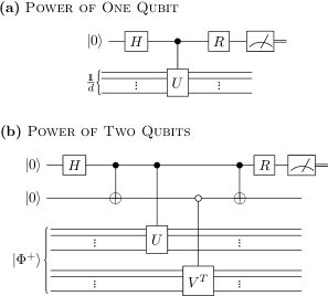
Interestingly, if we set to the identity in the POTQ, then since the CNOT gate commutes with the controlled- gate and the reduced state of is the maximally mixed state , we recover the POOQ. The POTQ is therefore a generalization of the POOQ.
Note that while the POOQ can also be used to determine , the POTQ has the advantage that the controlled gates for and can be executed in parallel, while in the POOQ they would have to be executed in series. This makes the POTQ better suited for NISQ devices, where short depth is crucial. Consider the depth of the POTQ. Denoting the controlled- and the anticontrolled- as and respectively, the overall depth is
| (84) |
Note the similarity here to Eq. (19). The overall depth is essentially determined by whichever controlled gate has the largest depth.
F.2 Gradient-based optimization via the POTQ
The gradient with respect to of can be computed using the POTQ. This is due to the fact that
| (85) |
where
| (86) | ||||
is the original gate sequence except with an additional Pauli gate corresponding to the variable with respect to which the derivative is taken. (Note that for the gate alphabets that we consider in this paper, only the single-qubit gates are parameterized, and these gates are simply rotation gates. The derivative of any one-qubit rotation gate is analogous to the expression in (80) for the derivative of the rotation gate .) This means that to compute the gradient of , we simply add the appropriate local Pauli gate to the original gate sequence and run the POTQ on this new gate sequence.
Optimization for QAQC via the POTQ
Our gradient-based optimization procedure is outlined in Algorithm 3. Given an arbitrary unitary as input, Algorithm 3 compiles to a unitary of a given structure that minimizes the cost . The gradient is evaluated with the POTQ circuit as a subroutine within a classical gradient-descent algorithm. The overall query complexity in the number of calls to the cost evaluation routine of Algorithm 3 is , where is the sample precision, is the maximum number of repetitions over random initial parameters , is the dimension of the continuous parameter space of , and is the number of gradient descent iterations for a suitable learning rate . In order to improve convergence, it may also be useful to supply the quantum subroutines for computing the cost function and the gradient to a more advanced minimization routine, for example as found in the Python library SciPy [62]. We present below the results on compiling both single-qubit and two-qubit gates on a simulator.
When performing Algorithm 3, we rely on the ability to perform the controlled- gate. The unitary may be unknown, e.g., as in Fig. 1(b). In general, to perform a controlled operation with respect to a target unitary , one can use a method for “remote control” [63]. This method employs a local gate and controlled-SWAP operations in order to realize the controlled- gate. In practice, since any controlled unitary gate can be decomposed into native gates, the ability to compile controlled-SWAP, the Toffoli gate, and the set of controlled rotations is sufficient. In order to perform such a translation, we allow the user to have access to a small-scale classical compiler. This does not incur exponential overhead since the gates to be translated are one- and two-qubit gates (or their controlled versions). While this may cause the depth of our compiled unitary to increase, it will only be by a constant factor.
We note that decoherence, gate infidelity, and readout errors on NISQ computers are all more pronounced when attempting to execute controlled unitaries. This means that there is significant performance loss for controlled unitaries, as required in the POTQ. Consequently, we did not implement our gradient-based optimization method on current quantum devices, but we speculate that improvements to quantum hardware will enable this application.
F.2.1 Implementation on a quantum simulator

We use IBM’s simulator [30] to compile a selection of single-qubit and two-qubit gates by performing the gradient-based optimization procedure in Algorithm 3. In order to improve convergence, we additionally supply the gradient, as well as the cost function, to the minimize routine in the SciPy-optimize Python library [62]. For the single-qubit gates, we assume a fixed structure for the trainable gate sequence according to the decomposition in Fig. 12(a), while for the two-qubit gates we assume a fixed structure for the trainable gate sequence according to the decomposition in Fig. 12(b). We compile the gate, gate, Hadamard () gate, as well as the CNOT and CZ gates, all with . The results are shown in Fig. 14. We note that increasing to higher orders of magnitude significantly reduces the sampling error and results in more stable convergence at the cost of an increase in runtime.
F.3 Gradient-based optimization via the HST and LHST
We now show that it is possible to perform gradient-based optimization of the original cost function and its local variant . This allows us to perform gradient-based optimization of the general cost function . The algorithm for gradient-based optimization of and is presented in Algorithm 4.
The gradient with respect to of both and can be computed using the HST and the LHST, respectively. Specifically, for a gate sequence of the form in (77), in which the only parameterized gates are the single-qubit rotation gates, we have that
| (87) | ||||
and
| (88) | ||||
for all . Here,
| (89) | ||||
is the original gate sequence with an additional rotation gate corresponding to the variable with respect to which the derivative is taken. In other words, to compute the gradient of the cost function , we run the HST in Fig. 4(a) twice, once with the gate sequence and once with the gate sequence . Similarly, to compute the gradient of the functions , we run the LHST in Fig. 4(b) twice, once with the gate sequence and once with the gate sequence .
The expressions for the gradient in (87) and (88) can be verified by recalling that only the one-qubit gates need to be parameterized and that they can always be assumed to have the form for some Pauli operator , where is the continuous parameter specifying the gate. Then, for the gate sequence in (77), we get
| (90) | ||||
| (91) |
Then, we use the identity
| (92) | ||||
which holds for any state . We also observe that both the functions and are of the form
| (93) |
where for both functions, for , and for . Finally, using
| (94) |
substituting (91) into this expression, and using (92) to simplify, we obtain (87) and (88).
Optimization for QAQC via the HST and LHST