Conditional channel simulation

Abstract

In this work we design a specific simulation tool for quantum channels which is based on the use of a control system. This allows us to simulate an average quantum channel which is expressed in terms of an ensemble of channels, even when these channel-components are not jointly teleportation-covariant. This design is also extended to asymptotic simulations, continuous ensembles, and memory channels. As an application, we derive relative-entropy-of-entanglement upper bounds for private communication over various channels, including non-Gaussian mixtures of bosonic lossy channels. Among other results, we also establish the two-way quantum and private capacity of the so-called “dephrasure” channel.

I Introduction

In quantum information theory Hayashi ; first , the simulation of quantum channels has a long history which dates back to 1996 BDSW soon after the introduction of the teleportation protocol tele ; telereview . Indeed the first idea of simulating a Pauli channel by teleporting over a two-qubit mixed state was re-visited in various papers (e.g., see Ref. followPauli ). The most general formulation of channel simulation based on local operation and classical communication (LOCC) has been given in Ref. PLOB and allows one to simulate both discrete- and continuous-variable channels RMP . This is also known as LOCC-simulation of a quantum channel (see Ref. (TQC, , Sec. 9) for a detailed review on the topic).

Similar ideas were put forward by Nielsen and Chuang Array in the context of discrete-variable quantum computing. Ref. Array introduced the notion of quantum programmable gate array (QPGA) where a channel $\mathcal{E}$ is simulated by inserting its input $\rho$ and a program state $\sigma$ into a universal unitary operation $G$ so that $\mathcal{E}(\rho)=\mathrm{Tr}_{\text{prog}}[G(\sigma_{\text{prog}}\otimes\rho)]$. For an arbitrary channel $\mathcal{E}$ this is always possible as long as the operation $G$ can be performed over arbitrarily many ancillary systems (i.e., arbitrarily large programs). This can also be understood in the context of port-based teleportation (PBT) PBT ; PBT1 ; PBT2 ; PBT2bis ; PBT3 , which allows for perfect simulations in the limit of many ports. Indeed, PBT not only provides a design for the QPGA but also shows that it can be based on a teleportation-like LOCC, with various implications for quantum and private communications PBT3 .

The applications of channel simulations are various. One of the most important is certainly the simplification of adaptive (i.e., feedback-based) quantum protocols into corresponding block (i.e., non feedback) versions. This is achieved by replacing the channels with their simulations and to apply a suitable re-organization of the adaptive operations of the protocol, in such a way to decompose the output state into a tensor product of program states up to a single quantum operation. This adaptive-to-block reduction is also known as (teleportation) stretching of the protocol PLOB and can be applied to both discrete- and continuous-variable settings (see Ref. TQC for a review of the various techniques of adaptive-to-block reduction). Combining teleportation stretching with the relative entropy of entanglement (REE) REE1 ; REE2 ; REE3 , Ref. PLOB computed the tightest single-letter upper bounds for the secret key capacity of many quantum channels, also establishing the two-way quantum and private capacities of several fundamental ones, including the bosonic lossy channel.

In this work, we consider the general case of a quantum channel which can be expressed as an ensemble of channel components with an arbitrary probability distribution. Our aim is to design a LOCC simulation for the average channel in terms of the single simulations associated with the various components. The reason is because these components may have simple simulations (e.g., with program states given by their Choi matrices) while the average channel does not have a simple or known simulation per se. For instance the components may be Gaussian channels, while the average channel can be highly non-Gaussian. Furthermore, the channel components do not need to be jointly teleportation covariant, which is the condition that would allow for the direct simulation of the average channel via its Choi matrix.

As we discuss below, this is possible by introducing a system which controls the channel components and, therefore, creates a conditional form of channel simulation. The state of this system will be part of the final program state associated with the average channel. In this way, we can apply teleportation stretching and write single-letter upper bound for the secret key capacity $K$ of the average channel in terms of the REE of the program states associated with the single components.

As an application, we provide the finite-dimensional simulation of a diagonal type of amplitude damping channel deriving an REE upper bound for its $K$. We also establish $K$ and all the other two-way assisted capacities of the “dephrasure” channel Dephra which is a specific example of erasure pipeline, i.e., a channel followed by the erasure channel. We then extend the conditional channel simulation to bosonic channels, continuous ensembles, and memory channels. In particular, we compute REE upper bounds for various non-Gaussian bosonic channels which can be expressed as mixtures of lossy channels.

II Simulation of channel mixtures

II.1 General scenario

Let us consider a mixture of quantum channels $\mathcal{E}_{i}$ with probability distribution $p_{i}$, i.e., the average quantum channel

$$\mathcal{E}={\textstyle\sum\nolimits_{i}}p_{i}\mathcal{E}_{i}~{}.$$ (1)

Note that channel ensembles have been considered a number of times in the literature, including ensembles of degradable channels Smith and fading channels Satellite ; PLOB . It is clear that the Choi matrix Choi $\rho_{\mathcal{E}}$ of the average channel $\mathcal{E}$ is equal to the convex combination of the individual Choi matrices $\rho_{\mathcal{E}_{i}}$, i.e.,

$$\rho_{\mathcal{E}}={\textstyle\sum\nolimits_{i}}p_{i}\rho_{\mathcal{E}_{i}}~{}.$$ (2)

Now assume that the channel $\mathcal{E}$ acts on Alice’s input system $T$ and the channel output is received by Bob. Also assume that we know the simulation of each channel component $\mathcal{E}_{i}$, so that we may write PLOB

$$\mathcal{E}_{i}(\rho_{T})=\mathcal{L}_{i}^{PT\rightarrow T}(\sigma_{P}^{i}\otimes\rho_{T}),$$ (3)

for some trace-preserving quantum operation $\mathcal{L}_{i}$ and some program state $\sigma_{P}^{i}$ of an extra system $P$ which can be further divided in two subsystems $A$ (owned by Alice) and $B$ (owned by Bob). More precisely, each $\mathcal{L}_{i}$ can always be chosen to be an LOCC PLOB , which acts locally on Alice’s systems $AT$ and Bob’s system $B$.

In particular, if $\mathcal{E}_{i}$ is a teleportation covariant telecovariant channel, then we know that $\mathcal{L}_{i}$ is a teleportation protocol, where a Bell detection is applied to Alice’s systems $AT$ and a conditional correction unitary is applied to Bob’s system $B$. In this case, we also know that the program state $\sigma_{P}^{i}$ is equal to the Choi matrix of the channel, i.e., $\rho_{\mathcal{E}_{i}}:=\mathcal{I}_{A}\otimes\mathcal{E}_{i}^{B}(\Phi_{AB})$, where $\mathcal{I}_{A}$ is the identity channel over $A$ and $\Phi_{AB}:=\left|\Phi\right\rangle\left\langle\Phi\right|$, with $\left|\Phi\right\rangle$ being the $d$-dimensional Bell state $\left|\Phi\right\rangle=\sum_{i=1}^{d}|{ii}\rangle/\sqrt{d}$.

In the specific case where $\mathcal{L}_{i}=\mathcal{L}$ for any $i$, we call an ensemble $\{\mathcal{E}_{i}\}$ jointly-simulable. For such an ensemble we may write the joint simulation

$$\mathcal{E}(\rho_{T})=\mathcal{L}(\sigma_{P}\otimes\rho_{T}),~{}\sigma_{P}:={\textstyle\sum\nolimits_{i}}p_{i}\sigma_{P}^{i}.$$ (4)

In particular, the ensemble is called jointly teleportation-covariant if each $\mathcal{E}_{i}$ is teleportation-covariant with exactly the same teleportation LOCC $\mathcal{L}_{i}=\mathcal{L}$. In such a case we may write Eq. (4) where $\mathcal{L}$ is teleportation and the program state becomes $\sigma_{P}={\textstyle\sum\nolimits_{i}}p_{i}\rho_{\mathcal{E}_{i}}$.

In general, the previous condition of joint simulability does not hold and it is not known how to simulate the average channel $\mathcal{E}$ starting from the single simulations $\{\sigma_{P}^{i},\mathcal{L}_{i}\}$ of the components $\mathcal{E}_{i}$. We now show how this is possible by extending the idea to a control-target scenario, where the simulations are conditional.

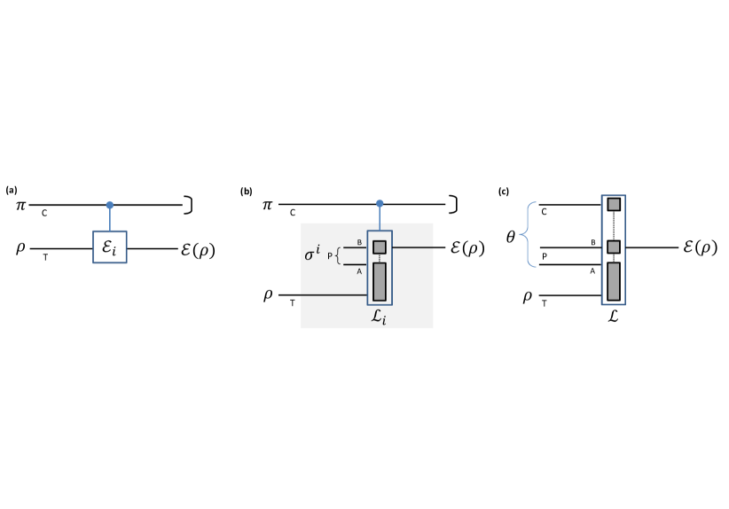
Figure 1: Steps for conditional channel simulation, as described in Sec. II of the main text. In panels (b) and (c), we also depict the LOCC structure of the trace-preserving quantum operations $\mathcal{L}_{i}$ and $\mathcal{L}$.

II.2 Conditional channel simulation

Consider the classical state

$$\pi_{C}:={\textstyle\sum\nolimits_{i}}p_{i}\left|i\right\rangle_{C}\left\langle i\right|,$$ (5)

where $\left|i\right\rangle$ is the computational orthonormal basis of a control qudit $C$ whose dimension is equal to the number $N$ of elements in the ensemble $\{\mathcal{E}_{i}\}$. Let us introduce the quantum operator

$$M:={\textstyle\sum\nolimits_{i}}\mathcal{C}_{i}\otimes\mathcal{E}_{i},$$ (6)

where

$$\mathcal{C}_{i}(\pi)=|{i}\rangle_{C}\langle i|\pi|{i}\rangle_{C}\langle i|.$$ (7)

As depicted in Fig. 1(a), we may then write

$$\mathcal{E}(\rho_{T}) =\mathrm{Tr}_{C}\left[M(\pi_{C}\otimes\rho_{T})\right]$$ (8)

$$=\mathrm{Tr}_{C}\left[{\textstyle\sum\nolimits_{i}}p_{i}\left|i\right\rangle_{C}\left\langle i\right|\otimes\mathcal{E}_{i}(\rho_{T})\right].$$ (9)

Note that the conditional channel expression in Eq. (9) has been also studied in the setting of degradable channels in order to show single-letter convex decompositions of the unassisted quantum capacity Smith .

Now, let us replace $\mathcal{E}_{i}$ with its simulation of Eq. (3) as also shown in Fig. 1(b),

$$M(\rho_{CT})=\sum_{i}\mathcal{C}_{i}^{C\rightarrow C}\otimes\mathcal{L}_{i}^{PT\rightarrow T}(\sigma_{P}^{i}\otimes\rho_{CT})~{}.$$ (10)

As a result, inserting the above equation into Eq. (8), we may write

$$\mathcal{E}(\rho_{T}) =\mathrm{Tr}_{C}\left[{\textstyle\sum\nolimits_{i}}p_{i}\left|i\right\rangle_{C}\left\langle i\right|\otimes\mathcal{L}_{i}^{PT\rightarrow T}(\sigma_{P}^{i}\otimes\rho_{T})\right]$$ (11)

$$=\mathcal{L}_{CPT\rightarrow T}(\theta_{CP}\otimes\rho_{T}),$$ (12)

where we introduce the “control-program” state

$$\theta_{CP}:={\textstyle\sum\nolimits_{i}}p_{i}\left|i\right\rangle_{C}\left\langle i\right|\otimes\sigma_{P}^{i},$$ (13)

and the “control-program-target” LOCC

$$\mathcal{L}_{CPT\rightarrow T}(\rho):=\mathrm{Tr}_{C}\left[{\textstyle\sum\nolimits_{i}}\mathcal{C}_{i}^{C\rightarrow C}\otimes\mathcal{L}_{i}^{PT\rightarrow T}(\rho)\right],$$ (14)

which is local with respect to systems $C$, $B$, and $AT$. The final representation of Eq. (12) is also shown in Fig. 1(c).

II.3 Stretching and single-letter bounds

We may use the channel simulation of Eq. (12) to stretch an adaptive protocol of private communication over the average channel $\mathcal{E}={\textstyle\sum\nolimits_{i}}p_{i}\mathcal{E}_{i}$. Assuming that Alice and Bob have local registers $\mathbf{a}$ and $\mathbf{b}$, and that they perform adaptive LOCCs between each channel transmission, we may apply the teleportation stretching procedure of Ref. PLOB , where each channel use is replaced with its LOCC simulation (12). Considering $n$ uses of the channel, we may write Alice and Bob’s output state as

$$\rho_{\mathbf{ab}}^{n}=\Lambda(\theta_{CP}^{\otimes n}),$$ (15)

where $\Lambda$ is a trace-preserving LOCC including the adaptive LOCCs of the protocol and the simulation LOCCs, while $\theta_{CP}$ is the control-program state of Eq. (13).

Using results from Ref. PLOB , we may bound the key rate achievable by any adaptive protocol of key generation over $\mathcal{E}$. Consider an $\varepsilon$-secure protocol with output $\rho_{\mathbf{ab}}^{n}$ where $\left\|\rho_{\mathbf{ab}}^{n}-\phi_{n}\right\|<\varepsilon$ and $\phi_{n}$ is a private state with $nR_{n}$ secret bits. Then, the $n$-use key rate $R_{n}^{\varepsilon}$ must satisfy

$$R_{n}^{\varepsilon}\leq\frac{E_{R}(\rho_{\mathbf{ab}}^{n})+2H_{2}(\varepsilon)}{(1-4\varepsilon\alpha)n},$$ (16)

where $\alpha$ is a constant parameter associated to the dimension $d$ of the private state $\phi_{n}$ and $H_{2}(\varepsilon)=-\varepsilon\log_{2}\varepsilon-(1-\varepsilon)\log_{2}(1-\varepsilon)$ is the binary Shannon entropy. In particular, we may always choose $\alpha$ such that $\mathrm{log}_{2}d\leq\alpha nR_{n}^{\varepsilon}$ for both discrete- and continuous-variable systems Chr ; TQC ; PLOB . For the specific case of entanglement distribution (so that the target state is not a private state but a maximally entangled state of $nR_{n}^{\varepsilon}$ ebits), we can simply set $\alpha=1$.

The previous bound is simplified by using Eq. (15) and basic properties of the REE. In fact, we may write

$$E_{R}(\rho_{\mathbf{ab}}^{n})\overset{(1)}{\leq}E_{R}(\theta_{CP}^{\otimes n})$$ (17)

$$\overset{(2)}{\leq}nE_{R}(\theta_{CP})$$ (18)

$$\overset{(3)}{=}nE_{R}\left({\textstyle\sum\nolimits_{i}}p_{i}\left|i\right\rangle_{C}\left\langle i\right|\otimes\sigma_{P}^{i}\right)$$ (19)

$$\overset{(4)}{\leq}n{\textstyle\sum\nolimits_{i}}p_{i}E_{R}(\left|i\right\rangle_{C}\left\langle i\right|\otimes\sigma_{P}^{i})$$ (20)

$$\overset{(5)}{\leq}n{\textstyle\sum\nolimits_{i}}p_{i}E_{R}(\sigma_{P}^{i}),$$ (21)

where we have used: (1) the monotonicity of the REE under trace-preserving LOCCs as $\Lambda$; (2) the subadditivity of the REE over tensor products; (3) the definition of control-program state $\theta_{CP}$; (4) the convexity of the REE over mixtures of states Donald ; and (5) the subadditivity of the REE over the tensor product $\left|i\right\rangle_{C}\left\langle i\right|\otimes\sigma_{P}^{i}$ where we may always assume that the separable state $\left|i\right\rangle_{C}\left\langle i\right|$ belongs to Alice. More precisely, let us set $P=AB$ and denote by $\sigma_{CA|B}^{\text{sep}}$ a state which is separable with respect to the split $CA|B$. Then, in terms of the relative entropy $S(.||.)$, we may write

$$E_{R}(\left|i\right\rangle_{C}\left\langle i\right|\otimes\sigma_{AB}^{i})$$ (22)

$$=\inf_{\sigma_{CA|B}^{\text{sep}}}S(\left|i\right\rangle_{C}\left\langle i\right|\otimes\sigma_{AB}^{i}~{}||~{}\sigma_{CA|B}^{\text{sep}})$$ (23)

$$\leq\inf_{\sigma_{A|B}^{\text{sep}}}S(\left|i\right\rangle_{C}\left\langle i\right|\otimes\sigma_{AB}^{i}~{}||~{}\left|i\right\rangle_{C}\left\langle i\right|\otimes\sigma_{A|B}^{\text{sep}})$$ (24)

$$=\inf_{\sigma_{A|B}^{\text{sep}}}S(\sigma_{P}^{i}~{}||~{}\sigma_{A|B}^{\text{sep}}):=E_{R}(\sigma_{AB}^{i}).$$ (25)

By replacing Eq. (18) in Eq. (16), we therefore derive

$$R_{n}^{\varepsilon}\leq\frac{E_{R}(\theta_{CP})}{1-4\varepsilon\alpha}+\frac{2H_{2}(\varepsilon)}{(1-4\varepsilon\alpha)n}.$$ (26)

Now, by taking the limit for large $n$ and small $\varepsilon$ (weak converse), and also using Eq. (21), we may write

$$\lim_{n,\varepsilon}R_{n}^{\varepsilon}\leq E_{R}(\theta_{CP})\leq{\textstyle\sum\nolimits_{i}}p_{i}E_{R}(\sigma_{P}^{i}).$$ (27)

Finally, by taking the supremum over all adaptive key generation protocols $\mathcal{P}$, we get the secret key capacity of the channel

$$K(\mathcal{E})=\sup_{\mathcal{P}}\lim_{n,\varepsilon}R_{n}^{\varepsilon}\leq E_{R}(\theta_{CP})\leq{\textstyle\sum\nolimits_{i}}p_{i}E_{R}(\sigma_{P}^{i}),$$ (28)

where the last inequality is expressed in terms of the REE of the program states $\sigma_{P}^{i}$ of the channel components $\mathcal{E}_{i}$. Recall that, for an arbitrary channel $\mathcal{E}$, we may write the chain of (in)equalities

$$D_{2}(\mathcal{E})=Q_{2}(\mathcal{E})\leq P_{2}(\mathcal{E})=K(\mathcal{E}),$$ (29)

where $D_{2}$ is the two-way assisted entanglement distribution capacity, $Q_{2}$ is the two-way assisted quantum capacity, and $P_{2}$ is the two-way assisted private capacity. Therefore, Eq. (28) provides upper bounds for all the capacities in Eq. (29).

Remark 1

While the first inequality in Eq. (28) never appeared in the literature to our knowledge, the final inequality $K(\mathcal{E})\leq{\textstyle\sum\nolimits_{i}}p_{i}E_{R}(\sigma_{P}^{i})$ in Eq. (28) can also be obtained from a probabilistic argument where a channel component $\mathcal{E}_{i}$ with probability $p_{i}$ appears $np_{i}$ times in an asymptotic protocol with large $n$. Therefore, this component provides $np_{i}$ copies of the program state $\sigma_{i}$ in the stretching of the adaptive protocol. Overall, one has the output state $\Lambda(\otimes_{i}\sigma_{i}^{np_{i}})$ PLOB leading to the same final inequality as in Eq. (28).

Remark 2

Because the conditional channel simulation is independent from probabilistic/asymptotic arguments, we may write the result directly for finite $n$. In particular, we have that Eq. (26) directly leads to the following finite-size upper bound

$$R_{n}^{\varepsilon}\leq\frac{{\textstyle\sum\nolimits_{i}}p_{i}E_{R}(\sigma_{P}^{i})}{1-4\varepsilon\alpha}+\frac{2H_{2}(\varepsilon)}{(1-4\varepsilon\alpha)n}.$$ (30)

for any $(n,\varepsilon,R_{n}^{\varepsilon})$-adaptive protocol implemented over an average channel $\mathcal{E}=\textstyle\sum\nolimits_{i}p_{i}\mathcal{E}_{i}$ with program states $\sigma_{P}^{i}$.

III Applications in finite dimension

III.1 Diagonal amplitude damping channel

Here we apply the result to a diagonal type of amplitude damping channel (DAD) that may be represented as

$$\mathcal{E}_{p}^{\text{DAD}}=p\mathcal{E}_{0}+(1-p)\mathcal{E}_{1},$$ (31)

where $\mathcal{E}_{0}(\rho):=\mathrm{Tr}(\rho)\left|0\right\rangle\left\langle 0\right|$ and $\mathcal{E}_{1}=\mathcal{I}$ is the identity channel (note that this channel coincides with the standard amplitude damping channel only when it is applied to the computational basis). The channel $\mathcal{E}_{0}$ is teleportation covariant and entanglement-breaking, so that it allows for a LOCC simulation with a separable program state and, accordingly, $E_{R}=0$. At the same time, $\mathcal{E}_{1}=\mathcal{I}$ is teleportation covariant with $E_{R}(\rho_{\mathcal{I}})=1$. Therefore, from Eq. (28), it is easy to compute

$$K(\mathcal{E}_{p}^{\text{DAD}})\leq 1-p.$$ (32)

Note that $\mathcal{E}_{0}$ are $\mathcal{E}_{1}$ are not jointly teleportation covariant. In fact, given a Pauli operator $P\in\{I,X,Y,Z\}$, this is exactly commuted by the identity, but different is the case for $\mathcal{E}_{0}$ for which we have

$$\mathcal{E}_{0}(Z\rho Z^{\dagger})=Z\mathcal{E}_{0}(\rho)Z^{\dagger},~{}~{}\mathcal{E}_{0}(X\rho X^{\dagger})=\mathcal{E}_{0}(\rho).$$ (33)

Since the output unitaries become different for the two channel components, these are not jointly teleportation covariant and the DAD channel is not teleportation covariant. For this reason, we cannot write $K(\mathcal{E}_{p}^{\text{DAD}})\leq E_{R}(\rho_{\mathcal{E}_{p}^{\text{DAD}}})$. Nonetheless, since each $\mathcal{E}_{i}$ in Eq. (31) is individually teleportation covariant, we can use the conditional channel simulation that allows us to write the upper bound of Eq. (28) in terms of the Choi matrices of the components. The very simple form of the REE bound in Eq. (32) has the advantage to make it easily extendable to repeater chains and quantum networks net .

III.2 Erasure pipeline

Consider an arbitrary qubit channel $\mathcal{N}$ which is followed by an erasure channel $\mathcal{E}_{p}^{\text{erase}}$ mapping the input state into an orthogonal erasure state $|e\rangle$ with probability $p$. Explicitly we may write the erasure pipeline $\mathcal{E}_{p}^{\text{pipe}}:=\mathcal{E}_{p}^{\text{erase}}\circ\mathcal{N}$ as follows

$$\mathcal{E}_{p}^{\text{pipe}} =(1-p)\mathcal{N}+p\mathcal{E}_{e},$$ (34)

$$\mathcal{E}_{e}(\rho) :=\mathrm{Tr}(\rho)|e\rangle\langle e|~{}.$$ (35)

Assume that $\mathcal{N}$ can be LOCC-simulated with a program state $\sigma_{\mathcal{N}}$. We may write a conditional channel simulation for $\mathcal{E}_{p}^{\text{pipe}}$ and then use Eq. (28) to derive the upper bound

$$K(\mathcal{E}_{p}^{\text{pipe}})\leq(1-p)E_{R}(\sigma_{\mathcal{N}}).$$ (36)

Here we use the fact that the channel $\mathcal{E}_{e}$ is teleportation covariant and entanglement-breaking ($E_{R}=0$). It is clear that Eq. (36) also applies to a pipeline of a $d$-dimensional qudit channel $\mathcal{N}_{d}$ followed by a $d$-dimensional erasure channel [whose output is therefore $(d+1)$-dimensional].

III.3 Dephrasure channel

As an example of erasure pipeline, consider the “dephrasure channel” Dephra , which is a dephasing channel $\mathcal{E}_{q}^{\text{deph}}$ with dephasing probability $q$, followed by an erasure channel $\mathcal{E}_{p}^{\text{erase}}$. Explicitly we may write the dephrasure channel $\mathcal{E}_{p,q}^{\text{dr}}:=\mathcal{E}_{p}^{\text{erase}}\circ\mathcal{E}_{q}^{\text{deph}}$ as follows

$$\mathcal{E}_{p,q}^{\text{dr}}(\rho)=(1-p)\left[(1-q)\rho+qZ\rho Z\right]+p\mathcal{E}_{e}(\rho),$$ (37)

where $Z$ is the phase-flip Pauli operator. Note that the channel components $\mathcal{E}_{q}^{\text{deph}}$ and $\mathcal{E}_{e}$ are teleportation-covariant but not jointly. Using Eq. (36) with the fact that the dephasing channel is simulable with its Choi matrix $\rho_{\mathcal{E}_{q}^{\text{deph}}}$, we derive

$$K(\mathcal{E}_{p}^{\text{pipe}})\leq(1-p)E_{R}\left(\rho_{\mathcal{E}_{q}^{\text{deph}}}\right)=(1-p)[1-H_{2}(q)],$$ (38)

where $H_{2}$ is the usual binary Shannon entropy.

Now we prove that the previous relation holds with an equality. In fact, assume that, at the output of the channel, we use a dichotomic measurement with operators $\left|e\right\rangle\left\langle e\right|$ and $I-\left|e\right\rangle\left\langle e\right|$. This measurement fully decodes the second (erasure) channel $\mathcal{E}_{p}^{\text{erase}}$, i.e., with probability $1-p$ we post-select the first (dephasing) channel $\mathcal{E}_{q}^{\text{deph}}$. It is then known that the two-way entanglement distribution capacity $D_{2}$ of $\mathcal{E}_{q}^{\text{deph}}$ is equal to $1-H_{2}(q)$ PLOB . As a result, an asymptotically achievable rate for entanglement distribution over a dephrasure channel is equal to

$$D_{2}(\mathcal{E}_{p,q}^{\text{dr}})\geq(1-p)[1-H_{2}(q)].$$ (39)

From Eqs. (38) and (39) we therefore conclude the exact formulas

$$Q_{2}(\mathcal{E}_{p,q}^{\text{dr}}) =D_{2}(\mathcal{E}_{p,q}^{\text{dr}})=P_{2}(\mathcal{E}_{p,q}^{\text{dr}})$$ (40)

$$=K(\mathcal{E}_{p,q}^{\text{dr}})=(1-p)[1-H_{2}(q)].$$ (41)

Note that we cannot achieve the lower bound in Eq. (39) using the reverse coherent information (RCI) of the channel RCI . In fact, let us write the Kraus decomposition of the dephrasure channel, which is

$$\mathcal{E}_{p,q}^{\text{dr}}(\rho)=\sum_{k=0}^{3}E_{k}\rho E_{k}^{\dagger},$$ (42)

with operators

$$E_{0} =\sqrt{(1-p)(1-q)}(|0\rangle\langle 0|+|1\rangle\langle 1|)~{},$$ (43)

$$E_{1} =\sqrt{(1-p)q}(|0\rangle\langle 0|-|1\rangle\langle 1|)~{},$$ (44)

$$E_{2} =\sqrt{p}|e\rangle\langle 0|,~{}E_{3}=\sqrt{p}|e\rangle\langle 1|~{}.$$ (45)

We then find its Choi matrix

$$\rho_{\mathcal{E}_{p,q}^{\text{dr}}} =\frac{1-p}{2}|\Phi\rangle\langle\Phi|+\frac{p}{2}(|0e\rangle\langle 0e|+|1e\rangle\langle 1e|)$$ (46)

$$-q(|00\rangle\langle 11|+|11\rangle\langle 00|),$$ (47)

where $|\Phi\rangle=(|00\rangle+|11\rangle)/\sqrt{2}$. As a result, we compute the RCI of the dephrasure channel to be

$$I_{\text{RC}}(\mathcal{E}_{p,q}^{\text{dr}})=(1-p)[1-H_{2}(q)]-H_{2}(p)~{}.$$ (48)

This expression correctly reduces to $1-p-H_{2}(p)$ when $q=0$, which is the RCI of the erasure channel PLOB . Because $\mathcal{E}_{p,q}^{\text{dr}}$ is not unital, we have that its RCI is different from its coherent information, which is given by Dephra

$$I_{\text{C}}(\mathcal{E}_{p,q}^{\text{dr}})=(1-p)[1-H_{2}(q)]-p~{}.$$ (49)

IV Extension to continuous variables

IV.1 Asymptotic simulations

The conditional channel simulation can be extended to ensembles of channels having asymptotic simulations, such as bosonic channels or the amplitude damping channel PLOB . This means that we may consider an average channel $\mathcal{E}=\sum_{i}p_{i}\mathcal{E}_{i}$ where each channel component $\mathcal{E}_{i}$ may have a generally-asymptotic LOCC simulation as PLOB

$$\mathcal{E}_{i}(\rho_{T})=\lim_{\mu}\mathcal{L}_{i,\mu}^{PT\rightarrow T}(\sigma_{P}^{i,\mu}\otimes\rho_{T}),$$ (50)

where $\mathcal{L}_{i,\mu}^{PT\rightarrow T}$ is a sequence of LOCCs (between Alice and Bob) and $\sigma_{P}^{i,\mu}$ is a sequence of program states. Eq. (50) means that the distance between channel $\mathcal{E}_{i}$ and its asymptotic simulation, as measured by the energy-constrained diamond norm TQC ; PLOB , goes to zero in the asymptotic limit. For instance, $\mathcal{E}_{i}$ may be a teleportation-covariant bosonic channel, so that we may choose a sequence of Choi-approximating program states

$$\sigma_{P}^{i,\mu}=\rho_{\mathcal{E}_{i}}^{\mu}:=\mathcal{I}\otimes\mathcal{E}_{i}(\Phi^{\mu}),$$ (51)

where $\Phi^{\mu}$ is a two-mode squeezed vacuum (TMSV) state with variance $\mu$ RMP . Perfect simulation is then obtained in the limit $\mu\rightarrow\infty$.

In general, we may therefore write the following simulation for the average channel

$$\mathcal{E}(\rho_{T})=\lim_{\mu}\mathcal{L}_{CPT\rightarrow T}^{\mu}(\theta_{CP}^{\mu}\otimes\rho_{T}),$$ (52)

where we consider a sequence of control-program states

$$\theta_{CP}^{\mu}:=\sum_{i}p_{i}~{}\left|i\right\rangle_{C}\left\langle i\right|\otimes\sigma_{P}^{i,\mu},$$ (53)

based on orthogonal states $\left|i\right\rangle$, and a sequence of LOCCs

$$\mathcal{L}_{CPT\rightarrow T}^{\mu}(\rho):=\mathrm{Tr}_{C}\left[\sum_{i}\mathcal{C}_{i}^{C\rightarrow C}\otimes\mathcal{L}_{i,\mu}^{PT\rightarrow T}(\rho)\right],$$ (54)

where $\mathcal{C}_{i}$ is defined in Eq. (7).

These equations are a full extension of previous Eqs. (12), (13) and (14). Correspondingly, we may extend the stretching of Eq. (15) and write

$$\rho_{\mathbf{ab}}^{n}=\lim_{\mu}\Lambda_{\mu}(\theta_{CP}^{\mu\otimes n}),$$ (55)

for a sequence of LOCCs $\Lambda_{\mu}$ NotaBOUND . Then, repeating the reasonings of Sec. II.3 and using arguments from Ref. PLOB , we may write

$$E_{R}(\rho_{\mathbf{ab}}^{n}) =\inf_{\sigma_{\text{sep}}^{(n)}}S(\rho_{\mathbf{ab}}^{n}||\sigma_{\text{sep}}^{(n)})$$ (56)

$$\overset{(1)}{\leq}\inf_{\sigma_{\text{sep}}^{\mu}}S\left[\lim_{\mu}\Lambda_{\mu}(\theta_{CP}^{\mu\otimes n})~{}||~{}\lim_{\mu}\sigma_{\text{sep}}^{\mu\otimes n}\right]$$ (57)

$$\overset{(2)}{\leq}\inf_{\sigma_{\text{sep}}^{\mu}}\underset{\mu}{\text{{liminf}}}~{}S\left[\Lambda_{\mu}(\theta_{CP}^{\mu\otimes n})~{}||~{}\sigma_{\text{sep}}^{\mu\otimes n}\right]$$ (58)

$$\overset{(3)}{\leq}\inf_{\sigma_{\text{sep}}^{\mu}}\underset{\mu}{\text{{liminf}}}~{}S\left[\Lambda_{\mu}(\theta_{CP}^{\mu\otimes n})~{}||~{}\Lambda_{\mu}(\sigma_{\text{sep}}^{\mu\otimes n})\right]$$ (59)

$$\overset{(4)}{\leq}\inf_{\sigma_{\text{sep}}^{\mu}}\underset{\mu}{\text{{liminf}}}~{}S\left(\theta_{CP}^{\mu\otimes n}~{}||~{}\sigma_{\text{sep}}^{\mu\otimes n}\right)$$ (60)

$$\overset{(5)}{=}n\inf_{\sigma_{\text{sep}}^{\mu}}\underset{\mu}{\text{{liminf}}}~{}S\left(\theta_{CP}^{\mu}~{}||~{}\sigma_{\text{sep}}^{\mu}\right)$$ (61)

$$\overset{(6)}{\leq}n\sum_{i}p_{i}~{}\inf_{\sigma_{\text{sep}}^{i,\mu}}\underset{\mu}{\text{{liminf~{}}}}S\left(\sigma_{P}^{i,\mu}~{}||~{}\sigma_{\text{sep}}^{i,\mu}\right)$$ (62)

$$\overset{(7)}{=}n\sum_{i}p_{i}~{}E_{R}(\sigma_{P}^{i})$$ (63)

where: (1)$~{}\sigma_{\text{sep}}^{\mu}$ is a sequence of separable states such that $\|\sigma_{\text{sep}}-\sigma_{\text{sep}}^{\mu}\|\overset{\mu}{\rightarrow}0$ for separable $\sigma_{\text{sep}}$, and $\sigma_{\text{sep}}^{(n)}=\sigma_{\text{sep}}^{\otimes n}$ is a suboptimal choice; (2) we use the lower semi-continuity of the relative entropy $S$ HolevoBOOK ; (3) we use that $\Lambda_{\mu}(\sigma_{\text{sep}}^{\mu\otimes n})$ are specific types of separable sequences; (4) we use the monotonicity of $S$ under $\Lambda_{\mu}$; (5) we use the additivity of $S$ over tensor products; (6) we use the definition of $\theta_{CP}^{\mu}$ given in Eq. (53) and the joint convexity of $S$ which can be applied by replacing $\sigma_{\text{sep}}^{\mu}$ with $\sum_{i}p_{i}~{}\sigma_{\text{sep}}^{i,\mu}$ [the orthogonal states $\left|i\right\rangle_{C}\left\langle i\right|$ can be discarded using the same arguments of Eqs. (22)-(25)]; and (7) we define the REE of an asymptotic state $\sigma:=\lim_{\mu}\sigma^{\mu}$ as follows PLOB

$$E_{R}(\sigma):=\inf_{\sigma_{\text{sep}}^{\mu}}\underset{\mu}{\text{{liminf}}}S\left(\sigma^{\mu}~{}||~{}\sigma_{\text{sep}}^{\mu}\right),$$ (64)

with $\|\sigma_{\text{sep}}-\sigma_{\text{sep}}^{\mu}\|\overset{\mu}{\rightarrow}0$ for separable $\sigma_{\text{sep}}$.

Using the weaker asymptotic definition of REE of Eq. (64), we may therefore write the upper bound

$$K(\mathcal{E})\leq\sum_{i}p_{i}~{}E_{R}(\sigma_{P}^{i}).$$ (65)

For computing this upper bound we need to calculate the REE of the program states $\sigma_{P}^{i,\mu}=\sigma_{AB}^{i,\mu}$ by considering a split between Alice ($A$) and Bob ($B$). Typically, one computes a further upper bound which comes from picking a candidate separable state in the minimization of the REE, i.e.,

$$E_{R}(\sigma_{P}^{i}) :=\inf_{\sigma_{\text{sep}}^{p,\mu}}\underset{\mu}{\text{{liminf}}}S\left(\sigma_{P}^{i,\mu}~{}||~{}\sigma_{\text{sep}}^{i,\mu}\right)$$ (66)

$$\leq\underset{\mu}{\text{{liminf}}}S(\sigma_{P}^{i,\mu}~{}||~{}\tilde{\sigma}_{\text{sep}}^{i,\mu}).$$ (67)

If $\sigma_{P}^{i,\mu}$ and $\tilde{\sigma}_{\text{sep}}^{i,\mu}$ are Gaussian states, then we can use a closed formula for their relative entropy, given in Ref. PLOB . Contrary to previous formulations, the formula for the relative entropy between two arbitrary multimode Gaussian states established in Ref. PLOB is directly expressed in terms of their statistical moments, without the need of symplectic diagonalizations (for more details see Theorem 6 and Remark 7 of Ref. TQC ).

IV.2 Continuous ensembles

Besides asymptotic simulations, we can also extend the tool to continuous ensembles with associated probability densities. This means that we may consider an average channel defined by

$$\mathcal{E}=\int di~{}p_{i}~{}\mathcal{E}_{i}~{},$$ (68)

where each channel component $\mathcal{E}_{i}$ may have a generally-asymptotic LOCC simulation PLOB , i.e., of the form in Eq. (50). We may extend all the previous formulas with the replacement

$${\textstyle\sum\nolimits_{i}}p_{i}~{}\rightarrow\int di~{}p_{i}~{}.$$ (69)

In particular, we may write the simulation of Eq. (52) but with a sequence of control-program states

$$\theta_{CP}^{\mu}:=\int di~{}p_{i}~{}\left|i\right\rangle_{C}\left\langle i\right|\otimes\sigma_{P}^{i,\mu},$$ (70)

where $\left|i\right\rangle$ are orthogonal states, and a sequence of LOCCs

$$\mathcal{L}_{CPT\rightarrow T}^{\mu}(\rho):=\mathrm{Tr}_{C}\left[\int di~{}\mathcal{C}_{i}^{C\rightarrow C}\otimes\mathcal{L}_{i,\mu}^{PT\rightarrow T}(\rho)\right].$$ (71)

This leads again to the stretching of Eq. (55) and then to the following upper bound

$$K(\mathcal{E})\leq\int di~{}p_{i}~{}E_{R}(\sigma_{P}^{i}),$$ (72)

where $\sigma_{P}^{i}:=\lim_{\mu}\sigma_{P}^{i,\mu}$ and $E_{R}(\sigma_{P}^{i})$ has the asymptotic expressions in Eqs. (66) and (67).

V Applications to non-Gaussian mixtures

V.1 Ensembles of lossy channels

Let us consider the non-Gaussian average channel $\mathcal{E}:=\sum_{i}p_{i}\mathcal{E}_{i}$, where $\mathcal{E}_{i}:=\mathcal{E}_{\eta_{i}}$ is a lossy channel with transmissivity $\eta_{i}$ and associated probability $p_{i}$. The asymptotic Choi matrix of the average channel $\rho_{\mathcal{E}}=\lim_{\mu}\rho_{\mathcal{E}}^{\mu}$ is defined over the sequence $\rho_{\mathcal{E}}^{\mu}=\mathcal{I}\otimes\mathcal{E}(\Phi^{\mu})$ with $\Phi^{\mu}$ being a TMSV state. Also note that we may write

$$\rho_{\mathcal{E}}^{\mu}=\sum_{i}p_{i}\rho_{\mathcal{E}_{i}}^{\mu},$$ (73)

where $\rho_{\mathcal{E}_{i}}^{\mu}$ are the quasi-Choi matrices of the single channel components $\mathcal{E}_{i}:=\mathcal{E}_{\eta_{i}}$. Each channel component $\mathcal{E}_{i}$ is teleportation covariant and therefore simulable by teleporting the input over its asymptotic Choi matrix PLOB . More precisely, one has the asymptotic simulation in Eq. (50) where $\mathcal{L}_{i,\mu}^{PT\rightarrow T}$ is a generalized Braunstein-Kimble protocol teleCV and $\sigma_{P}^{i,\mu}=\rho_{\mathcal{E}_{i}}^{\mu}$.

Note that the LOCC $\mathcal{L}_{i,\mu}^{PT\rightarrow T}$ depends on the loss parameter $\eta_{i}$ which means that the channel components $\mathcal{E}_{i}$ are not jointly teleportation-covariant. For this reason, the simulation of the non-Gaussian mixture $\mathcal{E}$ is not via its asymptotic Choi matrix but can be written in the conditional and asymptotic form of Eq. (52) with $\sigma_{P}^{i,\mu}=\rho_{\mathcal{E}_{i}}^{\mu}$. Using Eqs. (65) and (67), we compute the upper bound

$$K(\mathcal{E})\leq{\textstyle\sum\nolimits_{i}}p_{i}\underset{\mu}{~{}\text{{liminf}}}~{}S(\rho_{\mathcal{E}_{i}}^{\mu}||\tilde{\sigma}_{\text{sep}}^{i,\mu}),$$ (74)

for a suitable separable Gaussian state $\tilde{\sigma}_{\text{sep}}^{i,\mu}$. From Ref. PLOB , we know that the inferior limit provides the PLOB bound $-\log_{2}(1-\eta_{i})$. Therefore, one has

$$K(\mathcal{E})\leq-{\textstyle\sum\nolimits_{i}}p_{i}\log_{2}(1-\eta_{i}).$$ (75)

Let us now derive a lower bound by computing the RCI of the average channel $\mathcal{E}$ in terms of the sequence $\rho_{\mathcal{E}}^{\mu}$

$$I_{RC}(\mathcal{E}) =\lim_{\mu}I(A\langle B)_{\rho_{\mathcal{E}}^{\mu}},$$ (76)

$$I(A\langle B)_{\rho_{\mathcal{E}}^{\mu}} =S(\rho_{A}^{\mu})-S(\rho_{\mathcal{E}}^{\mu}),$$ (77)

where $S(.)$ is the von Neumann entropy and we have set $\rho_{A}^{\mu}=\mathrm{Tr}_{B}\rho_{\mathcal{E}}^{\mu}$. Note that for any $\rho=\sum_{i}p_{i}\rho_{i}$ we may use the concavity properties NC00

$${\textstyle\sum\nolimits_{i}}p_{i}S(\rho_{i})\leq S\left(\rho\right)\leq{\textstyle\sum\nolimits_{i}}p_{i}S(\rho_{i})+H(\{p_{i}\}),$$ (78)

where $H(\{p_{i}\}):=-\sum_{i}p_{i}\log p_{i}$ is the Shannon entropy. Therefore, from Eq. (73), we may write

$$I(A\langle B)_{\rho_{\mathcal{E}}^{\mu}}=S(\mathrm{Tr}_{B}\rho_{\mathcal{E}}^{\mu})-S(\rho_{\mathcal{E}}^{\mu})$$ (79)

$$=S\left({\textstyle\sum\nolimits_{i}}p_{i}\mathrm{Tr}_{B}\rho_{\mathcal{E}_{i}}^{\mu}\right)-S\left({\textstyle\sum\nolimits_{i}}p_{i}\rho_{\mathcal{E}_{i}}^{\mu}\right)$$ (80)

$$\geq{\textstyle\sum\nolimits_{i}}p_{i}S(\mathrm{Tr}_{B}\rho_{\mathcal{E}_{i}}^{\mu})-{\textstyle\sum\nolimits_{i}}p_{i}S(\rho_{\mathcal{E}_{i}}^{\mu})-H(\{p_{i}\})$$ (81)

$$={\textstyle\sum\nolimits_{i}}p_{i}I(A\langle B)_{\rho_{\mathcal{E}_{i}}^{\mu}}-H(\{p_{i}\}).$$ (82)

Therefore, from Eq. (76) we get

$$I_{RC}(\mathcal{E})=\lim_{\mu}{\textstyle\sum\nolimits_{i}}p_{i}I(A\langle B)_{\rho_{\mathcal{E}_{i}}^{\mu}}-H(\{p_{i}\})$$ (83)

$$={\textstyle\sum\nolimits_{i}}p_{i}I_{RC}(\mathcal{E}_{i})-H(\{p_{i}\})$$ (84)

$$=-{\textstyle\sum\nolimits_{i}}p_{i}\log_{2}(1-\eta_{i})-H(\{p_{i}\}),$$ (85)

where we have used the fact that the RCI of the lossy channel $\mathcal{E}_{i}:=\mathcal{E}_{\eta_{i}}$ is simply $I_{RC}(\mathcal{E}_{i})=-\log_{2}(1-\eta_{i})$ PLOB . As a result, we may write the sandwich

$$-{\textstyle\sum\nolimits_{i}}p_{i}\log_{2}(1-\eta_{i})-H(\{p_{i}\})\leq Q_{2}(\mathcal{E})$$ (86)

$$\leq K(\mathcal{E})\leq-{\textstyle\sum\nolimits_{i}}p_{i}\log_{2}(1-\eta_{i}).$$ (87)

V.2 Continuous ensembles of lossy channels

Note that we may also consider a continuous ensemble of lossy channels with different transmissivities, i.e., the non-Gaussian channel

$$\mathcal{E}:=\int d\eta~{}p_{\eta}\mathcal{E}_{\eta},$$ (88)

for some suitable probability density $p_{\eta}$. It is easy to repeat previous steps and write the upper bound

$$K(\mathcal{E})\leq-\int d\eta~{}p_{\eta}\log_{2}(1-\eta).$$ (89)

Another continuous ensemble of lossy channels can be created by considering a beam splitter operation between the system and the environment

$$\mathcal{\tilde{E}}_{\eta}(\rho):=\mathrm{Tr}_{E}[U_{\eta}^{\text{BS}}(\rho\otimes\sigma_{E})U_{\eta}^{\text{BS}\dagger}]~{},$$ (90)

where in the above definition $\eta$ is the transmissivity and $\sigma_{E}$ is a reference state of the environment. For the bosonic lossy channel $\sigma_{E}$ is the vacuum state, while in the thermal-loss channel $\sigma_{E}$ is a thermal state. In general, one can write any Gaussian and non-Gaussian state using the Glauber $P$-representation

$$\sigma_{E}=\int d^{2}\gamma~{}p_{\gamma}\left|\gamma\right\rangle\left\langle\gamma\right|\,,$$ (91)

where $\left|\gamma\right\rangle$ is a coherent state with amplitude $\gamma$. If the state $\sigma_{E}$ is classical, then $p_{\gamma}$ is a classical probability density, and we can easily show that the non-Gaussian channel $\mathcal{\tilde{E}}_{\eta}(\rho)$ is represented by the average

$$\mathcal{\tilde{E}}_{\eta}(\rho)=\int d^{2}\gamma~{}p_{\gamma}\,\mathcal{E}_{\eta,\gamma}(\rho)~{},$$ (92)

where $\mathcal{E}_{\eta,\gamma}$ is a displaced lossy channel

$$\mathcal{E}_{\eta,\gamma}(\rho) =\mathrm{Tr}_{E}[U_{\eta}^{\text{BS}}(\rho\otimes\left|\gamma\right\rangle_{E}\left\langle\gamma\right|)U_{\eta}^{\text{BS}\dagger}]$$ (93)

$$=D(\gamma\sqrt{1-\eta})\,\mathcal{E}_{\eta,0}(\rho)\,D^{\dagger}(\gamma\sqrt{1-\eta}),$$ (94)

with $D(\alpha)=\exp(\alpha a^{\dagger}-\alpha^{\ast}a)$ being the displacement operator RMP in terms of the ladder operators $a$ and $a^{\dagger}$.

Let us write the beam-splitter action

$$U_{\eta}^{\text{BS}}a^{\dagger}U_{\eta}^{\text{BS}\dagger}=\cos\theta a^{\dagger}-\sin\theta a_{E}^{\dagger},$$ (95)

where $\cos^{2}\theta=\eta$ and $a^{\dagger}$ ($a_{E}^{\dagger}$) is the creation operator acting on the system (environment). We may show that the non-Gaussian channel $\mathcal{\tilde{E}}_{\eta}$ is teleportation covariant. In fact, we have

$$\mathcal{E}_{\eta,\gamma}[D(z)\,\rho\,D(-z)]=D(z\cos\theta)\,\mathcal{E}_{\eta,\gamma}\left(\rho\right)\,D(-z\cos\theta).$$ (96)

Since the correction unitary $D(z\cos\theta)$ does not depend on $\gamma$, we have that the channels $\mathcal{E}_{\eta,\gamma}$ are jointly teleportation covariant with respect to $\gamma$. As a result, $\mathcal{\tilde{E}}_{\eta}$ is teleportation covariant and simulable with its asymptotic Choi matrix $\rho_{\mathcal{\tilde{E}}_{\eta}}=\lim_{\mu}\rho_{\mathcal{\tilde{E}}_{\eta}}^{\mu}$ where $\rho_{\mathcal{\tilde{E}}_{\eta}}^{\mu}=\mathcal{I}\otimes\mathcal{\tilde{E}}_{\eta}(\Phi^{\mu})$. Therefore, we may write the upper bound

$$K(\mathcal{\tilde{E}}_{\eta})\leq\underset{\mu}{\text{{liminf}}}S(\rho_{\mathcal{\tilde{E}}_{\eta}}^{\mu}||\tilde{\sigma}_{\text{sep}}^{\eta,\mu}),$$ (97)

for some suitable separable state $\tilde{\sigma}_{\text{sep}}^{\eta,\mu}$. Note that the quasi-Choi matrix takes the form

$$\rho_{\mathcal{\tilde{E}}_{\eta}}^{\mu}=\int d^{2}\gamma~{}p_{\gamma}\,\rho_{\mathcal{E}_{\eta,\gamma}}^{\mu}$$ (98)

$$=\int d^{2}\gamma~{}p_{\gamma}~{}[I\otimes D(\gamma\sin\theta)]\,\rho_{\mathcal{E}_{\eta,0}}^{\mu}[I\otimes D(-\gamma\sin\theta)].$$ (99)

Since the relative entropy does not depend on displacements, we may write

$$K(\mathcal{\tilde{E}}_{\eta})\leq\underset{\mu}{\text{{liminf}}}S(\rho_{\mathcal{E}_{\eta,0}}^{\mu}||\tilde{\sigma}_{\text{sep}}^{\eta,\mu})=-\log(1-\eta),$$ (100)

so that the PLOB bound applies to the non-Gaussian channel $\mathcal{\tilde{E}}_{\eta}$ for any classical state $\sigma_{E}$ of the environment.

VI Extension to memory channels

The conditional channel simulation can also be used to represent memory quantum channels. Let us consider $M$ channel ensembles simultaneously acting on $M$ quantum systems, i.e.,

$$\mathcal{E}_{\mathbf{i}}=\mathcal{E}_{i_{1}}^{1}\otimes\mathcal{E}_{i_{2}}^{2}\otimes\cdots\otimes\mathcal{E}_{i_{M}}^{M},$$ (101)

where the instance $\mathbf{i}=i_{1},i_{2},\cdots,i_{M}$ occurs with joint probability $p_{\mathbf{i}}$. The process is memoryless if and only if the probability is factorized as $p_{\mathbf{i}}=p_{i_{1}}p_{i_{2}}\cdots p_{i_{M}}$, otherwise there is a classical memory among the channels.

Consider the average $M$-system channel

$$\mathcal{E}={\textstyle\sum\nolimits_{\mathbf{i}}}p_{\mathbf{i}}\mathcal{E}_{\mathbf{i}}~{}.$$ (102)

In order to write its conditional simulation, we extend the formulas of Sec. II.2 by means of the replacement $i\rightarrow\mathbf{i}$. Therefore, we may write Eq. (8) where

$$\pi_{C}:={\textstyle\sum\nolimits_{\mathbf{i}}}p_{\mathbf{i}}\left|\mathbf{i}\right\rangle_{C}\left\langle\mathbf{i}\right|,~{}~{}M:={\textstyle\sum\nolimits_{\mathbf{i}}}\left|\mathbf{i}\right\rangle_{C}\left\langle\mathbf{i}\right|\otimes\mathcal{E}_{\mathbf{i}},$$ (103)

with $\left|\mathbf{i}\right\rangle=\left|i_{1}\right\rangle\left|i_{2}\right\rangle\otimes\cdots\otimes\left|i_{M}\right\rangle$ being the computational orthonormal basis of a control system $C$. Let us replace $\mathcal{E}_{i_{k}}^{k}$ by its simulation with program state $\sigma_{P}^{k,i_{k}}$. Then, we may write Eq. (12) with the “control-program” state

$$\theta_{CP}:={\textstyle\sum\nolimits_{\mathbf{i}}}p_{\mathbf{i}}\left|\mathbf{i}\right\rangle_{C}\left\langle\mathbf{i}\right|\otimes{\textstyle\bigotimes\nolimits_{k=1}^{M}}\sigma_{P}^{k,i_{k}}.$$ (104)

Assuming an adaptive protocol over $n$ uses of $\mathcal{E}$, we may write the stretching of the output state $\rho_{\mathbf{ab}}^{n}$ as in Eq. (15) and derive

$$K(\mathcal{E}) \leq{\textstyle\sum\nolimits_{\mathbf{i}}}p_{\mathbf{i}}E_{R}\left({\textstyle\bigotimes\nolimits_{k=1}^{M}}\sigma_{P}^{k,i_{k}}\right)$$ (105)

$$\leq{\textstyle\sum\nolimits_{\mathbf{i}}}p_{\mathbf{i}}{\textstyle\sum\nolimits_{k=1}^{M}}E_{R}\left(\sigma_{P}^{k,i_{k}}\right),$$ (106)

with suitable extensions to asymptotic simulations and continuous ensembles.

VII Conclusions

In this work we have designed a tool for channel simulation which is particularly helpful for mixtures of channels. This simulation is based on the use of a control system which generates the probability distribution associated with the channel ensemble; the state of this control system is then included in the final program state. In this way we can handle mixtures of teleportation-covariant channels which are not jointly covariant, and we can simulate non-Gaussian channels and memory channels.

The conditional channel simulation can be exploited in the stretching of adaptive protocols, so that we may bound the two-way quantum and private capacities in terms of the REE. This allowed us to establish all the two-way capacities of the recently introduced “dephrasure” channel. We have also derived bounds for various non-Gaussian channels that can be described in terms of ensembles of lossy channels.

Note that these bounds can also be derived by using the probabilistic arguments of Ref. PLOB . However, the tool of conditional channel simulation not only allows us to derive these asymptotic results without probabilistic arguments but also allows one to consider finite-size versions which are valid for any finite number of uses.

Acknowledgments. This work have been supported by the EPSRC via the ‘UK Quantum Communications Hub’ (EP/M013472/1) and by the European Union via Continuous Variable Quantum Communications (CiViQ, Project ID: 820466). LB has been supported by the EPSRC grant EP/K034480/1.

References

• (1) J. Watrous, The theory of quantum information (Cambridge University Press, Cambridge, 2018).
• (2) M. Hayashi, Quantum Information Theory: Mathematical Foundation (Springer-Verlag Berlin Heidelberg, 2017).
• (3) C. H. Bennett, D. P. DiVincenzo, J. A. Smolin, and W. K. Wootters, Phys. Rev. A 54, 3824-3851 (1996).
• (4) C. H. Bennett, G. Brassard, C. Crepeau, R. Jozsa, A. Peres, and W. K. Wootters, Phys. Rev. Lett. 70, 1895 (1993).
• (5) S. Pirandola et al., Nat. Photon. 9, 641-652 (2015).
• (6) G. Bowen and S. Bose, Phys. Rev. Lett. 87, 267901 (2001).
• (7) S. Pirandola, R. Laurenza, C. Ottaviani, and L. Banchi, Nat. Commun. 8, 15043 (2017).
• (8) C. Weedbrook et al., Rev. Mod. Phys. 84, 621 (2012).
• (9) S. Pirandola, S. L. Braunstein, R. Laurenza, C. Ottaviani, T. P. W. Cope, G. Spedalieri, and L. Banchi, Quantum Sci. Technol. 3, 035009 (2018).
• (10) M. A. Nielsen and I. L. Chuang, Phys. Rev. Lett. 79, 321 (1997).
• (11) S. Ishizaka, and T. Hiroshima, Phys. Rev. Lett. 101, 240501 (2008).
• (12) S. Ishizaka, and T. Hiroshima, Phys. Rev. A 79, 042306 (2009).
• (13) S. Ishizaka, Some remarks on port-based teleportation, arXiv:1506.01555 (2015).
• (14) M. Studzinski, S. Strelchuk, M.Mozrzymas and M. Horodecki, Sci. Rep. 7, 10871 (2017).
• (15) S. Pirandola, R. Laurenza, and C. Lupo, Fundamental limits to quantum channel discrimination, arXiv:1803.02834 (2018).
• (16) V. Vedral, Rev. Mod. Phys. 74, 197 (2002).
• (17) V. Vedral, M. B. Plenio, M. A. Rippin, and P. L. Knight, Phys. Rev. Lett. 78, 2275-2279 (1997).
• (18) V. Vedral, and M. B. Plenio, Phys. Rev. A 57, 1619 (1998).
• (19) F. Leditzky, D. Leung, and G. Smith, Dephrasure channel and superadditivity of the coherent information, arXiv: 1806.08327v1 (2018).
• (20) G. Smith, and J. A. Smolin, Proceedings of the IEEE Information Theory Workshop 2008. pp 368-372.
• (21) N. Hosseinidehaj, and R. Malaney, Phys. Rev. A 91, 022304 (2015).
• (22) Recall that the Choi matrix of a quantum channel $\mathcal{E}$ is defined by propagating part of a maximally entangled state through the channel. For a qubit channel, we therefore have $\rho_{\mathcal{E}}:=\mathcal{I}\otimes\mathcal{E}(\Phi)$ where $\mathcal{I}$ is the identity channel and $\Phi:=\left|\Phi\right\rangle\left\langle\Phi\right|$, with $\left|\Phi\right\rangle$ being a Bell state.
• (23) Recall that a quantum channel $\mathcal{E}_{i}$ is teleportation covariant if, for any teleportation unitary $U$ (unitary matrix from the Weyl-Heisenberg group), there exists some unitary $V_{i}$ such that PLOB $\mathcal{E}_{i}(U\rho U^{\dagger})=V_{i}\mathcal{E}_{i}(\rho)V_{i}^{\dagger}$.
• (24) M. Christiandl, A. Ekert, M. Horodecki, P. Horodecki, J. Oppenheim, and R. Renner, Lecture Notes in Computer Science 4392, 456-478 (2007). See also quant-ph/0608199v3 (2006).
• (25) M. J. Donald, and M. Horodecki, Phys. Lett. A 264, 257-260 (1999).
• (26) S. Pirandola, Capacities of repeater-assisted quantum communications, arXiv:1601.00966 (2016).
• (27) Recall that the RCI $I_{\text{RC}}(\mathcal{E})$ of a quantum channel $\mathcal{E}$ is defined as the reverse coherent information when the input state is a maximally entangled state, so that it is computed over the channel’s Choi matrix PLOB .
• (28) S. L. Braunstein and H. J. Kimble, Phys. Rev. Lett. 80, 869–872 (1998).
• (29) M. A. Nielsen and I. L. Chuang, Quantum Computation and Quantum Information (Cambridge University Press, Cambridge, 2000).
• (30) More precisely the limit in Eq. (55) can be written in trace norm if we suitably bound the energy of Alice’s and Bob’s registers, a condition which can be assumed in the background of the calculations and then relaxed at the very end. See Ref. TQC  for technical details.
• (31) A. Holevo, Quantum Systems, Channels, Information: A Mathematical Introduction (De Gruyter, Berlin-Boston, 2012).