A High-Performance Interactive Computing Framework for Engineering Applications

Abstract

To harness the potential of advanced computing technologies, efficient (real time) analysis of large amounts of data is as essential as are front-line simulations. In order to optimise this process, experts need to be supported by appropriate tools that allow to interactively guide both the computation and data exploration of the underlying simulation code. The main challenge is to seamlessly feed the user requirements back into the simulation. State-of-the-art attempts to achieve this, have resulted in the insertion of so-called check- and break-points at fixed places in the code. Depending on the size of the problem, this can still compromise the benefits of such an attempt, thus, preventing the experience of real interactive computing. To leverage the concept for a broader scope of applications, it is essential that a user receives an immediate response from the simulation to his or her changes. Our generic integration framework, targeted to the needs of the computational engineering domain, supports distributed computations as well as on-the-fly visualisation in order to reduce latency and enable a high degree of interactivity with only minor code modifications. Namely, the regular course of the simulation coupled to our framework is interrupted in small, cyclic intervals followed by a check for updates. When new data is received, the simulation restarts automatically with the updated settings (boundary conditions, simulation parameters, etc.). To obtain rapid, albeit approximate feedback from the simulation in case of perpetual user interaction, a multi-hierarchical approach is advantageous. Within several different engineering test cases, we will demonstrate the flexibility and the effectiveness of our approach.

1 Introduction

Simulation of very complex physical phenomena becomes a realistic endeavour with the latest advances in hardware technologies, sophisticated (numerical) algorithms, and efficient parallelisation strategies. It consists of modelling a domain of a physical problem, applying appropriate boundary conditions, and doing numerical approximation for the governing equations, often with a linear or non-linear system as outcome. When the system is solved, the result is validated and visualised for more intuitive interpretations.

All the aforementioned cycles – pre-processing, computation, and post-processing – can be very time consuming, depending on the discretisation parameters, e. g., and moreover, are traditionally carried out as a sequence of steps. The ever-increasing range of specialists in developing engineering fields has necessitated an interactive approach with the computational model. This requires real-time feedback from the simulation during program runtime, while experimenting with different simulation setups. For example, the geometry of the simulated scene can be modified interactively altogether with boundary conditions or a distinct feature of the application, thus, the user can gain “insight concerning parameters, algorithmic behaviour, and optimisation potentials” Mulder.1999 .

Interactive computing frameworks, libraries, and Problem Solving Environments (PSEs) are used by specialists to interact with complex models, while not requiring deep knowledge in algorithms, numerics, or visualisation techniques. These are user-friendly facilities for guiding the numerically approximated problem solution. The commonly agreed features are: a sophisticated user interface for the visualisation of results on demand and a separated steerable, often time- and memory-consuming simulation running on a high-performance computer (see Fig. 1).

A user guides an often time and memory consuming simulation in order to build a solution to his/her problem via a graphical user interface.

The concept has been present in the scientific and engineering community already for more than two decades. Meanwhile, numerous powerful tools serving this purpose have been developed. A brief overview of some state-of-the-art tools – steering environments and systems such as CSE vanLiere.1996 , Magellan Vetter.1997 , SCIRun Parker.1998 , Uintah deStGermain.2000 , G-HLAM Rycerz.2006 and EPSN Nicolas.2007 , libraries such as CUMULVS Geist.1997 , or RealityGrid Brooke.2003 ; Pickles.2004 , or frameworks such as Steereo Jenz.2010 – is provided in the next section. Those tools differ in the way they provide interactive access to the underlying simulation codes, using check- and breakpoints, satellites connected to a data manager, or data flow concepts, e. g., hence they cannot always fully exploit interactive computing and are usually of limited scope concerning different application domains.

2 Computational Steering – State of the art

CSE vanLiere.1996 is a computational steering environment consisting of a very simple, flexible, minimalistic kernel and modular components, so-called satellites, where all the higher level functionality is pushed. It is based on the idea of a central process, i. e. a data manager to which all the satellites can be connected. Satellites can create and read/write variables, and they can subscribe to events such as notification of mutations of a particular variable Mulder.1995 . The data manager informs all the satellites of changes made in the data and an interactive graphics editing tool allows users to bind data variables to user interface elements.

CUMULVS Geist.1997 is a library that provides steering functionality so that a programmer can extract data from a running (possibly parallel) simulation and send those data to the visualisation package. It encloses the connection and data protocols needed to attach multiple visualisation and steering components to a running application during execution. The user has to declare in the application which parameters are allowed to be modified or steered, or the rules for the decomposition of the parallel data, etc. Using check-pointing, the simulation can be restarted according to the new settings.

In the steering system called Magellan Vetter.1997 , steering objects are exported from an application. A collection of instrumentation points, such as so-called actuators, know how to change an object without disrupting application execution. Pending update requests are stored in a shared buffer until an application thread polls for them  Vetter.1997 .

EPSN Nicolas.2007 API is a distributed computational steering environment, where an XML description of simulation scripts is introduced to handle data and concurrency at instrumentation points. There is a simple connection between the steering servers, i. e. simulation back ends, and clients, i. e. user interfaces. When receiving requests, the server determines their date, thus, the request is executed as soon as it fulfills a condition. Reacting on a request means releasing the defined blocking points.

Steereo Jenz.2010 is a light-weight steering framework, where the client can send requests and the simulation will respond to them. However, the requests are not processed immediately, but rather stored in a queue and executed at predefined points in the simulation code. Hence, users have to define when and how often this queue should be processed.

The RealityGrid Brooke.2003 ; Pickles.2004 project has provided a highly flexible and robust computing infrastructure for supporting the modelling of complex systems RealityGrid.2003 . An application is structured into a client, a simulation, and a visualisation unit communicating via calls to the steering library functions. Also this infrastructure involves the insertion of check- and break-points at fixed places in the code where changed parameters are obtained and the simulation is to be restarted.

In the SCIRun Parker.1998 problem solving environment (PSE) for modelling, simulation, and visualisation of scientific problems, a user may smoothly construct a network of required modules via a visual programming interface. Computer simulations can then be executed, controlled, and tuned interactively, triggering the re-execution only of the necessary modules, due to the underlying dataflow model. It allows for extension to provide real-time feedback even for large scale, long-running, data-intensive problems. This PSE has typically been adopted to support pure thread-based parallel simulations so far. Uintah deStGermain.2000 is a component-based visual PSE that builds upon the best features of the SCIRun PSE, specifically addressing the massively parallel computations on petascale computing platforms.

In the G-HLAM Rycerz.2006 PSE, the focus is more on fault tolerance, i. e. monitoring and migration of the distributed federates. The group of main G-HLAM services consists of one which coordinates management of the simulation, one which decides when performance of a federate is not satisfactory and migration is required, the other which stores information about the location of local services. It uses distributed federations on the Grid for the communication among simulation and visualisation components.

All of those powerful tools have, however, either limited scope of application, or are involving major simulation code changes in order to be effective. This was the motivation for us to design a new framework that incorporates the strong aspects of the aforementioned tools, nevertheless overcomes their weak aspects in order to provide a generic concept for a plenitude of different applications with minimal codes changes and a maximum of interactivity.

Within the Chair for Computation in Engineering at Technische Universität München, a series of successful Computational Steering research projects took place in the previous decade. It has also involved collaboration with industry partners. Performance analysis has been done for several interactive applications, in regard to responsiveness to steering, and the factors limiting performance have been identified. The focus at this time was on interactive computational fluid dynamics (CFD), based on the Lattice-Boltzmann method, including a Heating Ventilation Air-Conditioning (HVAC) system simulator Borrmann.2005 , online-CFD simulation of turbulent indoor flows in CAD-generated virtual rooms Wenisch.2004 , interactive thermal comfort assessment vanTreeck.2007 , and also on structure mechanics – computational methods in orthopaedics. Over time, valuable observations and experience have resulted in significant reduction of the work required to extend an existing application code for steering.

Again, the developed concepts have been primarily adapted to this limited number of application scenarios, thus, they allow for further investigations so as to become more efficient, generic, and easy to implement. This is where our framework comes into play.

3 The Idea of the Framework

For widening the scope of the steerable applications, an immediate response of any simulation back end to the changes made by the user is required. Hence, the regular course of the simulation has to be interrupted as soon as a user interacts. Within our framework, we achieve this using the software equivalent of hardware interrupts, i. e. signals. The check for updates is consequently done in small, user-defined, cyclic intervals, i. e., within a function handling the Unix ALARM signal.

If the check does not indicate any update from the user side, the simulation gets the control back and continues from the state saved at the previous interrupt-point. Otherwise, the new data is received, matched to the simulation data (which is the responsibility of the user himself), and simulation state variables (for instance loop delimiters) are manipulated in order to make the computation stop and then automatically start anew according to the user modifications. Taking the pseudo code of an iteratively executed function (within several nested loops) as an example, the redundant computation is skipped as soon as the end of the current, most-inner loop iteration is reached. This is, namely, the earliest opportunity to compare the values of the simulation state variables, and, if the result of the comparison indicates so, exit all the loops (i. e. starting with most-inner one and finishing with the most-outer one) Knezevic.2011a ; Knezevic.2011b ; Knezevic.2010 . This would exactly mean starting computation over again, as illustrated in the pseudocode:

% X_end, Y_end declared global

begin function Signal_Handler()
  % manipulate X_end, Y_end so that the redundant
  % computation is skipped and started anew
  X_end = Y_end = -1
end

% set time interval for periodically occurence of
% ALARM signal to stop execution and call handler
Set_Alarm()

% user function to be interrupted
begin function Compute()
  for t = T_start to T_end do
    for i = X_start to X_end do
      for j = Y_start to Y_end do
        Process(data[i][j])
        % potential update is recognised next
      od
    od
  od
end

As elaborated in Knezevic.2010 , to guarantee the correct execution of a program, one should use certain type qualifiers (provided by ANSI C, e. g.) for the variables which are subject to sudden change or objects to interrupts. One should ensure that certain types of objects which are being modified both in the signal handler and the main computation are updated in an atomic way. Furthermore, if the value in the signal handler has changed, the outdated value in the register should not be used again. Instead, the new value should be loaded from memory. This may occur due to the custom compiler optimisations. In addition to this, sufficient steps have to be taken to prevent potentially introduced severe memory leaks before the new computation is started. This is due to the interrupts and their possible occurrence before the memory allocated at a certain point has been released.

Finally, with either one or several number of iterations being finished without an interrupt, new results are handed on to the user process for visualisation. One more time it is the user’s responsibility to prescribe to the front end process how to interpret the received data so that it can be coherently visualised Knezevic.2011a ; Knezevic.2011b ; Knezevic.2010 ; Knezevic.2011c ; Knezevic.2011d .

In Fortran, similar to C/C++, support for signal handling can be enabled at user level with minimal efforts involved. Some vendor supplied Fortran implementations, including for example Digital, IBM, Sun, and Intel, have the extension that allows the user to do signal handling as in C Baloai.2008 . Here, a C wrapper function for overriding the default signal behaviour has to be implemented. However, the behaviour of the Fortran extension of the aforementioned function is implementation dependent, and if the application is compiled using an Intel Fortran compiler, when the program is interrupted, it will terminate unless one “clears” the previously defined action first.

Due to the accuracy requirements and the increasing amount of data which has to be handled in numerical simulations of complex physical phenomena nowadays, there is an urge to fully exploit the general availability and increasing CPU power of high-performance computers. For this, in addition to efficient algorithms and data structures, sophisticated parallel programming methods are a constraint. The design of our framework, therefore, takes into consideration and supports different parallel paradigms, which results in an extra effort to ensure correct program execution and avoid synchronisation problems when using threads, as explained in the following subsection.

3.1 Multithreading Parallelisation Scenario

We consider the scenario when pure multithreading (with, e. g., OpenMP/POSIX threads) is employed in the computations on the simulation side. Since a random thread is interrupted via signal at the expiration of the user-specified interval, that thread probes, via the functionality of the Message Passing Interface (MPI), if any information regarding the user activity is available. If the aforesaid checking for a user’s message indicates that an update has been sent, the receiving thread instantly obtains all the information and applies necessary manipulations in order to re-start the computation with the changed setting. Hence, all other threads also become instantly aware that their computations should be started over again and must now proceed in a way in which clean termination of the parallel region is guaranteed.

3.2 “Hybrid” Parallelisation Scenario

In a “hybrid” parallel scenario (i. e. MPI and OpenMP – see Fig. 3.2), a random thread in each active process is being interrupted, hence, fetches an opportunity to check for the updates. The rest of the procedure is similar as described for the pure multithreading, except that now all the processes have to be explicitly notified about the changes performed by a user. This may involve additional communication overheads. Moreover, if one master process, which is the direct interface of the user’s process to the computing-nodes, i. e. slaves, is supposed to inform all of them about the user updates, it may become a bottleneck. Therefore, a hierarchical non-blocking broadcast algorithm for transferring the signal to all computing nodes has been proposed in Knezevic.2011a ; Knezevic.2011b .

In the case of a hybrid parallel scenario, each process is doing its own checks for updates; one random thread per process is interrupted in small, fixed time intervals.

4 Applications

In the following, a few application scenarios are presented, where the implemented framework has been successfully integrated. First, a simple 2D simulation of a temperature conduction, used only for testing purposes, where heat sources, boundaries of the domain, etc. can be interactively modified. Then, a neutron transport simulation developed at the Nuclear Engineering Program, University of Utah, which has been the first Fortran test case for the framework. The next one is the sophisticated Problem Solving Environment SCIRun developed at the Scientific Computing and Imaging (SCI) Institute, University of Utah. The final one is a tool for pre-operative planning of hip-joint surgeries, done as a collaborative project of the Chair for Computation in Engineering and Computer Graphics and Visualization at Technische Universität München. A summary of necessary modifications of the original codes in order to integrate the framework is discussed in section 5.2.

4.1 Test Case 1 – A Simple Heat Conduction Simulation

Simulation: For proof of concept, we consider as a first, very simple example a 2D simulation of heat conduction in a given region over time. It is described by the Laplace equation, whose solutions are characterised by a gradual smoothing of the starting temperature distribution by the heat flow from warmer to colder areas of a domain. Thus, different states and initial conditions will tend toward a stable equilibrium. After numerical treatment of the PDE via a Finite Difference scheme, we come up with a five-point stencil. The Gauss-Seidel iteration method is used to solve the resulting linear system of equations.

GUI/Visualisation: For interacting with the running simulation, a graphical user interface is provided using the wxWidgets library wxWidgets . The variations of the height along the z-axes, pointing upward, are representing the variations of the temperature in the corresponding 2D domain. Both the simulation and the visualisation are implemented in C++ and are separate MPI processes.

User interaction: When it comes to the interplay with the program during the simulation, there are a few possibilities available – one can interactively add, delete, or move heat sources, add, delete, or move boundary points of the domain, or change the termination condition (maximal number of iterations or error tolerance) of the solver. As soon as a user interacts, the simulation becomes immediately aware of it and consequently the computation is restarted. An instant estimation of the equilibrium state for points of the domain far away from the heat sources is unfortunately not always feasible on the finest grid used (300$\times$300). This may be the case due to the short intervals between two restarts in case of too frequent user interaction, as shown in Fig. 1. Here we profit from a hierarchical approach.

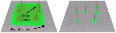
Figure 1: Left: an initial scenario; right: moving heat sources/boundaries leads to the restart of the computation, but in-between two too frequent restarts a user is unable to estimate the equilibrium temperature in the region farther away from the heat sources (here, further iterations of the solver would be necessary).

The hierarchical approach is based on switching between several grids of different resolutions depending on the frequency of the user interaction. At the beginning, the finest desired grid is used for the computation. When the simulation process is interrupted by an update, it restarts the computation with the new settings, but on a coarser grid for faster feedback, i. e. to provide new results as soon as possible. As long as the user is frequently interacting, all computations are carried out on the coarser grids only. If the user halts, i. e. stops interacting, the computation switches back to the finest grid in order to provide more accurate values. In this particular test case, three different grids were used – an initial 300$\times$300 grid, the four times smaller, intermediate one (150$\times$150, in case of lower pace of interactions, i. e. adding/deleting heat sources or boundary points, e. g.) and, finally, the coarsest one (75$\times$75) for very high frequency moving of boundary points or heat sources over the domain (Fig. 2). The coarser grids are not meant for obtaining quantitative solutions, just for a fast qualitative idea how the solution might look like. If a user interactively found an interesting setup, he just has to stop and an accurate solution for this setup will be computed. Nevertheless, measurements concerning the different grids showed that the variation of the solution on the finest grid compared to the intermediate one is around 4.5%, and compared to the coarsest one around 14.6%. The described approach, on the other hand, leads to an improvement in convergence by a factor of 2.

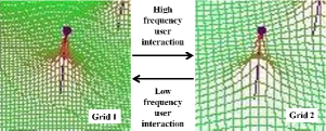
Figure 2: Switching to a coarser grid in case of moving heat sources or boundaries, switching back to the finer one once the user stops interacting.

Additionally, we employ a multi-level algorithm – the results of the computation on the coarsest grid are not discarded when switching to the finer one. Our concept, namely, already involves a hierarchy of discretisations, as is the case in multigrid algorithms, thus, we can profit from the analogous idea. Our scheme is somewhat simpler – it only starts with the solution on the coarsest grid and uses the result we gain as an initial guess of the result on a finer one. A set of examples has been tested (with grids 300$\times$300, 150$\times$150, and 75$\times$75) where the number of necessary operations on the intermediate and fine grid could be halved. What seems to be a somehow obvious approach, at least for this simple test scenario, can be efficiently exploited in our forth test case where we use hierarchical Ansatz functions for an interactive finite-element computation of a biomedical problem.

In order to enable the framework functionality for interrupting the above simulation, takes an experienced user a couple of hours at most. Implementing the hierarchical approach (which is not a part of the framework) is more time consuming (a few working days), since an optimal automatic detection when to switch from one hierarchy to another has to be found—which requires numerous experiments.

4.2 Test Case 2 – A Neutron Transport Simulation

We present as second test case the integration of the framework into a computationally efficient, high accuracy, geometry independent neutron transport simulation. It makes researchers’ and educators’ interaction with virtual models of nuclear reactors or their parts possible.

Simulation: AGENT (Arbitrary GEometry Neutron Transport) solves the Boltzmann transport equation, both in 2D and 3D, using the Method of Characteristics (MOC) Lee.2004 . The motivation for steering such a simulation during runtime comes mostly from the geometric limitation of this method, which requires fine spatial discretisation in order to provide an accurate solution to the problem. On the other hand, a good initial solution guess would help tremendously to speed-up the convergence, and this property is used to profit from our framework. The 3D discretisation basis for the Boltzmann equation consists of the discrete number of plains, for each of which both a regular geometry mesh and a number of parallel rays in a discrete number of directions are generated. The approximation results in a system of equations to be iteratively solved for discrete fluxes.

GUI/Visualisation: The result in terms of the scalar fluxes is simultaneously calculated and periodically visualised. The simulation server maintains a list of available simulation states, and clients connect using the ImageVis3D volume rendering tool Fogal.2010 to visualise the results in real time. Users can interfere with the running simulation via a simple console interface, providing the new values of the desired parameters.

User interaction: Instant response of the simulation to the changes made by the user is again achieved via signals. Using the technique described as our general concept, the most outer iteration instantly starts anew, as soon as its overall state is reset within the main computational steering loop, according to the updated settings and necessary re-initialisation of the data. By manipulating only two simulation parameters in the signal handler, it is achieved that the iteration restarts almost within a second in all the cases – e. g. 20 planes in z-direction, each discretised by a 300$\times$300 grid and 36 azimuthal angles (where only one, the most outer iteration lasts approximately 500 seconds). The effort to integrate our framework into this application depends on whether the re-allocation of the memory and re-initialisation of the data is required, and if one wants to re-use the values from the previous iterations Knezevic.2012a ; Knezevic.2012b .

Hierarchical and multilevel approach: It is likely, similar to the heat conduction scenario, that the user wants to accelerate the convergence by starting calculations with lower accuracy (i. e. number of azimuthal angles, see Fig. 3), preserve and re-use some of the values from the previous calculation as an initial guess for the higher accuracy solution. For a conceptually similar algorithm, such as the previously described multilevel approach in the 2D heat conduction simulation, we have seen that our framework has given promising results. The re-initialisation of the data for this, most challenging, scenario is a part of imminent research.

Figure 3: Experimenting with different numbers of azimuthal angles, small values are given to simplify the picture.

To briefly conclude on this application scenario, the integration of the framework has been straightforward and also not very time consuming. After examining the initial code, deciding which variables to register within the framework, and writing reinitialisation routines, it has taken a few hours to couple the components together and enable visualisation after each iteration. The major effort refers actually to the re-initialisation of variables at the beginning of each “new” computation, i. e. after a user interaction, which is also not a responsibility of the framework itself.

4.3 Test Case 3 – Extension of a Problem Solving Environment

Simulation: As mentioned before, SCIRun is a PSE intended for interactive construction, debugging, and steering of large-scale, typically parallel, scientific computations Shepherd.2009 . SCIRun simulations are designed as networks of computational components, i. e. modules connected via input/output ports. This makes it very easy for a programmer to modify a module without affecting others. As SCIRun is already a mature, sophisticated environment for computational steering, nevertheless, our goal is to improve it in a way that real time feedback for extensive time- and memory-consuming simulations becomes possible. Here, SCIRun needs to finish an update first before new results are shown, which easily can lead to long latencies between cause and effect.

GUI/Visualisation: For the user, it is possible to view intermediate results after a pre-defined number of iterations, while the calculations continue to progress. At some point, he may require to influence the current simulation setup. Different options such as parameter modification for each module are available via corresponding interfaces. Both the modified module and modules whose input data is dependent on that module’s output are stored in a queue for execution. Our intention is to interrupt the module currently being executed and skip the redundant cycles, as well as to remove any module previously scheduled for execution from the actual queue.

User Interaction: The concept has been tested on several examples to evaluate the simulation response to the modifications during runtime. These scenarios are: a simulation that facilitates early detection of acute heart ischemia and two defibrillation-like simulations – one on a homogeneous cube and the other on a human torso domain. The challenges of getting an immediate feedback/response of the simulation depend on a few factors – the size of the problem, the choice of the modified parameters within the simulation, etc. The earlier in the execution pipeline the parameter appears, the more modules have to be re-executed, thus, the more challenging it is to provide the real-time response to the user changes. A user can define different discretisation parameters for a FEM computation such as the mesh resolution for all spatial directions. For solving the resulting linear system of equations, different iterative solvers as well as pre-conditioners can be used; one may change tolerances, the maximal number of iterations, levels of accuracy, as well as other numerical or some more simulation-specific parameters. In the created network of modules, typically the most laborious step is the SolveLinearSystem module. Thus, the first challenge is how to interrupt it as soon as any change is made by the user – in particular, the changes done via UI to this module. To achieve this in the algorithm of the linear equation solver, the maximal number of iterations (a user interface variable) is manipulated in the signal handler, so as to be set to some value outside of the domain of the iterator index which interrupts the simulation as described before. The execute function of this module also has to be re-scheduled afterward with the new user-applied settings. However, one has to take care that the previous interrupted execution of the same module is finished in a clean way and that the execute function has to be called anew (in order to trigger re-computation instantly). If one chooses to emit the partial solution after each iteration, executions of several visualisation modules are scheduled after each iteration, which would take additional few seconds after each iteration. This is because after an interrupted iteration the preview of old results has to be cancelled. The execution of all modules, which would happen after SolveLinearSystem, has to be aborted. The scheduler cancels the execution of all the scheduled modules that have not begun yet by making sure an exception is employed. Changing any input field of a module via its UI automatically triggers the re-execution of all the modules following it in the pipeline.

Tool for early detection of heart ischemia

Myocardial ischemia is characterised by reduced blood supply of the heart muscle, usually due to coronary artery disease. It is the most common cause of death in most Western countries, and a major cause of hospital admissions  Podrid.2005 . By early detection further complications might be prevented. The aim of this application is the generation of a quasi-static volume conductor model of an ischemic heart, based on data from actual experiments  Stinstra.2012 . The generation of models of the myocardium is based on MR images/scans of a dog heart. The known values are extracellular cardiac potentials as measured by electrodes on an isolated heart or with inserted needles. The potential difference between the intracellular and extracellular space which is being calculated is not the same for ischemic and healthy cells. A network of modules is constructed within SCIRun to simulate and then render a model of the transmembrane potential of a dog’s myocardium in experiments (Fig. 4).

Defibrillation

Defibrillation therapy consists of delivering a dose of electrical energy to the heart with a device that terminates the arrhythmia and allows normal sinus rhythm to be re-established by the body’s natural pacemaker. Implantable Cardioverter Defibrillators (ICDs) are relatively common, patient specific, implantable devices that provide an electric shock to treat fatal arrhythmias in cardiac patients  Steffen.2012 . By building a computational model of a patient’s body with ICDs and mapping conductivity values over the entire domain, we can accurately compute how activity generated in one region would be remotely measured in another region  Weinstein.2005 , which is exactly what doctors would be interested in. First, we consider a simulation of the electrical conduction on a homogeneous cube domain (Fig. 4) with two electrodes placed within. Each of the electrodes is assigned a conductivity value. The effect of changing those values is explored for both of the electrodes. The second example helps to determine optimal energy discharge and placement of the ICD in the human torso (Fig. 4). A model of the torso into which ICD geometry is interactively placed is based on patient MRI or CT data. Different solver-related parameters for the resulting system of the linear equations, conductivity values, as well as mesh resolutions for a FEM computation can be applied during runtime. This allows for previewing the solution on a coarser grid and switching to finer ones, once the user is satisfied with the current setting.

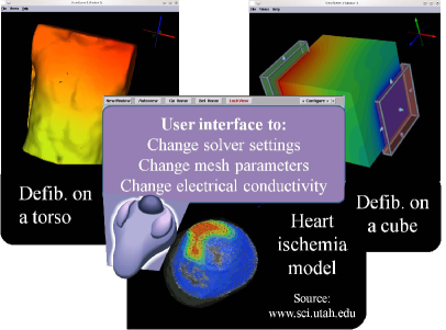
Figure 4: Illustrated user interfaces for the tested simulation scenario.

For a user to integrate the framework, the major effort has been related to re-triggering the execution of all the needed modules when the user makes a change. This has required good understanding of a used Model-View-Controller pattern. On the other hand, registering the variables which need to be manipulated within the framework to interrupt the execution of the modules of interest, has required negligible amount of time.

4.4 Test Case 4 – A Biomedical Application

Another test case is an analysis tool which assists an orthopaedic surgeon to do optimal implant selection and positioning based on prediction of response of a patient-specific bone (femur) to a load that is applied. The tool consists of two coupled components.

Simulation: The first one is a simulation core, where the generated models of femur geometry are based on CT/MRI-data and the computation is done using the Finite Cell Method (FCM). FCM is a variant of high order p-FEM, i. e. convergence is achieved by increasing the polynomial degree p of the Ansatz functions on a fixed mesh instead of decreasing the mesh sizes h as in case of classical h-FEM, with a fictitious domain approach, as proposed in Duester.2009 . With this method, models with complicated geometries or multiple material interfaces can be easily handled without an explicit 3D mesh generation. This is especially advantageous for interactive computational steering, where this typically user-interaction intensive step would have to be re-executed for each new configuration.

GUI/Visualisation The second component is a sophisticated visualisation and user interface platform that allows the intuitive exploration of the bone geometry and its mechanical response to applied loads in the physiological and the post-operative state of an implant-bone in terms of stresses and strains Dick.2008 ; Dick.2009 . Thus, after updating the settings – either after insertion/moving an implant, or testing a new position/magnitude of the forces applied to the bone – for each unknown a scalar value, i. e. the so-called von Mises stress norm, can be calculated and the overall result sent to the front end to be visualised.

Some of the challenges in developing such an analysis tool are described in more detail in Yang.2010 ; Dick.2009 ; Dick.2008 . We conveniently had the described simulation and a sophisticated user interface with visualisation module as a starting point. Due to the initial rigid communication pattern between the two components, however, a new setting could be recognised within the simulation only after the results for the previous, outdated, one have been completely calculated and sent to the user. Consequently, the higher polynomial degrees p were used, the dramatically longer became the total time until one could finally perceive the effect of his last change. The integration of our framework then comes into play not only to make the way the data is communicated more suitable for this purpose, but also to enable interrupting the simulation immediately and getting instant feedback ensued by any user interaction.

For the best performance, on the front end, the main thread (in charge of fetching user interaction data and continuous rendering), the second thread (in charge of collecting and sending updates in timely fashion, via non-blocking MPI routines), and the third thread (dedicated for waiting to receive results as soon as these are available), are not synchronised with one another. This way, we tackle the problem of long delays that would occur if one thread is responsible for everything and communication is blocked as long as the thread is busy, which would hinder the user in (smoothly) exploring the effects of his interaction.

On the simulation side, as mentioned before, a variant of FEM is used. Mainstream approaches are

• h-FEM: convergence due to smaller diameters h of elements,

• p-FEM: convergence due to higher polynomial degrees p,

• hp-FEM: combining the aformentioned ones by alternating h and p refinements,

• rp-FEM: a combination of mesh repositioning and p refinements,

• $\ldots$

In our case, for the algebraic equations gained by the p-version Finite Element Method describing the behaviour of the femur, iterative solvers such as CG or multi grid could not be efficiently deployed due to the poor condition number of the system. To make most out of the simulation performance potential, a hierarchical concept based on an octree-decomposition of the domain in combination with a nested dissection solver is used Mundani.2007 . It allows for both the design of sophisticated steerable solvers as well as for advanced parallelisation strategies, both of which are indispensable within interactive applications.

User interaction: By applying a nested dissection solver, the most time consuming step is the recursive assembly of the stiffness matrices, each corresponding to one tree node, traversing the octree bottom up. Again, cyclically-repeating signals are used for frequent checks for updates. If there is an indicator of an upcoming message from the user side, this is recognised while processing one of the tree nodes and the simulation variables are set in a way which ensures skipping the rest of them. All the recursive assembly function calls return immediately, and the new data is received in the next step of the interactive computing loop (updating one or more of the leaf nodes). Here, precious time has been saved by skipping all the redundant calculations and, thus, calculating results only for an actual setting. As soon as the whole assembly has been completed without an user interrupt, the result in terms of stresses is sent back to the front end process for visual display. However, there is an unavoidable delay of any visual feedback especially for higher p values, i. e. $p>4$, in case of the used hardware and the complexity of the geometric model. Namely, the time needed for a (full) new computation is dramatically increasing in case of increasing p. Thus, we profit from a hierarchical approach one more time. The hierarchy exploited in this approach refers to the usage of several different polynomial degrees chosen by the user (Fig. 4.4). While the user’s interplay with the simulation is very intensive, he retrieves immediate feedback concerning the effects of his changes for lower p, being able to see more accurate results (for higher p) as soon as he stops interacting and let one iteration finish. In this case, the computation is gradually switched to higher levels of hierarchy, i. e. from $p=1$ to $p=2$ to $p=4$ and so on. The number of MPI program instances, being executed in parallel for different p can be chosen by the user. A detailed communication schemes can be found in Knezevic.2011c ; Knezevic.2011d .

Direct transition from $p=6$ to $p=1$ as soon as the user changes the force’s magnitude and direction, inserts an implant or moves it, while gradually increasing from $p=1\rightarrow p=2\rightarrow p=4\rightarrow\ldots$ as soon as the user diminishes or finally stops his interaction. Hence, a qualitative feedback about stress distribution for $p=1$ or $p=2$ is received instantly, finer result for $p\geq 4$ on demand.

To get several updates per second even for higher p values, one has to employ sophisticated parallelisation strategies. Custom decomposition techniques (i. e. recursive bisection) in this scenario, as in case of long structures such as a femur, typically hinder the efficient exploitation of the underlying computing power as this leads to improper load distributions due to large separators within the nested dissection approach. Thus, our next goal has been the development of an efficient load balancing strategy for the existing structural simulation of the bone stresses.

Task scheduling strategies typically involve a trade-off between the uniform work load distribution among all processors, as well as keeping both the communication and optimisation costs minimal. For hierarchically organised tasks with bottom-up dependencies, such as in our generated octree structure, the number of processors participating in the computation decreases by a factor of eight in each level, similar to the problem posed by Minsky for the parallel summation of $2N$ numbers with $N$ processors in a binary tree Knezevic.2012c .

In interactive applications which assume the aforementioned frequent updates from user’s side, those rapid changes within the simulation and tasks’ state favour static in comparison to dynamic load balancing strategies. It would also have to be taken into consideration that certain modifications performed by a user may involve major changes of the computational model. In this case, for repeatedly achieving the optimal amount of work being assigned to each process for each new user update, the overhead-prone scheduling step has to be executed each time. Therefore, an efficient, nevertheless simple to compute scheduling optimisation approach is needed.

Since the scheduling problem can be solved by polynomial-depth backtrack search, thus, is NP complete for most of its variants, efficient heuristics have to be devised. In our case, the sizes of the tasks, as well as the dependencies among them (given by the octree structure responsible for the order of the nested dissection advance) have to be considered. By making decisions, we consider (1) the level of the task dependency in the tree hierarchy where children nodes have to be processed before their parent nodes; (2) among equal tasks (i. e. of the same dependency level) we distinguish between different levels in the tree hierarchy, calling this property the processing order. If the depth of the tree is H, tasks from level M in the tree hierarchy have the processing order of $H-M-1$. Then we form lists of priorities, based on these two criteria, since tasks inside very long branches of the tree with an estimated bigger load should be given a higher priority. Additionally, we resort to a so-called max-min order, making sure that big tasks, in terms of their estimated number of floating-point operations, are the first ones assigned to the processors. We also split a single task among several processors when mapping tasks to processors, based on the comparison of a task’s estimated work with a pre-defined ‘unit’ task. This way, arrays of tasks, so-called ‘phases’, are formed, each phase consisting of as many generated tasks as there are computing resources. Namely, taken from the priority lists, tasks are assigned to phases in round-robin manner. The results are illustrated in Fig. 5.

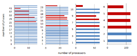
Figure 5: Vertical axes describe the so-called “phases” and the horizontal axes the number of processors involved in the particular phase. One “phase” involves actually the processors to which a task is assigned at that point. Having the capacity of each phase as full as possible is achieved, i. e. all processors are busy with the approximately equal amount of work throughout the solver execution.

Those phases refer to the mapping which will be done during runtime of the simulation. When the tasks are statically assigned to the processors, all of them execute the required computations, communicating the data when needed and also taking care that the communication delays due to the MPI internal decisions are avoided, as elaborated more in Knezevic.2012c .

Satisfactory speedup is achieved for different polynomial degrees p within the FCM computation, where higher polynomial degrees correspond to more unknowns. Tests are being done currently for a larger number of distributed memory computational resources. According to the tendency observed for up to 7 processors so far, engagement of larger numbers of processes would result in the desired rate of at least several updates per second (i. e. 1–10 Hz) for the calculated bone stresses even for $p=4$ or $p=6$.

Referring back to the existing environment, without the integration of the developed distributed parallel solver, the major effor that has been invested in creating the new communication pattern to support the described hierarchical approach was in the order of several working day. Anyhow, the functionality for interrupting the computation to do checks for updates, thus, start a computation anew if needed has been quick and straightforward.

5 Results and Conclusions

Finally, after discussing the achievements concerning interaction for each application scenario in the previous section, here results in terms of execution time overhead after integrating the framework in different scenarios are to be presented, as well as the coding effort to be invested when integrating the framework into an existing application code. Furthermore, conclusions concerning the proposed hierarchical approaches are made and possible ideas for further extension of the framework are discussed.

5.1 Overhead of the Framework

For the heat conduction application scenario, the integration of our framework resulted in not more than 5–10 % overhead in the execution time. Tests have been done also for the same problem with a message-passing-based parallel Jacobi solver. Not even in case when user interaction was invoked in 5-millisecond intervals (which is far more frequent than it typically occurs in practice) any significant effect of the interrupts on the overall execution time (less than 10 %) was to be observed.

Performance evaluation of the biomedical test scenario, where the simulation is executed on a multi-core architecture and connected to a visualisation front end via a network, still proved that the overhead caused by the framework itself is not significant (up to 11.7 %).

We have also tested the different simulation scenarios from SCIRun. The measurements have been made for different update intervals, namely, 5, 2, or 1 millisecond for different solvers of linear systems of equations. In one of the test case scenarios, for the shortest interval (i. e. 1 millisecond), the overhead caused by the framework was up to 15 %. However, by making the intervals longer (2 or 5 milliseconds, e. g.), the overhead was reduced to 5 % and 3 %, resp. When increasing the interval up to 5 milliseconds (and beyond), an end-user does not observe the difference in terms of simulation response. Hence, it is always recommendable to experiment with different intervals for a specific simulation.

Some of the measurements are illustrated in Fig. 6 for comparison.

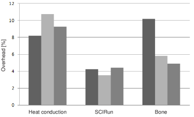
Figure 6: Performance measurements: overhead of the framework (expressed in terms of additional execution time) for alarm set to 1 millisecond – heat conduction simulation ($300\times 300$ grid), executed on 1, 2, and 4 cores (left to right); SCIRun PSE, heart ischemia example using CG, BCG, and MINRES solver (left to right); biomedical application ($p=4$), executed on 1, 2, and 4 cores (left to right).

5.2 User Effort for Integrating the Framework

A few modifications within any application code have to be made by the user in order to integrate our framework. These modifications are – as intended – only minor, hence, we list all of them. All variables which will be affected by the interrupt handler in order to force the restart of the computation have to be declared global (to become visible in a signal handler). It is typically enough to have only few of them, such as loop delimiters, in order to skip all the redundant computations. If these variables shall be used also in the rest of the code, a user can rename those he wants to manipulate within the signal handler and declare only those as global. Atomicity of data updates and prevention of compiler optimisations – which would lead to incorrect value references – have to be ensured. The integrity of each user-defined ‘atomic’ sequence of instructions in the simulation code has to be provided. The calls to the appropriate send and receive functions which are interface to our framework have to be included in the appropriate places in the code. The user himself should provide the correct interpretation of the data (in the receive buffers of both simulation and visualisation components). Finally, he has to enable the regular checks for updates by including appropriate functions which will examine and change the default signal (interrupt) action, specifying the time interval in which the checks of the simulation process(es) are made, as shown in the following pseudo code example.

% Function to override the default signal action
begin func My_sig_action ()
  if update_available then
    receive update
    manipulate simulation specific variables
  fi
end

% Declare simulation specific variables to be
% global, atomic, and volatile
begin func main ()
  Set_sig_action (My_sig_action)
  Set_interrupt_interval (time_slot)
end

5.3 Hierarchical Approaches

As one may also conclude, no matter how generic our basic idea is, when applying it to the wide diversity of applications, the user himself has to be involved in making certain decisions. For example, in our first test case, he has to specify the number of grids which he would like to use together with their resolutions. This information might be based on his previous experience, i. e. at which resolution the problem can be solved within less than a second (for choosing the coarsest grid), etc. The hierarchical approaches used so far should not be the limitation for future test cases. In addition to recursively coarsening the grid, or increasing the resolution of other simulation-specific discretisations such as the number of azimuthal angles in AGENT, or increasing the polynomial degree p in the biomedical example, one may analogously profit from his or her own simulation-specific hierarchical structures. Any user of the framework can, if needed, easily adopt it to his individual requirements.

5.4 Outlook

In the future, we would like to tackle the computational expensive scenarios with massively parallel simulations. In efforts to interrupt one thread per process, a trade-off between ensuring a minimal number of checks per process and allowing for receiving the data promptly is to be faced. Thus, an optimal interval between the interrupts on different levels of the communication hierarchy is going to be estimated. In addition, a possibility of distributing the tasks among several user processes, each in charge of a certain group of simulation processes will be examined to avoid typical master-slave bottlenecks. Furthermore, we would like to explore techniques for the fast transfer of (distributed) simulation results between front and back end, especially in case of huge data sets, needed for an interactive visualisation.

- [1] J.D. Mulder, J.J. van Wijk, and R. van Liere. A survey of computational steering environments. Future Generat. Comput. Syst., 15:119–129, 1999.
- [2] R. van Liere and J.J. van Wijk. CSE: A modular architecture for computational steering. In Virtual Environments and Scientific Visualization ’96, pages 257–266. Springer, 1996.
- [3] J. Vetter and K. Schwan. High performance computational steering of physical simulations. In Proc. 11th Int. Parallel Processing Symposium, 1997.
- [4] S. Parker, M. Miller, C.D. Hansen, and C.R. Johnson. An integrated problem solving environment: The SCIRun computational steering system. In In Hawaii International Conference of System Sciences, pages 147–156. IEEE, 1998.
- [5] J.D. de St. Germain, J.J. McCorquodale, S.G. Parker, and C.R. Johnson. Uintah: A massively parallel problem solving environment. In Proc. of the Ninth Int. Symposium on High-Performance Distributed Computing, pages 33–41, 2000.
- [6] K. Rycerz, M. Bubak, P. Sloot, and V. Getov. Problem solving environment for distributed interactive applications. In Proc. of CoreGRID Integration Workshop, pages 129–140, 2006.
- [7] R. Nicolas, A. Esnard, and O. Coulaud. Toward a computational steering environment for legacy coupled simulations. In Proc. of Sixth Int. Symposium on Parallel and Distributed Computing, 2007.
- [8] G.A. Geist, J.A. Kohl, and P.M. Papadopoulos. CUMULVS: Providing fault-tolerance, visualization and steering of parallel applications. Int. Journal of High Performance Computing Applications, 11(3):224–236, 1997.
- [9] J.E. Brooke, P.V. Coveny, J. Harting, S. Jha, S.M. Pickles, R.L. Pinning, and A.R. Porter. Computational steering in RealityGrid. In Proceedings of UK e-Science All Hands Meeting, 2003.
- [10] S.M. Pickles, R. Haines, R.L. Pinning, and A.R. Porter. Computational steering in RealityGrid. In Proceedings of UK e-Science All Hands Meeting, 2004.
- [11] D. Jenz and M. Bernreuther. The computational steering framework steereo. In Proc. of PARA 2010 Conf.: State of the art in Scientific and Parallel Computing, 2010.
- [12] J.D. Mulder and J.J. van Wijk. Logging in a computational steering environment. In Visualization in Scientific Computing ’95, Proceedings of the sixth Eurographics Workshop, pages 118–125, 1995.
- [13] RealityGrid.
- [14] A. Borrmann, P. Wenisch, and C. van Treeck. Collaborative HVAC design using interactive fluid simulations: A geometry-focused platform. In Proc. of the 12th International Conference of Concurrent Engineering, 2005.
- [15] P. Wenisch, C. van Treeck, and E. Rank. Interactive indoor air flow analysis using high performance computing and virtual reality techniques. In Proc. of Roomvent, 2004.
- [16] C. van Treeck, P. Wenisch, A. Borrmann, M. Pfaffinger, and M. Egger. Utilizing high performance supercomputing facilities for interactive thermal comfort assessment. In Proc. of the 10th International IBPSA Conference Building Simulation, 2007.
- [17] J. Knezevic, J. Frisch, R.-P. Mundani, and E. Rank. Interactive computing framework for engineering applications. In Proc. of the INTERCOMP 2011, International Conference on Computer Science and Applied Computing, 2011.
- [18] J. Knezevic, J. Frisch, R.-P. Mundani, and E. Rank. Interactive computing framework for engineering applications. Journal of Computer Science, 7(5):591–599, 2011.
- [19] J. Knezevic and R.-P. Mundani. Interactive computing for engineering applications. In Proc. of the 22nd Forum Bauinformatik, pages 137–144, 2010.
- [20] J. Knezevic, R.-P. Mundani, and E. Rank. Interactive computing – virtual planning of hip-joint surgeries with real-time structure simulations. Journal of Modeling and Optimization, 1(4):308–313, 2012.
- [21] J. Knezevic, R.-P. Mundani, and E. Rank. Interactive computing in preoperative planning of joint replacement. In Proc. of the International Conference on Modeling, Simulation and Control, pages 86–91, 2011.
- [22] Baolai G. Fortran signal handling. In Proc. of the SHARCNET Workshop, 2008.
- [23] wxWidgets Library.
- [24] H.C. Lee, K. Retzke, Y. Peng, T. Jevremovic, and M. Hursin. AGENT code: Open-architecture analysis and configuration of research reactors—neutron transport modeling with numerical examples. In Proc. of PHYSOR—The Physics of Fuel Cycles and Advanced Nuclear Systems: Global Developments, 2004.
- [25] T. Fogal and J. Krüger. Tuvok, an architecture for large scale volume rendering. In Proc. of the 15th International Workshop on Vision, Modelling, and Visualization, 2010.
- [26] J. Knezevic, R.-P. Mundani, E. Rank, H. Hernandez, T. Jevremovic, and T. Fogal. Interactive computing in numerical modelling of particle transfer methods. In Proc. of IADIS Int. Conf. on Theory and Practice in Modern Computing, 2012.
- [27] J. Knezevic, H. Hernandez, T. Fogal, and T. Jevremovic. Visual simulation steering for a 3d neutron transport agent code system. In Proc. of INREC Int. Nuclear and Renewable Energy Conference, 2012.
- [28] J.F. Shepherd and C.R. Johnson. Hexahedral mesh generation for biomedical models in SCIRun. Engineering with Computers, 25(1):97–114, 2009.
- [29] P.J. Podrid and R.J. Myerburg. Epidemiology and stratification of risk for sudden cardiac death. Clin. Cardiol., 28:I3–11, 2005.
- [30] J. Stinstra and D. Swenson. Ischemia model tutorial. Scientific Computing & Imaging Institute, 2012.
- [31] M. Steffen, J. Tate, and J. Stinstra. Defibrillation tutorial. Scientific Computing & Imaging Institute, 2012.
- [32] D.M. Weinstein, S. Parker, J. Simpson, K. Zimmerman, and M. Jones. Visualization in the SCIRun problem-solving environment. In Visualization Handbook, pages 615–632. Elsevier, 2005.
- [33] A. Düster, J. Parvizian, Z. Yang, and E. Rank. The finite cell method for three-dimensional problems of solid mechanics. Computer Methods in Applied Mechanics and Engineering, 197(45–48):3768–3782, 2008.
- [34] C. Dick, R. Georgii, R. Burgkart, and R. Westermann. Stress tensor field visualisation for implant planning in orthopedics. IEEE Transactions on Visualization and Computer Graphics, 15(6):1399–1406, 2009.
- [35] C. Dick, R. Georgii, R. Burgkart, and R. Westermann. Computational steering for patient-specific implant planning in orthopedics. In Proc. of the First Eurographics Conf. on Visual Computing for Biomedicine, pages 83–92, 2008.
- [36] Z. Yang, C. Dick, A. Düster, M. Ruess, R. Westermann, and E. Rank. Finite cell method with fast integration – an efficient and accurate analysis method for CT/MRI derived models. In Proc. of ECCM, 2010.
- [37] R.-P. Mundani, H.-J. Bungartz, E. Rank, A. Niggl, and R. Romberg. Extending the p-version of finite elements by an octree-based hierarchy. In Domain Decomposition Methods in Science and Engineering XVI, pages 699–706. Springer, 2007.
- [38] J. Knezevic, R.-P. Mundani, and E. Rank. Schedule optimisation for interactive parallel structure simulations. In Proc. of PARA 2012 Workshop on State-of-the-Art in Scientific and Parallel Computing, 2012.