Ion Traps and the Memory Effect for Periodic Gravitational Waves

Abstract

The Eisenhart lift of a Paul Trap used to store ions in molecular physics is a linearly polarized periodic gravitational wave. A modified version of Dehmelt’s Penning Trap is in turn related to circularly polarized periodic gravitational waves, sought for in inflationary models. Similar equations rule also the Lagrange points in Celestial Mechanics. The explanation is provided by anisotropic oscillators.
Phys. Rev. D 98 (2018) no.4, 044037 doi:10.1103/PhysRevD.98.044037
KEY WORDS: gravitational waves, ion traps, perturbed anisotropic oscillator

1 Introduction

The Memory Effect of Gravitational Waves concerned, originally, the motion of test particles after the passage of a sudden burst of gravitational wave. See ZelPol ; BraGri ; PodSB ; Favata ; ShortLong ; Harte ; Shore ; Faber ; Kulczycki ; Maluf ; ImpMemory and references therein for a non-exhaustive list. Later, the meaning of the expression was extended to include also the effect of periodic gravitational waves POLPER sought for in inflationary models Bmode ; LIGOPer . Recent studies POLPER ; Ilderton ; Andrzejewski ; Tekin reveal striking similarities with that of storing molecular ions, considered half a century ago PaulNobel ; DehmeltNobel ; Brown ; Blumel ; Blaum . In this paper we argue that this similarity is not a coincidence : Paul Traps PaulNobel ; Blumel correspond indeed to Linearly Polarised Periodic (LPP) gravitational waves; Dehmelt’s Penning Trap DehmeltNobel ; Brown ; Blaum is in turn reminiscent of Circularly Polarized Periodic (CPP) gravitational waves POLPER , sought for in inflationary models Bmode ; LIGOPer . A CPP wave is also the “double copy” of Białynicki-Birula’s electromagnetic vortex BBvort ; Ilderton . Similar considerations apply to the Lagrange points in the 3-body problem in Celestial Mechanics BBLag ; BBTroj .

The similarity between these at first sight far remote physical phenomena, observed on so different scales, is explained mathematically by tracing back to anisotropic oscillators. The motion of a test particle in a CPP GW boils down, in particular, to Hill’s equations for a harmonic oscillator in a constant magnetic field.

Time-dependent (or not), anisotropic (or not) oscillators, described by Hill’s equations and their particular case studied by Mathieu have indeed a huge literature impossible to cite here. Their general study goes beyond our scope ; here our interest is limited to those cases which have direct relevance for the memory effect for periodic gravitational waves.

Apart of pointing out the far-reaching analogies mentioned above, we argue that applying those well-elaborated tools of ion physics to gravitational waves sheds some new light on the memory effect. To make our paper self-contained we include some facts which are familiar for specialists of either of the fields, — but, perhaps, not for every reader.

2 Paul Traps

The intuitive explanation of the working of Paul’s ingenious “Ionenkäfig” (called now the Paul Trap) to capture ions PaulNobel ; Blumel , has been given by Paul himself in his Nobel Lecture PaulNobel . Let us consider indeed an electric field in the ${X}^{+}-{X}^{-}$ plane, given by an anisotropic harmonic electric (quadrupole) potential

$$\Phi=\frac{\Phi_{0}}{2}\left(({X}^{+})^{2}-({X}^{-})^{2}\right),\qquad{\Phi_{0}}=\mathop{\rm const}\nolimits.$$ (2.1)

Putting $a={(e/{m})\Phi_{0}}$, the equations of motion of a spinless ion with charge $e$ and mass $m$ are

$$\ddot{X}^{\pm}\pm a\,{X}^{\pm}=0,$$ (2.2)

where the dot $\dot{(\,.\,)}$ means $d/dt$ with $t$ denoting non-relativistic time. The opposite signs in (2.2) come from the relative minus sign in (2.1), required by the Laplace condition $\Delta\Phi=0$ which expresses the fact that there are no sources (charges) inside the trap. For $a>0$ (say), the electric force is thus attractive in the ${X}^{+}$, and repulsive in the ${X}^{-}$ coordinate, yielding bounded oscillations in the first, but escaping motion in the second direction. Then Paul proposed stabilizing the position by adding a periodical perturbing electric force, i.e., to consider ,

$${\bm{F}}=-e\Big{(}{\Phi_{0}}-\Gamma_{0}\cos\omega t\Big{)}\,{\small\left(\begin{array}[]{r}{X}^{+}\\ -{X}^{-}\end{array}\right)}\,,$$ (2.3)

where ${\Phi_{0}}$ and ${\Gamma_{0}}$ are constants and $\omega$ is the frequency of the perturbation. The time dependent inhomogenous rf voltage changes the sign of the electric force periodically. In a certain range of parameters, this yields stable motions both in the $X^{+}$ and $X^{-}$ directions.

Mathematically, the planar Paul Trap is described by the modified equations

$$\ddot{X}^{\pm}=\mp\big{(}a-2q\cos\omega t\big{)}\,X^{\pm}\,,$$ (2.4)

where $a$ and $q=e\Gamma_{0}/2m$ are constants determined by the applied dc and rf voltages, respectively. In eqns. (2.4) we recognize two uncoupled the Mathieu equations, whose standard form is

$$\dfrac{d^{2}\xi}{d\tau^{2}}+\big{(}a-2q\cos(2\tau)\big{)}\xi=0$$ (2.5)

and whose solutions are combinations of the (even/odd) Mathieu cosine/sine functions $C(a,q,\tau)$ and $S(a,q,\tau)$, respectively. Mathieu functions have a rather complicated behavior; in a suitable range of the parameters the solutions of (2.5) remain bounded, while in another one they are unbounded.

Returning to the eqns (2.4) we note that $\omega$, the frequency of the oscillation, does not have (as long as it does not vanish) any influence on what will happen, only on when will it happen. Redefining indeed the time as

$$t\to U={\scriptstyle{\frac{1}{2}}}\omega t\;\;\Rightarrow\;\;\ddot{X}^{i}\to(\omega^{2}/4)d^{2}X^{i}/dU^{2}\equiv(\omega^{2}/4)X^{\prime\prime}$$ (2.6)

takes (2.4) into the standard Mathieu form (2.5) with redefined parameters, $d^{2}X^{i}/dU^{2}\pm(\hat{a}-2\hat{q}\cos 2U)X^{i}=0\,,\,\hat{a}=(4/\omega^{2})a,\,\hat{q}=(4/\omega^{2})q.$ Thus $\omega$ simply sets the time scale. Henceforth we shall use the redefined “time” coordinate $U$; $d/dU$ will be denoted by prime, $(\,.\,)^{\prime}=d/dU$ .

3 Periodic Gravitational waves

Equations similar to (2.4) have been met recently in a rather different context, namely for the memory effect, more precisely, for particle motion in the spacetime of a periodic gravitational wave POLPER , which is our main interest in this paper, — and this is not a coincidence, as we now explain.

A convenient way to study non-relativistic motion in $(d,1)$ dimensions with coordinates $({\bm{X}},U)$ is indeed to consider null geodesics in $(d+1,1)$ dimensional “Bargmann” space with coordinates $({\bm{X}},U,V)$, with the potential $\Phi({\bm{X}},U)$ entering into the $UU$ component of the metric Bargmann . In detail, for the planar Paul Trap we have,

$$d{\bm{X}}^{2}+2dUdV-2\Phi({\bm{X}},U)\,dU^{2}\,,$$ (3.1a)

$$\Phi({\bm{X}},U)={\scriptstyle{\frac{1}{2}}}(a-2q\cos 2U)\Big{(}{(X^{+})}^{2}-{(X^{-})}^{2}\Big{)}\,,$$ (3.1b)

whose null geodesics project to non-relativistic space-time with coordinates $(X^{\pm},U)$ precisely following eqns. (2.4) . Let us stress that the anisotropy of the profile follows from the requirement of Ricci-flatness of the metric : $R_{\mu\nu}=0$ for (3.1a) which implies $\Delta\Phi=0$. In conclusion, the Bargmann metric of the planar Paul Trap is an exact plane gravitational wave.

More generally, an exact plane wave metric in $4D$ can be brought to the form

$$ds^{2}=g_{ij}dX^{i}dX^{j}+2dUdV+K_{ij}(U)X^{i}X^{j}dU^{2}\,,$$ (3.2a)

$$K_{ij}(U){X^{i}}{X^{j}}={\scriptstyle{\frac{1}{2}}}{{\mathcal{A}_{+}}}(U)\Big{(}{(X^{+})}^{2}-{(X^{-})}^{2}\Big{)}+{\mathcal{A}_{\times}}(U)\,\Big{(}X^{+}X^{-}\Big{)}\,,$$ (3.2b)

where ${\mathcal{A}_{+}}$ and ${\mathcal{A}_{\times}}$ are the $+$ and $\times$ polarization-state amplitudes Brinkmann ; exactsol ; Harte . The geodesic equations,

$$\dfrac{d^{2}{\bm{X}}}{dU^{2}}-K(U)\,{\bm{X}}=0,\qquad\qquad K(U)=(K_{ij}(U))={\scriptstyle{\frac{1}{2}}}\left(\begin{array}[]{lr}{{\mathcal{A}_{+}}}&{{\mathcal{A}_{\times}}}\\ {{\mathcal{A}_{\times}}}&-{{\mathcal{A}_{+}}}\end{array}\right),$$ (3.3c)

$$\dfrac{d^{2}V}{dU^{2}}+\dfrac{1}{4}\dfrac{d{{\mathcal{A}_{+}}}}{dU\,}\left((X^{+})^{2}-(X^{-})^{2}\right)+{{\mathcal{A}_{+}}}\left(X^{+}\dfrac{dX^{+}}{dU\,}-X^{-}\dfrac{dX^{-}}{dU\,}\right)$$

$$\qquad+\dfrac{1}{2}\dfrac{d{{\mathcal{A}_{\times}}}}{dU\,}X^{+}X^{-}+{{\mathcal{A}_{\times}}}\left(X^{-}\dfrac{dX^{+}}{dU\,}+X^{+}\dfrac{dX^{-}}{dU\,}\right)=0\,,$$ (3.3d)

are decoupled : after solving (3.3c) for the transverse motion, (3.3d) can be integrated.

Eqns. (3.3c) belong to family of Hill-type equations which describe (possibly time-dependent and/or anisotropic) oscillators. Their general study goes well above our scope here. Having established the fundamental relation we focus henceforth our study to those cases which are directly relevant for us – namely to the motion of test particles initially at rest in a circularly polarized gravitational wave.

Henceforth we focus our attention at the transverse motion.

• The Bargmann metric of the Paul Trap, (3.1), is a linearly polarized gravitational wave with periodic profile. Its properties for $a=0$, i.e. for the periodic profile

  $${\mathcal{A}_{+}}=A_{0}\cos 2U,\,\quad{\mathcal{A}_{\times}}=0$$ (3.4)

  were studied in POLPER (see also e.g. Harte ), shown in Fig.1 below. For particular values of the parameters, one obtains bound motions. The intuitive explanation is precisely that of Paul recalled in sec. 2 : in a given “moment” $U$ one of the oscillators is attractive and the other is repulsive, with strength ${\mathcal{A}_{+}}=A_{0}\cos 2U$. However as “time” goes on, the strength varies, and when the cosine changes sign, the attractive and repulsive sectors are interchanged, as we told in sec. 2.

  

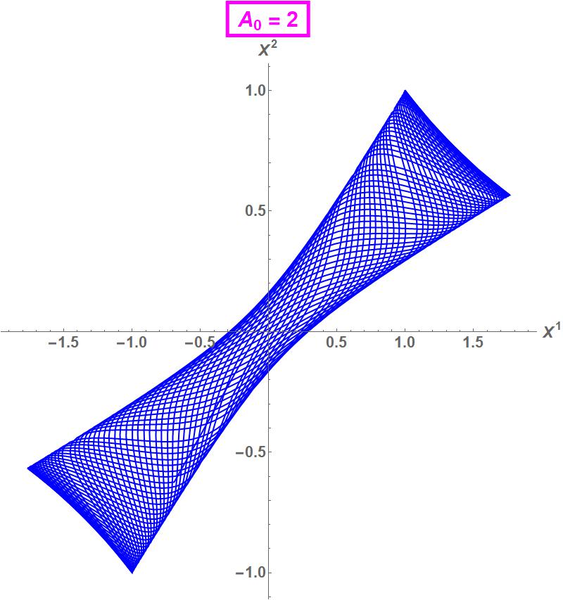
  Figure 1: In a weak linearly polarized periodic (LPP) wave, (3.4), the transverse coordinate ${\bm{X}}(U)$ oscillates in a bounded “bow tie”-shaped domain. The initial conditions are $\dot{X}^{+}(U\!=\!0)=\dot{X}^{-}(U\!=\!0)=0$ (at rest for $U\!=\!0$), at initial position $X^{+}(U\!=\!0)=1,\,X^{-}(U\!=\!0)=0$.

  A sufficiently strong wave breaks up the bound motion.

• The general form in eqn. (3.2b) allows however also for more general profiles, and now we turn to waves with circularly polarized periodic profile (CPP), considered before e.g. in POLPER ,

  $$K=\big{(}K_{ij})=\frac{A_{0}}{2}\left(\begin{array}[]{lr}\cos 2U&\sin 2U\\ \sin 2U&-\cos 2U\end{array}\right)\qquad A_{0}=\mathop{\rm const}\nolimits>0\,.$$ (3.5)

The transverse eqns of motion, ${\bm{X}}^{\prime\prime}=K{\bm{X}},$ should be supplemented by appropriate initial conditions. In the sandwich case one usually considers particles which are at rest in the before zone. But a periodic wave has no before zone, and here we propose the initial condition ,

$$\text{rest\ at\ $U=0$}\quad\text{i.e.,}\quad{\bm{X}}^{\prime}(0)=0.$$ (3.6)

Then numerical calculations POLPER yield Fig.2 : for a sufficiently weak wave all motions remain confined to a toroidal region; for a strong wave the trajectory becomes instead unbounded : the particle is ejected.

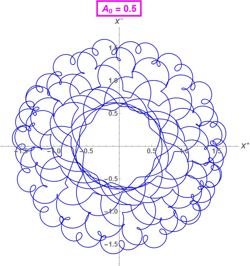
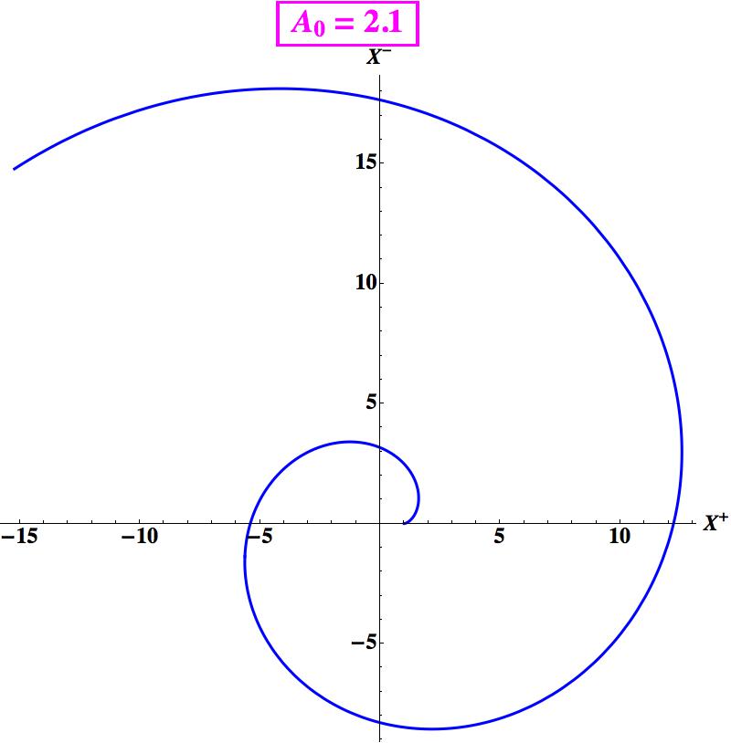
(i)                                                            (ii)

Figure 2: (i) In a sufficiently weak circularly polarized gravitational wave (3.5) the transverse trajectory of a particle initially at rest remains confined in a toroidal region. (ii) For a strong wave the trajectory becomes unbounded. The initial conditions are $\dot{X}^{+}(U=0)=\dot{X}^{-}(U=0)=0$ and $X^{+}(U=0)=1,\,X^{-}(U=0)=0.$

Below we show that the problem admits an exact analytic solution. Following a suggestion of Kosinski Kosinski , the first step is to switch to a rotating frame by setting

$$\left(\begin{array}[]{c}X^{+}\\ X^{-}\end{array}\right)=\left(\begin{array}[]{rcr}\cos U&&-\sin U\\ \sin U&&\cos U\end{array}\right)\left(\begin{array}[]{c}Y^{+}\\ Y^{-}\end{array}\right).$$ (3.7)

In terms of the new coordinates $Y^{\pm}$ the harmonic force becomes $U$-independent — at the price of introducing the cross terms $\mp 2(Y^{\mp})^{\prime}$ ,

$$\;\;\displaystyle{(Y^{\pm})^{\prime\prime}\mp 2(Y^{\mp})^{\prime}-{\Omega^{2}_{\pm}}\,Y^{\pm}=0\,\quad\text{where}\quad\Omega_{\pm}^{2}={1\pm A_{0}/2}\,.}\;\;$$ (3.8)

Our initial condition (3.6) is valid in Brinkmann-coordinates (3.2a) ; from Eqn. (3.7) we infer instead

$${\bm{Y}}^{\prime}(0)=\left(\begin{array}[]{cc}0&1\\ -1&0\end{array}\right){\bm{Y}}_{0}\,=\left(\begin{array}[]{cc}0&1\\ -1&0\end{array}\right){\bm{X}}_{0}\,,$$ (3.9)

i.e., ${\bm{Y}}^{\prime}(0)$ is obtained from ${\bm{Y}}(0)={\bm{X}}_{0}\,$ by a $90$-degree rotation, which corresponds precisely to rotating the coordinate system.

The eqns of motion can be conveniently solved by chiral decomposition Alvarez ; ZGH . Eqns. (3.8) belong indeed to a Hamiltonian system in the plane, whose phase space is thus $4$ dimensional ; it has coordinates $Y^{\pm}$ and $\Pi^{\pm}={(Y^{\pm})}^{\prime}$. Then the idea is to choose “smart” phase-space coordinates we denote here by $Z_{+}^{a},\,Z_{-}^{b},\,a,b=1,2$ such that the system decouples onto uncoupled $1D$ oscillators Alvarez ; ZGH . Searching for real coefficients $\alpha_{\pm}$ and $\beta_{\pm}$,

$$\Pi^{+} =\alpha_{+}Z_{+}^{2}+\alpha_{-}Z_{-}^{2}\,, \Pi^{-} =-\beta_{+}Z_{+}^{1}-\beta_{-}Z_{-}^{1}\,,$$ (3.10a)

$$Y^{+} =Z_{+}^{1}+Z_{-}^{1}\,, Y^{-} =Z_{+}^{2}+Z_{-}^{2}\,,$$ (3.10b)

in terms of which both the symplectic form and the Hamiltonian separate, we find that for $\alpha_{+}=1,\,\alpha_{-}=\Omega_{-}^{2},\,\beta_{+}=\Omega_{+}^{2},\,\beta_{-}=1,$ for example ,

$$\sigma =\sigma_{+}-\sigma_{-}=-\frac{A_{0}}{2}\Big{[}dZ_{+}^{1}\wedge dZ_{+}^{2}-dZ_{-}^{1}\wedge dZ_{-}^{2}\Big{]},$$ (3.11a)

$$H =H_{+}-H_{-}=\frac{A_{0}}{4}\Big{[}\big{(}\Omega_{+}^{2}Z_{+}^{1}Z_{+}^{1}+Z_{+}^{2}Z_{+}^{2}\big{)}-\big{(}Z_{-}^{1}Z_{-}^{1}+\Omega_{-}^{2}Z_{-}^{2}Z_{-}^{2}\big{)}\Big{]}.$$ (3.11b)

The relative negative signs between the terms reflect here the chiral nature : the two oscillators turn in the opposite direction ZHAGK . The Poisson brackets associated with the symplectic structure (3.11a) are,

$$\{Z_{+}^{1},Z_{+}^{2}\}=\frac{2}{A_{0}},\qquad\{Z_{-}^{1},Z_{-}^{2}\}=-\frac{2}{A_{0}},\qquad\{Z_{+}^{1},Z_{-}^{2}\}=\{Z_{+}^{2},Z_{-}^{1}\}=0.$$ (3.12)

Working out the Hamilton equations, we end up with uncoupled oscillator equations,

$${(Z_{\pm}^{a})}^{\prime\prime}+\Omega_{\pm}^{2}Z_{+}^{a}=0,$$ (3.13)

($a=1,2$), whose solutions (when none of the $\Omega_{\pm}$ vanishes ), are,

$$Z_{+}^{1} =A\cos(\Omega_{+}U)+B\sin(\Omega_{+}U),$$ (3.14a)

$$Z_{+}^{2} =-\Omega_{+}\Big{(}A\sin(\Omega_{+}U)-B\cos(\Omega_{+}t)\Big{)},$$ (3.14b)

$$Z_{-}^{1} =C\cos(\Omega_{-}U)+D\sin(\Omega_{-}U),$$ (3.14c)

$$Z_{-}^{2} =-\frac{1}{\Omega_{-}}\Big{(}C\sin(\Omega_{-}U)-D\cos(\Omega_{-}U)\Big{)},$$ (3.14d)

where $A,B,C,D$ are constants. Proceeding backwards we obtain, using (3.10b),

$$Y^{+}(U) =\qquad\;\,A\cos\Omega_{+}U+B\sin\Omega_{+}U\;\;\;+\qquad C\cos\Omega_{-}U+D\sin\Omega_{-}U\,,$$ (3.15a)

$$Y^{-}(U) =-\Omega_{+}(A\sin\Omega_{+}U-B\cos\Omega_{+}U)\;-\;\dfrac{1}{\Omega_{-}}(C\sin\Omega_{-}U-D\cos\Omega_{-}U)\,.$$ (3.15b)

For a weak wave i.e. such whose amplitude is $A_{0}<2$ both frequencies $\Omega_{\pm}$ in (3.8) are real, implying that the motion, although complicated, remains bounded. A typical trajectory is shown in Figs.7 and 8 of POLPER . However for a strong wave with amplitude $A_{0}>2$ one (and only one) of the $\Omega_{\pm}$ becomes imaginary and the corresponding motion is unbounded: a sufficiently strong wave ejects the particle and makes it escape. Between those two regimes i.e., for $A_{0}=2$, one of the $\Omega$’s vanishes, and the motion in the corresponding direction is free; we recover eqn. # (5.11) of POLPER , illustrated in Fig.9 of that paper.

The solutions (3.15) are plotted for $A_{0}<2$ in Fig.3. The one which has smaller real (or imaginary) frequency can be viewed (somewhat arbitrarily) as a guiding center, around which the one with the larger frequency winds around. For $A_{0}=2$ one of the frequencies vanishes, $\Omega_{-}=0$, and the $Y$-trajectory is an ellipse drifting with constant speed ZGH ; ZHAGK .

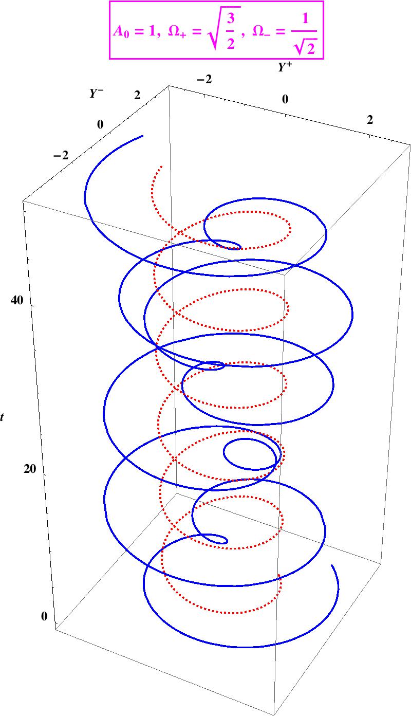
Figure 3: In the circularly polarized periodic gravitational wave (3.5) the trajectory unfolded into “time”(in heavy blue) winds about the guiding center (dotted in red). If the wave is weak, $A_{0}<2$, the trajectory remains bounded, projecting to the plane consistently with Fig.2.

A further rotation (3.7) backward would yield the trajectories $X^{\pm}(U)$.

As noticed by Ilderton Ilderton , eqns (3.8) are actually identical to eqns. # (10a-b) of Białynicki-Birula for a charged particle in the field of an electromagnetic vortex BBvort , and (3.15) above just reproduces his solution # (14) – with some additional insight, though. The relation will be further discussed elsewhere.

So far we studied classical motions only. However the system could readily be quantized, courtesy of the chiral decomposition Alvarez ; ZGH ; ZHAGK ; BBvort . The Poisson brackets (3.12) are promoted to commutation relations,

$$[Z_{+}^{i},Z_{+}^{j}]=\frac{2i\hbar}{A_{0}}\epsilon^{ij},\qquad[Z_{-}^{i},Z_{-}^{j}]=-\frac{2i\hbar}{A_{0}}\epsilon^{ij},$$ (3.16)

where we denoted, with a light abuse of notations, the classical and quantum observables by the same symbols. Creation and annihilation operators can now be introduced,

$$a^{\dagger} =\sqrt{\frac{A_{0}\Omega_{+}}{4}}\left(Z_{+}^{1}-\frac{i}{\Omega_{+}}Z_{+}^{2}\right),\qquad a=\sqrt{\frac{A_{0}\Omega_{+}}{4}}\left(Z_{+}^{1}+\frac{i}{\Omega_{+}}Z_{+}^{2}\right)\,,$$ (3.17a)

$$b^{\dagger} =\sqrt{\frac{A_{0}\Omega_{-}}{4}}\left(Z_{-}^{2}-\frac{i}{\Omega_{-}}Z_{-}^{1}\right),\qquad b=\sqrt{\frac{A_{0}\Omega_{-}}{4}}\left(Z_{-}^{2}+\frac{i}{\Omega_{-}}Z_{-}^{1}\right)\,,$$ (3.17b)

whose non-vanishing commutators are, by (3.16),

$$[a,a^{\dagger}]=1=[b,b^{\dagger}].$$ (3.18)

In their terms the Hamiltonian is,

$$H=\left(\Omega_{+}\big{(}a^{\dagger}a+\frac{1}{2}\big{)}-\Omega_{-}\big{(}b^{\dagger}b+\frac{1}{2}\big{)}\right).$$ (3.19)

The number operators $a^{\dagger}a$ and $b^{\dagger}b$ commute and have [$\hbar$-times] integer eigenvalues. The bound-state spectrum is therefore,

$$E_{n_{+},n_{-}}=\hbar\Big{[}\Omega_{+}\big{(}n_{+}+{\scriptstyle{\frac{1}{2}}}\big{)}-\Omega_{-}\big{(}n_{-}+{\scriptstyle{\frac{1}{2}}}\big{)}\Big{]}\qquad n_{\pm}=0,1\dots$$ (3.20)

Let us observe that the spectrum is not bounded from below, consistently with the relative minus sign of $H_{+}$ and $H_{-}$ in the Hamiltonian (3.11b) reflecting the shape of the saddle potential.

4 Sturm-Liouville problem & switching to BJR

The key to study the memory effect for gravitational waves is to solve the Sturm-Liouville equation with an auxiliary condition ShortLong ; Torre ; SLC ,

$${P}^{\prime\prime}(U) =K(U)P(U),$$ (4.1a)

$$P(U)^{T}{P}^{\prime}(U) =\big{(}{P}^{\prime}(U)\big{)}^{T}P(U).$$ (4.1b)

This system should be supplemented by initial conditions. Let us recall that in the sandwich case, for which the wave vanishes outside an interval $[U_{i},U_{f}]$, we required in the before zone $U\leq U_{i}$ the initial conditions

$$P(U)=\mathbb{I},\quad\&\quad P^{\prime}(U)=0\quad\text{for}\quad U\leq U_{i}\,.$$ (4.2)

Below we extend our study to the periodic case, which has no before zone. First we note that having solved the SL eqn. (4.1) for the $2\times 2$ matrix $P(U)$,

1. allows us to switch to Baldwin-Jeffery-Rosen (BJR) coordinates $({\bm{x}},u,v)$ : setting

   $$X^{i} =P^{ij}(u)\,x^{j}\,,$$ (4.3a)

   $$U =u\,$$ (4.3b)

   $$V =v-\frac{1}{4}\,y^{i}{(G^{ij})}^{\prime}(u)\,x^{j}\,,\quad\text{where}\quad G=P^{T}P\,$$ (4.3c)

   carries the metric (3.2a) with $g_{ij}=\delta_{ij}$ to the BJR form

   $$G_{ij}(u)dx^{i}dx^{j}+2dudv\,.$$ (4.4)

2. The metric admits a $5$ parameter isometry BoPiRo ; Sou73 ; exactsol ; Sippel ; Torre ; Carroll4GW . The system is in particular symmetric with respect to translations and boosts, with associated conserved momenta

   $$p_{i} =G_{ij}\dot{x}^{j}$$ (4.5a)

   $$k_{i} =x_{i}(u)-H_{ij}(u)\,p_{j}$$ (4.5b)

   where $H(u)$ is the $2\times 2$ matrix $H(u)=\displaystyle\int_{u_{0}}^{u}{\!G^{-1}(w)dw}$ Sou73 ; Carroll4GW ; ShortLong  .

3. Remember that in the sandwich case the usual assumption is that the particle is at rest in the before zone, ${\bm{X}}^{\prime}(U)=0$ for $U<U_{i}$. Then exporting to BJR by (4.3a),

   $${\bm{x}}=P^{-1}{\bm{X}}\quad\Rightarrow\quad{\bm{x}}^{\prime}(0)=\big{(}-P^{-1}P^{\prime}(P^{-1}\big{)}(0){\bm{X}}(0)+(P^{-1}){\bm{X}}^{\prime}(0)=0\,,$$

   and thus the BJR coordinate also has vanishing initial velocity, ${\bm{x}}^{\prime}(u)=0$. Consequently the linear momentum vanishes, ${\bm{p}}=0$ by (4.5a) ; then (4.5b) implies that ${\bm{x}}(u)={\bm{x}}_{0}$ for all $u$. Returning to Brinkmann coordinates allows us to conclude, using (4.2), that the trajectory is simply

   $$\;\;\displaystyle{{\bm{X}}(U)=P(U){\bm{X}}_{0}\,.}\;\;$$ (4.6)

   Now we extend our theory by replacing the initial conditions (4.2) by requiring that it holds at a chosen initial moment, e.g.,

   $$\;\;\displaystyle{P(0)=\mathbb{I},\quad\&\quad P^{\prime}(0)=0\,.}\;\;$$ (4.7)

   Then (4.6) remains true also in our case : the SL eqns (4.1) imply that it satisfies the equations of motion with the initial conditions ${\bm{X}}(0)={\bm{X}}_{0}$ and ${\bm{X}}^{\prime}(0)=0$. Conversely, following the same argument as in the sandwich case, we observe that inverting (4.3a) shows that ${\bm{X}}^{\prime}(0)=0$ implies ${\bm{x}}^{\prime}(0)=0$ and therefore ${\bm{p}}=0$ by (4.5a) from which (4.5b) allows us to infer ${\bm{x}}(u)={\bm{x}}_{0}=\mathop{\rm const}\nolimits$, so that (4.3a) yields once again (4.6).

4.1 Linearly Polarized Periodic (LPP) waves

In the linearly polarized case (3.4) Mathematica tells us that eqn (4.1a) can be solved : Using the shorthands $c_{A_{0}}(U)\equiv C({0,A_{0}},U)$ and $s_{A_{0}}(U)\equiv S({0,A_{0}},U)$  cf. sec. 2, we get,

$$P(U)=\left(\begin{array}[]{ccc}A_{11}\,c_{A_{0}}(U)+B_{11}\,s_{A_{0}}(U)&&A_{12}\,c_{A_{0}}(U)+B_{12}\,s_{A_{0}}(U)\\[6.0pt] A_{21}\,c_{-A_{0}}(U)+B_{21}\,s_{-A_{0}}(U)&&A_{22}\,c_{-A_{0}}(U)+B_{22}\,s_{-A_{0}}(U)\end{array}\right)$$ (4.8)

with $A_{ij}$ and $B_{ij}$ constants of integration. Then eqn (4.1b) yields the compatibility constraints

$$A_{11}B_{12}=A_{12}B_{11}\qquad\&\qquad A_{22}B_{21}=A_{21}B_{22}.$$ (4.9)

Assuming that, e.g., $A_{11}\neq 0$ and $A_{22}\neq 0$ we obtain $B_{12}$ and $B_{21}$. The solution thus depends on $6$ integration constants. Then it follows that from the parity-properties of the Mathieu functions that the initial condition ${\bm{X}}^{\prime}(U)=0$ in (3.6) can only be satisfied if all $B_{ij}$ vanish (and then the auxiliary conditions (4.9) hold also). Then, consistently with eqn (IV.3) of POLPER , the trajectory is given by pure Mathieu cosines with labels $\pm A_{0}$ and coefficients depending on the initial conditions,

$$X^{\pm}(U)=D^{\pm}\,c_{{\pm}A_{0}}(U)\,,$$ (4.10)

where the constants $D^{\pm}$ are determined by the $A_{ij}$ in (4.8) and the initial position ${\bm{X}}_{0}$.

4.2 Circularly Polarized Periodic (CPP) waves

Now we turn to the circularly polarized wave (3.5). Switching to a rotating frame by (3.7) allows us to present the metric as,

$$ds^{2} =d{\bm{Y}}^{2}+2dU\Big{(}dV+A\Big{)}\;-\;2\Psi dU^{2},$$ (4.11a)

$$A =-Y^{-}dY^{+}+Y^{+}dY^{-}\,,\qquad\Psi=-{\scriptstyle{\frac{1}{2}}}\Big{(}\Omega_{+}^{2}(Y^{+})^{2}+\Omega_{-}^{2}(Y^{-})^{2}\Big{)}.$$ (4.11b)

The only non-vanishing component of the Ricci tensor of (4.13) is

$$R_{UU}=-{\partial}_{U}(\mbox{\boldmath$\nabla$}\cdot{\bm{A}})-{\scriptstyle{\frac{1}{2}}}B^{2}-\Delta\Psi$$ (4.12)

where $B={\partial}_{i}A_{j}-{\partial}_{j}A_{i}$. Ricci-flatness is thus confirmed for (4.11) .

This metric is consistent with the Bargmann description of a particle with charge = mass in a combined anisotropic oscillator plus a “magnetic” (alias Coriolis) field. The appearance of the new metric component implies that the potential term $\Psi$ alone does not contain all information. The metric (4.11) has the form of a pp metric sometimes called “gyratonic” ,

$$d{\bm{Y}}^{2}+2dU\big{(}dV+A\big{)}-2\Psi\,dU^{2},$$ (4.13)

where now $\Psi=-{\scriptstyle{\frac{1}{2}}}H_{ij}Y^{i}Y^{j}$ and where the $1$-form $A=A_{\mu}dY^{\mu}$ is a vector potential. It has a gauge freedom: $A_{i}\rightarrow A_{i}-{\partial}_{i}\Lambda$ can be compensated by the “vertical” coordinate transformation $V\rightarrow V+\Lambda({\bm{Y}})$.

Switching to BJR coordinates by replacing ${\bm{X}}$ by ${\bm{Y}}$ and ${\bm{x}}$ by ${\bm{y}}$ in (4.3a), the new term in (4.13) becomes

$$2dUA_{j}(Y)dY^{j}=2du\,d\left(A_{j}(Y)Y^{j}\right)-2du\,{\partial}_{i}A_{j}(Y)dY^{i}Y^{j}=$$

$$2du\,d\left(A_{j}(Y)Y^{j}\right)-2\left({(P^{\prime})}^{T}{\partial}AP\right)^{(ij)}\!\!y^{i}y^{j}du^{2}-2\big{(}P^{T}{\partial}AP\big{)}^{ij}y^{j}du\,dy^{i}\,,$$

where we used the shorthand ${\partial}A$ for the matrix $[{\partial}A_{j}/{\partial}Y_{i}]$. The first term here can be reabsorbed into the $V$-change in (4.3c),

$$V=v-\frac{1}{4}y^{i}{(a^{ij})}^{\prime}(u)y^{j}-2A_{j}(Y)P^{jk}y^{k}\,.$$

The two other terms modify the Sturm-Liouville equations (4.1) : the auxiliary condition (4.1b) becomes

$$P^{T}{P^{\prime}}-{(P^{\prime})}^{T}P=2\left(P^{T}{\partial}AP\right)\,,$$

whose consistency requires ${\partial}A=-{\partial}A^{T}$. Then the SL equation (4.1a) becomes

$$-\frac{1}{2}\left({\big{(}P^{\prime\prime}\big{)}}^{T}P+P^{T}P^{\prime\prime}\right)+P^{T}HP={(P^{\prime})}^{T}{\partial}AP-P^{T}{\partial}A{P^{\prime}}.$$

When ${\partial}_{U}({\partial}A)=0$, both equations are solved by ${P}^{\prime\prime}=KP+2{\partial}A{P^{\prime}}\,.$ To sum up, changing our notations to emphasise that the new system concerns the metric obtained after applying the rotational trick, ${\bm{X}}\to{\bm{Y}}\,,\,K=\big{(}K_{ij}\big{)}\to H=\big{(}H_{ij}\big{)}$ and $P\rightarrow Q$, eqns (4.3) for the Brinkmann $\Leftrightarrow$ BJR transcription should be replaced by

$$Y^{i} =Q^{ij}(u)y^{j}\,,$$ (4.14a)

$$U =u\,$$ (4.14b)

$$V =v-\frac{1}{4}y^{i}{(G^{ij})}^{\prime}y^{j}-2A_{j}\,Q^{jk}y^{k}\,,\qquad G=Q^{T}Q\,.$$ (4.14c)

Note that the eqns (4.3a) are formally unchanged while (4.3c) picks up a new term, however the SL eqns to be solved are now rather

$$Q^{\prime\prime} =HQ+2{\partial}A\,{Q^{\prime}}\,,$$ (4.15a)

$${\partial}A =-{\partial}A^{T}\,,$$ (4.15b)

$${\partial}_{U}({\partial}A) =0\,.$$ (4.15c)

Spelling out our formulae for the circularly polarized periodic wave, from (4.11) we infer that

$${\partial}A=\left(\begin{array}[]{cc}0&1\\ -1&0\end{array}\right),\qquad H=\left(\begin{array}[]{cc}\Omega_{+}^{2}&0\\ 0&\Omega_{-}^{2}\end{array}\right)\,,$$ (4.16)

which are both $U$-independent. Thus our modified Sturm-Liouville equation becomes

$$\;\;\displaystyle{Q^{\prime\prime}+2\left(\begin{array}[]{cc}0&-1\\ 1&0\end{array}\right)Q^{\prime}-\left(\begin{array}[]{cc}\Omega_{+}^{2}&0\\ 0&\Omega_{-}^{2}\end{array}\right)\,Q=0\,\\ }\;\;$$ (4.17)

which is precisely eqn. (3.8) with the vector ${\bm{Y}}$ replaced by the $2\times 2$ matrix $Q$. Replacing ${\bm{X}}$ by ${\bm{Y}}$ in (4.6), it follows that

$$\;\;\displaystyle{{\bm{Y}}(U)=Q(U){\bm{Y}}_{0}}\;\;$$ (4.18)

is a solution of the equations of motion (3.8). Moreover, the initial condition (3.9) is satisfied provided,

$$\;\;\displaystyle{Q(0)=\mathbb{I}\,,\qquad Q^{\prime}(0)=\left(\begin{array}[]{cc}0&1\\ -1&0\end{array}\right)\,.}\;\;$$ (4.19)

Our new equation (4.17) has constant coefficients and can be solved analytically. Putting $Q=(Q_{ij})$ (4.17) is mapped indeed into two sets of equations of type (3.8), with the identifications $Q_{11}\leftrightarrow Y^{+}$, $Q_{21}\leftrightarrow Y^{-}$, $Q_{12}\leftrightarrow Y^{+}$, $Q_{22}\leftrightarrow Y^{-}$ : the columns of $Q$ are vectors of the form $\left(\begin{array}[]{c}Y^{+}\\ Y^{-}\end{array}\right)$ both of which satisfy (3.8). Therefore the general solution is, by (3.15), a combination with eight constants $A_{i},\dots,D_{i}$, $i=1,2$ cf. (4.8),

$$Q_{11}(U) =\,A_{1}\cos\Omega_{+}U+B_{1}\sin\Omega_{+}U+C_{1}\cos\Omega_{-}U+D_{1}\sin\Omega_{-}U\,,$$ (4.20a)

$$Q_{21}(U) =-\Omega_{+}(A_{1}\sin\Omega_{+}U-B_{1}\cos\Omega_{+}U)\;-\;\dfrac{1}{\Omega_{-}}(C_{1}\sin\Omega_{-}U-D_{1}\cos\Omega_{-}U)\,,$$ (4.20b)

$$Q_{12}(U) =\,A_{2}\cos\Omega_{+}U+B_{2}\sin\Omega_{+}U+C_{2}\cos\Omega_{-}U+D_{2}\sin\Omega_{-}U\,,$$ (4.20c)

$$Q_{22}(U) =-\Omega_{+}(A_{2}\sin\Omega_{+}U-B_{2}\cos\Omega_{+}U)\;-\;\dfrac{1}{\Omega_{-}}(C_{2}\sin\Omega_{-}U-D_{2}\cos\Omega_{-}U)\,,$$ (4.20d)

The number of constants is halved by the initial condition (4.19) which require,

$$C_{1}=1-\Omega_{+}^{2}A_{1}\,,\;\;D_{1}=-\frac{\Omega_{+}}{\Omega_{-}}B_{1}\,,\;\;C_{2}=-\Omega_{+}^{2}A_{2}\,,\;\;D_{2}=\frac{1}{\Omega_{-}}-\frac{\Omega_{+}}{\Omega_{-}}B_{2}\,.$$

Requiring in addition also $Q(0)=\mathbb{I}$ which follows from (4.18) eliminates all constants with the exception of $B_{2}=\Omega_{+}^{-1}$, leaving us with

$$Q=\left(\begin{array}[]{ccc}\cos(\Omega_{-}U)&&\frac{\displaystyle{\sin(\Omega_{+}U)}}{\Omega_{+}}\\[10.0pt] -\frac{\displaystyle{\sin(\Omega_{-}U)}}{\Omega_{-}}&&\cos(\Omega_{+}U)\end{array}\right)\,.$$ (4.21)

5 Ion Traps in 3D

5.1 Paul Trap in 3D

Real traps are $3$-dimensional : ions are Paul-trapped by a time-dependent quadrupole potential, written, in appropriate units, as PaulNobel ; Blumel ,

$$\Phi=\frac{1}{2}\big{(}a+2q\cos 2U\big{)}\Big{(}(X^{+})^{2}+(X^{-})^{2}-2z^{2}\Big{)},$$ (5.1)

where $a$ and $q$ are parameters and we used again the notation $U=\omega t/2$. (5.1) is clearly an axi-symmetric anisotropic oscillator potential with time-dependent frequencies. The motion of an ion is described therefore by three uncoupled Mathieu equations,

$$(X^{\pm})^{\prime\prime}+\,\big{(}a+2q\cos 2U\big{)}\,X^{\pm} =\;0,$$ (5.2a)

$$\quad z^{\prime\prime}\;-\;2\big{(}a+2q\cos 2U\big{)}\,z =\;0\,.$$ (5.2b)

The interaction in the $X^{\pm}$ plane is attractive, while the one in the $z$ direction is repulsive and has a factor $2$. The oscillating term produces bounded motions in an appropriate range of parameters. For details the reader is referred to the literature, e.g. Blumel . Some bounded trajectories are shown in Figs.4.

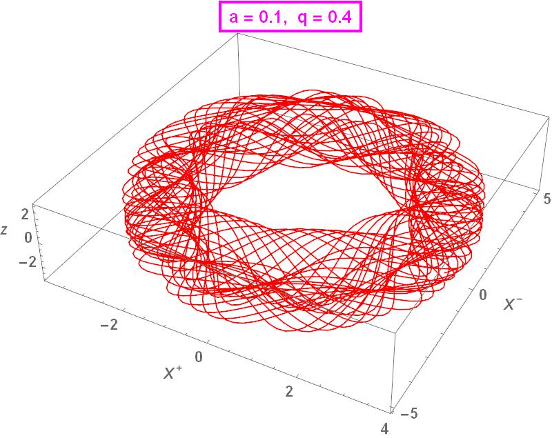
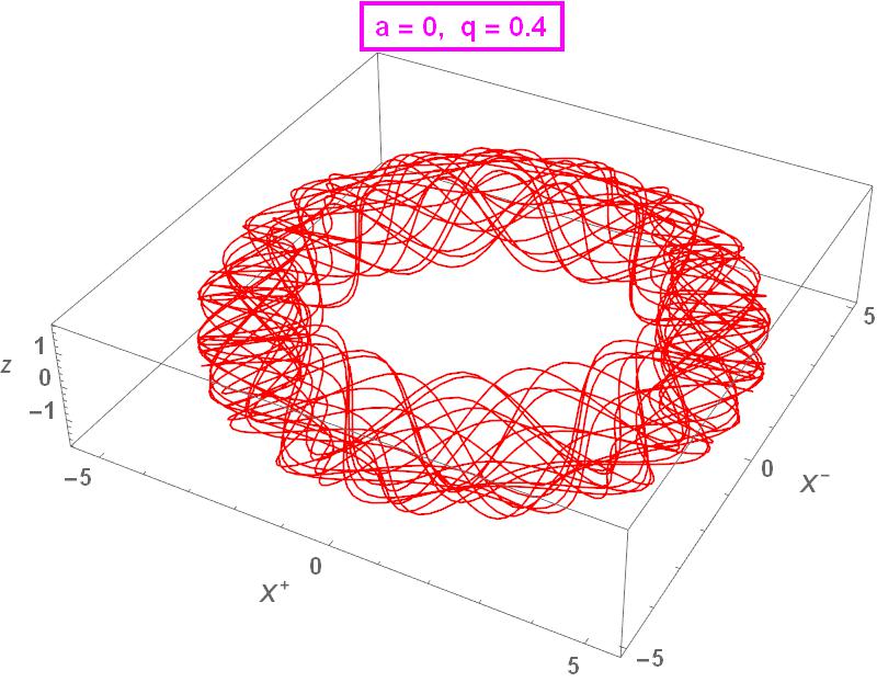
(i)                                                  (ii)

Figure 4: Motion in a $3D$ Paul Trap for (i) $a=0.1$ (axial symmetry) (ii) $a=0$ (periodic profile). The initial conditions $X^{+}(0)=0,\,\dot{X}^{+}(0)=1,\,X^{-}(0)=5,\,\dot{X}^{-}(0)=0,\,z(0)=0,\,\dot{z}(0)=1$.

The $3D$ Paul Trap can again be lifted to Bargmann space – but one in $5D$. The recipe is the same as before Bargmann : the Bargmann metric is (3.2a) but now we have $3$ transverse components ; the $UU$ component is $-2\Phi(X^{\pm},z,U)$ given in (5.1). The quadratic form is traceless and therefore the metric still satisfies the vacuum Einstein equations $R_{\mu\nu}=0$ : it is a gravitational wave in $5D$.

5.2 Penning Trap

A similar however different ion trap was proposed by Dehmelt who called it the Penning Trap DehmeltNobel ; Brown ; Blaum (and who shared for it the Nobel prize with Paul). It combines an anisotropic but time-independent quadrupole potential with a uniform (constant) magnetic field ${\bm{B}}=B\,\hat{z}$ directed along the $z$ axis,

$$\Psi(Y^{+},Y^{-},z) =-\big{(}\frac{\omega_{z}}{2}\big{)}^{2}\,\Big{(}(Y^{+})^{2}+(Y^{-})^{2}-2z^{2}\Big{)},$$ (5.3a)

$$A_{+} =-{\scriptstyle{\frac{1}{2}}}B{Y^{-}},\quad A_{-}={\scriptstyle{\frac{1}{2}}}B{Y^{+}},\quad A_{z}=0\,.$$ (5.3b)

The Lagrangian

$$L=\frac{1}{2}\dot{{\bm{Y}}}^{2}+\frac{\omega_{c}}{2}(\dot{Y}^{-}Y^{+}-\dot{Y}^{+}Y^{-})+\frac{1}{4}\omega_{z}^{2}({\bm{Y}}^{2}-2z^{2})\,,$$ (5.4)

where $\omega_{c}=B$ in our units is the cyclotron frequency , yields, for a particle of unit charge and mass,

$$\ddot{Y}^{\pm}\mp\omega_{c}\dot{Y}^{\mp}-\dfrac{1}{2}\omega_{z}^{2}\,{Y^{\pm}}=0\,$$ (5.5a)

$$\ddot{z}+\omega_{z}^{2}z=0\,$$ (5.5b)

cf. eqns. # (2.5)-(2.7) of ref. Kretzschmar .

Let us observe for further reference that the upper eqns, (5.5a), are reminiscent of the circularly polarized periodic (CPP) form (3.8) [as suggested by our notations], while the $z$-equation is that of a decoupled harmonic oscillator. In terms of the complex coordinate $\Upsilon=Y^{+}+iY^{-}$ eqn. (5.5a) is solved by Kretzschmar ,

$$\Upsilon_{\pm}(t)=e^{-i\gamma_{\pm}t},\qquad\gamma_{\pm}={\scriptstyle{\frac{1}{2}}}\big{(}\omega_{c}\pm\sqrt{\omega_{c}^{2}-2\omega_{z}^{2}}\big{)}.$$ (5.6)

The constants $\gamma_{+}$ and $\gamma_{-}$ here are the modified cyclotron frequency and the magnetron frequency, respectively. Periodic solutions require $\omega_{c}^{2}-2\omega_{z}^{2}>0$. Solutions are shown in Fig. 5 ; bound motions arise when $\omega_{z}^{2}>0$.

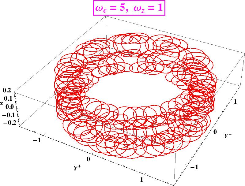
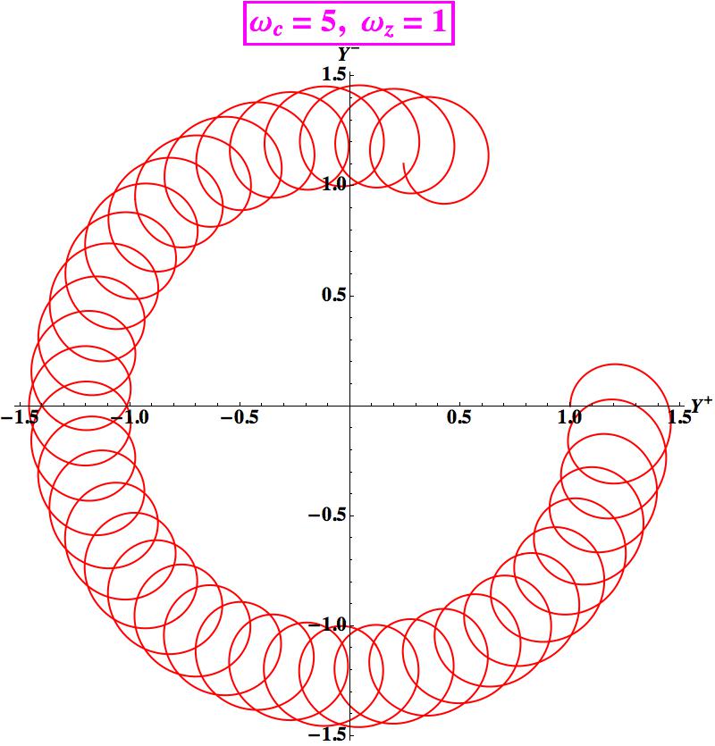
(i)                                                                (ii)

Figure 5: Trajectory of a charged particle in a Penning Trap (i) in $3D$ (ii) its projection on the $Y^{\pm}$ plane. The initial conditions are $Y^{+}(0)=1.0,~{}\dot{Y}^{+}(0)=0.0,~{}Y^{-}(0)=0,~{}\dot{Y}^{-}(0)=1.0,~{}z(0)=0,~{}\dot{z}(0)=0.2$.

In experimentally realistic cases $\omega_{c}>>\omega_{z}$ Brown ; Kretzschmar . However a special case arises when the Penning trap has equal modified-cyclotron and magnetron frequencies,

$$\gamma_{+}=\gamma_{-}={\scriptstyle{\frac{1}{2}}}\omega_{c},\qquad\text{i.e.\ for}\qquad\Delta=\left(\frac{\omega_{z}}{\omega_{c}}\right)^{2}-\frac{1}{2}=0.$$ (5.7)

Then both motions in (5.6) coincide (are purely cyclotronic) whereas the new independent solution spirals outward as shown in Fig.6, reminiscent of the maximally anisotropic case $\Omega_{-}=0$ in Fig.9 of POLPER ,

$$\Upsilon_{0}^{(per)}(t)=e^{-i{\scriptstyle{\frac{1}{2}}}\omega_{c}t},\qquad\Upsilon_{0}^{(esc)}(t)=t\,e^{-i{\scriptstyle{\frac{1}{2}}}\omega_{c}t}\,.$$ (5.8)

The toroidal region shrinks to a circle and we get also a new, escaping solution. The general solution of the $3D$ system (5.5), a combination of those in (5.6) completed with $z=E\cos(\omega_{z}\,t)+F\cos(\omega_{z}\,t)$, can be also obtained by chiral decomposition.

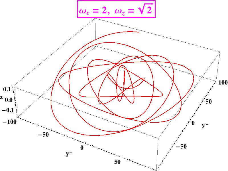
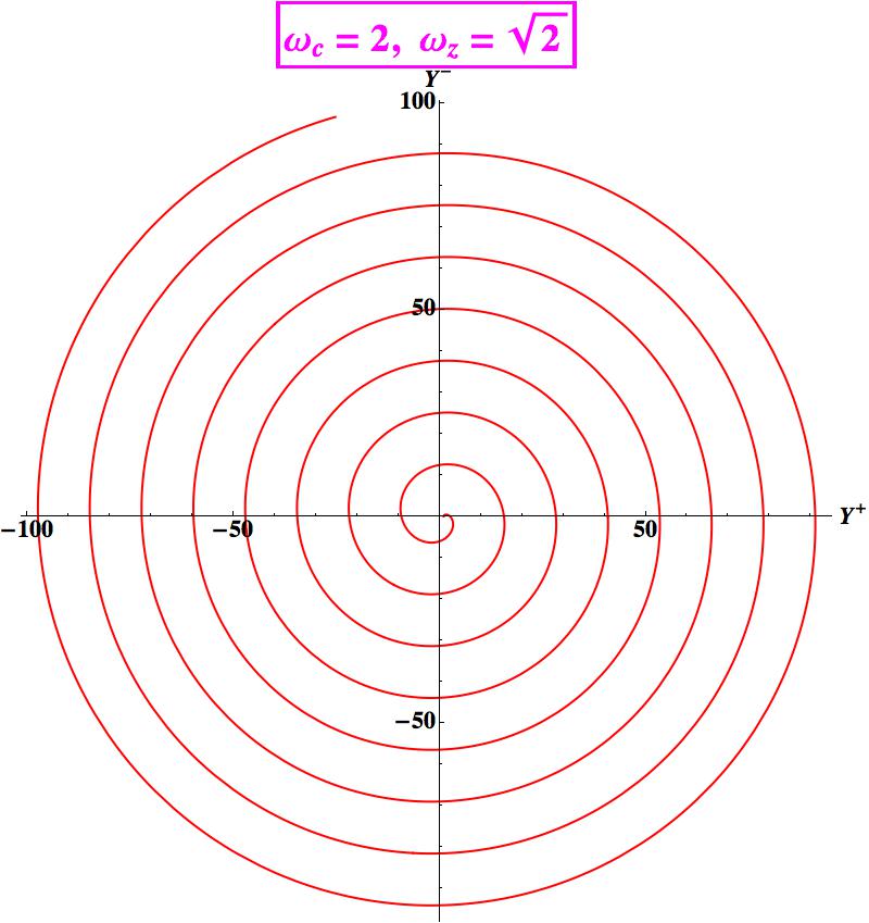
(i)                                                      (ii)

Figure 6: In the fine-tuned case (5.7) and for initial conditions $Y^{+}(0)=1.0,~{}\dot{Y}^{+}(0)=0.0,~{}Y^{-}(0)=0,~{}\dot{Y}^{-}(0)=1.0,~{}z(0)=0,~{}\dot{z}(0)=0.2$, the $2d$ projection (ii) of the $3d$ trajectory (i) spirals outward with expanding radius. The $z$ coordinate oscillates with frequency $\omega_{z}=\omega_{c}/\sqrt{2}$.

For a discussion of the quantum aspects the reader is referred, e.g. Brown to for details. Here we just mention that the spectrum is Brown ,

$$E_{(n_{+},n_{-},k)}=\hbar\bigg{[}\gamma_{+}\big{(}n_{+}+{\scriptstyle{\frac{1}{2}}}\big{)}-\gamma_{-}\big{(}n_{-}+{\scriptstyle{\frac{1}{2}}}\big{)}+\omega_{z}\big{(}k+{\scriptstyle{\frac{1}{2}}}\big{)}\bigg{]},\qquad n_{\pm},k=0,1,\dots$$ (5.9)

as it can also be confirmed by the chiral method. In the special case (5.7) the bound-state spectrum is that of the $z$ component alone, consistently with (5.8) and Fig.6 .

Now we turn to the GW aspect of 3D traps. As said above, Paul Traps correspond to linearly polarized periodic (LPP) waves; now we inquire if the analogy can be extended by relating the Penning trap to CPP waves. We first recall how a non-relativistic particle in an external electromagnetic field can be described by a $5D$ Bargmann space DHP2 . In terms of the coordinates $({\bm{Y}},z,t,s)$ we have,

$$ds^{2}=d{\bm{Y}}^{2}+dz^{2}+2dt\big{(}ds+A_{i}dY^{i}\big{)}-2\Psi\,dt^{2},$$ (5.10a)

whose null geodesics project consistently with (5.5). Note that the metric is not Ricci-flat : the potential (5.3a) is harmonic, $\Delta\Psi=0$ and therefore $R_{UU}=-{\scriptstyle{\frac{1}{2}}}B^{2}\neq 0,$ cf. (4.12). The metric (5.10) is thus not vacuum Einstein.

To get further insight, we now eliminate the vector potential in (5.10) by the rotational trick (3.7) [backward] extended to $3D$,

$$\left(\begin{array}[]{c}X^{+}\\ X^{-}\\ z\end{array}\right)=\left(\begin{array}[]{rccc}\cos\omega t&&-\sin\omega t&0\\ \sin\omega t&&\cos\omega t&0\\ 0&&0&1\end{array}\right)\left(\begin{array}[]{c}Y^{+}\\ Y^{-}\\ z\end{array}\right)$$ (5.11)

where $\omega$ is a constant. The cross terms $dX^{\pm}dt$ cancel if $\omega={\omega_{c}}/{2}$ and we end up with

$$ds^{2} =d{\bm{X}}^{2}+2dtds-2\Phi\,dt^{2},$$ (5.12a)

$$\Phi =\dfrac{1}{8}({\omega_{c}^{2}}-2{\omega_{z}^{2}})\Big{[}(X^{+})^{2}+(X^{-})^{2}\Big{]}+\dfrac{1}{2}\omega_{z}^{2}z^{2}\,,$$ (5.12b)

which is the Bargmann metric of an axially symmetric [attractive or repulsive, generally anisotropic] oscillator . Therefore, despite the similarity between the upper two Penning eqns (5.5a) and the CPP equations (3.8), the Bargmann lift of a Penning trap is not a CPP GW : it is not Ricci-flat (as confirmed again by $\Delta\Phi={\omega_{c}^{2}}/2\equiv B^{2}/2$) and is not brought to the CPP form by the rotational trick.

5.3 Modified Penning trap

Below we propose instead a modified Penning trap, closer to CPP GWs. We first note a subtle however important difference between the two systems : in (5.5a) the $Y^{\pm}$ terms have identical frequencies $\omega_{z}$, whereas in the CPP case (3.8) the frequencies are different, $\Omega_{+}^{2}\neq\Omega_{-}^{2}$, except when $A_{0}=0$ — i.e., when there is no wave. Therefore we propose to generalize the scalar Penning potential (5.3a) while keeping the same vector potential (5.3b),

$$\;\;\displaystyle{\Psi\to\widetilde{\Psi}=-(\dfrac{\omega_{z}}{2})^{2}\left((1+\dfrac{A_{0}}{2})(Y^{+})^{2}+(1-\dfrac{A_{0}}{2})(Y^{-})^{2}-2z^{2}\right)}\;\;$$ (5.13a)

$$A_{\pm}=\mp{\scriptstyle{\frac{1}{2}}}\,\omega_{c}Y^{\mp},\;\;A_{z}=A_{t}=0\,,$$ (5.13b)

where $A_{0}$ is a perturbation parameter. The new term clearly breaks the axial symmetry whenever $A_{0}\neq 0$. Spelling out for completeness, the Lagrangian

$$L\!=\!\frac{1}{2}(\dot{{\bm{Y}}}^{2}+\dot{z}^{2})+\frac{\omega_{c}}{2}(\dot{Y}^{-}Y^{+}-\dot{Y}^{+}Y^{-})+\frac{\omega_{z}^{2}}{4}\left(\Big{(}1+\frac{A_{0}}{2}\Big{)}(Y^{+})^{2}+\Big{(}1-\frac{A_{0}}{2}\Big{)}(Y^{-})^{2}-2z^{2}\right),\qquad$$ (5.14)

cf. (5.4) yields the equations of motions,

$$\ddot{Y}^{\pm}\mp\omega_{c}\dot{Y}^{\mp}-\frac{\omega_{z}^{2}}{2}\Big{(}1\pm\frac{A_{0}}{2}\Big{)}Y^{\pm}=0,\qquad\ddot{z}+\omega_{z}^{2}z=0.$$ (5.15)

cf. (5.5). Lifting to $5D$ Bargmann space $(Y^{+},Y^{-},z,t,s)$, our modification amounts to considering

$$ds^{2}=(dY^{+})^{2}+(dY^{-})^{2}+(dz)^{2}+2dt(ds+A_{i}dY^{i})-2\widetilde{\Psi}dt^{2}\,$$ (5.16)

where the vector potential is still (5.3b). Then applying once again the $3D$ rotational trick (5.11) allows us to conclude along the same lines as above that choosing $\omega=B/2\equiv\omega_{c}/2$ and putting $U=\omega_{c}t/2,\,V=2s/\omega_{c}$, we get

$$ds^{2} =(dX^{+})^{2}+(dX^{-})^{2}+(dz)^{2}+2dUdV-2\widetilde{\Phi}dU^{2}\,,$$ (5.17a)

$$\widetilde{\Phi}=\left(\dfrac{1}{2}-\big{(}\dfrac{\omega_{z}}{\omega_{c}}\big{)}^{2}\right)\Big{[}(X^{+})^{2}+(X^{-})^{2}\Big{]}+2(\dfrac{\omega_{z}}{\omega_{c}})^{2}z^{2}$$

$$\;\;\quad-\big{(}\dfrac{\omega_{z}}{\omega_{c}}\big{)}^{2}\,\dfrac{A_{0}}{2}\bigg{[}\cos 2U\left((X^{+})^{2}-(X^{-})^{2}\right)+2\sin 2U(X^{+}X^{-})\bigg{]},$$ (5.17b)

which is a rather complicated mixture of a time-dependent oscillator with a periodic correction term. However when

$$\Delta=\left(\frac{\omega_{z}}{\omega_{c}}\right)^{2}-\frac{1}{2}=0\,,$$ (5.18)

cf. (5.7), the isotropic part is turned off, leaving us with a CPP GW embedded into $5D$ Bargmann space,

$$\;\;\displaystyle{\widetilde{\Phi}_{spec}=-{\scriptstyle{\frac{1}{2}}}\widetilde{K}_{ij}X^{i}X^{j}=-\dfrac{A_{0}}{4}\bigg{[}\cos 2U\Big{(}(X^{+})^{2}-(X^{-})^{2}\Big{)}+2\sin 2U\Big{(}X^{+}X^{-}\Big{)}\bigg{]}+z^{2}\,,}\;\;$$ (5.19)

which identifies the constant $A_{0}$ as the amplitude of the CPP GW in 5D, the Bargmann space of the modified Penning trap. For $A_{0}=0$ we recover the maximally anisotropic Penning case $\Phi=({\omega_{c}^{2}}/{4})z^{2}$, cf. (5.12b). In the special case (5.18), the chiral decomposition of the system (5.14)-(5.15) is found as,

$$H =H_{+}-H_{-}+H_{z}$$ (5.20a)

$$=\frac{1}{2}\left[\frac{\omega_{c}^{2}A_{0}}{8}\Big{(}(1+A_{0}/2)Z_{+}^{1}Z_{+}^{1}+Z_{+}^{2}Z_{+}^{2}\Big{)}-\frac{\omega_{c}^{2}A_{0}}{8}\Big{(}(1-A_{0}/2)Z_{-}^{2}Z_{-}^{2}+Z_{-}^{1}Z_{-}^{1}\Big{)}+p_{z}^{2}+\frac{\omega_{c}^{2}}{2}z^{2}\right],$$

$$\sigma =\sigma_{+}-\sigma_{-}+\sigma_{z}=-\frac{\omega_{c}A_{0}}{4}\left[dZ_{+}^{1}\wedge dZ_{+}^{2}-dZ_{-}^{1}\wedge dZ_{-}^{2}\right]+dp_{z}\wedge dz.$$ (5.20b)

cf. (3.10)-(3.11). The resulting uncoupled equations,

$$\ddot{Z}_{\pm}^{1,2}+\frac{\omega_{c}^{2}}{4}(1{\pm}A_{0}/2)Z_{\pm}^{1,2}=0,\qquad\ddot{z}+\frac{\omega_{c}^{2}}{2}z=0\,,$$ (5.21)

are solved at once ; in $Y$-coordinates, we get,

$$Y^{+} =A\cos\left(\frac{\omega_{c}}{2}\sqrt{1+\frac{A_{0}}{2}}\,t\right)+B\sin\left(\frac{\omega_{c}}{2}\sqrt{1+\frac{A_{0}}{2}}\,t\right)$$

$$+C\cos\left(\frac{\omega_{c}}{2}\sqrt{1-\frac{A_{0}}{2}}\,t\right)+D\sin\left(\frac{\omega_{c}}{2}\sqrt{1-\frac{A_{0}}{2}}t\right)\quad\quad$$ (5.22a)

$$Y^{-} =\sqrt{1+\frac{A_{0}}{2}}\left[B\cos\left(\frac{\omega_{c}}{2}\sqrt{1+\frac{A_{0}}{2}}\,t\right)-A\sin\left(\frac{\omega_{c}}{2}\sqrt{1+\frac{A_{0}}{2}}\,t\right)\right]$$

$$+\frac{1}{\sqrt{1-\displaystyle\frac{A_{0}}{2}}}\left[D\cos\left(\frac{\omega_{c}}{2}\sqrt{1-\frac{A_{0}}{2}}t\right)-C\sin\left(\frac{\omega_{c}}{2}\sqrt{1-\frac{A_{0}}{2}}\,t\right)\right]\,,$$ (5.22b)

The quantum spectrum can be obtained using creation/annihilation operators,

$$\;\;\displaystyle{E_{n_{+},n_{-},k}=\hbar\bigg{[}\sqrt{1+A_{0}/2}\,\Big{(}n_{+}+{\scriptstyle{\frac{1}{2}}}\Big{)}-\sqrt{1-A_{0}/2}\,\Big{(}n_{-}+{\scriptstyle{\frac{1}{2}}}\Big{)}+\sqrt{2}\,k+\frac{1}{\sqrt{2}}\bigg{]}\,}\;\;$$ (5.23)

where $n_{\pm}=0,\ 1\dots$ are the eigenvalues of the appropriate number operators, and $k=0,1$ is that of the $z$-oscillator . For a weak wave, $A_{0}<<1$, we have,

$$E_{n_{+},n_{-},k}\approx\hbar\Big{[}(n_{+}-n_{-})+\frac{A_{0}}{4}\big{(}1+(n_{+}+n_{-})\big{)}+\sqrt{2}\,k+\frac{1}{\sqrt{2}}\Big{]}\,.$$ (5.24)

6 Lagrange points in Celestial Mechanics

In BBLag ; BBTroj Białynicki-Birula et al discuss the stability of Lagrange points in the Newtonian 3-body problem using a linearized Hamiltonian Danby . In the co-rotating $x-y$ plane defined by the two main orbiting bodies the Hamiltonian takes the form

$$H_{osc}=\frac{p_{x}^{2}+p_{y}^{2}}{2}+\frac{a\,\omega^{2}x^{2}+b\,\omega^{2}y^{2}}{2}-\omega(xp_{y}-yp_{x})\,,$$ (6.1)

where the values of $\omega$ and the dimensionless $a$ and $b$ depend on the parameters of the original problem. The authors discuss in particular islands of stability in the space of parameters. The equations of motion arising from (6.1) are,

$$\ddot{x}-2\omega\dot{y}=\omega^{2}(1-a)x\,,\qquad\ddot{y}+2\omega\dot{x}=\omega^{2}(1-b)y\,.$$ (6.2)

The values of $a$ and $b$ can be found by comparing with the results in textbooks such as Danby . In this reference units are chosen so that distances, time, and masses are expressed by dimensionless quantities. Distances are measured from the center of mass of the two main rotating bodies, and rescaled by their relative distance. In the co-rotating frame the two rotating bodies lie on the $x$ axis, and the unit of time is chosen so that the angular velocity of rotation of the co-rotating frame is $\omega=1$. Our “big masses” are labeled so that $M_{1}\leq M_{2}$ , which implies that

$$0<\mu\equiv\frac{M_{1}}{M_{1}+M_{2}}\leq 1/2\,.$$ (6.3)

Here we are interested in the two Lagrangian points, traditionally denoted by $L_{4}$ and $L_{5}$. The displacements $\xi$, $\eta$ in the $x-y$ plane satisfy the coupled equations :

$$\ddot{\xi}-2\dot{\eta}=\frac{3}{4}\xi+\frac{3\sqrt{3}}{4}(1-2\mu)\eta\,,$$ (6.4a)

$$\ddot{\eta}+2\dot{\xi}=\frac{9}{4}\eta+\frac{3\sqrt{3}}{4}(1-2\mu)\xi\,,$$ (6.4b)

from which we can read off a scalar potential

$$V(\xi,\eta)=-\frac{3}{8}\xi^{2}-\frac{3\sqrt{3}}{4}(1-2\mu)\xi\eta-\frac{9}{8}\eta^{2}\,,$$

whose Hessian ${\partial}_{i}{\partial}_{j}{V}$ has eigenvalues

$$\lambda_{1,2}=\frac{3}{2}\left(\,-1\mp\sqrt{1-3\mu+3\mu^{2}}\,\right)=\frac{3}{2}\left(\,-1\mp\sqrt{3(\mu-{\scriptstyle{\frac{1}{2}}})^{2}+\hbox{$\textstyle\frac{1}{4}$}}\,\right).$$ (6.5)

The potential can be diagonalised by a rotation, ${\tiny\left(\begin{array}[]{c}\hat{\xi}\\ \hat{y}\end{array}\right)}=R{\tiny\left(\begin{array}[]{c}\xi\\ \eta\end{array}\right)}\,$ which brings the equations of motion to the form,

$$\ddot{\hat{\xi}}-2\dot{\hat{\eta}}=-\lambda_{1}\hat{\xi}\,,$$ (6.6a)

$$\ddot{\hat{\eta}}+2\dot{\hat{\xi}}=-\lambda_{2}\hat{\eta}\,.$$ (6.6b)

Then by comparison with (6.2) we get $\omega=1,\,\lambda_{1}=a-1\,,\,\lambda_{2}=b-1\,.$ Eqn. (6.5) implies $a+b=-1\,$ cf. BBLag , which allows us to infer that

$$a=-\frac{1}{2}-\frac{3}{2}\sqrt{1-3\mu+3\mu^{2}}\,,\qquad b=-\frac{1}{2}+\frac{3}{2}\sqrt{1-3\mu+3\mu^{2}}\,,$$ (6.7)

A standard argument for stability goes along these lines: deriving the equations (6.6) twice and using (6.5) allows us to eliminate either $\hat{\xi}$ or $\hat{\eta}$ (say $\hat{\eta}$). Using that $\lambda_{1}+\lambda_{2}=-3$ and $\lambda_{1}\lambda_{2}=(27/4)\mu(1-\mu)$ by (6.5), we get the fourth-order eqn

$$\hat{\xi}^{(iv)}+\ddot{\hat{\xi}}+\hbox{$\textstyle\frac{27}{4}$}\mu(1-\mu)\,\hat{\xi}=0.$$

The simple exponential $\hat{\xi}(\tau)=e^{\alpha\tau}$ is a solution if $\alpha^{4}+\alpha^{2}+\frac{27}{4}\mu(1-\mu)=0.$ When

$$\mu(1-\mu)<\frac{1}{27}\,$$ (6.8)

holds, then $\alpha^{2}$ is real and is in fact negative, yielding a purely imaginary $\alpha$ : the solution is periodic . The condition above appears in BBLag , and is confirmed by numerical integration, cf. Fig.7.

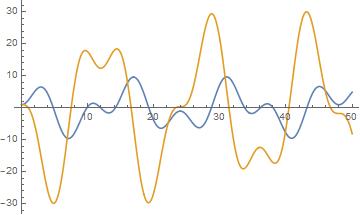
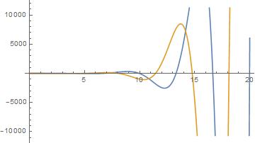
Figure 7: Motions around a Lagrange point are bounded for $\mu=0.02<1/27$ and unbounded for $\mu=0.4>1/27$.

The reader might have noticed that the equations (6.6) are mapped into our previous equations (3.8) by replacing the $-\lambda_{i}$ with $\Omega_{\pm}^{2}$. For the latter set of equations we found stability (trigonometric functions) provided that the frequency- squares are both positive, making seemingly unnecessary the stability condition (6.8). In sec.3 however we have worked with the specific condition $\frac{1}{2}\left(\Omega_{+}^{2}+\Omega_{-}^{2}\right)=1$, which does not apply here, so that the solutions (3.15) can not be used directly. Setting $c=\sqrt{1-3\mu(1-\mu)}$ and $\Delta=9c^{2}-8=1-27\mu(1-\mu)$, the chiral decomposition (3.10) has coefficients

$$\alpha_{\pm}=\frac{1}{4}(4-3c\mp\sqrt{\Delta}),\quad\beta_{\pm}=\frac{1}{4}(4+3c\mp\sqrt{\Delta}),$$ (6.9)

which are real when $\Delta\geq 0$, i.e., when $\mu(1-\mu)\leq\frac{1}{27}\,.$ Then the Hamiltonian $H$ and the symplectic $2-$form $\sigma$ are decomposed as

$$H=\frac{\sqrt{\Delta}}{16}\left[\big{(}\sqrt{\Delta}-4+3c\big{)}X^{2}_{+}X^{2}_{+}+\big{(}\sqrt{\Delta}-4-3c\big{)}X^{1}_{+}X^{1}_{+}\right.$$ (6.10a)

$$\qquad\left.+\big{(}\sqrt{\Delta}+4-3c\big{)}X^{2}_{-}X^{2}_{-}+\big{(}\sqrt{\Delta}+4+3c\big{)}X^{1}_{-}X^{1}_{-}\right],$$ (6.10b)

$$\sigma=\frac{\sqrt{\Delta}}{2}\left[dX^{1}_{+}\wedge dX^{2}_{+}-dX^{1}_{-}\wedge dX^{2}_{-}\right]\,,$$ (6.10c)

whose regularity requires $\Delta\neq 0$. In conclusion, the condition (6.8) should hold. Then the corresponding solutions,

$$\hat{\xi}=A\cos(\sqrt{\alpha_{+}\beta_{+}}\,t)+B\sin(\sqrt{\alpha_{+}\beta_{+}}\,t)$$

$$\hskip 17.07164pt+\,C\cos(\sqrt{\alpha_{-}\beta_{-}}\,t)+D\sin(\sqrt{\alpha_{-}\beta_{-}}\,t),$$ (6.11a)

$$\hat{\eta}=\sqrt{\frac{\beta_{+}}{\alpha_{+}}}\left(-A\sin(\sqrt{\alpha_{+}\beta_{+}}\,t)+B\cos(\sqrt{\alpha_{+}\beta_{+}}\,t)\right)$$

$$\hskip 17.07164pt+\,\sqrt{\frac{\beta_{-}}{\alpha_{-}}}\left(-C\sin(\sqrt{\alpha_{-}\beta_{-}}\,t)+D\cos(\sqrt{\alpha_{-}\beta_{-}}\,t)\right)$$ (6.11b)

are manifestly bounded, because $\Delta<1$ implies $\alpha_{\pm}\beta_{\pm}=\frac{1}{2}\left(1\mp\sqrt{\Delta}\right)>0.$

7 Conclusion

The striking similarities of the seemingly far remote topics discussed in this paper have, from the mathematical point of view, a simple explanation: in all cases, the problem boils down to study an anisotropic oscillator Alvarez ; ZGH ; ZHAGK . In the Paul [alias linearly polarized GW] case, the solution is expressed in terms of Mathieu functions PaulNobel ; Harte ; POLPER ; in the circularly polarized periodic GW case, they involve trigonometric/hyperbolic functions.

Previous investigations of the memory effect focused on sudden bursts of sandwich waves which vanish outside a short “wave zone”. It was advocated velmem that their observation would (theoretically) be possible due to the velocity memory effect : in the flat “afterzone” the particles move indeed with constant velocity, as required by …Newton’s 1st law ShortLong ; ImpMemory ; POLPER .

In this paper we study instead periodic waves sought for in inflationary models Bmode ; LIGOPer . Such waves have no “before and after-zone”, and their observation would require a different technique. Here we argue that, by analogy with ion trapping PaulNobel ; DehmeltNobel , one might study bound motions.

The Eisenhart lift of the 3D Paul trap is a linearly polarized periodic gravitational wave in 5D. For 3D Penning traps we find that, despite strong similarity with the equations which govern circularly polarized gravitational waves, their Eisenhart lift is not a CPP wave. However a slight modification (see sec. 5.3) allows for anisotropy and for a special value (5.18) of the frequencies we do get circularly polarized gravitational waves in 5D. Such perturbations were actually considered before as due to imperfections, see eqn. # (2.71) of ref. Brown .

It is remarkable that molecular physicist who worked on ion traps decades ago, were, like Molière’s Monsieur Jourdain, studying gravitational waves.

While our investigations here are classical, the chiral decomposition, (3.11b), makes it easy to study the quantum problem. Observing in particular the bound-state spectrum (5.23) could, theoretically, lead to the detection of such a wave. We mention that ion traps have also been studied recently in connection with (space)time crystals STcrystals .

It is worth to emphasize that these kinds of analogies extend very generally, even for non-periodic waves: the geodesic deviation equation in a vacuum background always looks like $\ddot{\xi}=R\xi$ in a parallel-propagated frame, where $R$ is an appropriate matrix. But this is an anisotropic oscillator equation and such equations are ubiquitous in physics. Moreover, time dependence in $R$ can give parametric resonance and similar things, as is well-known in other contexts. Geodesic motion in curved spacetimes is therefore generically linked to time-dependent anisotropic oscillators. Plane wave spacetimes are special here because i) it’s not awkward to let $R$ have any time dependence you like, and ii) the geodesic deviation equation is exact even for finite separations.

- (1) Ya. B. Zel’dovich and A. G. Polnarev, “Radiation of gravitational waves by a cluster of superdense stars,” Astron. Zh. 51, 30 (1974) [Sov. Astron. 18 17 (1974)].
- (2) V B Braginsky and L P Grishchuk, “Kinematic resonance and the memory effect in free mass gravitational antennas,” Zh. Eksp. Teor. Fiz. 89 744-750 (1985) [Sov. Phys. JETP 62, 427 (1985)].
- (3) M. Favata, “The gravitational-wave memory effect,” Class. Quant. Grav. 27 (2010) 084036 doi:10.1088/0264-9381/27/8/084036 [arXiv:1003.3486 [gr-qc]].
- (4) J. Podolský, C. Sämann, R. Steinbauer and R. Svarc, “The global existence, uniqueness and -regularity of geodesics in nonexpanding impulsive gravitational waves,” Class. Quant. Grav. 32 (2015) no.2, 025003 doi:10.1088/0264-9381/32/2/025003 [arXiv:1409.1782 [gr-qc]].
- (5) P.-M. Zhang, C. Duval, G. W. Gibbons and P. A. Horvathy, “The Memory Effect for Plane Gravitational Waves,” Phys. Lett. B 772 (2017) 743. doi:10.1016/j.physletb.2017.07.050 [arXiv:1704.05997 [gr-qc]]. “Soft gravitons and the memory effect for plane gravitational waves,” Phys. Rev. D 96 (2017) no.6, 064013 doi:10.1103/PhysRevD.96.064013. [arXiv:1705.01378 [gr-qc]].
- (6) A. I. Harte, “Optics in a nonlinear gravitational plane wave,” Class. Quant. Grav. 32 (2015) no.17, 175017 doi:10.1088/0264-9381/32/17/175017 [arXiv:1502.03658 [gr-qc]].
- (7) M. Faber and M. Suda, “Influence of gravitational waves on circular moving particles,” J. Mod. Phys. 9 (2018) no.4, 651 doi:10.4236/jmp.2018.94045 [arXiv:1704.07668 [gr-qc]].
- (8) G. M. Shore, “A New Twist on the Geometry of Gravitational Plane Waves,” JHEP 1709 (2017) 039 doi:10.1007/JHEP09(2017)039 [arXiv:1705.09533 [gr-qc]].
- (9) W. Kulczycki and E. Malec, “Axial gravitational waves in FLRW cosmology and memory effects,” Phys. Rev. D 96 (2017) no.6, 063523 doi:10.1103/PhysRevD.96.063523 [arXiv:1706.09620 [gr-qc]].
- (10) J. W. Maluf, J. F. Da Rocha-Neto, S. C. Ulhoa and F. L. Carneiro, “Plane Gravitational Waves, the Kinetic Energy of Free Particles and the Memory Effect,” Gravitation and Cosmology, Vol. 24, Issue 3 (2018) [arXiv:1707.06874 [gr-qc]].
- (11) P.-M. Zhang, C. Duval and P. A. Horvathy, “Memory Effect for Impulsive Gravitational Waves,” Class. Quant. Grav. 35 (2018) no.6, 065011 doi:10.1088/1361-6382/aaa987 [arXiv:1709.02299 [gr-qc]].
- (12) P. M. Zhang, C. Duval, G. W. Gibbons and P. A. Horvathy, “Velocity Memory Effect for Polarized Gravitational Waves,” JCAP 1805 (2018) no.05, 030 doi:10.1088/1475-7516/2018/05/030 [arXiv:1802.09061 [gr-qc]].
- (13) M. Kamionkowski, A. Kosowsky and A. Stebbins, “Statistics of cosmic microwave background polarization,” Phys. Rev. D 55 (1997) 7368 [astro-ph/9611125]. M. Kamionkowski and E. D. Kovetz, “The Quest for B Modes from Inflationary Gravitational Waves,” Ann. Rev. Astron. Astrophys. 54 (2016) 227 doi:10.1146/annurev-astro-081915-023433 [arXiv:1510.06042 [astro-ph.CO]].
- (14) B. P. Abbott et al. [LIGO Scientific and Virgo Collaborations], “All-sky Search for Periodic Gravitational Waves in the O1 LIGO Data,” Phys. Rev. D 96 (2017) no.6, 062002 doi:10.1103/PhysRevD.96.062002 [arXiv:1707.02667 [gr-qc]].
- (15) A. Ilderton, “Screw-symmetric gravitational waves: a double copy of the vortex,” Phys. Lett. B 782 (2018) 22 doi:10.1016/j.physletb.2018.04.069 [arXiv:1804.07290 [gr-qc]].
- (16) K. Andrzejewski and S. Prencel, “Memory effect, conformal symmetry and gravitational plane waves,” Phys. Lett. B 782 (2018) 421 doi:10.1016/j.physletb.2018.05.072 [arXiv:1804.10979 [gr-qc]].
- (17) E. Kilicarslan and B. Tekin, “Graviton Mass and Memory,” [arXiv:1805.02240 [gr-qc]].
- (18) W. Paul, “Electromagnetic Traps for charged and neutral particles.” Nobel Lecture (1989). Rev. Mod. Phys. 62 (1990) 531. doi:10.1103/RevModPhys.62.531
- (19) R. Blümel, C. Kappler, W. Quint, and J. Walter, “Chaos and order of laser-cooled ions in a Paul Trap ,” Phys. Rev. A40, 808 (1989). Erratum: Phys. Rev. A46, 80348 (1992).
- (20) H. G. Dehmelt, “Experiments with an isolated subatomic particle at rest,” Nobel Lecture (1989). Rev. Mod. Phys. 62 (1990) 525. doi:10.1103/RevModPhys.62.525
- (21) L. S. Brown and G. Gabrielse, “Geonium Theory: Physics of a Single Electron or Ion in a Penning Trap,” Rev. Mod. Phys. 58 (1986) 233. doi:10.1103/RevModPhys.58.233
- (22) K. Blaum, “High-accuracy mass spectrometry with stored ions,” Physics Reports 425 (2006) 1.
- (23) I. Białynicki-Birula, “Particle beams guided by electromagnetic vortices: New solutions of the Lorentz, Schrödinger, Klein-Gordon and Dirac equations,” Phys. Rev. Lett. 93 (2004) 020402 doi:10.1103/PhysRevLett.93.020402 [physics/0403078].
- (24) I. Białynicki-Birula, M. Kalinski and J. H. Eberly, “Lagrange Equilibrium Points in Celestial Mechanics and Nonspreading Wave Packets for Strongly Driven Rydberg Electrons,” Phys. Rev. Lett. 73 (1994) 1777. doi:10.1103/PhysRevLett.73.1777
- (25) Iwo Bialynicki-Birula, “Trojan Dynamics: From the Solar System to Molecules, Atoms, and Electrons,” (2006). http://www.cft.edu.pl/ birula/pliki/lectures/TrojanDynamics.pdf
- (26) C. Duval, G. Burdet, H. P. Künzle and M. Perrin, “Bargmann structures and Newton-Cartan theory”, Phys. Rev. D 31 (1985) 1841 ; C. Duval, G.W. Gibbons, P. Horvathy, “Celestial mechanics, conformal structures and gravitational waves,” Phys. Rev. D43 (1991) 3907. [hep-th/0512188].
- (27) M. W. Brinkmann, “Einstein spaces which are mapped conformally on each other,” Math. Ann. 94 (1925) 119–145.
- (28) P. Kosinski (private communication 2018, cited in POLPER .)
- (29) H. Bondi, F. A. E. Pirani and I. Robinson, “Gravitational waves in general relativity. 3. Exact plane waves,” Proc. Roy. Soc. Lond. A 251 (1959) 519. doi:10.1098/rspa.1959.0124
- (30) D. Kramer, H. Stephani, M. McCallum, E. Herlt, “Exact solutions of Einstein’s field equations,” Cambridge Univ. Press 2nd ed. (2003) sec 24.5 Table 24.2, p.385.
- (31) C. G. Torre, “Gravitational waves: Just plane symmetry,” Gen. Rel. Grav. 38 (2006) 653 [gr-qc/9907089].
- (32) R. Sippel and H. Goenner, “Symmetry classes of pp-waves,” Gen. Rel. Grav. 18, 1229 (1986).
- (33) J-M. Souriau, “Ondes et radiations gravitationnelles,” Colloques Internationaux du CNRS No 220, 243. Paris (1973).
- (34) C. Duval, G. W. Gibbons, P. A. Horvathy and P.-M. Zhang, “Carroll symmetry of plane gravitational waves,” Class. Quant. Grav. 34 (2017) 175003. doi.org/10.1088/1361-6382/aa7f62. [arXiv:1702.08284 [gr-qc]].
- (35) P. D. Alvarez, J. Gomis, K. Kamimura and M. S. Plyushchay, “Anisotropic harmonic oscillator, non-commutative Landau problem and exotic Newton-Hooke symmetry,” Phys. Lett. B 659 (2008) 906 doi:10.1016/j.physletb.2007.12.016 [arXiv:0711.2644 [hep-th]]; “(2+1)D Exotic Newton-Hooke Symmetry, Duality and Projective Phase,” Annals Phys. 322 (2007) 1556 doi:10.1016/j.aop.2007.03.002 [hep-th/0702014].
- (36) P. M. Zhang, G. W. Gibbons and P. A. Horvathy, “Kohn’s theorem and Newton-Hooke symmetry for Hill’s equations,” Phys. Rev. D 85 (2012) 045031 [arXiv:1112.4793 [hep-th]].
- (37) P. M. Zhang, P. A. Horvathy, K. Andrzejewski, J. Gonera and P. Kosinski, “Newton-Hooke type symmetry of anisotropic oscillators,” Ann. Phys. 333, 335 (2013). [arXiv:1207.2875 [hep-th]].
- (38) P. M. Zhang, M. Elbistan, G. W. Gibbons and P. A. Horvathy, “Sturm-Liouville and Carroll: at the heart of the Memory Effect,” Gen. Rel. Grav. 50 (2018) no.9, 107 doi:10.1007/s10714-018-2430-0 [arXiv:1803.09640 [gr-qc]].
- (39) C. Duval, P. A. Horváthy and L. Palla, “Conformal properties of Chern-Simons vortices in external fields,” Phys. Rev. D50, 6658 (1994). [hep-ph/9405229, hep-th/9404047].
- (40) M. Kretzschmar, “Particle motion in a Penning Trap”, Eur. J. Phys. 12 (1991) 240.
- (41) J. Danby, Fundamentals of celestial mechanics (Willman-Bell, Richmond, 1992).
- (42) V. B. Braginsky and K. S. Thorne, “Gravitational-wave bursts with memory experiments and experimental prospects”, Nature 327, 123 (1987). H. Bondi and F. A. E. Pirani, “Energy conversion by gravitational waves,” Nature 332 (1988) 212; “Gravitational Waves in General Relativity. 13: Caustic Property of Plane Waves,” Proc. Roy. Soc. Lond. A 421 (1989) 395. doi:10.1098/rspa.1989.0016 L. P. Grishchuk and A. G. Polnarev, “Gravitational wave pulses with ‘velocity coded memory’,” Sov. Phys. JETP 69 (1989) 653 [Zh. Eksp. Teor. Fiz. 96 (1989) 1153].
- (43) Tongcang Li, Zhe-Xuan Gong, Zhang-Qi Yin, H. T. Quan, Xiaobo Yin, Peng Zhang, L.-M. Duan, and Xiang Zhang, “Space-time crystals of trapped ions,” Phys. Rev. Lett. 109, 163001 (2012) doi. 10.1103/PhysRevLett.109.163001 [arXiv:1206.4772v2]
- (44) P.-M. Zhang, M. Cariglia, C. Duval, M. Elbistan, G. W. Gibbons, and P. A. Horvathy, “Erratum: Ion traps and the memory effect for periodic gravitational waves [Phys. Rev. D 98, 044037 (2018)]”, Phys. Rev. D 98, 089901(E) (2018).DOI: 10.1103/PhysRevD.98.089901