A-priori study of the subgrid energy transfers for small-scale dynamo in kinematic and saturation regimes

Abstract

The statistical properties of the subgrid energy transfers of homogeneous small-scale dynamo are investigated during the kinematic, nonlinear and statistically saturated stages. We carry out an a priori analysis of data obtained from an ensemble of direct numerical simulations on $512^{3}$ grid points and at unity magnetic Prandtl number. In order to provide guidance for subgrid-scale (SGS) modelling of different types of energy transfer that occur in magnetohydrodynamic dynamos, we consider the SGS stress tensors originating from inertial dynamics, Lorentz force and the magnetic induction separately. We find that all SGS energy transfers display some degree of intermittency as quantified by the scale-dependence of their respective probability density functions. Concerning the inertial dynamics, a depletion of intermittency occurs in presence of a saturated dynamo.

I Introduction

All turbulent flows are characterized by spatially and temporally chaotic evolutions on a wide range of scales and frequencies Frisch95 . As a result, direct numerical simulations (DNS) approaches are still not practical to study many turbulent flows occurring in nature and in engineering applications. The control parameter is given by the Reynolds number, $Re_{L}=UL/\nu$ a dimensionless measure of the relative importance of advective and viscous terms in the Navier-Stokes equations (NSE), where $U$ denotes the rms velocity fluctuations at the energy injection scale, $L$. It is possible to estimate that in homogeneous and isotropic turbulent flows the number of active degrees of freedom grows as $Re_{L}^{9/4}$ Landau59 , leading to extremely demanding numerical resources already for moderate turbulent intensities.
To overcome the problem, numerical tools based on a modeling of small-scale turbulent fluctuations are often introduced, and called large eddy simulations (LES). This technique is based on filtering out the small-scale interactions and replacing them with subgrid-scale (SGS) models Piomelli99 ; meneveau2000 ; pope2001 .
The demand for LES is increasing for magnetohydrodynamic (MHD) problems, too, as e.g. in heliophysical and astrophysical applications miesch2015 and in the context of liquid metal MHD. Furthermore, the LES technique is a useful alternative to spectral approaches in theoretical analyses of interscale energy transfer Aluie17 , in particular with a view towards applications in wall-bounded (i.e. liquid metal) flows. In MHD-LES, the small-scale nonlinear magnetic interactions and the velocity/magnetic correlations have to be replaced with SGS models, too. This introduces additional complexity to the MHD-LES method Kessar16 ; Aluie17 , leading to different modeling approaches Zhou91 ; Theobald94 ; Agullo01 ; Mueller02a ; muller2002 ; Knaepen04 ; haugen2006 ; Baerenzung08 ; Balarac10 ; Chernyshov10 . As in LES of nonconducting fluids, the success of a given model is usually assessed in terms of reproducing mean profiles of large scale quantities. However, it is more and more clear that SGS velocity fluctuations are characterized by extreme events with magnitudes comparable to that of the large-scale velocity root mean squares. Departure from Gaussian distribution becomes larger and larger by decreasing the scales where velocity and/or magnetic fluctuations are evaluated, a phenomenon known as intermittency Frisch95 ; Biskamp03 ; Verma04 . As a result, due to their statistical relevance and intensity, extreme events cannot be neglected when modeling SGS dynamics cerutti1998intermittency ; Buzzicotti18a . Intermittency and anomalous scaling have attracted the attention of several studies on MHD turbulence Politano95 ; Servidio09 ; Mininni09 ; Sahoo11 ; Yoshimatsu11 ; Imazio13 ; Meyrand15 ; Yang17 , with particular interest in high Reynolds number astrophysical applications, e.g. solar wind Veltri99 ; Salem09 ; Wan12 ; Matthaeus15 . The development of SGS models which are sophisticated enough to capture extreme events, and therefore provide a more faithful representation of turbulent dynamics, requires a detailed analysis of SGS quantities. A-priori studies of DNS data provide a first test-bed from where to extract the necessary information. The aim is to analyse the SGS correlations of the original fields and understand what the key features are that must be modeled. To our knowledge, there are very few a-priori studies for the MHD-LES formulation Balarac10 ; Kessar16 ; Grete16 Grete15 , all of which concerning statistically stationary nonlinear dynamos and without any focus on intermittency. The aim of this paper is to analyse the SGS properties of a MHD turbulent flow at different temporal instants during the evolution of a small-scale dynamo such as to be able to assess both regimes, when the magnetic field is passively advected by, or actively reacting on, the velocity field. In particular, we perform a systematic analysis of the different components of the SGS total energy transfer. We first split it in two sub-channels, involving velocity or magnetic temporal dynamics only and we analyse the mutual scale-by-scale energy exchanges. Second, we further decompose the kinetic SGS energy component into two contributions, one coming from the advection and one from the Lorentz force.
Furthermore, we also apply a formulation of the filtered fields, based on an exact projection on a finite number of Fourier modes (P-LES) Buzzicotti18a that disentangles the signal due to the coupling between resolved and unresolved scales from that due to interactions between resolved fields only.

The main results of this study are:
(i) The SGS energy transfer shows some degree of intermittency in all evolutionary stages of the dynamo. Its component coming from the Lorentz force becomes successively more intermittent while that originating from hydrodynamics shows decreased intermittency.
(ii) In terms of guidance for LES modelling, we find that dissipative models should be well suited for the SGS stresses connected with the Lorentz force, while not being suitable for those coming from purely inertial dynamics.

This paper is organized as follows: We begin in section II with a description of the DNS dataset. In section III, we introduce the P-LES formulation for MHD. Section IV presents the results from the a-priori analysis of the statistical properties of the SGS energy transfers. We summarize and discuss our results in section V.

II Description of the dataset

$M$	${\rm Re}_{L}$	${\rm Re}_{\lambda}$	$\varepsilon$	$U$	$L$	$\nu$	$T$	$k_{max}\eta_{u}$
512	889	164	0.14	0.61	1.0	0.0007	1.7	1.3

Table 1: Description of the statistically stationary hydrodynamic simulation used as an initial condition for the velocity fields in the dynamo runs. $M$ denotes the number of grid points in each Cartesian coordinate, ${\rm Re}_{L}$ the integral-scale Reynolds number, ${\rm Re}_{\lambda}$ the Reynolds number with respect to the Taylor microscale, $\varepsilon$ the total dissipation rate, $U$ the rms velocity, $L$ the integral length scale of the turbulence, $\nu$ the kinematic viscosity, $T=L/U$ the large-eddy turnover time, $k_{\rm max}$ the largest resolved wave number and $\eta_{u}$ the Kolmogorov microscale. All observables are time averaged.

The data for the a priori study is generated through DNSs of the three-dimensional incompressible MHD equations

$$\partial_{t}\bm{u}+\left(\bm{u}\cdot\nabla\right)\bm{u} =-\nabla p+\left(\nabla\times\bm{b}\right)\times\bm{b}+\nu\Delta\bm{u}+\bm{f},$$ (1)

$$\partial_{t}\bm{b} =\nabla\times\left(\bm{u}\times\bm{b}\right)+\eta\Delta\bm{b},$$ (2)

$$\nabla\cdot\bm{u} =0,\ \ \nabla\cdot\bm{b}=0,$$ (3)

where $\bm{u}$ is the velocity field, $\bm{b}$ the magnetic field in Alfvén units, $p$ the pressure divided by the density, $\nu$ the kinematic viscosity, $\eta$ the magnetic resistivity, and $\bm{f}$ an external mechanical force which is solenoidal at all times. The density has been set to unity for convenience.

Equations (1)-(3) are solved numerically on the periodic domain $V=[0,2\pi]^{3}$ using the pseudospectral method Orszag69 with full dealiasing by the $2/3$rds rule Orszag71 . An ensemble of 10 runs is generated, where the initial velocity field configurations are obtained from a statistically stationary hydrodynamic DNS on $512^{3}$ grid points by sampling in intervals of one large-eddy turnover time $T=L/U$, where $U$ is the rms velocity and $L$ the integral scale of the turbulence. The mechanical force $\bm{f}$ is a Gaussian-distributed and delta-in-time correlated random process acting at wavenumbers $1\leq k\leq 2.5$ with a flat spectrum and without injection of kinetic helicity. The magnetic seed fields are randomly generated with a Gaussian distribution and concentrated at wavenumber $k_{\rm s}=40$. Details of the stationary hydrodynamic simulation are summarized in table I.

	${\rm Re}_{L}$	${\rm Re}_{\lambda}$	$\rm Pm$	$\varepsilon_{u}$	$\varepsilon_{b}$	$U$	$L$	$B$	$L_{b}$	$\eta$	$k_{\rm max}\eta_{u}$	$k_{\rm max}\eta_{b}$	$t_{S}/T$
(I)	811	161	1	0.099	$2.6\cdot 10^{-3}$	0.59	0.97	0.020	0.092	0.0007	1.3	3.2	8.8
(II)	851	208	1	0.057	0.056	0.58	1.0	0.13	0.15	0.0007	1.5	1.5	17.6
(III)	870	211	1	0.032	0.076	0.51	1.2	0.25	0.29	0.0007	1.7	1.4	32.3

Table 2: Summary of the dynamo simulations during kinematic (I), nonlinear (II) and saturated stages (III). ${\rm Re}_{L}$ denotes the integral-scale Reynolds number, ${\rm Re}_{\lambda}$ the Reynolds number with respect to the Taylor microscale, $\rm Pm$ the magnetic Prandtl number, $\varepsilon_{u}$ the kinetic dissipation rate, $\varepsilon_{b}$ the magnetic dissipation rate, $U$ the rms velocity, $L$ the integral length scale of the turbulence, $B$ the rms of the magnetic field, $L_{b}$ the magnetic integral length scale, $\eta$ the resistivity, $k_{\rm max}$ the largest resolved wavenumber, $\eta_{u}$ and $\eta_{b}$ are the kinetic and magnetic Kolmogorov microscales, respectively, and $t_{S}$ is the sampling time of each evolutionary stage of the dynamo. All observables are ensemble-averaged over an ensemble of 10 simulations.

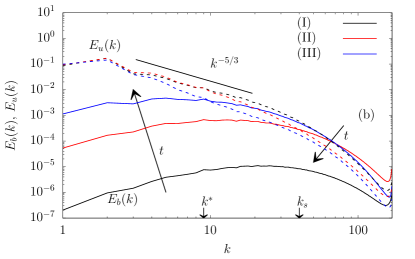
Figure 1: Panel (a): Time evolution of the kinetic energy $E_{u}$, the magnetic energy $E_{b}$ and the total energy $E_{u}+E_{b}$ with time measured in units of large-eddy turnover time $T$ (see table 1). The inset shows the evolution $E_{b}$ on a linear-logarithmic scale to highlight its initial exponential growth phase. The different stages of dynamo evolution are indicated by arrows: (I): kinematic stage, (II) nonlinear stage, (III) saturated stage. Panel (b): Kinetic energy spectra $E_{u}(k)$ (dashed) and magnetic energy spectra $E_{b}(k)$ (solid) measured at $t/T=8.8$ in stage (I), at $t/T=17.6$ in stage (II) and at $t/T=32.3$ in stage (III).

The time evolution of the kinetic and magnetic energies per unit volume

$$E_{u}(t) =\frac{1}{2}\left\langle|\bm{u}(\bm{x},t)|^{2}\right\rangle_{{V,N}}\equiv\left\langle\frac{1}{2|V|}\int d\bm{x}\ |\bm{u}(\bm{x},t)|^{2}\right\rangle_{{N}}\ ,$$ (4)

$$E_{b}(t) =\frac{1}{2}\left\langle|\bm{b}(\bm{x},t)|^{2}\right\rangle_{{V,N}}\equiv\left\langle\frac{1}{2|V|}\int d\bm{x}\ |\bm{b}(\bm{x},t)|^{2}\right\rangle_{{N}}\ ,$$ (5)

where the subscript $N$ denotes an ensemble average over $N=10$ realisations, and the total energy for the ensemble are shown in Fig. 1(a). From the time evolution of $E_{b}$, which is also shown on a linear-logarithmic scale in the inset, it can be seen that the simulation can be divided in three stages. First, during the kinematic stage (I), the magnetic field grows exponentially. During that stage the Lorentz force in Eq. (1) is negligible and the evolution equations are linear in the magnetic field. The exponential growth phase ends once the Lorentz force is large enough such that the back-reaction of the magnetic field on the flow needs to be taken into account. This is the nonlinear, unsteady, stage (II) of the evolution, during which $E_{b}$ continues to increase sub-exponentially Haugen04 ; Schekochihin04 . Finally, $E_{b}$ is approaching a statistically stationary state. That is, it enters the saturated stage (III) which at unity magnetic Prandtl number and sufficiently large ${\rm Re}$ is characterized by the ratios of the dissipation rates $\varepsilon_{b}/(\varepsilon_{u}+\varepsilon_{b})\simeq 0.7$ and energies $E_{b}/(E_{u}+E_{b})\simeq 0.25$ Haugen03 ; Brandenburg14 ; Linkmann17 ; McKay17 . Our data in stage (III) is consistent with these ratios, as can be seen from the values listed in table 2, where a summary of the dynamo runs in the kinematic (I), nonlinear (II) and saturated (III) stages is provided. The SGS energy transfers will be studied during stages (I)-(III), with each stage analysed separately.

The kinetic and the magnetic energy spectra

$$E_{u}(k,t) =\frac{1}{2}\left\langle\int_{|\bm{k}|=k}|\hat{\bm{u}}_{\bm{k}}(t)|^{2}\ d\bm{k}\right\rangle_{N}\ ,$$ (6)

$$E_{b}(k,t) =\frac{1}{2}\left\langle\int_{|\bm{k}|=k}|\hat{\bm{b}}_{\bm{k}}(t)|^{2}\ d\bm{k}\right\rangle_{N}\ ,$$ (7)

are shown in Fig. 1(b) for different instances in time corresponding to stages (I)-(III) as specified in table 2. The kinetic energy spectrum is dominated by the forcing in the interval $1\leq k\leq 2.5$. During the kinematic stage, an inertial subrange with Kolmogorov scaling can be identified, as indicated in the figure by the straight solid line. During stages (II) and (III) we observe a steepening of $E_{u}(k)$ at successively smaller wavenumbers. The magnetic energy spectrum grows self-similarly during stage (I) which is typical for a small-scale dynamo Schekochihin04 ; Mininni05a ; Brandenburg05 . In the saturated stage (III), the magnetic energy exceeds the kinetic energy at the small scales while the large scales remain essentially hydrodynamic and forcing-dominated. A crossover-wavenumber $k^{*}$ can be identified where $E_{u}(k^{*})=E_{b}(k^{*})$, in the present dataset $k^{*}=9$. Since the peak of the saturated magnetic energy spectrum depends on the forcing scale Brandenburg05 , the equipartition scale we measure will also not be universal, that is, it should depend on the forcing.

III P-LES formulation for MHD

The governing equations are derived by applying a filtering operation to the MHD equations Zhou91 ; Kessar16 ; Yang16a ; Aluie17 , with the filtered component $\overline{h}$ of a function $h$ defined as

$$\overline{h}(\bm{x},t)\equiv\int_{V}d\bm{y}\,G\left(\bm{x}-\bm{y}\right)h(\bm{y},t)=\sum\limits_{\bm{k}\in\mathbb{Z}^{3}}\hat{G}(\bm{k})\hat{h}(\bm{k},t)e^{i\bm{k}\bm{x}},$$ (8)

where $G$ is the filter function and $\hat{\cdot}$ denotes the Fourier transform. Applying this filtering operation to Eqs. (1) and (2), we obtain the filtered momentum and induction equations given here in tensor notation

$$\partial_{t}\overline{u}_{i} =-\partial_{j}\left(\overline{\overline{u}_{i}\overline{u}_{j}}-\overline{\overline{b}_{i}\overline{b}_{j}}+\tau_{ij}^{I}-\tau_{ij}^{M}+\overline{p}\delta_{ij}\right)+\nu\partial_{jj}\overline{u}_{i}+{\overline{f}_{i}},$$ (9)

$$\partial_{t}\overline{b}_{i} =-\partial_{j}\left(\overline{\overline{b}_{i}\overline{u}_{j}}-\overline{\overline{u}_{i}\overline{b}_{j}}+{{\color[rgb]{0,0,0}\tau_{ij}^{b}}}\right)+\eta\partial_{jj}\overline{b}_{i},$$ (10)

where a summation over repeated indices is implied, and with

$$\tau_{ij}^{I}= \ \overline{u_{i}u_{j}}-\overline{\overline{u}_{i}\overline{u}_{j}},$$ (11)

$$\tau_{ij}^{M}= \ \overline{b_{i}b_{j}}-\overline{\overline{b}_{i}\overline{b}_{j}},$$ (12)

$$\tau_{ij}^{b}= \ \overline{b_{i}u_{j}}-\overline{\overline{b}_{i}\overline{u}_{j}}-(\overline{u_{i}b_{j}}-\overline{\overline{u}_{i}\overline{b}_{j}}),$$ (13)

where $\tau_{ij}^{I}$ is the inertial SGS tensor, $\tau_{ij}^{M}$ the Maxwell SGS tensor, and $\tau_{ij}^{b}$ the SGS tensor originating from the electromotive force in Eq. (2). It consists of two SGS-stresses which are related to each other by transposition. They are associated with different dynamics, that is with advection, $(\bm{u}\cdot\nabla)\bm{b}$, in case of $\overline{b_{i}u_{j}}-\overline{\overline{b}_{i}\overline{u}_{j}}$ or dynamo action through magnetic field-line stretching, $(\bm{b}\cdot\nabla)\bm{u}$, in case of $\overline{u_{i}b_{j}}-\overline{\overline{u}_{i}\overline{b}_{j}}$. However, as they have a common physical origin, the electric field $\bm{E}=\bm{u}\times\bm{b}$, we do not consider them separately.

Equations (9)-(10) are obtained by using solenoidality of both fields, the linearity of the filtering operator and including the terms which can be written as a gradient into the pressure gradient. As usual, the equations are not closed in terms of the resolved fields only, due to the fact that the SGS stress tensors depend on the product of two unresolved fields. Equations  (9)-(10) differ from those usually given in the MHD literature on LES Zhou91 ; Kessar16 ; Aluie17 through the additional filtering of products of two resolved fields. In conjunction with a projector filter, the latter ensures that after introducing SGS models, Eqs. (9) and (10) can be evolved on a finite computational grid Sagaut06 ; Buzzicotti18a , which can seen by supposing that $G$ in Eq. (8) is a Galerkin projector on a finite number of Fourier modes Buzzicotti18a . In what follows, we consider $G$ to be a projector and Eqs. (9)-(13) are referred to as the P-LES formulation.

The P-LES formulation has the further advantage that, unlike in the usual LES formulation, the SGS energy transfers based on the P-SGS tensors defined in Eqs. (11)-(13) do not contain couplings between the resolved fields Buzzicotti18a . The latter is very important for the evaluation of backscatter in a priori analyses of SGS energy transfers, since residual couplings between the resolved fields can be wrongly interpreted as backscatter events. We will come back to this point in Secs. III.1 and IV.1.

Finally, we point out that care must be taken in a-posteriori studies of MHD LES concerning $\overline{p}$ since it contains the magnetic SGS pressure term, which is not closed in terms of the resolved magnetic field. As such, a closure of Eq. (12) would lead to two models for the magnetic pressure term: an explicit one coming from the choice of model and an implicit one from the solution of the Poisson equation. However, the magnetic pressure term does not affect the global energy transfers and is thus not of direct relevance to the present a-priori study.

III.1 The resolved-scale energy transfer

Neglecting viscous, Joule dissipation and forcing terms, the P-LES kinetic and magnetic energy evolution equations read

$$\partial_{t}\frac{1}{2}\overline{u}_{i}\overline{u}_{i}+\partial_{j}A^{u}_{j} =-\Pi^{u}+(\partial_{j}\overline{u}_{i})(\overline{\overline{u}_{i}\overline{u}_{j}})-(\partial_{j}\overline{u}_{i})(\overline{\overline{b}_{i}\overline{b}_{j}}),$$ (14)

$$\partial_{t}\frac{1}{2}\overline{b}_{i}\overline{b}_{i}+\partial_{j}A^{b}_{j} =-\Pi^{b}+(\partial_{j}\overline{b}_{i})(\overline{\overline{b}_{i}\overline{u}_{j}})-(\partial_{j}\overline{b}_{i})(\overline{\overline{u}_{i}\overline{b}_{j}}),$$ (15)

where $A_{j}^{u}=\overline{u}_{i}(\overline{\overline{u}_{i}\overline{u}_{j}}-\overline{\overline{b}_{i}\overline{b}_{j}}+\overline{p}\delta_{ij}+\tau_{ij}^{I}-\tau_{ij}^{M})$ and $A_{j}^{b}=\overline{b}_{i}(\overline{\overline{b}_{i}\overline{u}_{j}}-\overline{\overline{u}_{i}\overline{b}_{j}}+{{\color[rgb]{0,0,0}\tau_{ij}^{b}}})$ result in flux terms that redistribute the energies in space and vanish under spatial averaging: $\langle\partial_{j}A_{j}^{u}\rangle_{V}=\langle\partial_{j}A_{j}^{b}\rangle_{V}=0$ . The P-SGS energy transfers $\Pi^{u}$ and $\Pi^{b}$ are defined as

$$\Pi^{u} =\Pi^{I}-\Pi^{M}=(\partial_{j}\overline{u}_{i})\tau_{ij}^{I}-(\partial_{j}\overline{u}_{i})\tau_{ij}^{M},$$ (16)

$$\Pi^{b} ={{\color[rgb]{0,0,0}(\partial_{j}\overline{b}_{i})\tau_{ij}^{b}}},$$ (17)

where $\Pi^{I}=-(\partial_{j}\overline{u}_{i})\tau_{ij}^{I}$ is the inertial SGS energy transfer, $\Pi^{M}=-(\partial_{j}\overline{u}_{i})\tau_{ij}^{M}$ the Maxwell SGS energy transfer and $\Pi^{b}$ the SGS energy transfer associated with the electromotive force. Equations (14) and (15) contain four extra terms: $(\partial_{j}\overline{u}_{i})(\overline{\overline{u}_{i}\overline{u}_{j}})$, $(\partial_{j}\overline{u}_{i})(\overline{\overline{b}_{i}\overline{b}_{j}})$, $(\partial_{j}\overline{b}_{i})(\overline{\overline{b}_{i}\overline{u}_{j}})$ and $(\partial_{j}\overline{b}_{i})(\overline{\overline{u}_{i}\overline{b}_{j}})$. Using $\nabla\cdot\overline{\bm{u}}=0$, $\nabla\cdot\overline{\bm{b}}=0$ and the projector property $\hat{G}^{2}=\hat{G}$, it can be shown that

$$\left\langle(\partial_{j}\overline{u}_{i})(\overline{\overline{u}_{i}\overline{u}_{j}})\right\rangle_{V}=0\ ,$$ (18)

$$\left\langle(\partial_{j}\overline{b}_{i})(\overline{\overline{b}_{i}\overline{u}_{j}})\right\rangle_{V}=0\ ,$$ (19)

and

$$\left\langle(\partial_{j}\overline{u}_{i})(\overline{\overline{b}_{i}\overline{b}_{j}})\right\rangle_{V}=-\left\langle(\partial_{j}\overline{b}_{i})(\overline{\overline{u}_{i}\overline{b}_{j}})\right\rangle_{V}\ ,$$ (20)

hence they do not contribute to the global total energy balance. Furthermore, it is easy to verify that out of the four terms only $(\partial_{j}\overline{u}_{i})(\overline{\overline{b}_{i}\overline{b}_{j}})$ is Galilean invariant. Galilean invariance is important to prevent the occurrence of unphysical fluctuations in the measured SGS energy transfer aluie2009I ; aluie2009II ; Buzzicotti18a . This problem can be solved by adding and subtracting energy transfers originating from the Leonard stress components for each SGS tensor leonard1975 ; Zhou91 in Eqs. (14) and (15). The Leonard stresses are defined as

$$\tau_{ij}^{I,L} =\overline{\overline{u}_{i}\overline{u}_{j}}-\overline{u}_{i}\overline{u}_{j},$$ (21)

$$\tau_{ij}^{M,L} =\overline{\overline{b}_{i}\overline{b}_{j}}-\overline{b}_{i}\overline{b}_{j},$$ (22)

$$\tau_{ij}^{b,L} ={{\color[rgb]{0,0,0}\overline{\overline{b}_{i}\overline{u}_{j}}-\overline{b}_{i}\overline{u}_{j}-(\overline{\overline{u}_{i}\overline{b}_{j}}-\overline{u}_{i}\overline{b}_{j})}},$$ (23)

which give rise to the following energy transfer terms

$$\Pi^{u,L} =\Pi^{I,L}-\Pi^{M,L}=(\partial_{j}\overline{u}_{i})\tau_{ij}^{I,L}-(\partial_{j}\overline{u}_{i})\tau_{ij}^{M,L},$$ (24)

$$\Pi^{b,L} ={{\color[rgb]{0,0,0}(\partial_{j}\overline{b}_{i})\tau_{ij}^{b,L}}}.$$ (25)

Including the Leonard terms in Eqs. (14) and (15) results in

$$\partial_{t}\frac{1}{2}\left(\overline{u}_{j}\overline{u}_{j}\right) +\partial_{j}\left(A^{u}_{j}+\overline{u}_{i}\tau_{ij}^{u,L}\right)$$

$$=-\Pi^{u}-\Pi^{u,L}-(\partial_{j}\overline{u}_{i})(\overline{b}_{i}\overline{b}_{j}),$$ (26)

$$\partial_{t}\frac{1}{2}\left(\overline{b}_{j}\overline{b}_{j}\right) +\partial_{j}\left(A^{b}_{j}+\overline{u}_{i}\tau_{ij}^{b,L}\right)$$

$$=-\Pi^{b}-\Pi^{b,L}+(\partial_{j}\overline{u}_{i})(\overline{b}_{i}\overline{b}_{j}).$$ (27)

Now all terms in the resolved energy evolution equations are Galilean invariant.

It is important to remark that the Leonard SGS transfers vanish under spatial averaging, i.e. they do not alter the global balances. Furthermore, they couple only the resolved fields, hence they cannot be associated with transfers between resolved and SGS quantities. Therefore the LES formulation differs from the P-LES formulation in a fundamental way: All SGS-tensors in the LES formulation are the sum of the respective P-SGS and Leonard tensors, e. g. $\tau_{ij}^{I,\rm LES}=\tau_{ij}^{I}+\tau_{ij}^{I,L}$, and the corresponding SGS energy transfers of the LES formulation contain the contribution from the Leonard stresses. That is, the SGS energy transfers in the LES formulation have contributions from interactions between the resolved fields Buzzicotti18a . We will come back to this point in the context of backscatter in Sec. IV.1 and in the Appendix.

Finally, the term $(\partial_{j}\overline{u}_{i})(\overline{b}_{i}\overline{b}_{j})$ occurs in Eqs. (III.1) and (III.1) with opposite sign. Since it is closed in terms of the resolved fields and exchanges kinetic and magnetic energy, $(\partial_{j}\overline{u}_{i})(\overline{b}_{i}\overline{b}_{j})$ has been named resolved-scale conversion term Aluie17 . It is positive if kinetic energy is converted to magnetic energy and negative vice versa. With $\Pi^{u}=\Pi^{I}-\Pi^{M}$ and $\Pi^{b}$ we now have key benchmark quantities to study the properties of the different SGS energy transfers. Furthermore, as the total energy is conserved in the absence of forcing and dissipation, the total SGS energy transfer is also a quantity of interest. We define the resolved total energy transfer $\Pi$ through the resolved-scale total energy balance

$$\partial_{t}\frac{1}{2}\left(\overline{u}_{i}\overline{u}_{i}\right)+\partial_{t}\frac{1}{2}\left(\overline{b}_{i}\overline{b}_{i}\right) +\partial_{j}\left(A_{j}+\overline{u}_{i}\tau_{ij}^{L}\right)$$

$$=-\Pi-\Pi^{L}$$ (28)

where $A_{j}=A^{u}_{j}+A^{b}_{j}$, $\tau_{ij}^{L}=\tau_{ij}^{u,L}+\tau_{ij}^{b,L}$, $\Pi=\Pi^{u}+\Pi^{b}$ and $\Pi^{L}=\Pi^{u,L}+\Pi^{b,L}$. Figure 2 gives a schematic overview of the different SGS energy transfers.

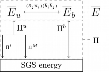
Figure 2: A schematic representation of the energy transfer between the resolved-scale energies and the SGS energy. The exchange between magnetic and kinetic energies at the resolved scales is carried by the resolved-scale conversion term $(\partial_{j}\overline{u}_{i})\overline{b}_{i}\overline{b}_{j}$. According to Eqs. (III.1) and (III.1), the exchange of energy between resolved scales and SGS follows different channels, $\Pi^{b}$ couples the resolved-scale magnetic energy to the SGS and combines the physical processes of advection of magnetic energy and magnetic field line stretching, while $\Pi^{u}$ transfers kinetic energy between resolved scales and SGS. The latter itself has two components, an inertial channel $\Pi^{I}$ which is due to vortex-stretching and advection and a magnetic channel $\Pi^{M}$ originating from the Lorentz force. During the kinematic stage of the dynamo, $\Pi^{M}$ is negligible compared to $\Pi^{I}$.

IV A priori analysis of the SGS energy transfers

The a priori analysis of the statistical properties of the SGS energy transfers is carried out using a sharp spectral cut-off filter, which is defined through its action on a generic function $h$

$$\overline{h}(\bm{x},t)\equiv\sum\limits_{|\bm{k}|<k_{c}}\hat{h}(\bm{k},t)e^{i\bm{k}\bm{x}},$$ (29)

where $k_{c}$ is the cut-off wavenumber, which corresponds to the configuration-space filter width $\Delta=\pi/k_{c}$. Although sharp projectors produce Gibbs oscillations in configuration space ray2011resonance resulting in SGS stress tensors vreman1994realizability that are not positive-definite, they have the advantage to create a clear distinction between resolved and unresolved scales and to allow all terms in the equations (9)-(10) to evolve on the same Fourier subspace for all times. Moreover, for nonconducting flows, a good agreement between the statistics of the SGS energy transfer obtained from a sharp cutoff and Gaussian filter was found Buzzicotti18a , suggesting that effects specific to Galerkin projection have only a subleading effect at the level of the energy evolution equations.

In what follows, we study the mean (here, mean refers to the combined spatial and ensemble average) P-SGS energy transfers and their spatial fluctuations for different $k_{c}$. The fluctuations are investigated through the probability density functions (pdfs) of the respective P-SGS energy transfers. In order to quantify the departure from Gaussianity at different scales, it is customary to evaluate the flatness $F_{x}$ of the standardized pdfs,

$$F_{x}(k_{c})=\langle x^{4}\rangle/\langle x^{2}\rangle^{2}\sim k_{c}^{\zeta},$$

as a function of the cutoff wavenumber, where $x$ represents the different contributions of the P-SGS energy transfer. Since the Leonard stresses do not provide information relevant to modelling, we summarize results specific to the Leonard stresses in the Appendix, which is referenced in the text where necessary.

We begin with $\Pi$, and subsequently increase the level of detail by first splitting $\Pi$ into $\Pi^{u}$ and $\Pi^{b}$, followed by the decomposition of $\Pi^{u}$ into $\Pi^{I}$ and $\Pi^{M}$. Note that $\Pi^{b}$ is not decomposed any further, because the stress tensors associated with the advection and field-line stretching terms in the induction equation originate both from the electric field and are related to each other by transposition, as discussed in Sec. III. As such, a single LES model term should be used in the induction equation.

IV.1 The total SGS energy transfer

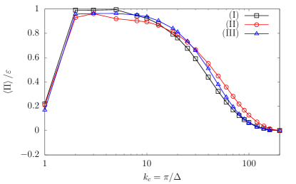
Figure 3: The mean total SGS energy transfer $\langle\Pi\rangle_{V,N}$ normalized with the total dissipation $\varepsilon$ versus the cutoff wavenumber $k_{c}$ at the kinematic (I), nonlinear (II) and stationary (III) stages.

Figure 3 presents $\left\langle\Pi\right\rangle_{V,N}$ as function of $k_{c}$ at three different instants during the time evolution which are representative of the three stages (I)-(III). Since $\Pi$ is obtained using a spectral cut-off projector, its mean value equals the total energy flux in Fourier space across the cut-off wavenumber $k_{c}=\pi/\Delta$, see eyink2005locality ; Buzzicotti18a . As can be seen from Fig. 3, $\left\langle\Pi\right\rangle_{V,N}\geqslant 0$, which is representative of a mean total energy transfer from large scales to small scales. Furthermore, we find that $\left\langle\Pi\right\rangle_{V,N}$ does not change significantly during the different evolutionary stages of the dynamo, which implies that the exchange of kinetic and magnetic energy proceeds in a way that leaves the total scale-by-scale transfer unaffected. We will come back to this point in further detail when assessing the decomposed SGS energy transfers.

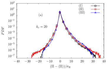
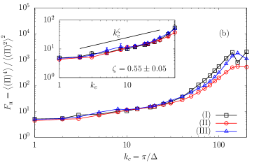
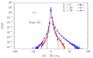
Figure 4: Total SGS energy transfer $\Pi$ during the kinematic stage (I), non-linear stage (II) and the stationary stage (III). Panel (a): pdfs of $\Pi$ at $k_{c}=20$. Panel (b): The flatness of $\Pi$ versus the cutoff wavenumber $k_{c}$. The inset shows a zoom of the flatness in the inertial range of scales, with error bars estimated from the different configurations. The black line represents the fit of the flatness scaling exponent in the range $2\leqslant k_{c}\leqslant 30$. Panel (c): pdfs of $\Pi$ at $k_{c}=8$, $k_{c}=20$ and $k_{c}=70$ during stage (II).

Since $\left\langle\Pi\right\rangle_{V,N}\geqslant 0$, it can be expected that the pdf of $\Pi$ is positively skewed such that events leading to a forward transfer of total energy across the filter scale are more likely than backscatter events. This is indeed the case as shown by the standardized pdf of $\Pi$ in Fig. 4(a) at $k_{c}=20$ for stages (I)-(III). Apart from more pronounced tails occurring in stage (II), the standardized pdfs are remarkably similar. However, while the pdf of $\Pi$ is positive skewed at all stages, the pdf of $\Pi^{L}$ is symmetric (see Fig. 12 in Appendix ). Hence, by measuring $\Pi=\Pi+\Pi^{L}$ as the total SGS energy transfer, the residual transfer amongst the resolved scales carried by the Leonard component could lead to the conclusion of backscatter events being more frequent than they actually are.

In Fig.4(b) we show the flatness of $\Pi$, ($F_{{}_{\Pi}}$), as a function of the cut-off wavenumber $k_{c}$. From this analysis we can see that the flatness shows a similar power-law behavior in the inertial range $2\leq k_{c}\leq 30$ during all stages in the evolution. The flatness scaling exponent $\zeta=0.55\pm 0.05,$ see inset of Fig. 4(b), has been measured by a least-squares fit and its error has been estimated by varying the fitting interval within the inertial range $2\leq k_{c}\leq 30$. A small temporal variability of the flatness is observed only in the dissipative range where it is also found to increase exponentially suggesting strong deviation from Gaussianity at all times. From both the pdfs and flatness analysis it follows that the statistical properties of $\Pi$ are conserved during the temporal evolution. Fig. 4(c) presents the pdfs of $\Pi$ at a fixed time during the non-linear stage (II) at three different cut-off wavenumbers $k_{c}=8$, $k_{c}=20$ and $k_{c}=70$. As can be seen from Figs. 1(b) and (3), $k_{c}=8$ and $k_{c}=20$ correspond to the beginning and the end of the inertial range, respectively, while $k_{c}=70$ lies in the dissipative range. From the comparison of the three standardized pdfs in Fig.4(c) we can clearly observe the presence of intermittency in the statistics of $\Pi$ through an increasing departure from Gaussianity at successively smaller scales. The same information can be extracted by the power-law behavior of the flatness over the inertial range of scales which also shows the intermittent properties of the SGS energy transfer in MHD turbulence. It is interesting to note that the value of $\zeta$ measured from the data is in agreement with the prediction of the She-Leveque model she1994universal . Indeed, from the scaling estimate,

$$\langle|\Pi|^{n}\rangle=O\left(\Delta^{\zeta_{3n}-n}\right),$$

eyink1996multifractal ; Buzzicotti18a and from the She-Leveque values of the exponents for n=2: $\zeta_{6}\sim 1.77$ and n=4: $\zeta_{12}\sim 1.94$ (note that there is a typo in the value of $\zeta_{12}$ reported in ref. Buzzicotti18a ), we obtain for the flatness the She-Leveque prediction $\zeta_{{}_{SL}}\sim 0.6$.

IV.2 Kinetic and magnetic SGS energy transfers

As discussed in Sec. III, $\Pi$ can be further decomposed into $\Pi^{u}$ and $\Pi^{b}$. Furthermore, the resolved-scale conversion term, $(\partial_{j}\overline{u}_{i})\overline{b}_{i}\overline{b}_{j}$, in Eqs. (III.1) and (III.1), which cancels out in Eq. (28) for the total resolved-scale energy, must also be measured. It contains information on the scale-dependence of the conversion of kinetic to magnetic energy, an assessment of which is essential in order to provide guidance for SGS models of MHD dynamos.
The averages $\left\langle\Pi^{u}\right\rangle_{V,N}$, $\left\langle\Pi^{b}\right\rangle_{V,N}$ and $\langle(\partial_{j}\overline{u}_{i})\overline{b}_{i}\overline{b}_{j}\rangle_{V,N}$ are shown in Fig. 5(a-c), respectively. We first notice that $\left\langle\Pi^{u}\right\rangle_{V,N}$ gets depleted towards stage (III) while $\left\langle\Pi^{b}\right\rangle_{V,N}$ increases. From a comparison of the large increase of $\langle(\partial_{j}\overline{u}_{i})\overline{b}_{i}\overline{b}_{j}\rangle_{V,N}$ relative to the smaller decrease of $\left\langle\Pi^{u}\right\rangle_{V,N}$ during stages (I)-(III), it follows that the growth of the magnetic field is due to direct interactions between $\overline{\bm{u}}$ and $\overline{\bm{b}}$. The data presented in Fig. 5(a,b) also show that both the kinetic and magnetic SGS energy transfers are forward. From Fig. 5(c) it can be seen that $\langle(\partial_{j}\overline{u}_{i})\overline{b}_{i}\overline{b}_{j}\rangle_{V,N}$ has an inflection point that saturates at $k^{*}\approx 20$. Since the large-scale conversion term is the running integral in $k$ of the energy transfer at $k$, an inflection point in $\langle(\partial_{j}\overline{u}_{i})\overline{b}_{i}\overline{b}_{j}\rangle_{V,N}$ at $k^{*}$ implies an extremum in the energy conversion at $k^{*}$, corresponding to a saturation length scale for the conversion of kinetic to magnetic energy. The existence of a saturation length scale implies the breaking of inertial self-similarity and puts a natural constraint on any LES for MHD. Either we use an extremely resolved model with $k_{c}\gg k^{*}$, and we fully resolve the dynamics leading to the non-linear dynamo saturation, or we use $k_{c}\sim k^{*}$ and a very sophisticated SGS model must be used. Certainly one cannot further push and use $k_{c}\ll k^{*}$, or a fully ad-hoc magnetic field growth must be supplied. An in-depth investigation of the statistical properties of the resolved-scale conversion term would provide guidance for cases where very coarse grids require the aforementioned ad-hoc magnetic forcing term. A quantitative assessment of this issue also requires a posteriori analyses and would constitute a useful contribution to MHD LES.

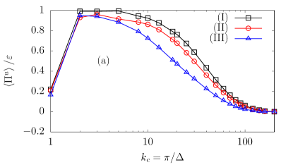
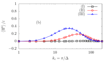
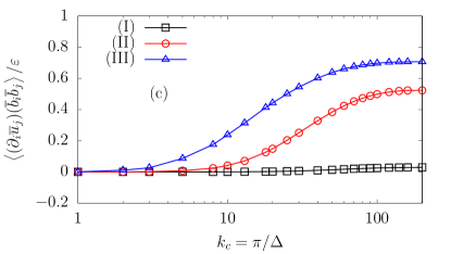
Figure 5: The mean P-SGS energy transfers $\langle\Pi^{u}\rangle_{V,N}$ (panel (a)), and $\langle\Pi^{b}\rangle_{V,N}$ (panel (b)), and the mean of resolved-scale conversion term $\langle(\partial_{j}\overline{u_{i}})\overline{b}_{i}\overline{b}_{j}\rangle_{V,N}$ (panel (c)), normalized with the total energy dissipation rate $\varepsilon$ versus the cutoff wavenumber $k_{c}$ during the kinematic (I), non-linear (II) and stationary (III) stages.

Figure 6(a,b) presents the standardized pdfs of $\Pi^{u}$ and $\Pi^{b}$ at $k_{c}=20$. We note that the pdfs of $\Pi^{b}$ are only shown for stages (II) and (III), as $\Pi^{b}$ is negligible in stage (I), because the system is dominated by magnetic field amplification which occurs through the term $(\partial_{j}\overline{u_{i}})\overline{b}_{i}\overline{b}_{j}$. Although $\langle\Pi^{u}\rangle_{V,N}$ and $\langle\Pi^{b}\rangle_{V,N}$ are positive, that is, kinetic and magnetic energies are transferred downscale on average, the pdfs of $\Pi^{u}$ and $\Pi^{b}$ develop negative tails. The latter is particularly pronounced for $\Pi^{b}$ in stage (III), as shown in Fig. 6(b). That is backscatter events in the magnetic SGS energy transfer cannot be neglected for a fully nonlinear dynamo. The latter implies that dissipative approaches such as the Smagorinsky closure Smagorinsky63 are hardly optimal to model the SGS stresses in the induction equation. The flatness of $\Pi^{u}$ and $\Pi^{b}$ as a function of $k_{c}$ is shown Figs. 6(c,d). There appears to be a slight indication of increased intermittency in stage (III) compared to stages (I) and (II) for both $\Pi^{u}$ and $\Pi^{b}$ since the flatness becomes more scale-dependent in the inertial range. As can be seen from the figures, $\Pi^{b}$ appears to be less intermittent than $\Pi^{u}$. However, the latter statements on intermittency require further assessment using higher-resolved datasets with a more extended inertial range.

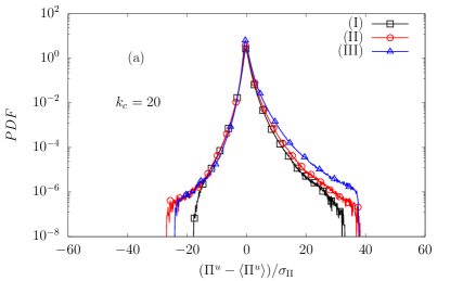
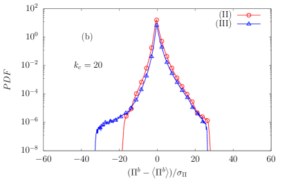
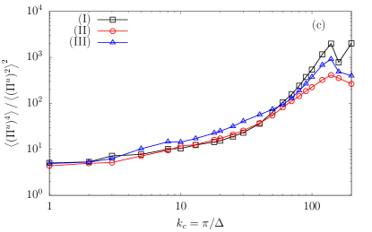
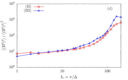
Figure 6: Kinetic and magnetic SGS energy transfers $\Pi^{u}$ and $\Pi^{b}$ during the kinematic stage (I), non-linear stage (II) and the stationary stage (III): pdfs of $\Pi^{u}$ (a) and $\Pi^{b}$ (b) at $k_{c}=20$; flatness of $\Pi^{u}$ (c) and $\Pi^{b}$ (d) against the cutoff wavenumber $k_{c}$.

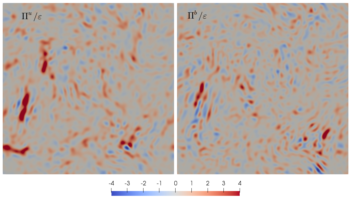
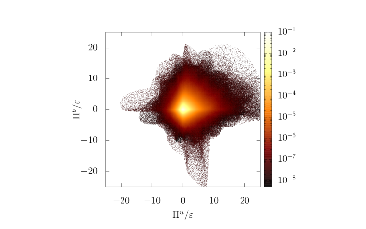
Figure 7: (Colour online) Top: Two-dimensional visualisations of $\Pi^{u}$ (left) and $\Pi^{b}$ (right) at $k_{c}=20$ in stage (III). Positive values correspond to forward energy transfer while negative values indicate backscatter. Bottom: Corresponding joint pdf of $\Pi^{u}$ and $\Pi^{b}$.

Visualisations of $\Pi^{u}$ and $\Pi^{b}$ obtained during stage (III) are presented in the top panels of Fig. 7. A striking feature is the localized elongated nature of intense forward-transfer events in $\Pi^{u}$. Similar structures are are also visible in $\Pi^{b}$ , and the colour-mapping suggests an inverse relation between $\Pi^{u}$ and $\Pi^{b}$, where large values of $\Pi^{u}$ are correlated with small values of $\Pi^{b}$ and vice versa. The correlation between $\Pi^{u}$ and $\Pi^{b}$ is quantified through their joint pdf shown in the bottom panel of Fig. 7. The data in the figure show a tendency towards higher probabilities along the axes where either $\Pi^{u}=0$ or $\Pi^{b}=0$, which suggest a mild inverse proportionality between the two. As will be seen later, the intense forward-transfer events in $\Pi^{u}$ originate from the P-SGS Maxwell stresses in Eq. (9).

IV.3 Inertial and Maxwell SGS energy transfers

The term $\Pi^{u}$ in Eq. (9) is now further decomposed into $\Pi^{I}$ and $\Pi^{M}$, as introduced in Sec. III. Figure 8 presents $\left\langle\Pi^{I}\right\rangle_{V,N}$ and $\left\langle-\Pi^{M}\right\rangle_{V,N}$ as functions of $k_{c}$ where the sign convention for $\Pi^{M}$ reflects the sign with which it occurs in Eq. (9). During the kinematic stage (I), $\left\langle\Pi^{M}\right\rangle_{V,N}$ is negligible and the total SGS energy transfer is carried by $\left\langle\Pi^{I}\right\rangle_{V,N}$. As expected $\langle\Pi^{I}\rangle_{V,N}$ gets depleted towards stage (III) while $\langle-\Pi^{M}\rangle_{V,N}$ increases. Both $\left\langle\Pi^{I}\right\rangle_{V,N}$ and $\left\langle-\Pi^{M}\right\rangle_{V,N}$ are positive, that is, the resolved-scale kinetic energy is transferred from large to small scales through inertial transfer as well as through the Maxwell component.

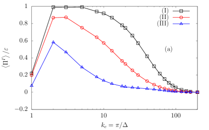
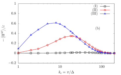
Figure 8: The mean components $\left\langle\Pi^{I}\right\rangle_{V,N}$ (a) and $\left\langle\Pi^{M}\right\rangle_{V,N}$ (b) versus the cutoff wavenumber $k_{c}$ at the kinematic stage (I), non-linear stage (II) and the stationary stage (III).

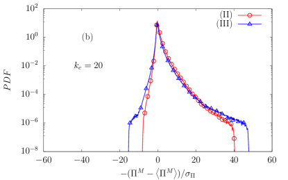
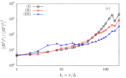
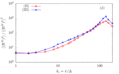
Figure 9: Fluctuations of $\Pi^{I}$ and $\Pi^{M}$ during kinematic (I), non-linear (II) and stationary (III) stages: pdfs of $\Pi^{I}$ (a) and $\Pi^{M}$ (b) at $k_{c}=20$; flatness of $\Pi^{I}$ (c) and $\Pi^{M}$ (d) against the cutoff wavenumber $k_{c}$.

Figures 9 (a,b) show the standardized pdfs of $\Pi^{I}$ and $\Pi^{M}$, respectively, where we note that the pdf of $\Pi^{M}$ is only shown in stages (II) and (III) as it is negligible in stage (I). During stages (II) and (III) the pdf of $\Pi^{I}$ changes significantly compared to its shape during stage (I), where the inertial dynamics are approximately unaffected by the magnetic field. The most striking feature here is the development of wide tails and a much more symmetric shape. That is, the inertial SGS energy transfer fluctuates very differently in presence of a fluctuating magnetic field as in the nonconducting case: First, the wide tails indicate that extreme events are more likely than in the nonconducting case. Second, the symmetric shape implies that backscatter events in the inertial SGS energy transfer become significant. In contrast, as can be seen from Fig. 9 (b), the pdf of $\Pi^{M}$ has a clear positive skewness. That is, backscatter events are much less important than for all other SGS energy transfer components and the contributions from the SGS Maxwell stresses should be well approximated by a dissipative model.

Measurements of the pdfs of ${\Pi^{I}+\Pi^{I,L}}$ and $\Pi^{M}+\Pi^{M,L}$ during the saturated stage of a small-scale dynamo have been reported recently Kessar16 . By comparison of Figs. 9 (a,b) with the left panel of Fig. 7 in Ref. Kessar16 , one observes that the shape of the pdfs measured in Ref. Kessar16 is quite different from the results found here for $\Pi^{I}$ and $\Pi^{M}$ . More precisely, the pdf of $\Pi^{I}+\Pi^{I,L}$ in Ref. Kessar16 lacks the wide tails seen for $\Pi^{I}$ here, and the pdf of $\Pi^{M}+\Pi^{M,L}$ is much more symmetric than that presented for $\Pi^{M}$ in Fig. 9(b). There are two reasons for latter difference. First, the Leonard component is included in the measurement of the SGS energy transfer in Ref. Kessar16 while it is not included here. Second, the Reynolds numbers and filter widths also differ. In Ref. Kessar16 the the pdfs were measured at ${\rm Re}_{\lambda}=75$ at a filter scale coresponding to $k_{c}=64$. For comparison, in our dataset ${\rm Re}_{\lambda}=211$, and the pdfs in Figs. 9 (a,b) are measured at $k_{c}=20$. Even in our simulations, it can be seen from the energy spectra (Fig. 1(b)) and the mean SGS energy transfer (Fig. 3) that the dynamics at $k_{c}=64$ is significantly affected by viscous and Joule dissipation. This will be even more so for lower ${\rm Re}_{\lambda}$. In order to provide a like-for-like comparison, we measured of the pdfs of $\Pi^{M}$, $\Pi^{M,L}$ and $\Pi^{M}+\Pi^{M,L}$ for $k_{c}=80$, which for our data at ${\rm Re}_{\lambda}=211$ is comparable to $k_{c}=64$ for ${\rm Re}_{\lambda}=75$. As can be seen in Fig. 13 in the Appendix, the pdf of $\Pi^{M,L}$ in the viscous range is sizeable and symmetric, such that the inclusion of $\Pi^{M,L}$ in the measurement of the Maxwell SGS transfer masks the distinctive positive skewness of its PDF.

Figures 9(c,d) present the flatness of $\Pi^{I}$ and $\Pi^{M}$ as functions of $k_{c}$. For $\Pi^{I}$, the development of strongly non-Gaussian statistics is also reflected in the flatness, which has higher values in stage (III) compared to stages (I) and (II). Furthermore, the flatness has a much weaker scale-dependence during stage (III) as shown in Fig. 9(c). This indicates a depletion of intermittency of the velocity field in presence of a saturated dynamo. Indeed, a comparison of the $p^{\rm th}$-order scaling exponents $\zeta_{p}$ of the velocity-field structure functions for hydrodynamic turbulence Gotoh02 and for a saturated MHD dynamo Haugen04 reveals differences in $\zeta_{p}$ for $p\geqslant 5$. According to these results, the velocity field is less intermittent in presence of a saturated dynamo, as observed here. Since $(\Pi^{I})^{p}$ is related to the $3p^{\rm th}$-order velocity-field structure function eyink2 the scaling properties of high-order structure functions determine the behavior of the flatness of $\Pi^{I}$. Therefore differences concerning intermittency between MHD and hydrodynamic turbulence are more clearly visible in measurements of the flatness of $\Pi^{I}$ compared to direct measurements of $\zeta_{p}$. However, a quantitative assessment of the scaling properties of the flatness of $\Pi^{I}$ requires a further extended scaling range. In contrast to the results for $\Pi^{I}$, the flatness of $\Pi^{M}$ shown in Fig. 9(d) retains its scale-dependence after dynamo saturation. As can be seen from the figure, the flatness of $\Pi^{M}$ has a much stronger scale dependence compared to $\Pi$. The stronger intermittent signal in $\Pi^{M}$ may be related to the fact that the saturated magnetic field is much more intermittent than the velocity field that maintains it, as shown by measurements of scaling exponents of inertial and magnetic structure functions obtained from DNSs of stationary small-scale dynamos Haugen04 . As in the present data, no mean magnetic field was present in the data analysed in Ref. Haugen04 .

As shown in Fig. 8(a), the mean inertial interscale energy transfer is weakened in presence of a saturated dynamo. This partly occurs through cancellations of forwards and inverse transfers since backscatter events in $\Pi^{I}$ now occur more frequently as already discussed. Additionally, an overall depletion of the fluctuations of $\Pi^{I}$ occurs, as can be seen from the comparison of the pdfs of $\Pi^{I}$ and $\Pi^{M}$ and $\Pi^{u}$ presented in Fig. 10.

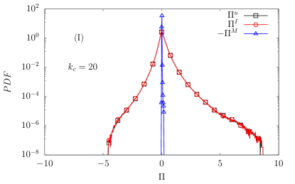
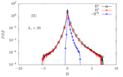
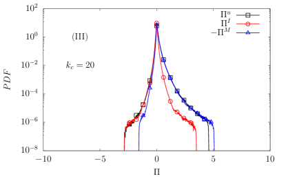
Figure 10: Fluctuations of $\Pi^{I}$ and $\Pi^{M}$ during kinematic (I), non-linear (II) and stationary (III) stages at $k_{c}=20$.

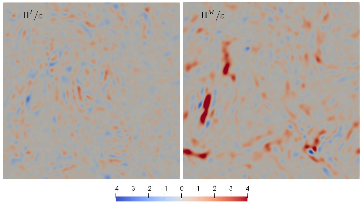
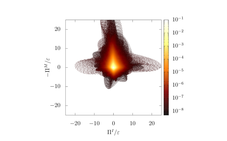
Figure 11: (Colour online) Top: Two-dimensional visualisations of the inertial and Maxwell SGS energy transfers $\Pi^{I}$ (left) and $-\Pi^{M}$ (right) at $k_{c}=20$ in stage (III). Positive values correspond to forward energy transfer while negative values incicate backscatter. Bottom: Corresponding joint pdf of $\Pi^{I}$ and $-\Pi^{M}$.

The clear forward transfer of energy in stage (III) associated with the Maxwell stress is also visible in the 2D visualisations of $\Pi^{I}$ and $\Pi^{M}$ presented in the top panels of Fig. 11. Unlike $\Pi^{I}$, $\Pi^{M}$ shows very intense and localized regions of forward transfer. As discussed earlier, the pdf of $\Pi^{I}$ becomes quite symmetric in stage (III), indicating that positive and negative fluctuations of $\Pi^{I}$ occur with similar probabilities. This is also visible in the visualisations, where we see regions of forward and inverse transfer which are of comparable intensity. The fluctuations of $\Pi^{I}$ also appear to be much weaker than those of $\Pi^{M}$. Finally, we find that $\Pi^{I}$ and $\Pi^{M}$ have a relation of weak inverse proportionality as can be seen from their joint pdf presented in the bottom panel of Fig. 11. The latter suggests that the transfer of kinetic energy between resolved scales and SGS is more likely to occur separately through $\Pi^{I}$ or $\Pi^{M}$ rather than simultaneously through both.

V Conclusions

In this paper, we investigated the different components of the SGS energy transfer through three stages of dynamo evolution considering mean and fluctuating properties. We decomposed the total SGS energy transfer in the components corresponding to either the momentum or the induction equation, thus separating kinetic from magnetic SGS energy transfer. The kinetic SGS energy transfer was then further split into an inertial component and a component originating from the Lorentz force. By also distinguishing between the actual SGS energy transfers and residual contributions from interactions amongst the resolved scales, we got clear measurements of the fluctuating individual SGS energy transfers.

Concerning the velocity field, important differences are present between the statistical properties of the inertial SGS energy transfer in presence of a saturated dynamo and in the nonconducting case. First, the kinetic energy cascade is depleted in the saturated dynamo regime, see Figs. 8(a) and 10. Second, we find that the pdf of the inertial SGS energy transfer becomes more symmetric and less Gaussian than in the non-conducting case with wider tails suggesting more extreme events also in terms of backscatter, see Figs. 9(a) and 10. Third, we found quantitative evidence that the flatness of the inertial SGS energy transfer has a weaker scale dependence, which suggests that the velocity field may be less intermittent in presence of a saturated small-scale dynamo than in the nonconducting case, see Fig. 9(c). This latter case deserves a more quantitative investigation by increasing the statistics and by extension of the involved scales. Concerning the magnetic field, we find that the pdf of the magnetic energy transfer is pretty symmetric in both the nonlinear and the saturated dynamo regimes, see Fig. 6(b). In contrast, the SGS energy transfer originating from the Maxwell stress in the momentum equation is clearly skewed towards positive values, see Figs. 9(b) and 10.

In terms of fundamental results on interscale energy transfer in MHD turbulence, the filtering technique is a useful alternative to spectral approaches. According to analyses of shell-to-shell transfers, magnetic and velocity-field modes couple at disparate wave number shells Verma04 ; Alexakis05a ; Mininni05a ; Alexakis07 , leading to nonlocal contributions to the conversion of kinetic to magnetic energy in Fourier space. As can be seen from Eqs. (III.1) and (III.1), the conversion of resolved-scale kinetic to magnetic energy involves resolved scales only. Although not assessed here, the energy conversion term for the SGS energies is also closed in terms of the SGS Aluie17 . That is, the conversion terms do not couple the resolved scales with the SGS. In summary, the filtering technique shows that energy conversion across the filter scale does not occur Aluie17 . The degree of locality of energy cascades is certainly affected by the presence of large-scale fields, such as in rotating turbulence, two-dimensional flows or in the presence of magnetic and kinetic helicity Alexakis18 , requiring further analysis of the effect of SGS closures on higher-order statistics Linkmann18 . Hence, separate a-priori studies are required in order to provide guidance for LES modeling in such cases, as e.g for large-scale dynamos Kessar16 .

In terms of guidance for LES modelling, the symmetry of the magnetic SGS energy transfer pdf implies that backscatter events are important, which calls applications of dissipative models for the stresses in the induction equation into question. For the momentum equation, a similar situation occurs for the inertial SGS energy transfer in the saturated stage of the dynamo. As a result, while a dissipative model for the inertial stresses may be suitable during the kinematic stage, a more sophisticated approach is required to adequately capture the increased backscatter in the nonlinear and saturated stages. On the other hand, dissipative models would be well suited for the Maxwell stress in both nonlinear and saturated stages. Finally, we find that the correlation between the individual SGS energy transfers appears to be of inverse proportionality in the saturated stage. This holds for $\Pi^{u}$ and $\Pi^{b}$ and also for $\Pi^{I}$ and $\Pi^{M}$. That is, the energy transfers in the different channels appear to occur separately, which should be taken into account in the design of more sophisticated LES models for MHD. However, measurements of the correlations between the different SGS energy transfers at higher Reynolds numbers need to be carried out in order to better quantify the effect.

Appendix A Comparison between the SGS and Leonard energy transfers

The Leonard components of the individual energy transfer terms were defined in Eqs. (24)-(25). As mentioned before, the Leonard transfers do not contribute to the SGS energy transfer as they are closed in terms of the resolved fields. Furthermore, it can be shown that they vanish under spatial averaging. The latter suggests that forward and backward energy transfer should be more or less equally likely. Figure 12 presents comparisons between the actual SGS energy transfer $\Pi$ and its Leonard component $\Pi^{L}$ at $k_{c}=20$ and during stages (I)-(III). As can be seen, $\Pi^{L}$ is indeed more symmetric than $\Pi$ in all cases. This situation is also present for the Maxwell energy transfers $\Pi^{M}$ and $\Pi^{M,L}$ shown in Fig. 13 for the nonlinear and stationary stages of dynamo evolution. At least in stage (III), a measurement of $\Pi^{M}+\Pi^{M,L}$ instead of $\Pi^{M}$ would have resulted in a more pronounced left tail of the pdf, leading to the consclusion of more backscatter being present in the Maxwell SGS transfer than there actually is. In Fig. 14 the same measurements of the Maxwell energy transfers are presented at a different cutoff closer to the dissipation range, namely $k_{c}=80$. At this scale, all pdfs show a higher probability to measure extreme events of energy transfer. However, the pdf of the Maxwell energy transfer $\Pi^{M}$ remains clearly skewed towards the right, which suggests that the extreme events remain correlated to the direction of the mean energy flux, even though they become more than two orders of magnitude larger compared to the mean value. Moreover, as already observed in Fig.12 from the pdfs of the total energy transfer, this information is not accessible through a measurement of the sum between $\Pi^{M}$ and $\Pi^{M,L}$, because the Leonard term is completely symmetric and large enough to dominate the left tail of the PDF. The same results are valid in both the nonlinear and the stationary stage.

Figure 12: pdfs of $\Pi$ and $\Pi^{L}$ at the kinematic stage (I), non-linear stage (II) and the stationary stage (III), with $k_{c}=20$.

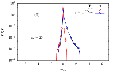
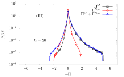
Figure 13: pdfs of the Maxwell SGS energy transfers $\Pi^{M}$ and $\Pi^{M,L}$ and their sum in the nonlinear (II) and the stationary (III) stages, with $k_{c}=20$.

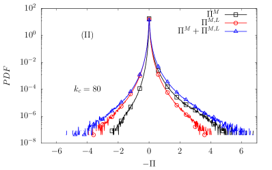
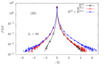
Figure 14: pdfs of the Maxwell SGS energy transfers $\Pi^{M}$ and $\Pi^{M,L}$ and their sum in the nonlinear (II) and the stationary (III) stages, with $k_{c}=80$.

References

- [1] U. Frisch. Turbulence: The Legacy of Kolmogorov. Cambridge University Press, 1995.
- [2] L. D. Landau and E. M. Lifshitz. Fluid Mechanics. Pergamon Press, London, English edition, 1959.
- [3] U. Piomelli. Large-eddy simulation: achievements and challenges. Prog. Aerosp. Sci., 35(4):335–362, 1999.
- [4] C. Meneveau and J. Katz. Scale-invariance and turbulence models for large-eddy simulation. Annu. Rev. Fluid Mech., 32(1):1–32, 2000.
- [5] S. B. Pope. Turbulent flows. IOP Publishing, 2001.
- [6] M. Miesch, W. Matthaeus, A. Brandenburg, A. Petrosyan, A. Pouquet, C. Cambon, F. Jenko, D. Uzdensky, J. Stone, S. Tobias, et al. Large-eddy simulations of magnetohydrodynamic turbulence in heliophysics and astrophysics. Space Sci. Rev., 194(1-4):97–137, 2015.
- [7] H. Aluie. Coarse-grained incompressible magnetohydrodynamics: analyzing the turbulent cascades. New J. Physics, 19(2):025008, 2017.
- [8] M. Kessar, G. Balarac, and F. Plunian. The effect of subgrid-scale models on grid-scale/subgrid-scale energy transfers in large-eddy simulation of incompressible magnetohydrodynamic turbulence. Phys. Plasmas, 23(10):102305, 2016.
- [9] Y. Zhou and G. Vahala. Aspects of subgrid modelling and large-eddy simulation of magnetohydrodynamic turbulence. J. Plasma Phys., 45(2):239–249, 1991.
- [10] M. L. Theobald, P. A. Fox, and S. Sofia. A subgrid-scale resistivity for magnetohydrodynamics. Phys. Plasmas, 1(9):3016–3032, 1994.
- [11] O. Agullo, W.-C. Müller, B. Knaepen, and D. Carati. Large eddy simulation of decaying magnetohydrodynamic turbulence with dynamic subgrid-modeling. Phys. Plasmas, 8(7):3502–3505, 2001.
- [12] W.-C. Müller and D. Carati. Dynamic gradient-diffusion subgrid models for incompressible magnetohydrodynamic turbulence. Phys. Plasmas, 9(3):824–834, 2002.
- [13] W.-C. Müller and D. Carati. Large-eddy simulation of magnetohydrodynamic turbulence. Comput. Phys. Commun., 147(1-2):544–547, 2002.
- [14] B. Knaepen and P. Moin. Large-eddy simulation of conductive flows at low magnetic reynolds number. Phys. Fluids, 16(5):1255–1261, 2004.
- [15] N. E. L. Haugen and A. Brandenburg. Hydrodynamic and hydromagnetic energy spectra from large eddy simulations. Phys. Fluids, 18(7):075106, 2006.
- [16] J. Baerenzung, H. Politano, Y. Ponty, and A. Pouquet. Spectral modeling of turbulent flows and the role of helicity. Phys. Rev. E, 77(4):046303, 2008.
- [17] G. Balarac, A. G. Kosovichev, O. Brugière, A. A. Wray, and N. N. Mansour. Modeling of the subgrid-scale term of the filtered magnetic field transport equation. In Proceedings of Summer Program 2010, pages 503–512. Center for Turbulence Research, Stanford University, 2010.
- [18] A. A. Chernyshov, K. V. Karelsky, and A. S. Petrosyan. Forced turbulence in large-eddy simulation of compressible magnetohydrodynamic turbulence. Phys. Plasmas, 17(10):102307, 2010.
- [19] D. Biskamp. Magnetohydrodynamic Turbulence. Cambridge University Press, 1st edition, 2003.
- [20] M. K. Verma. Statistical theory of magnetohydrodynamic turbulence: recent results. Phys. Rep., 401:229–380, 2004.
- [21] S. Cerutti and C. Meneveau. Intermittency and relative scaling of subgrid-scale energy dissipation in isotropic turbulence. Phys. Fluids, 10(4):928–937, 1998.
- [22] M. Buzzicotti, M. Linkmann, H. Aluie, L. Biferale, J. Brasseur, and C. Meneveau. Effect of filter type on the statistics of energy transfer between resolved and subfilter scales from a-priori analysis of direct numerical simulations of isotropic turbulence. J. Turbul., 19(2):167–197, 2018.
- [23] H. Politano and A. Pouquet. Model of intermittency in magnetohydrodynamic turbulence. Phys. Rev. E, 52:636, 1995.
- [24] S. Servidio, W. H. Matthaeus, M. A. Shay, P. A. Cassak, and P. Dmitruk. Magnetic reconnection in two-dimensional magnetohydrodynamic turbulence. Phys. Rev. Lett., 102(11):115003, 2009.
- [25] P. D. Mininni and A. G. Pouquet. Finite dissipation and intermittency in magnetohydrodynamics. Phys. Rev. E., 80:025401, 2009.
- [26] G. Sahoo, P. Perlekar, and R. Pandit. Systematics of the magnetic-prandtl-number dependence of homogeneous, isotropic magnetohydrodynamic turbulence. New J. Phys., 13(1):013036, 2011.
- [27] K. Yoshimatsu, K. Schneider, N. Okamoto, Y. Kawahara, and M. Farge. Intermittency and geometrical statistics of three-dimensional homogeneous magnetohydrodynamic turbulence: A wavelet viewpoint. Phys. Plasmas, 18(9):092304, 2011.
- [28] P. Rodriguez Imazio, L. N. Martin, P. Dmitruk, and P. D. Mininni. Intermittency in hall-magnetohydrodynamics with a strong guide field. Phys. Plasmas, 20(5):052506, 2013.
- [29] R. Meyrand, K. H. Kiyani, and S. Galtier. Weak magnetohydrodynamic turbulence and intermittency. J. Fluid Mech., 770, 2015.
- [30] Y. Yang, W. H. Matthaeus, Y. Shi, M. Wan, and S. Chen. Compressibility effect on coherent structures, energy transfer, and scaling in magnetohydrodynamic turbulence. Phys. Fluids, 29(3):035105, 2017.
- [31] P. Veltri. MHD turbulence in the solar wind: self-similarity, intermittency and coherent structures. Plasma Phys. Controlled Fusion, 41(3A):A787, 1999.
- [32] C. Salem, A. Mangeney, S. D. Bale, and P. Veltri. Solar wind magnetohydrodynamics turbulence: anomalous scaling and role of intermittency. Astrophys. J., 702(1):537, 2009.
- [33] M. Wan, K. T. Osman, W. H. Matthaeus, and S. Oughton. Investigation of intermittency in magnetohydrodynamics and solar wind turbulence: scale-dependent kurtosis. Astrophys. J., 744(2):171, 2011.
- [34] W. H. Matthaeus, M. Wan, S. Servidio, A. Greco, K. T. Osman, S. Oughton, and P. Dmitruk. Intermittency, nonlinear dynamics and dissipation in the solar wind and astrophysical plasmas. Phil. Trans. R. Soc. A, 373(2041):20140154, 2015.
- [35] P. Grete, D. G. Vlaykov, W. Schmidt, and D. R. G Schleicher. A nonlinear structural subgrid-scale closure for compressible MHD. II. A priori comparison on turbulence simulation data. Phys. Plasmas, 23(6):062317, 2016.
- [36] P. Grete, D. G. Vlaykov, W. Schmidt, D. R. G. Schleicher, and C. Federrath. Nonlinear closures for scale separation in supersonic magnetohydrodynamic turbulence. New J. Phys., 17:023070, 2015.
- [37] S. A. Orszag. Numerical methods for the simulation of turbulence. Phys. Fluids, 12(12):II–250, 1969.
- [38] S. A. Orszag. On the elimination of aliasing in finite-difference schemes by filtering high-wavenumber components. J. Atmos. Sci., 28(6):1074–1074, 1971.
- [39] N. E. L. Haugen, A. Brandenburg, and W. Dobler. Simulations of nonhelical hydromagnetic turbulence. Phys. Rev. E, 70(1):016308, 2004.
- [40] A. A. Schekochihin, S. C. Cowley, S. F. Taylor, J. L. Maron, and J. C. McWilliams. Simulations of the Small-Scale Turbulent Dynamo. Astrophys. J., 612(1):276, 2004.
- [41] N. E. L. Haugen, A. Brandenburg, and W. Dobler. Is nonhelical hydromagnetic turbulence peaked at small scales? Astrophys. J. Lett., 597:L141, 2003.
- [42] A. Brandenburg. Magnetic Prandtl number dependence of the kinetic-to-magnetic dissipation ratio. Astrophys. J., 791:1–10, 2014.
- [43] M. Linkmann, A. Berera, and E. E. Goldstraw. Reynolds-number dependence of the dimensionless dissipation rate in homogeneous magnetohydrodynamic turbulence. Phys. Rev. E, 95:013102, 2017.
- [44] M. E. McKay, M. Linkmann, D. Clark, A. A. Chalupa, and A. Berera. Comparison of forcing functions in magnetohydrodynamics. Phys. Rev. Fluids, 2:114604, 2017.
- [45] P. D. Mininni, A. Alexakis, and A. Pouquet. Shell-to-shell energy transfer in magnetohydrodynamics. II. Kinematic dynamo. Phys. Rev. E, 72:046302, 2005.
- [46] A. Brandenburg and K. Subramanian. Astrophysical magnetic fields and nonlinear dynamo theory. Physics Reports, 417:1–209, 2005.
- [47] Y. Yang, Y. Shi, M. Wan, W. H. Matthaeus, and S. Chen. Energy cascade and its locality in compressible magnetohydrodynamic turbulence. Phys. Rev. E, 93:061102, 2016.
- [48] P. Sagaut. Large Eddy Simulations for Incompressible Flows: An Introduction. Springer, 2006.
- [49] H. Aluie and G. L. Eyink. Localness of energy cascade in hydrodynamic turbulence. I. Smooth coarse graining. Phys. Fluids, 21:115107, 2009.
- [50] H. Aluie and G. L. Eyink. Localness of energy cascade in hydrodynamic turbulence. II. Sharp spectral filter. Phys. Fluids, 21:115108, 2009.
- [51] A. Leonard. Energy cascade in large-eddy simulations of turbulent fluid flows. Advances in geophysics, 18:237–248, 1975.
- [52] S. S. Ray, U. Frisch, S. Nazarenko, and T. Matsumoto. Resonance phenomenon for the Galerkin-truncated Burgers and Euler equations. Phys. Rev. E, 84(1):016301, 2011.
- [53] B. Vreman, B. Geurts, and H. Kuerten. Realizability conditions for the turbulent stress tensor in large-eddy simulation. J. Fluid Mech., 278:351–362, 1994.
- [54] G. L. Eyink. Locality of turbulent cascades. Physica D: Nonlinear Phenomena, 207(1-2):91–116, 2005.
- [55] Z.-S. She and E. Leveque. Universal scaling laws in fully developed turbulence. Phys. Rev. Lett., 72(3):336, 1994.
- [56] G. L. Eyink. The ‘Multifractal Model’of Turbulence and A Priori Estimates in Large-Eddy Simulation, II. Evaluation of Stress Models and Non-Universal Effects of the Filter. arXiv preprint chao-dyn/9602019, 1996.
- [57] J. Smagorinsky. General circulation experiments with the primitive equations: I. the basic experiment. Monthly weather review, 91:99–164, 1963.
- [58] T. Gotoh, D. Fukayama, and T. Nakano. Velocity field statistics in homogeneous steady turbulence obtained using a high-resolution direct numerical simulation. Phys. Fluids, 14:1065, 2002.
- [59] G. L. Eyink. The Multifractal Model of Turbulence and A Priori Estimates in Large-Eddy Simulation, I. Subgrid Flux and Locality of Energy Transfer. arxiv:9602018v1, 1996.
- [60] A. Alexakis, P. D. Mininni, and A. Pouquet. Shell-to-shell energy transfer in magnetohydrodynamics. I. Steady state turbulence. Phys. Rev. E, 72:046301, 2005.
- [61] A. Alexakis, P. D. Mininni, and A. Pouquet. Turbulent cascades, transfer, and scale interactions in magnetohydrodynamics. New J. Phys., 9:298, 2007.
- [62] A. Alexakis and L. Biferale. Cascades and transitions in turbulent flows. Phys. Rep., 767-769:1–101, 2018.
- [63] M. Linkmann, M. Buzzicotti, and L. Biferale. Multi-scale properties of large eddy simulations: correlations between resolved-scale velocity-field increments and subgrid-scale quantities. J. Turbul., 19:493–527, 2018.