Preventing Unnecessary Groundings in the Lifted Dynamic Junction Tree Algorithm

Abstract

The lifted dynamic junction tree algorithm (LDJT) efficiently answers filtering and prediction queries for probabilistic relational temporal models by building and then reusing a first-order cluster representation of a knowledge base for multiple queries and time steps. Unfortunately, a non-ideal elimination order can lead to groundings even though a lifted run is possible for a model. We extend LDJT (i) to identify unnecessary groundings while proceeding in time and (ii) to prevent groundings by delaying eliminations through changes in a temporal first-order cluster representation. The extended version of LDJT answers multiple temporal queries orders of magnitude faster than the original version.

1 Introduction

Areas like healthcare, logistics or even scientific publishing deal with probabilistic data with relational and temporal aspects and need efficient exact inference algorithms. These areas involve many objects in relation to each other with changes over time and uncertainties about object existence, attribute value assignments, or relations between objects. More specifically, publishing involves publications (the relational part) for many authors (the objects), streams of papers over time (the temporal part), and uncertainties for example due to missing or incomplete information. By performing model counting, probabilistic databases can answer queries for relational temporal models with uncertainties (?; ?). However, each query embeds a process behaviour, resulting in huge queries with possibly redundant information. In contrast to PDBs, we build more expressive and compact models including behaviour (offline) enabling efficient answering of more compact queries (online). For query answering, our approach performs deductive reasoning by computing marginal distributions at discrete time steps. In this paper, we study the problem of exact inference and investigate how to prevent unnecessary groundings in large temporal probabilistic models that exhibit symmetries.

We propose parameterised probabilistic dynamic models to represent probabilistic relational temporal behaviour and introduce the LDJT to exactly answer multiple filtering and prediction queries for multiple time steps efficiently (?). LDJT combines the advantages of the interface algorithm (?) and the lifted junction tree algorithm (LJT) (?). Specifically, this paper extends LDJT and contributes (i) means to identify whether groundings occur and (ii) an approach to prevent unnecessary groundings by extending inter first-order junction tree (FO jtree) separators.

LDJT reuses an FO jtree structure to answer multiple queries and reuses the structure to answer queries for all time steps $t>0$. Additionally, LDJT ensures a minimal exact inter FO jtree information propagation over a separator. Unfortunately, due to a non-ideal elimination order unnecessary groundings can occur. In the static case, LJT prevents groundings by fusing parclusters, the nodes of an FO jtree. For the temporal case, fusing parclusters is not applicable, as LDJT would need to fuse parclusters of different FO jtrees. We propose to prevent groundings by extending inter FO jtree separators and thereby changing the elimination order by delaying eliminations to the next time step.

The remainder of this paper has the following structure: We begin by recapitulating PDMs as a representation for relational temporal probabilistic models and present LDJT, an efficient reasoning algorithm for PDMs. Afterwards, we present LJT’s techniques to prevent unnecessary groundings and extend LDJT to prevent unnecessary groundings. Lastly, we evaluate the extended version of LDJT against LDJT’s orignal version and LJT. We conclude by looking at possible extensions.

2 Related Work

We take a look at inference for propositional temporal models, relational static models, and give an overview about relational temporal model research.

For exact inference on propositional temporal models, a naive approach is to unroll the temporal model for a given number of time steps and use any exact inference algorithm for static, i.e., non-temporal, models. In the worst case, once the number of time steps changes, one has to unroll the model and infer again. Murphy (?) proposes the interface algorithm consisting of a forward and backward pass that uses a temporal d-separation with a minimal set of nodes to apply static inference algorithms to the dynamic model.

First-order probabilistic inference leverages the relational aspect of a static model. For models with known domain size, first-order probabilistic inference exploits symmetries in a model by combining instances to reason with representatives, known as lifting (?). Poole (?) introduces parametric factor graphs as relational models and proposes lifted variable elimination (LVE) as an exact inference algorithm on relational models. Further, de Salvo Braz (?), Milch et al. (?), and Taghipour et al. (?) extend LVE to its current form. Lauritzen and Spiegelhalter (?) introduce the junction tree algorithm. To benefit from the ideas of the junction tree algorithm and LVE, Braun and Möller (?) present LJT, which efficiently performs exact first-order probabilistic inference on relational models given a set of queries.

To handle inference for relational temporal models most approaches are approximative. Additional to being approximative, these approaches involve unnecessary groundings or are only designed to handle single queries efficiently. Ahmadi et al. (?) propose lifted (loopy) belief propagation. From a factor graph, they build a compressed factor graph and apply lifted belief propagation with the idea of the factored frontier algorithm (?), which is an approximate counterpart to the interface algorithm. Thon et al. (?) introduce CPT-L, a probabilistic model for sequences of relational state descriptions with a partially lifted inference algorithm. Geier and Biundo (?) present an online interface algorithm for dynamic Markov logic networks, similar to the work of Papai et al. (?). Both approaches slice DMLNs to run well-studied static MLN (?) inference algorithms on each slice individually. Two ways of performing online inference using particle filtering are described in (?; ?).

Vlasselaer et al. (?; ?) introduce an exact approach, which involves computing probabilities of each possible interface assignment on a ground level.

3 Parameterised Probabilistic Models

Based on (?), we present parameterised probabilistic models for relational static models. Afterwards, we extend PMs to the temporal case, resulting in PDMs for relational temporal models, which, in turn, are based on (?).

3.1 Parameterised Probabilistic Models

PMs combine first-order logic with probabilistic models, representing first-order constructs using logical variables as parameters.

Definition 1.

Let $\mathbf{L}$ be a set of logvar names, $\Phi$ a set of factor names, and $\mathbf{R}$ a set of random variable (randvar) names. A parameterised randvar (PRV) $A=P(X^{1},...,X^{n})$ represents a set of randvars behaving identically by combining a randvar $P\in\mathbf{R}$ with $X^{1},...,X^{n}\in\mathbf{L}$. If $n=0$, the PRV is parameterless. The domain of a logvar $L$ is denoted by $\mathcal{D}(L)$. The term $range(A)$ provides possible values of a PRV $A$. Constraint $(\mathbf{X},C_{\mathbf{X}})$ allows to restrict logvars to certain domain values and is a tuple with a sequence of logvars $\mathbf{X}=(X^{1},...,X^{n})$ and a set $C_{\mathbf{X}}\subseteq\times_{i=1}^{n}\mathcal{D}(X^{i})$. $\top$ denotes that no restrictions apply and may be omitted. The term $lv(Y)$ refers to the logvars in some element $Y$. The term $gr(Y)$ denotes the set of instances of $Y$ with all logvars in $Y$ grounded w.r.t. constraints.

Let us set up a PM for publications on some topic. We model that the topic may be hot, conferences are attractive, people do research, and publish in publications. From $\mathbf{R}=\{Hot,DoR\}$ and $\mathbf{L}=\{A,P,X\}$ with $\mathcal{D}(A)=\{a_{1},a_{2}\}$, $\mathcal{D}(P)=\{p_{1},p_{2}\}$, and $\mathcal{D}(X)=\{x_{1},x_{2},x_{3}\}$, we build the boolean PRVs $Hot$ and $DoR(X)$. With $C=(X,\{x_{1},x_{2}\})$, $gr(DoR(X)|C)=\{DoR(x_{1}),DoR(x_{2})\}$.

Definition 2.

We denote a parametric factor (parfactor) $g$ with $\forall\mathbf{X}:\phi(\mathcal{A})\;|C$. $\mathbf{X}\subseteq\mathbf{L}$ being a set of logvars over which the factor generalises and $\mathcal{A}=(A^{1},...,A^{n})$ a sequence of PRVs. We omit $(\forall\mathbf{X}:)$ if $\mathbf{X}=lv(\mathcal{A})$. A function $\phi:\times_{i=1}^{n}range(A^{i})\mapsto\mathbb{R}^{+}$ with name $\phi\in\Phi$ is defined identically for all grounded instances of $\mathcal{A}$. A list of all input-output values is the complete specification for $\phi$. $C$ is a constraint on $\mathbf{X}$. A PM $G:=\{g^{i}\}_{i=0}^{n-1}$ is a set of parfactors and semantically represents the full joint probability distribution $P(G)=\frac{1}{Z}\prod_{f\in gr(G)}\phi(\mathcal{A}_{f})$ where $Z$ is a normalisation constant.

Figure 1: Parfactor graph for $G^{ex}$

Figure 2: $G_{\rightarrow}^{ex}$ the two-slice temporal parfactor graph for model $G^{ex}$

Adding boolean PRVs $Pub(X,P)$ and $AttC(A)$, $G_{ex}=\{g^{i}\}^{1}_{i=0}$, $g^{0}=\phi^{0}(Pub(X,P),AttC(A),Hot)$, $g^{1}=\phi^{1}(DoR(X),AttC(A),Hot)$ forms a model. All parfactors have eight input-output pairs (omitted). Constraints are $\top$, i.e., the $\phi$’s hold for all domain values. E.g., $gr(g^{1})$ contains four factors with identical $\phi$. Figure 1 depicts $G^{ex}$ as a graph with four variable nodes for the PRVs and two factor nodes for $g^{0}$ and $g^{1}$ with edges to the PRVs involved. Additionally, we can observe the attractiveness of conferences. The remaining PRVs are latent.

The semantics of a model is given by grounding and building a full joint distribution. In general, queries ask for a probability distribution of a randvar using a model’s full joint distribution and fixed events as evidence.

Definition 3.

Given a PM $G$, a ground PRV $Q$ and grounded PRVs with fixed range values $\mathbf{E}$, the expression $P(Q|\mathbf{E})$ denotes a query w.r.t. $P(G)$.

3.2 Parameterised Probabilistic Dynamic Models

To define PDMs, we use PMs and the idea of how Bayesian networks give rise to dynamic Bayesian networks. We define PDMs based on the first-order Markov assumption, i.e., a time slice $t$ only depends on the previous time slice $t-1$. Further, the underlining process is stationary, i.e., the model behaviour does not change over time.

Definition 4.

A PDM is a pair of PMs $(G_{0},G_{\rightarrow})$ where $G_{0}$ is a PM representing the first time step and $G_{\rightarrow}$ is a two-slice temporal parameterised model representing $\mathbf{A}_{t-1}$ and $\mathbf{A}_{t}$ where $\mathbf{A}_{\pi}$ is a set of PRVs from time slice $\pi$.

Figure 2 shows how the model $G^{ex}$ behaves over time. $G_{\rightarrow}^{ex}$ consists of $G^{ex}$ for time step $t-1$ and for time step $t$ with inter-slice parfactor for the behaviour over time. In this example, the parfactor $g^{H}$ is the inter-slice parfactors.

Definition 5.

Given a PDM $G$, a ground PRV $Q_{t}$ and grounded PRVs with fixed range values $\mathbf{E}_{0:t}$ the expression $P(Q_{t}|\mathbf{E}_{0:t})$ denotes a query w.r.t. $P(G)$.

The problem of answering a marginal distribution query $P(A^{i}_{\pi}|\mathbf{E}_{0:t})$ w.r.t. the model is called prediction for $\pi>t$ and filtering for $\pi=t$.

4 Lifted Dynamic Junction Tree Algorithm

To provide means to answer queries for PMs, we introduce LJT, mainly based on (?). Afterwards, we present LDJT (?) consisting of FO jtree constructions for a PDM and a filtering and prediction algorithm.

4.1 Lifted Junction Tree Algorithm

LJT provides efficient means to answer queries $P(\mathbf{Q}|\mathbf{E})$, with a set of query terms, given a PM $G$ and evidence $\mathbf{E}$, by performing the following steps: (i) Construct an FO jtree $J$ for $G$. (ii) Enter $\mathbf{E}$ in $J$. (iii) Pass messages. (iv) Compute answer for each query $Q^{i}\in\mathbf{Q}$. We first define an FO jtree and then go through each step. To define an FO jtree, we need to define parameterised clusters (parclusters), the nodes of an FO jtree.

Definition 6.

A parcluster $\mathbf{C}$ is defined by $\forall\mathbf{L}:\mathbf{A}|C$. $\mathbf{L}$ is a set of logvars, $\mathbf{A}$ is a set of PRVs with $lv(\mathbf{A})\subseteq\mathbf{L}$, and $C$ a constraint on $\mathbf{L}$. We omit $(\forall\mathbf{L}:)$ if $\mathbf{L}=lv(\mathbf{A})$. A parcluster $\mathbf{C}^{i}$ can have parfactors $\phi(\mathcal{A}^{\phi})|C^{\phi}$ assigned given that (i) $\mathcal{A}^{\phi}\subseteq\mathbf{A}$, (ii) $lv(\mathcal{A}^{\phi})\subseteq\mathbf{L}$, and (iii) $C^{\phi}\subseteq C$ holds. We call the set of assigned parfactors a local model $G^{i}$.
An FO jtree for a model $G$ is $J=(\mathbf{V},\mathbf{E})$ where $J$ is a cycle-free graph, the nodes $\mathbf{V}$ denote a set of parcluster, and the set $\mathbf{E}$ edges between parclusters. An FO jtree must satisfy the following properties: (i) A parcluster $\mathbf{C}^{i}$ is a set of PRVs from $G$. (ii) For each parfactor $\phi(\mathcal{A})|C$ in G, $\mathcal{A}$ must appear in some parcluster $\mathbf{C}^{i}$. (iii) If a PRV from $G$ appears in two parclusters $\mathbf{C}^{i}$ and $\mathbf{C}^{j}$, it must also appear in every parcluster $\mathbf{C}^{k}$ on the path connecting nodes i and j in $J$. The separator $\mathbf{S}^{ij}$ of edge $i-j$ is given by $\mathbf{C}^{i}\cap\mathbf{C}^{j}$ containing shared PRVs.

Figure 3: FO jtree for $G^{ex}$ (local models in grey)

LJT constructs an FO jtree using a first-order decomposition tree (FO dtree), enters evidence in the FO jtree, and passes messages through an inbound and an outbound pass, to distribute local information of the nodes through the FO jtree. To compute a message, LJT eliminates all non-seperator PRVs from the parcluster’s local model and received messages. After message passing, LJT answers queries. For each query, LJT finds a parcluster containing the query term and sums out all non-query terms in its local model and received messages.

Figure 3 shows an FO jtree of $G^{ex}$ with the local models of the parclusters and the separators as labels of edges. During the inbound phase of message passing, LJT sends messages from $\mathbf{C}^{1}$ to $\mathbf{C}^{2}$ and for the outbound phase a message from $\mathbf{C}^{2}$ to $\mathbf{C}^{1}$. If we want to know whether $Hot$ holds, we query for $P(Hot)$ for which LJT can use either parcluster $\mathbf{C}^{1}$ or $\mathbf{C}^{2}$. Thus, LJT can sum out $AttC(A)$ and $DoR(X)$ from $\mathbf{C}^{2}$’s local model $G^{2}$, $\{g^{1}\}$, combined with the received messages, here, one message from $\mathbf{C}^{1}$.

4.2 LDJT: Overview

LDJT efficiently answers queries $P(\mathbf{Q}_{t}|\mathbf{E}_{0:t})$, with a set of query terms $\{\mathbf{Q}_{t}\}_{t=0}^{T}$, given a PDM $G$ and evidence $\{\mathbf{E}_{t}\}_{t=0}^{T}$, by performing the following steps: (i) Construct offline two FO jtrees $J_{0}$ and $J_{t}$ with in- and out-clusters from $G$. (ii) For $t=0$, using $J_{0}$ to enter $\mathbf{E}_{0}$, pass messages, answer each query term $Q_{\pi}^{i}\in\mathbf{Q}_{0}$, and preserve the state. (iii) For $t>0$, instantiate $J_{t}$ for the current time step $t$, recover the previous state, enter $\mathbf{E}_{t}$ in $J_{t}$, pass messages, answer each query term $Q_{\pi}^{i}\in\mathbf{Q}_{t}$, and preserve the state.

Next, we show how LDJT constructs the FO jtrees $J_{0}$ and $J_{t}$ with in- and out-clusters, which contain a minimal set of PRVs to m-separate the FO jtrees. M-separation means that information about these PRVs make FO jtrees independent from each other. Afterwards, we present how LDJT connects the FO jtrees for reasoning to solve the filtering and prediction problems efficiently.

4.3 LDJT: FO Jtree Construction for PDMs

LDJT constructs FO jtrees for $G_{0}$ and $G_{\rightarrow}$, both with an incoming and outgoing interface. To be able to construct the interfaces in the FO jtrees, LDJT uses the PDM $G$ to identify the interface PRVs $\mathbf{I}_{t}$ for a time slice $t$.

Definition 7.

The forward interface is defined as $\mathbf{I}_{t}=\{A_{t}^{i}\mid\exists\phi(\mathcal{A})|C\in G:A_{t}^{i}\in\mathcal{A}\wedge\exists A_{t+1}^{j}\in\mathcal{A}\}$, i.e., the PRVs which have successors in the next slice.

For $G_{\rightarrow}^{ex}$, which is shown in Fig. 2, PRVs $Hot_{t-1}$ and $Pub_{t-1}(X,P)$ have successors in the next time slice, making up $\mathbf{I}_{t-1}$. To ensure interface PRVs $\mathbf{I}$ ending up in a single parcluster, LDJT adds a parfactor $g^{I}$ over the interface to the model. Thus, LDJT adds a parfactor $g^{I}_{0}$ over $\mathbf{I}_{0}$ to $G_{0}$, builds an FO jtree $J_{0}$ and labels the parcluster with $g^{I}_{0}$ from $J_{0}$ as in- and out-cluster. For $G_{\rightarrow}$, LDJT removes all non-interface PRVs from time slice $t-1$, adds parfactors $g^{I}_{t-1}$ and $g^{I}_{t}$, constructs $J_{t}$. Further, LDJT labels the parcluster containing $g^{I}_{t-1}$ as in-cluster and labels the parcluster containing $g^{I}_{t}$ as out-cluster.

The interface PRVs are a minimal required set to m-separate the FO jtrees. LDJT uses these PRVs as separator to connect the out-cluster of $J_{t-1}$ with the in-cluster of $J_{t}$, allowing to reusing the structure of $J_{t}$ for all $t>0$.

4.4 LDJT: Proceeding in Time with the FO Jtree Structures

Figure 4: Forward and backward pass of LDJT (local models and labeling in grey)

Since $J_{0}$ and $J_{t}$ are static, LDJT uses LJT as a subroutine by passing on a constructed FO jtree, queries, and evidence for step $t$ to handle evidence entering, message passing, and query answering using the FO jtree. Further, for proceeding to the next time step, LDJT calculates an $\alpha_{t}$ message over the interface PRVs using the out-cluster to preserve the information about the current state. Afterwards, LDJT increases $t$ by one, instantiates $J_{t}$, and adds $\alpha_{t-1}$ to the in-cluster of $J_{t}$. During message passing, $\alpha_{t-1}$ is distributed through $J_{t}$.

Figure 4 depicts how LDJT uses the interface message passing between time step three to four. First, LDJT sums out the non-interface PRV $AttC_{3}(A)$ from $\mathbf{C}_{3}^{2}$’s local model and the received messages and saves the result in message $\alpha_{3}$. After increasing $t$ by one, LDJT adds $\alpha_{3}$ to the in-cluster of $J_{4}$, $\mathbf{C}_{4}^{1}$. $\alpha_{3}$ is then distributed by message passing and accounted for during calculating $\alpha_{4}$.

5 Preventing Groundings in LJT

A lifted solution to a query given a model means that we compute an answer without grounding a part of the model. Unfortunately, not all models have a lifted solution because LVE, the basis for LJT, requires certain conditions to hold. Therefore, these models involve groundings with any exact lifted inference algorithm. Grounding a logvar is expensive and, during message passing, may propagate through all nodes. LJT has a few approaches to prevent groundings for a static FO jtree. On the one hand, some approaches originate from LVE. On the other hand, LJT has a fuse operator to prevent groundings, occurring due to a non-ideal elimination order. Finding an optimal elimination order is in general NP-hard (?). This section is mainly based on (?).

5.1 General Grounding Prevention Techniques from LVE

One approach to prevent groundings is to perform lifted summing out. The idea is to compute VE for one case and exponentiate the result for isomorphic instances. Another approach in LVE to prevent groundings is count-conversion, which exploits that all randvars of a PRV $A$ evaluate to a value $v$ of $range(A)$. LVE forms a histogram by counting for each $v\in range(A)$ how many instances of $gr(A)$ evaluate to $v$. Let us start by defining counting randvar (CRV).

Definition 8.

$\#_{X\in C}[P(\mathbf{X})]$ denotes a CRV with PRV $P(\mathbf{X})$ and constraint $C$, where $lv(\mathbf{X})=\{X\}$. Its range is the space of possible histograms. If $\{X\}\subset lv(\mathbf{X})$, the CRV is a parameterised CRV (PCRV) representing a set of CRVs. Since counting binds logvar $X$, $lv(\#_{X\in C}[P(\mathbf{X})])=\mathbf{X}\setminus\{X\}$. We count-convert a logvar $X$ in a parfactor $g=\mathbf{L}:\phi(\mathcal{A})|C$ by turning a PRV $A^{i}\in\mathcal{A}$, $X\in lv(A^{i})$, into a CRV $A^{i^{\prime}}$. In the new parfactor $g^{\prime}$, the input for $A^{i^{\prime}}$ is a histogram $h$. Let $h(a^{i})$ denote the count of $a^{i}$ in $h$. Then, $\phi^{\prime}(...,a^{i-1},h,a^{i+1},...)$ maps to $\prod_{a^{i}\in range(A^{i})}\phi(...,a^{i-1},a^{i},a^{i+1},...)^{h(a^{i})}$.

One precondition to count-convert a logvar $X$ in $g$, is that only one input in $g$ contains $X$. To perform lifted summing out PRV $A$ from parfactor $g$, $lv(A)=lv(g)$. For the complete list of preconditions for both approaches, see (?).

5.2 Preventing Groundings during Intra FO Jtree Message Passing

During message passing, LJT eliminates PRVs by summing out. Thus, in case LJT cannot apply lifted summing out, it has to ground logvars. The messages LJT passes via the separators restrict the elimination order, which can lead to grounding, in case lifted summing out is not applicable.

LJT has three tests whether groundings occur during message passing. Roughly speaking, the first test checks if LJT can apply lifted summing out, the second test checks to prevent groundings by count-conversion, and the third test validates that a count-conversion will not result in groundings in another parcluster.

During message passing, a parcluster $\mathbf{C}^{i}=\mathcal{A}^{i}|C^{i}$ sends a message $m^{ij}$ containing the PRVs of the separator $\mathbf{S}^{ij}$ to parcluster $\mathbf{C}^{j}$. To calculate the message $m^{ij}$, LJT eliminates the parcluster PRVs not part of the separator, i.e., $\mathbf{E}^{ij}:=\mathcal{A}^{i}\setminus\mathbf{S}^{ij}$, from the local model and all messages received from other nodes than $j$, i.e., $G^{\prime}:=G^{i}\cap\{m^{il}\}_{l\neq j}$. To eliminate a PRV from $G^{\prime}$, LJT has to eliminate the PRV from all parfactors of $G^{\prime}$. By combining all these parfactors, LJT only has to check whether a lifted summing out is possibile to eliminate the PRV for all parfactors. To eliminate $E\in\mathbf{E}^{ij}$ by lifted summing out from $G^{\prime}$, we replace all parfactors $g\in G^{\prime}$ that include $E$ with a parfactor $g^{E}=\phi(\mathcal{A}^{E})|C^{E}$ that is the lifted product or the combination of these parfactors. Let $\mathbf{S}^{ij^{E}}:=\mathbf{S}^{ij}\cap\mathcal{A}^{E}$ be the set of randvars in the separator that occur in $g^{E}$. For lifted message calculation, it necessarily has to hold $\forall S\in\mathbf{S}^{ij^{E}}$,

$$lv(S)\subseteq lv(E).$$ (1)

Otherwise, $E$ does not include all logvars in $g^{E}$. LJT may induce Eq. 1 for a particular $S$ by count conversion if $S$ has an additional, count-convertible logvar:

$$lv(S)\setminus lv(E)=\{L\},\text{ L count-convertible in }g^{E}.$$ (2)

In case Eq. 2 holds, LJT count-converts $L$, yielding a (P)CRV in $m^{ij}$, else, LJT grounds. Unfortunately, a (P)CRV can lead to groundings in another parcluster. Hence, count-conversion helps in preventing a grounding if all following messages can handle the resulting (P)CRV. Formally, for each node $k$ receiving $S$ as a (P)CRV with counted logvar $L$, it has to hold for each neighbour $n$ of $k$ that

$$S\in\mathbf{S}^{kn}\vee\text{ L count-convertible in }g^{S}.$$ (3)

LJT fuses two parclusters to prevent groundings if Eqs. 1, 2 and 3 checks determine groundings would occur by message passing between these two parcluster.

6 Preventing Groundings in LDJT

Unnecessary groundings have a huge impact on temporal models, as groundings during message passing can propagate through the complete model, basically turing it into the ground model. LDJT has an intra and inter FO jtree message passing phase. Intra FO jtree message passing takes place inside of an FO jtree for one time step. Inter FO jtree message passing takes place between two FO jtrees. To prevent groundings during intra FO jtree message passing, LJT successfully proposes to fuse parclusters (?). Unfortunately, having two FO jtrees, LDJT cannot fuse parclusters from different FO jtrees. Hence, LDJT requires a different approach to prevent unnecessary groundings during inter FO jtree message passing.

In the following, we present how LDJT prevents grounding and discuss the combination of preventing groundings during both intra and inter FO jtree message passing as well as the implications for a lifted run.

6.1 Preventing Groundings during Inter FO Jtree Message Passing

As we desire a lifted solution, LDJT also needs to prevent unnecessary groundings induced during inter FO jtree message passes. Therefore, LDJT’s expanding performs two steps: (i) check whether inter FO jtree message pass induced groundings occur, (ii) prevent groundings by extending the set of interface PRVs, and prevent possible intra FO jtree message pass induced groundings.

Checking for Groundings

To determine whether an inter FO jtree message pass induces groundings, LDJT also uses Eqs. 1, 2 and 3. For the forward pass, LDJT applies the equations to check whether the $\alpha_{t-1}$ message from $J_{t-1}$ to $J_{t}$ leads to groundings. More precisely, LDJT needs to check for groundings for the inter FO jtree message passing between $J_{0}$ and $J_{1}$ as well as between two temporal FO jtree copy patters, namely $J_{t-1}$ to $J_{t}$ for $t>1$.

Thus, LDJT checks all PRVs $E\in\mathbf{E}^{ij}$, where $i$ is the out-cluster from $J_{t-1}$ and $j$ is the in-cluster from $J_{t}$, for groundings. In case Eq. 1 holds, no additional checks for $E$ are necessary as eliminating $E$ does not induce groundings. In case Eq. 2 holds, LDJT has to test whether Eq. 3 holds in $J_{t}$ at least on the path from in-cluster to out-cluster. Hence, if Eqs. 2 and 3 both hold, eliminating $E$ does not lead to groundings, but if Eq. 2 or Eq. 3 fail groundings occur during message passing.

Expanding Interface Separators

In case eliminating $E$ leads to groundings, LDJT delays the elimination to a point where the elimination does no longer lead to groundings. Therefore, LDJT adds $E$ to the in-cluster of $J_{t}$, which results in $E$ also being added to the inter FO jtree separator . Hence, LDJT does not need to eliminate $E$ in the out-cluster of $J_{t-1}$ anymore. Based on the way LDJT constructs the FO jtree structures, the FO jtrees stay valid. Lastly, LDJT prevents groundings in the extended in-cluster of $J_{t}$ as described in Section 5.2.

Let us now have a look at Fig. 4 to understand the central idea of preventing inter FO jtree message pass induced groundings. Fig. 4 shows $J_{t}$ instantiated for time step $3$ and $4$. Using these instantiations, LDJT checks for groundings during inter FO jtree message passing for the temporal copy pattern. To compute $\alpha_{3}$, LDJT eliminates $AttC_{3}(A)$ from $\mathbf{C}^{2}_{3}$’s local model. Hence, LDJT checks whether the elimination leads to groundings. In this example, Eq. 1 does not hold, since $AttC_{3}(A)$ does not contain all logvars, $X$ and $P$ are missing. Additionally, Eq. 2 is not applicable, as the expression $lv(S)\setminus lv(E)=\{X,P\}\setminus\{C\}=\{X,P\}$, which contains more than one logvar and therefore is not count-convertible.

As eliminating $AttC_{3}(A)$ leads to groundings, LDJT adds $AttC_{3}(A)$ to the parcluster $\mathbf{C}^{1}_{4}$. Additionally, LDJT also extends the inter FO jtree separator with $AttC_{3}(A)$ and thereby changes the elimination order. By doing so, LDJT does not need to eliminate $AttC_{3}(A)$ in $\mathbf{C}^{2}_{3}$ anymore and therefore calculating $\alpha_{3}$ does not lead to groundings. However, LDJT has to check whether adding the PRV leads to groundings in $\mathbf{C}^{1}_{4}$. For the extended parcluster $\mathbf{C}^{1}_{4}$, LDJT needs to eliminate the PRVs $Hot_{3}$, $AttC_{3}(A)$, and $Pub3(X,P)$. To eliminate $Pub3(X,P)$, LDJT first count-converts $AttC_{3}(A)$ and then Eq. 1 holds for $Pub3(X,P)$. Afterwards, it can eliminate the count-converted $AttC_{3}(A)$ and the PRV $Hot_{3}$ as Eq. 1 holds for both of them. Thus, by adding the PRV $AttC_{t-1}(A)$ to the in-cluster of $J_{t}$ and thereby to the inter FO jtree separator, LDJT can prevent unnecessary groundings. Additionally, as LDJT uses this FO jtree structure for all time steps $t>0$, i.e., the changes to the structure also hold for all $t>0$.

Theorem 1.

LDJT’s expanding is correct and produces a valid FO jtree.

Proof.

After LDJT creates the FO jtree structures initially, the separator between FO jtree $J_{t-1}$ and $J_{t}$ consists of exactly the PRVs from $\mathbf{I}_{t-1}$. Thus, by taking the intersection of the PRVs contained in $J_{t-1}$ and $J_{t}$, we get the set of PRVs from $\mathbf{I}_{t-1}$. While LDJT calculates $\alpha_{t-1}$, it only needs to eliminate PRVs $\mathbf{E}$ not contained in the separator and thereby $\mathbf{I}_{t-1}$. Therefore, all $E\in\mathbf{E}$ are not contained in any parcluster of $J_{t}$. Hence, by adding $E$ to the in-cluster of $J_{t}$, LDJT does not violate any FO jtree properties. Further, LDJT does not even have to validate properties like the running intersection property, since it could not have been violated in the first place. Additionally, LDJT extends the set of interface PRVs, resulting in an over-approximation of the required PRVs for the inter FO jtree communication to be correct. ∎

6.2 Discussion

In the following, we start by discussing workload and performance aspects of the intra and inter FO jtree message passing. Afterwards, we present model constellations where LDJT cannot prevent groundings and indicate the extension of the presented algorithm to a backward pass.

Performance

The additional workload for LDJT introduced by handling unnecessary groundings is moderate. In the best case, LDJT checks Eqs. 1, 2 and 3 for calculating two messages, namely for the $\alpha_{t-1}$ message and for the message LDJT passes from in in-cluster of $J_{t}$ in the direction of the out-cluster of $J_{t}$. In the worst case, LDJT needs to check $1+(m-1)$ messages, where $m$ is the number of parclusters on the path from the in-cluster to the out-cluster in $J_{t}$.

From a performance point of view, increasing the size of the $\alpha$ messages and of a parcluster is not ideal, but always better than the impact of groundings. By applying the intra FO jtree message passing check, LDJT may fuse the in-cluster and out-cluster, which most likely results in a parcluster with many model PRVs. Increasing the number of PRVs in a parcluster, increases LDJT’s workload for query answering. But even with the increased workload a lifted run is faster than grounding. However, in case the checks determine that a lifted solution is not obtainable, using the initial model with the local clustering is the best solution.

First, applying LJT’s fusion is more efficient since fusing the out-cluster with another parclusters could increase the number of its PRVs. In case of changed PRVs, LDJT has to rerun the expanding check. Therefore, LDJT first applies the intra and then the inter FO jtree message passing checks.

Groundings LDJT Cannot Prevent

Fusing the in-cluster and out-cluster due to the inter FO jtree message passing check is one case for which LDJT cannot prevent groundings. In this case, LDJT cannot eliminate $E$ in the out-cluster of $J_{t-1}$ without groundings. Thus, LDJT adds $E$ to the in-cluster of $J_{t}$. The checks whether LDJT can eliminate $E$ on the path from the in-cluster to the out-cluster of $J_{t}$ fail. Thereby, LDJT fuses all parclusters on the path between the two parclusters and LDJT still cannot eliminate $E$. Even worse, LDJT cannot eliminate $E$ from time step $t-1$ and $t$ in the out-cluster to calculate $\alpha_{t}$. In theory, for an unrolled model, a lifted solution might be possible, but with many PRVs in a parcluster, since, in addition to other PRVs, one parcluster contains $E$ for all time steps. Depending on the domain size and the maximum number of time steps, either grounding or using the unrolled model is advantageous.

If $S$ occurs in an inter-slice parfactor for both time steps, then another source of groundings is a count-conversion of $S$ to eliminate $E$. In such a case, LDJT cannot count-convert $S$ in the inter-slice parfactor, which leads to groundings.

Extension

So far, we focused on preventing groundings during a forward pass, which is the most crucial part as LDJT needs to proceed forward in time. Figure 4 also indicates a backward pass during inter FO jtree message passing. Actually, the presented idea can be applied to a backward pass. The proof also holds for the backward pass, since intersecting the sets of PRVs of $J_{t-1}$ and $J_{t}$ only contains the PRVs $\mathbf{I}_{t-1}$. Therefore, if a PRV $E$ from $J_{t}$ is added to $J_{t-1}$, $E$ is not included in $J_{t-1}$ and thereby $J_{t-1}$ is still valid.

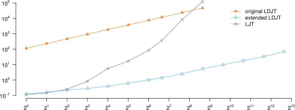
Figure 5: Y-axis: runtimes [seconds], x-axis: maximum time steps, both in log scale

7 Evaluation

For the evaluation, we use the example model $G^{ex}$ with the set of evidence being empty, for $|\mathcal{D}(X)|=10$, $|\mathcal{D}(P)|=3$, $|\mathcal{D}(C)|=20$, and the queries $\{Hot_{t},AttC_{t}(c_{1}),DoR_{t}(x_{1})\}$ for each time step. We compare the runtimes on commodity hardware with 16 GB of RAM of the extended LDJT version against LDJT’s original version and then also against LJT for multiple maximum time steps.

Figure 5 shows the runtime in seconds for each maximum time step. We can see that the runtime of the extended LDJT (diamond) and the original LDJT (filled triangle) is, as expected, linear, while the runtime of LJT (cross) roughly is exponential, to answer queries for changing maximum number of time steps. Further, we can see how crucial preventing groundings is. Due to the FO jtree construction overhead, the extended version is about a magnitude of three faster for first few time steps, but the construction overhead becomes negligible with more time steps. Overall, the extended LDJT is up to a magnitude of four faster.

Additionally, we see the runtimes of LJT. The runtimes with and without fusion are about the same and thus not distinguished. LJT is faster for the initial time steps, especially in case grounding are prevented by unrolling. Nonetheless, after several time steps, the size of the parclusters becomes a big factor, which also explains the exponential behaviour (?). To summarise the evaluation results, on the one hand, we see how crucial the prevention of groundings is and, on the other hand, how crucial the dedicated handling of temporal aspects is.

8 Conclusion

We present how LDJT can prevent unnecessary groundings by delaying eliminations to the next time step and thereby changing the elimination order. To delay eliminations, LDJT increases the in-cluster of the temporal FO jtree structure and the separator between out-cluster and in-cluster with PRVs, which lead to the groundings. Further, due to temporal m-separation, which is ensured by the in- and out-clusters, LDJT reuses the same changed FO jtree structure for all time steps $t>0$. First results show that the extended LDJT significantly outperforms the orignal version and LJT if unnecessary groundings occur.

We currently work on extending LDJT to also calculate the most probable explanation. Other interesting future work includes a tailored automatic learning for PDMs, parallelisation of LJT, and improved evidence entering.

References

- [Ahmadi et al. 2013] Ahmadi, B.; Kersting, K.; Mladenov, M.; and Natarajan, S. 2013. Exploiting Symmetries for Scaling Loopy Belief Propagation and Relational Training. Machine learning 92(1):91–132.
- [Braun and Möller 2016] Braun, T., and Möller, R. 2016. Lifted Junction Tree Algorithm. In Proceedings of the Joint German/Austrian Conference on Artificial Intelligence (Künstliche Intelligenz), 30–42. Springer.
- [Braun and Möller 2017] Braun, T., and Möller, R. 2017. Preventing Groundings and Handling Evidence in the Lifted Junction Tree Algorithm. In Proceedings of the Joint German/Austrian Conference on Artificial Intelligence (Künstliche Intelligenz), 85–98. Springer.
- [Braun and Möller 2018] Braun, T., and Möller, R. 2018. Counting and Conjunctive Queries in the Lifted Junction Tree Algorithm. In Postproceedings of the 5th International Workshop on Graph Structures for Knowledge Representation and Reasoning, GKR 2017, Melbourne, Australia, August 21, 2017. Springer.
- [Darwiche 2009] Darwiche, A. 2009. Modeling and Reasoning with Bayesian Networks. Cambridge University Press.
- [de Salvo Braz 2007] de Salvo Braz, R. 2007. Lifted First-Order Probabilistic Inference. Ph.D. Dissertation, Ph. D. Dissertation, University of Illinois at Urbana Champaign.
- [Dignös, Böhlen, and Gamper 2012] Dignös, A.; Böhlen, M. H.; and Gamper, J. 2012. Temporal Alignment. In Proceedings of the 2012 ACM SIGMOD International Conference on Management of Data, 433–444. ACM.
- [Dylla, Miliaraki, and Theobald 2013] Dylla, M.; Miliaraki, I.; and Theobald, M. 2013. A Temporal-Probabilistic Database Model for Information Extraction. Proceedings of the VLDB Endowment 6(14):1810–1821.
- [Gehrke, Braun, and Möller 2018] Gehrke, M.; Braun, T.; and Möller, R. 2018. Lifted Dynamic Junction Tree Algorithm. In Proceedings of the 23rd International Conference on Conceptual Structures. Springer. [to appear].
- [Geier and Biundo 2011] Geier, T., and Biundo, S. 2011. Approximate Online Inference for Dynamic Markov Logic Networks. In Proceedings of the 23rd IEEE International Conference on Tools with Artificial Intelligence (ICTAI), 764–768. IEEE.
- [Lauritzen and Spiegelhalter 1988] Lauritzen, S. L., and Spiegelhalter, D. J. 1988. Local Computations with Probabilities on Graphical Structures and their Application to Expert Systems. Journal of the Royal Statistical Society. Series B (Methodological) 157–224.
- [Manfredotti 2009] Manfredotti, C. E. 2009. Modeling and Inference with Relational Dynamic Bayesian Networks. Ph.D. Dissertation, Ph. D. Dissertation, University of Milano-Bicocca.
- [Milch et al. 2008] Milch, B.; Zettlemoyer, L. S.; Kersting, K.; Haimes, M.; and Kaelbling, L. P. 2008. Lifted Probabilistic Inference with Counting Formulas. In Proceedings of AAAI, volume 8, 1062–1068.
- [Murphy and Weiss 2001] Murphy, K., and Weiss, Y. 2001. The Factored Frontier Algorithm for Approximate Inference in DBNs. In Proceedings of the Seventeenth conference on Uncertainty in artificial intelligence, 378–385. Morgan Kaufmann Publishers Inc.
- [Murphy 2002] Murphy, K. P. 2002. Dynamic Bayesian Networks: Representation, Inference and Learning. Ph.D. Dissertation, University of California, Berkeley.
- [Nitti, De Laet, and De Raedt 2013] Nitti, D.; De Laet, T.; and De Raedt, L. 2013. A particle Filter for Hybrid Relational Domains. In Proceedings of the IEEE/RSJ International Conference on Intelligent Robots and Systems (IROS), 2764–2771. IEEE.
- [Papai, Kautz, and Stefankovic 2012] Papai, T.; Kautz, H.; and Stefankovic, D. 2012. Slice Normalized Dynamic Markov Logic Networks. In Proceedings of the Advances in Neural Information Processing Systems, 1907–1915.
- [Poole 2003] Poole, D. 2003. First-order probabilistic inference. In Proceedings of IJCAI, volume 3, 985–991.
- [Richardson and Domingos 2006] Richardson, M., and Domingos, P. 2006. Markov Logic Networks. Machine learning 62(1):107–136.
- [Taghipour et al. 2013] Taghipour, N.; Fierens, D.; Davis, J.; and Blockeel, H. 2013. Lifted Variable Elimination: Decoupling the Operators from the Constraint Language. Journal of Artificial Intelligence Research 47(1):393–439.
- [Taghipour, Davis, and Blockeel 2013] Taghipour, N.; Davis, J.; and Blockeel, H. 2013. First-order Decomposition Trees. In Proceedings of the Advances in Neural Information Processing Systems, 1052–1060.
- [Thon, Landwehr, and De Raedt 2011] Thon, I.; Landwehr, N.; and De Raedt, L. 2011. Stochastic relational processes: Efficient inference and applications. Machine Learning 82(2):239–272.
- [Vlasselaer et al. 2014] Vlasselaer, J.; Meert, W.; Van den Broeck, G.; and De Raedt, L. 2014. Efficient Probabilistic Inference for Dynamic Relational Models. In Proceedings of the 13th AAAI Conference on Statistical Relational AI, AAAIWS’14-13, 131–132. AAAI Press.
- [Vlasselaer et al. 2016] Vlasselaer, J.; Van den Broeck, G.; Kimmig, A.; Meert, W.; and De Raedt, L. 2016. TP-Compilation for Inference in Probabilistic Logic Programs. International Journal of Approximate Reasoning 78:15–32.