Abstract

We apply techniques in natural language processing, computational linguistics, and machine-learning to investigate papers in hep-th and four related sections of the arXiv: hep-ph, hep-lat, gr-qc, and math-ph. All of the titles of papers in each of these sections, from the inception of the arXiv until the end of 2017, are extracted and treated as a corpus which we use to train the neural network Word2Vec. A comparative study of common $n$-grams, linear syntactical identities, word cloud and word similarities is carried out. We find notable scientific and sociological differences between the fields. In conjunction with support vector machines, we also show that the syntactic structure of the titles in different subfields of high energy and mathematical physics are sufficiently different that a neural network can perform a binary classification of formal versus phenomenological sections with 87.1% accuracy, and can perform a finer five-fold classification across all sections with 65.1% accuracy.

1 Introduction and Summary

The arXiv [1], introduced by Paul Ginsparg to communicate preprints in high energy theoretical physics in 1991 and democratize science [2], has since expanded to encompass areas of physics, mathematics, computer science, quantitative biology, quantitative finance, statistics, electrical engineering and systems science, and economics and now hosts nearly $1.4$ million preprints. In comparison with $123,523$ preprints archived and distributed in 2017 [3], around $2.4$ million scholarly articles across all fields of academic enquiry are published every year [4]. As a practitioner in science, keeping up with the literature in order to invent new knowledge from old is itself a formidable labour that technology may simplify.

In this paper, we apply the latest methods in computational linguistics, natural language processing and machine learning to preprints in high energy theoretical physics and mathematical physics to demonstrate important proofs of concept: by mapping words to vectors, algorithms can automatically sort preprints into their appropriate disciplines with over 65% accuracy, and these vectors capture the relationships between scientific concepts. In due course, many interesting properties of the word-vectors emerge and we make comparative studies across the different sub-fields. Developing this technology will facilitate the use of computers as idea generating machines [5]. This is complementary to the role of computers in mathematics as proof assistants [6] and problem solvers [7].

The zeitgeist of the moment has seen computers envelop our scientific lives. In particular, in the last few years, we have seen an explosion of activity in applying artificial intelligence to various aspects of theoretical physics (cf. [8] for a growing repository of papers). In high energy theoretical physics, there have been attempts to understand the string landscape using deep neural networks [9], with genetic algorithms [10], with network theory [11, 12], for computing Calabi–Yau volumes [13], for F-theory [14], and for CICY manifolds [15] etc.

Inspired by a recent effort by Evert van Nieuwenburg [16] to study the language of condensed matter theory, we are naturally led to wonder what the latest technology in language-processing using machine learning, utilized by the likes of Google and Facebook, would tell us about the language of theoretical physics.

As members of the high energy theoretical physics community, we focus on particular fields related to our own expertise: hep-th (high energy physics — theory), hep-ph (high energy physics — phenomenology), hep-lat (high energy physics — lattice), gr-qc (general relativity and quantum cosmology), and math-ph (mathematical physics). In December 2017, we downloaded the titles and abstracts of the preprints thus far posted to arXiv in these disciplines. In total, we analyze a collection of some $395,000$ preprints. Upon cleaning the data, we use Word2vec [17, 18] to map the words that appear in this corpus of text to vectors in $\mathbb{R}^{400}$. We then proceed to investigate this using the standard Python package gensim [19]. In parallel, a comparative study of the linguistic structure of the titles in the different fields in carried out.

It should be noted that there have been investigations of the arXiv using textual analyses [20, 21, 22]. In this paper, we focus on the five sections of theory/phenomenology in the high-energy/mathematical physics community as well as their comparisons with titles outside of academia. Moreover, we will focus on the syntactical identities which are generated from the contextual studies. Finally, where possible we attempt to provide explanations why certain features in the data emerge, features which are indicative of the socio-scientific nature of the various sub-disciplines of the community.

We hope this paper will have readers in two widely-separated fields: our colleagues in the high energy theory community and those who study natural language processing in academia or in industry. As such, some guidance to the structure of what follows is warranted. For physicists, the introductory material in Section 2 will serve as a very brief summary and introduction to the vocabulary and techniques of computational textual analysis. Experts in this area can skip this entirely. Section 3 begins in Section 3.1 with an introduction to the five arXiv sections we will be studying. Our colleagues in physics will know this well and may skip this. Data scientists will want to understand our methods for preparing the data for analysis, which is described in Section 3.2, followed by some general descriptive properties of the hep-th vocabulary in Section 3.3. The analysis of hep-th using the results of Word2vec’s neural network are presented in Section 4, and those of the other four arXiv sections in Section 5. These two sections will be of greatest interest and amusement for authors who regularly contribute to the arXiv, but we would direct data scientists to Section 4.1, in which the peculiar geometrical properties of our vector space word embedding are studied, in a manner similar to that of the recent work by Mimno and Thompson [24]. Our work culminates with a demonstration of the power of Word2vec, coupled with a support vector machine classifier, to accurately sort arXiv titles into the appropriate sub-categories. We summarize our results, and speculate about future directions in Section 7.

2 Computational Textual Analysis

2.1 Distributed Representation of Words

We begin by reviewing some terminology and definitions (the reader is referred to [25, 26] for more pedagogical material). A dictionary is a finite set whose elements are words, each of which is an ordered finite sequence of letters. An $n$-gram is an ordered sequence of $n$ words. A sentence can be considered an $n$-gram. Moreover, since we will not worry about punctuation, we shall use these two concepts interchangeably. Continuing in a familiar manner, an ordered collection of sentences is a document and a collection (ordered if necessary) of documents is a corpus:

$$\mbox{word}\in\mbox{$n$-gram}\subset\mbox{document}\subset\mbox{corpus}\ .$$ (1)

Note that for our purposes the smallest unit is “word” rather than “letters” and we will also not make many distinctions among the three set inclusions, i.e., after all, we can string the entire corpus of documents into a single $n$-gram for some very large $n$. As we shall be studying abstracts and titles of scientific papers, $n$ will typically be no more than $\mathcal{O}(10)$ for titles, and $\mathcal{O}(100)$ for abstracts.

In order to perform any analysis, one needs a numerical representation of words and $n$-grams; this representation is often called a word embedding. Suppose we have a dictionary of $N$ words. We can lexicographically order them, for instance, giving us a natural vector of length $N$. Each word is a vector containing precisely a single $1$, corresponding to its position in the dictionary and $0$ everywhere else. The entire dictionary is thus the $N\times N$ identity matrix and the $i$-th word is simply the elementary basis vector $e_{i}$. This representation is sometimes called the one-hot form of a vector representation of words (the hot being the single $1$-entry). This representation of words is not particularly powerful because not much more than equality-testing can be performed.

The insight of [27] is to have a weighted vectorial representation $\vec{v_{w}}$, constructed so as to reflect the meaning of the word $w$. For instance, $\vec{v}_{\mbox{``car''}}-\vec{v}_{\mbox{``cars''}}$ should give a close value to $\vec{v}_{\mbox{``apple''}}-\vec{v}_{\mbox{``apples''}}$. Note that, for the sake of brevity, we will be rather lax about the notation on words: i.e., $\vec{v}_{\mbox{``word''}}$ and “word” will be used interchangeably. Indeed, we wish to take advantage of the algebraic structure of a vector space over $\mathbb{R}$ to allow for addition and subtraction of vectors. An archetypal example in the literature is that

$$\mbox{``king''}-\mbox{``man''}+\mbox{``woman''}=\mbox{``queen''}\ .$$ (2)

In order to arrive at a result such as (2), we need a few non-trivial definitions.

Definition 1.

A context window with respect to a word $W$, or specifically, a $k$-around context window with respect to $W$, is a subsequence within a sentence or $n$-gram containing the word $W$, containing all words a distance $k$ away from $W$, in both directions. Similarly, a $k$ context window, without reference to a specific word, is simply a subsequence of length $k$.

For example, consider the following $46$-gram, taken from the abstract of [28], which is one of the first papers to appear on hep-th in 1991:

String theories with two dimensional space-time target spaces are characterized by the existence of a ground ring of operators of spin (0,0). By understanding this ring, one can understand the symmetries of the theory and illuminate the relation of the critical string theory to matrix models.

In this case, a $2$-around context window for the word “spaces” is the 5-gram “space-time target spaces are characterized”. Meanwhile, $2$-context windows are $2$-grams such as “ground ring” or “(0,0)”. Note that we have considered hyphenated words as a single word, and that the $n$-gram has crossed between two sentences.

The above example immediately reveals one distinction of scientific and mathematical writing that does not often appear in other forms of writing: the presence of mathematical symbols and expressions in otherwise ordinary prose. Our procedure will be to ignore all punctuation marks in the titles and abstracts. Thus, “(0,0)” becomes the ‘word’ “00”. Fortunately, such mathematical symbols are generally rare in the abstracts of papers (though, of course, they are quite common the body of the works themselves), and even more uncommon in the titles of papers.

The correlation between words in the sense of context, reflecting their likely proximity in a document, can be captured by a matrix:

Definition 2.

The $k$ co-occurrence matrix for an $n$-gram is a symmetric, $0$-diagonal square matrix (of dimension equalling the number of unique words) which encodes the adjacency of the words within a $k$ context window.

Continuing with the above example of the $46$-gram, we list all the unique words horizontally and vertically, giving a $37\times 37$ matrix for this sentence (of course, one could consider the entire corpus as a single $n$-gram and construct a much larger matrix). The words can be ordered lexicographically, {“a”, “and”, “are”, …}. One can check that in a $2$-context-window (testing whether two words are immediate neighbors), for instance, “a” and “and” are never adjacent; thus, the $(i,j)=(1,2)$ entry of the $2$ co-occurrence matrix is $0$.

2.2 Neural Networks

The subject of neural networks is vast and into its full introduction we certainly shall not delve. Since this section is aimed primarily at theoretical physicists and mathematicians, it is expedient only to remind the reader of the most rudimentary definitions, enough to prepare for the ensuing subsection. We recall first that:

Definition 3.

A neuron is a (typically analytic) function $f(\sum_{i=1}^{k}w_{i}\cdot x_{i}+b)$ whose argument $x_{i}$ is the input, typically some real tensor with multi-index $i$. The value of $f$ is called the output, the parameter $w_{i}$ is some real tensor called weights with $\cdot$ appropriate contraction of the indices and the parameter $b\in\mathbb{R}$ is called the off-set or bias.

The function $f$ is called an activation function and often takes the non-linear forms of a hyperbolic tangent or a sigmoid. The parametres $w_{i}$ and $b$ are to be determined empirically as follows:

• Let there be a set of input values $x_{i}^{j}$ labelled by $j=1,\ldots,T$ such that the output $y^{j}$ is known: $\{x_{i}^{j},y^{j}\}$ is called the training set;

• Define an appropriate measure of goodness-of-fit, typically one uses the standard deviation (mean-square-error)
  

  $$Z(w_{i},b):=\sum\limits_{j=1}^{T}\big{(}f(\sum_{i=1}^{k}w_{i}\cdot x_{i}^{j}+b)-y^{j}\big{)}^{2}\ ;$$

• Minimize $Z(w_{i},b)$ as a function of the parameters (often numerically by steepest descent methods), whereby determining the parameters $(w_{i},b)$;

• Test the now-fixed neuron on unseen input data.

At this level, we are doing no more than (non-linear) regression by best-fit. We remark that in the above definition, we have made $f$ a real-valued function for simplicity. In general, $f$ will be itself tensor-valued.

The power of the neural network comes from establishing a network structure of neurons — much like the complexity of the brain comes from the myriad inter-connectivities among biological neurons:

Definition 4.

A neural network is a finite directed graph, with possible cycles, each node of which is a neuron, such that the input for the neuron at tail of an arrow is the output of the neuron at the head of the arrow. We organize the neural network into layers so that

1. The collection of nodes with arguments explicitly involving the actual input data is called the input layer;

2. Likewise, the collection of nodes with arguments explicitly involving the actual output of data is called the output layer;

3. The collection of all other nodes are called hidden layers.

Training the neural network proceeds as the algorithm above, with the input and output layers interacting with the training data and each neuron giving its own set of weight/off-set parameters. The measure $Z$ will thus be a function in many variables over which we optimize.

One might imagine the design of a neural network – with its many possible hidden layers, neuron types, and internal architecture – would be a complicated affair, and highly-dependent on the problem at hand. But in this we can take advantage of the powerful theorem by Cybenko and Hornik [29]:

Theorem 1.

Universal Approximation Theorem [Cybenko-Hornik] A neural network with a single hidden layer with a finite number of neurons can approximate any neural network in the sense of prescribing a dense set within the set of continuous functions on $\mathbb{R}^{n}$.

2.3 Word2Vec

We now combine the concepts in the previous two subsections to use a neural network to establish a predictive embedding of words. In particular, we will be dealing with Word2Vec [27], which has emerged as one of the most sophisticated models for natural language processing (NLP). The Word2Vec software can utilize one of two related neural network models: (1) the continuous bag of words [CBOW] model, or (2) the skip-gram [SG] model, both consisting of only a single hidden layer, which we will shortly define below in detail.

The CBOW approach is perhaps the most straight-forward: given an $n$-gram, form the multiset (‘bag’) of all words found in the $n$-gram, retaining multiplicity information. One might also consider including the set of all $m$-grams ($m\leq n$) in the multiset. A collection of such ‘bags’, all associated with a certain classifier (say, ‘titles of hep-th papers’), then becomes the input upon which the neural network trains.

The SG model attempts to retain contextual information by utilizing context windows in the form of $k$-skip-$n$-grams, which are $n$ grams in which each of the components of the $n$-gram occur at a distance $k$ from one another. That is, length-$k$ gaps exist in the $n$-grams extracted from a piece of text. The fundamental object of study is thus a $k$-skip-$n$-gram, together with the set of elided words. It is the collection of these objects that becomes the input upon which the neural network trains.

The two neural network approaches are complementary to one another. Coarsely speaking, CBOW is trained to predict a word given context, while SG is trained to predict context given a word. To be more concrete, a CBOW model develops a vector space of word embeddings in such a way as to maximize the likelihood that, given a collection of words, it will return a single word that best matches the context of the collection. By contrast, the vector space of word embeddings constructed by the SG model is best suited to give a collection of words likely to be found in context with a particular word.

While CBOW and SG have specific roles, the default method for generating word embeddings in a large corpus is to use the CBOW model. This is because it is clearly more deterministic to have more input than output, i.e., a single-valued function is easier to handle than a multi-valued one. This will be our choice going forward. Note that our ultimate interest is in the information contained in the word embedding itself, and not in the ability of the model to make predictions on particular words. When we attack the document classification problem via machine learning, in Section 6, we will use the distributed representation generated by Word2Vec as training data for a simple support vector machine classifier.

With the CBOW model in mind, therefore, let us consider the structure of the underlying neural network, depicted schematically in Figure 1. Let $V$ denote the vocabulary size so that any word can be ab initio trivially represented by a one-hot vector in $\mathbb{R}^{V}$. The dimension $V$ could be rather large, and we will see how a reduction to an $N$-dimensional representation is achieved. The overall structure has three layers:

1. The input layer is a list of $C$ context words. Thus, this is a list of $C$ vectors $\vec{x}_{c=1,\ldots,C}$ each of dimension $V$. We denote these component-wise as $x_{c=1,\ldots,C}^{i=1,\ldots,V}$. This list is the “bag of words” of CBOW, and in our case each such list will represent a single, contextually-closed object, such as a paper title or paper abstract.

2. The output layer is a single vector $\vec{y}$ of dimension $V$. We will train the neural network with a large number of examples where $y$ is known, given the words $\vec{x}$ within a context $C$, so that one could thence predict the output. Continuing with our example of [28], the title of this paper provides a specific context $C$: “Ground ring of two-dimensional string theory”. Thus for an input of {“ring”, “of”, “string”, “theory”}, we ideally wish to return the vector associated with “two-dimensional” when the window size is set to two. Of course, we expect words like “theory” to appear in many other titles. The neural network will therefore optimize over many such titles (contexts) to give the “best” vector representation of words.

3. There is a single hidden layer consisting of $N$ neural nodes. The function from the input layer to the hidden layer is taken to be linear map, i.e., a $V\times N$ matrix $W_{1}$ of weights. Likewise, the map from the hidden layer to the output layer is an $N\times V$ weight matrix $W_{2}$. Thus, in total, we have $2V\times N$ weights which will be optimized by training. Note that $N$ is a fixed parameter (or hyper-parameter) and is a choice. Typically, $N\sim 300-500$ has been shown to be a good range [25, 26, 30]; in this paper we take $N=400$.

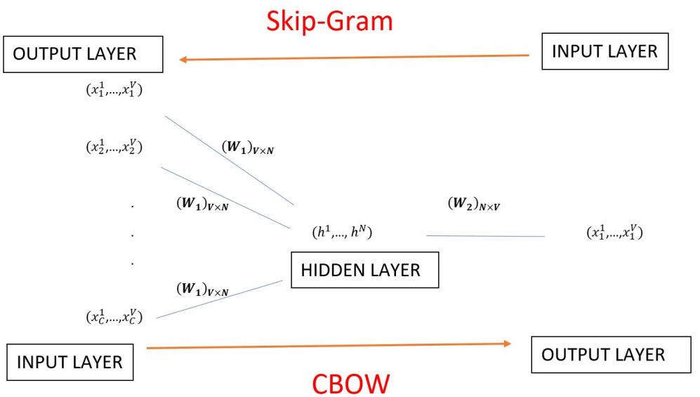
Figure 1: The neural network consists of a single hidden layer, which constructs a mapping from $\mathbb{R}^{V}$ to $\mathbb{R}^{V}$. The parameters to be fit by the neural network are the transformation matrices $W_{1}$ and $W_{2}$, with the entries of $W_{1}$ constituting the word embedding into the space $\mathbb{R}^{N}$. After training, a CBOW model takes multiple $\vec{x}$ inputs, associated with a particular context $C$, and maps them to a single output vector. Conversely, after training, a SG model takes a single word $\vec{x}$ as an input, and returns the set of vectors $\vec{x}_{C}$ associated with the appropriate context.

To find the optimal word embedding, or most faithful representation of the words in $\mathbb{R}^{N}$, each input vector $\vec{x}_{c}$, in a particular context (or bag), is mapped by $W_{1}$ to an $N$ vector (the actual word-vector after the neural network is trained) $\vec{h}=[\vec{x}_{c}]^{T}\cdot W_{1}$. Of course, because $\vec{x}$ is a Kronecker-delta, $\vec{h}$ is just the $k$-th row of $W_{1}$ where $k$ is the only component equal to $1$ in $\vec{x}_{c}$. A measure of the proximity between an input and output word-vector is the weighted inner product

$$\left<\vec{x}_{c},\ \vec{y}\right>:=[\vec{x}_{c}]^{T}\cdot W_{1}\cdot W_{2}\cdot\vec{y}\,.$$ (3)

Hence, for each given context $C_{\alpha}$, where $\alpha$ might label contextually-distinct objects (such as paper titles) in our training set, we can define a score for each component $i$ (thus in the one-hot representation, each word) $u_{c}^{j=1,\ldots,V}$ in the vocabulary as

$$u^{j}_{c}:=[\vec{x}_{c}]^{T}\cdot W_{1}\cdot W_{2}\,.$$ (4)

As always with a list, one can convert this to a probability (for each $c$ and each component $j$) via the softmax function:

$$p(u^{j}_{c}|x_{c}):=\frac{\exp(u^{j}_{c})}{\sum\limits_{j=1}^{V}\exp(u^{j}_{c})}\,.$$ (5)

Finally, the components of the output vector $\vec{y}$ is the product over the context words of these probabilities

$$y^{j}=\prod\limits_{c=1}^{C}\frac{\exp(u^{j}_{c})}{\sum\limits_{j=1}^{V}\exp(u^{j}_{c})}\,.$$ (6)

The neural network is trained by maximizing the log-likelihood of the probabilities across all of our training contexts

$$Z(W_{1},W_{2}):=\frac{1}{|D|}\sum\limits_{\alpha=1}^{|D|}\log\prod\limits_{c=1}^{C_{\alpha}}\frac{\exp([\vec{x}_{c}]^{T}\cdot W_{1}\cdot W_{2})}{\sum\limits_{j=1}^{V}\exp([\vec{x}_{c}]^{T}\cdot W_{1}\cdot W_{2})}\,,$$ (7)

where we have written the functional dependence in terms of the $2V\times N$ variables of $W_{1}$ and $W_{2}$ because we need to extremize over these. In (7), the symbol $|D|$ represents the number of independent contexts in the training set (i.e., $\alpha=1,\dots,|D|$).

We will perform a vector embedding study as discussed above, and perform various contextual analyses using the bag-of-words model. Fortunately, many of the the requisite algorithms have been implemented into python with the gensim package [19].

2.4 Distance Measures

Once we have represented all words in a corpus as vectors in $\mathbb{R}^{N}$, we will loosely use the “$=$” sign to denote that two words are “close” in the sense that the Euclidean distance between the two vectors is small. In practice, this is measured by computing the cosine of the angle between the vectors representing the words. That is, given words $w_{1}$ and $w_{2}$, and their associated word vectors $\vec{v}_{w_{1}}$ and $\vec{v}_{w_{2}}$, we can define distance as

$$d(w_{1},w_{2}):=\frac{\vec{v}_{w_{1}}\cdot\vec{v}_{w_{2}}}{\left|\vec{v}_{w_{1}}\right|\left|\vec{v}_{w_{2}}\right|}\ .$$ (8)

Generically, we expect $d(w_{1},w_{2})$ will be close to zero, meaning that two words are not related. However, if $d(w_{1},w_{2})$ is close to $+1$, the words are similar. Indeed, for the same word $w$, tautologically $d(w,w)=1$. If $d(w_{1},w_{2})$ is close to $-1$, then the words are dissimilar in the sense that they tend to be far apart in any context window. We will adopt, for clarity, the following notation:

Definition 5.

Two words $w_{1}$ and $w_{2}$ are

similar

in the sense of $d(w_{1},w_{2})\sim 1$ (including the trivial case of equality), and are denoted as $w_{1}=w_{2}$; and

dissimilar

in the sense of $d(w_{1},w_{2})\sim-1$, and are denoted as $w_{1}\neq w_{2}$.

Vector addition generates signed relations such as $w_{1}+w_{2}=w_{3}$, $w_{1}+w_{2}-w_{3}=w_{4}$, etc. We will call these relations linear syntactic identities.

For instance, our earlier example of (2) is one such identity involving four words. Henceforth, we will bear in mind that “=” denotes the closest word within context windows inside the corpus. Finding such identities in the hep-th arXiv and its sister repositories will be one of the goals of our investigation.

As a technical point, it should be noted that word-vectors do not span a vector space $V$ in the proper sense. First, there is no real sense of closure, one cannot guarantee the sum of vectors is still in $V$, only the closest to it by distance. Second, there is no sense of scaling by elements of the ground field, here $\mathbb{R}$. In other words, though the components of word-vectors are real numbers, it is not clear what $aw_{1}+bw_{2}$ for arbitrary $a,b\in\mathbb{R}$ means. The only operation we can perform is the one discussed above by adding two and subtracting two vectors in the sense of a syntactic identity.

2.5 Term Frequency and Document Frequency

Following our model of treating the set of titles/abstracts of each section as a single document, one could thus consider the arXiv as a corpus. The standard method of cross-documentary comparisons is the so-called term-frequency - inverse document frequency (tf-idf), which attempts to quantify the importance of a particular word in the corpus overall:

Definition 6.

Let $D$ be a corpus of documents, $d\in D$ a document and $t\in d$ be a word (sometimes also called a term) in $d$. Let $f(t,d):=|x\in d:x=t|$ represent the raw count of the number of appearances of the word $t$ in the document $d$, where the notation $|X|$ means the cardinality of the set represented by $X$.

• The term frequency $\mathop{\rm tf}(t,d)$ is a choice of function of the count of occurrences $f(t,d):=|x\in d:x=t|$ of $t$ in $d$;

• The inverse document frequency $\mathop{\rm idf}(t,D)$ is the minus logarithm of the fraction of documents containing $t$:

  $$\mathop{\rm idf}(t,D):=-\log\frac{|d\in D:t\in d|}{|D|}=\log\frac{|D|}{|d\in D:t\in d|}\ ;$$

• The tf-idf is the product of the above two: $\mathop{\rm tfidf}(t,d,D):=\mathop{\rm tf}(t,d)\cdot\mathop{\rm idf}(t,D)$  .

In the context of our discussion in Section 2.3, $D$ might represent the sum of all titles, and each $d$ might represent a distinct title (or “context”).

The simplest $\mathop{\rm tf}$ is, of course, to just take $f(t,d)$ itself. Another commonly employed $\mathop{\rm tf}$ is a logarithmically scaled frequency $\mathop{\rm tf}(t,d)=\log(1+f(t,d))$, which we shall utilize in our analysis. Thus we will have

$$\mathop{\rm tfidf}(t,d,D)=\log(1+|x\in d:x=t|)\log\frac{|D|}{|d\in D:t\in d|}\in\mathbb{R}_{\geq 0}\,,$$ (9)

where $d$ might represent the string of words in all titles in a given arXiv section, labeled by $D$. The concept of weighting by the inverse document frequency is to penalize those words which appear in virtually all documents. Thus a tf-idf score of zero means that the word either does not appear at all in a document, or it appears in all documents.

3 Data Preparation

3.1 Data Sets

As mentioned in the introduction, we will be concerned primarily with the language of hep-th, but we will be comparing this section of the arXiv with closely-related sections. The five categories that will be of greatest interest to us will be:

hep-th

Begun in the summer of 1991, hep-th was the original preprint listserv for theoretical physics. Traditionally the content has focused on formal theory, including (but not limited to), formal results in supersymmetric field theory, string theory and string model building, and conformal field theory.

hep-ph

Established in March of 1992, hep-ph was the bulletin board designed to host papers in phenomenology – a term used in high energy theory to refer to model-building, constraining known models with experimental data, and theoretical simulation of current or planned particle physics experiments.

hep-lat

Launched in April of 1992, hep-lat is the arXiv section dedicated to numerical calculations of quantum field theory observables using a discretization of space-time (“lattice”) that allows for direct computation of correlation functions that cannot be computed by standard perturbative (Feynman diagram) techniques. While closely related to the topics studied by authors in hep-th and hep-ph, scientists posting research to hep-lat tend to be highly-specialized, and tend to utilize high performance computing to perform their calculations at a level that is uncommon in the other arXiv sections.

gr-qc

The bulletin board for general relativity and quantum cosmology, gr-qc, was established in July of 1992. Publications submitted to this section of arXiv tend to involve topics such as black hole solutions to general relativity in various dimensions, treatment of spacetime singularities, information theory in general relativity, and early universe physics. Explicit models of inflation, and their experimental consequences, may appear in gr-qc, as well as in hep-th and (to a lesser extent) hep-ph. Preprints exploring non-string theory approaches to quantum gravity typically appear here.

math-ph

The youngest of the sections we consider, math-ph was born in March of 1998 by re-purposing a section of the general physics arXiv then called “Mathematical Methods in Physics”. As the original notification email advised, “If you are not sure whether or not your submission is physics, then it should be sent to math-ph.” Today, papers submitted to math-ph are typically the work of mathematicians, whose intended audience is other mathematicians, but the content of which tends to be of relevance to certain areas of string theory and formal gauge theory research.

Given that part of the motivation for the current work is to use language as a marker for understanding the social dynamics – and overlapping interests – of our community, it is relevant to mention a few important facts about the evolution of the arXiv. The arXiv repository began originally as a listserv, which sent daily lists of titles and abstracts of preprints to its subscribers. The more technically savvy of these recipients could then seek to obtain these preprints via anonymous ftp or gopher. A true web-interface arrived at the end of 1993.

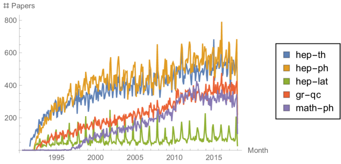
Figure 2: Number of papers published for five related sections of high energy physics, since the beginning of the arXiv in 1991, until the end of December, 2017.

New sections of the arXiv proliferated rapidly in the early 90’s, at the request of practicing physicists. Given the limited bandwith – both literal and metaphorical – of most university professors, it seemed optimal to sub-divide the arXiv into ever smaller and more focused units. Thus, research was pigeonholed into “silos” by design. As a result, individual faculty often came to identify strongly with the section of arXiv to which they regularly posted. While cross-listing from a primary section to a secondary (and even a tertiary) section began in May of 1992, such cross-listing was generally rare throughout much of the early years of the arXiv. The total number of publications per month, in these five sections of arXiv, is shown in Figure 2. The reader is also referred to arXiv itself for a detailed analysis of such statistics.

arXiv	No. of	Titles		Abstracts
Section	Papers	Mean Length	Unique Words	Mean Length	Unique Words
hep-th	120,249	8.29	37,550	111.2	276,361
hep-ph	133,346	9.34	46,011	113.4	349,859
hep-lat	21,123	9.31	10,639	105.7	78,175
gr-qc	69,386	8.74	26,222	124.4	194,368
math-ph	51,747	9.19	28,559	106.1	194,149

Table 1: Gross properties of the five arXiv sections studied in this paper. Numbers includes all papers through the end of 2017. The count of unique words does not distinguish upper and lower-case forms of a word. “Length” here means the number of words in a given title or in a given sentence in the abstract. As anticipated, there is remarkable similarity across these five sections of arXiv for the mean lengths.

We extracted metadata from the arXiv website, in the form of titles and abstracts for all submissions, using techniques described in [16]. The number of publications represented by this dataset is given in Table 1. Also given is the mean number of words in the typical title and abstract of publications in each of the five sections, as well as the count of unique words in each of the sections.

Titles and abstracts are, of course, different categories serving different functions. To take a very obvious example, titles do not necessarily need to obey the grammatical rules which govern standard prose. Nevertheless, we can consider each title in hep-th, or any other section of the arXiv, as a sentence. For hep-th this gives us the raw data of $120,249$ sentences.

Abstracts are inherently different. They represent a collection of sentences which cluster around particular semantic content. Grammatically, they are quite different from the titles. As an example, being comprised of full sentences suggests that punctuation is meaningful in the abstract, while generally irrelevant in titles. Finally, whereas each of the 120,249 titles in hep-th can be though of as semantically distinct sentences in a single document (the entirety of hep-th), the abstracts must be thought of as individual documents within a larger corpus. This notion of “grouping” sentences into semantic units can make the word embedding process more difficult.

While variants of Word2Vec exist which can take this nuance into account, we will simply aggregate all abstracts on each section of the arXiv, then separate them only by full sentences. For hep-th, the abstracts produce 608,000 sentences over all 120,249 papers, comprising 13,347,051 words, of which 276,361 are unique.

3.2 Data Cleaning: Raw, Processed and Cleaned

As any practicing data scientist will attest, cleaning and pre-processing raw data is a crucial step in any analysis in which machine learning is to be utilized. The current data set is no exception. Indeed, some data preparation issues in this paper are likely to be unique in the natural language processing literature. In this subsection we describe the steps we took to prepare the data for neural network analysis.

Our procedure for pre-processing data proceeded along the following order of operations:

1. Put everything into lower case;

2. Convert all key words, typically nouns, to singular case. Indeed, it typically does not make sense to consider the words “equation” and “equations” as different concepts;

3. Spellings of non-English names, including LaTeX  commands, are converted to standard English spelling. For example, “schroedinger”, “schr\"odinger” and “schr"odinger” will all be replaced by simply “schrodinger” (note that at this stage we already do not have any further upper case letters so the “s” is not capitalized);

4. At this stage, we can replace punctuation such as periods, commas, colons, etc, as well as LaTeX backslash commands such as \c{} which do appear (though not often) in borrowed words such as “aperçu”, as well as \cal for calligraphic symbols (which do appear rather often), such as in “${\cal N}=4$ susy”. Note that we keep parentheses intact because words such as su(n) appear often; so too we will keep such LaTeX commands as ^ and _ because superscripts and subscripts, when they appear in a title, are significant;

5. Now, we reach a highly non-trivial part of the replacements: including important technical acronyms. Though rarely used directly in titles, acronyms are common in our field. All acronyms serve the purpose of converting an $n$-gram into a single monogram. So, for example, “quantum field theory” should appear together as a single unit, to be replaced by “qft”. This is a special case of bi-gram and tri-gram grouping, to be discussed below. In other cases, shorthand notation allows for a certain blurring between subject and adjective forms of a word. Thus,“supersymmetry” and “supersymmetric” will become “susy”. Note that such synonym studies were carried out in [23].

At this stage, we use the term processed data to refer to the set of words. One could now construct a meaningful word embedding, and use that embedding to study many interesting properties of the dataset. However, for some purposes it is useful to do further preparation, so as to address the aspects of arXiv that are particularly scientific in nature. We thus performed two further stages of preparation on the data sets of paper titles, only.

First we remove any conjunctions, definite articles, indefinite articles, common prepositions, conjugations of the verb “to be” etc., because they add no scientific content to the titles. We note, however, that one could argue that they add some grammatical content and could constitute a separate linguistic study. Indeed, we will restore such words as part of our analysis in Section 5.

In step #5 above, certain words were manually replaced with acronyms commonly used in the high energy physics community. However, there are certain are bi-grams and tri-grams that – while sometimes shortened to acronyms – are clearly intended to represent a single concept. One can clearly see the advantage of merging certain word pairs into compound mono-grams for the sake of textual analysis. For example, one would never expect to see the word “Carlo” in a title which was not preceded by the word “Monte”. Indeed, the vast majority of $n$-grams involving proper nouns (such as “de Sitter” and “Higgs boson”) come in such rigid combinations, such that further textual analysis can only benefit from representing them as compound mono-grams.

Thus, we will further process the data by listing all the most common $2$-grams and then automatically hyphenating them into compound words, up to some cutoff in frequency. For example, as “magnetic” and “field” appear together frequently, we will replace this combination with “magnetic-field”, which is subsequently treated as a single unit. We note that even with all of the above, it is inevitable that some hyphenations or removals will be missed. However, since we are doing largely a statistical analysis, such small deviations should not matter compared to the most commonly used words and concepts. The final output of this we will call cleaned data. This process of iterative cleaning of the titles is itself illustrative; we leave further discussion to Appendix A.

As an example, our set of hep-th titles (cleaned) thus becomes a list of about $120,000$ entries, each being a list of words (both the mean and median is five words, down from the mean of 8 in the raw titles). A typical entry, in Python format, would be (with our running example of [28]),

$$[\text{`ground'},\text{`ring'},\text{`2dimensional'},\text{`string-theory'}]$$

Note that the word “of” has been dropped because it is a trivial preposition, and the words “two” and “dimensional” have become joined to be “2dimensional”. Both of these are done within the first steps of processing. Finally, the words “string” and “theory” have been recognized to be consistently appearing together by the computer in the final stages of cleaning the raw data, and the bi-gram has been replaced by a single hyphenated word.

We conclude this section by noting that steps #4 and #5 in the first stage of processing, and even the semi-automated merging of words that occurs in the cleaning of titles, requires a fair amount of field expertise to carry out successfully. This is not simply because the data contains LaTeX markup language and an abundance of acronyms; it also requires a wide knowledge of the mathematical nomenclature of high energy physics, and the physical concepts contained therein. While it is possible, at least in principle, to imagine using machine learning algorithms to train a computer to recognize such compound $n$-grams as “electric dipole moment”, in practice this requires a fair amount of field expertise. To take another example, a computer will quickly learn that “supersymmetry” is a noun, while “supersymmetric” is an adjective. Yet the acronym “susy” is used for both parts of speech in our community – a bending of the rules that would complicate computational language processing. Thus it is crucial that this approach to computational textual analysis in high energy physics and mathematical physics be carried out by practitioners in the field, who also happen to have a rudimentary grasp of machine learning, computational linguistics and neural networks. The reader is also referred to an interesting recent work [31] which uses matrix models to study linguistics as well as the classic works by [20, 21, 22].

3.3 Frequency Analysis of hep-th

Raw Data						Cleaned Data
Rank	Word	Count	Rank	Word	Count	Rank	Word	Count	Rank	Word	Count
1	of	46,766	9	quantum	11,344	1	model	5,605	9	field	2,247
2	the	43,713	10	with	10,003	2	theory	4,385	10	equation	2,245
3	and	42,332	11	field	8,750	3	black-hole	4,231	11	symmetry	2,221
4	in	39,515	12	from	8,690	4	quantum	4,007	12	spacetime	2,075
5	a	17,805	13	gravity	7,347	5	gravity	3,548	13	brane	2,073
6	on	16,382	14	model	6,942	6	string	3,392	14	inflation	2,031
7	theory	13,066	15	gauge	6,694	7	susy	3,135	15	gauge-theory	2,014
8	for	12,636				8	solution	2,596

Table 2: The fifteen most common words in hep-th titles, in raw and clean data. A graphical representation of this table, in terms of “word-clouds”, is shown in Fig. 3.

Having raw and cleaned data at hand, we can begin our analysis with a simple frequency analysis of mono-grams and certain $n$-grams. For simplicity, we will here only discuss our primary focus, hep-th, leaving other sections of the arXiv to Section 5. The fifteen most common words in hep-th titles are given in Table 2. To understand the effect of our data cleaning process, we provide the counts for both the raw data, and the cleaned data. Note, for example, that the count for a word such as “theory” drops significantly after cleaning. In the clean data, the count on the word “theory” excludes all bi-grams involving this word that appear at least 50 times in hep-th titles, such as “gauge-theory”, which appears 2014 times.

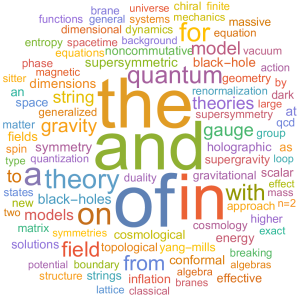
(a) (b)

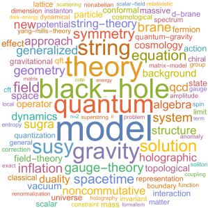
Figure 3: The word clouds for (a) all raw titles (b) all cleaned titles within hep-th. There is a total of 120,249 papers as of the end of 2017. In the raw titles, there are 37,550 unique words and in the cleaned titles, 34,425.

The standard method to present common words in natural language processing is called a word cloud, where words are presented in aggregate, sized according to the frequency of their appearance. We present the word clouds for the raw and cleaned titles in Figure 3.

In the above we encounter a first non-trivial observation. In the raw data, the word “theory” outnumbers the word “model” at nearly two-to-one. After the cleaning process, however, the order is reversed, and the word “model” emerges as the most common word. The explanation involves the grouping of individual words into bi-grams and tri-grams. In particular, the word “theory” ends up in common $n$-grams at a rate that is far larger than the word “model”, which will turn out to be a major discriminatory observation that separates hep-th from other sections of the arXiv.

Clearly, there is more discipline-specific contextual information in the cleaned data. For example, the most common technical word in all hep-th titles is “black-hole”. The most common bi-gram involving the word “theory” is “gauge-theory”, while “string-theory” appears with much lower frequency and is not one of the top-15 words, after cleaning. Note that not every instance of the word “string” appears in a common $n$-gram. Indeed, the word is more often used as an adjective in hep-th titles, as in “string derived models” or “string inspired scenarios”.

For the abstracts of hep-th, we have only the raw data. Given the larger data set, and the prevalence of common, trivial, words, we here give the top 50 words in hep-th abstracts, together with their frequencies:

{the,1174435}, {of,639511}, {in,340841}, {a,340279}, {and,293982}, {we,255299}, {to,252490}, {is,209541}, {for,151641}, {that,144766}, {with,126022}, {are,104298}, {this,98678}, {on,97956}, {by,96032}, {theory,86041}, {as,78890}, {which,71242}, {an,68961}, {be,66262}, {field,65968}, {model,50401}, {from,49531}, {at,46747}, {it,46320}, {can,46107}, {quantum,44887}, {gauge,44855}, {these,39477}, {also,36944}, {show,35811}, {theories,32035}, {string,31314}, {two,30651}, {space,29222}, {models,28639}, {solutions,28022}, {energy,27895}, {one,27782}, {study,26889}, {gravity,25945}, {fields,25941}, {our,24760}, {scalar,24184}, {find,23957}, {between,23895}, {not,23273}, {case,22913}, {symmetry,22888}, {results,22760}

The first technical words which appear are “theory”, “field”, “model”, “quantum” and “gauge”. As mentioned earlier, we have chosen not to “clean” the abstract data. It is interesting to note, however, that if the singular and plural form of words were combined, we would find “theory” and “theories” appearing 118,076 times, or almost once per abstract, with “field”/“fields” appearing in 91,909 abstracts, or just over 76% of the total.

	Raw Data		Cleaned Data
Rank	Bi-gram	Count	Bi-gram	Count
1	of the	9287	separation variable	53
2	in the	6418	tree amplitude	53
3	on the	5342	dark sector	53
4	and the	5118	quantum chromodynamics	53
5	field theory	3592	constrained system	53
6	in a	2452	clifford algebra	53
7	of a	2111	cosmological constraint	53
8	for the	2051	black-hole information	53
9	gauge theories	1789	black ring	53
10	string theory	1779	accelerating universe	53
11	field theories	1468	electroweak symmetry-breaking	53
12	to the	1431	qcd string	53
13	quantum gravity	1412	gravitational instanton	52
14	gauge theory	1350	discrete torsion	52
15	quantum field	1242	electric-magnetic duality	52

Table 3: The fifteen most common bi-grams in hep-th titles, in raw and clean data.

In addition to word frequency in the titles and abstracts, one could also study the $n$-grams. As it is clearly meaningless here to have $n$-grams cross different titles, we will therefore construct $n$-grams within each title, and then count and list all $n$-grams together. The fifteen most common bi-grams in hep-th titles are given in Table 3, again for raw and cleaned data.

There is little scientific content to be gleaned from the raw bi-grams, though we will find this data to be useful in Section 5. In the cleaned bi-grams, many authors reference “separation of variables”, “tree amplitudes”, “dark sectors”, “quantum chromodynamics”, “constrained systems”, “Clifford algebras”, “cosmological constraints”, “black hole information”, “black rings”, “the accelerating universe”, etc. in their titles. It is clear to readers in the hep-th community that in the cleaned data set, many of the bi-grams would themselves be collective nouns if we imposed more rounds of automatic concatenation in the cleaning process.

For completeness, we conclude by giving the 50 most common bi-grams in the raw data for hep-th abstracts:

{{of,the},224990}, {{in,the},115804}, {{to,the},64481}, {{for,the},49847}, {{on,the},46444}, {{that,the},44565}, {{of,a},39334}, {{and,the},38891}, {{can,be},29672}, {{with,the},29085}, {{show,that},27964}, {{we,show},24774}, {{in,a},24298}, {{in,this},23740}, {{it,is},22326}, {{from,the},20924}, {{by,the},20634}, {{to,a},18852}, {{as,a},18620}, {{we,find},17352}, {{we,study},17113}, {{with,a},16588}, {{field,theory},16270}, {{we,also},16184}, {{to,be},15512}, {{is,a},14125}, {{at,the},13722}, {{terms,of},13216}, {{for,a},13112}, {{in,terms},12573}, {{as,the},12233}, {{study,the},11638}, {{we,consider},11481}, {{by,a},11384}, {{of,this},11372}, {{find,that},11288}, {{on,a},11272}, {{is,the},11070}, {{in,particular},10479}, {{which,is},10478}, {{based,on},10123}, {{we,discuss},10051}, {{is,shown},9965}, {{this,paper},9871}, {{of,these},9529}, {{between,the},9480}, {{number,of},9169}, {{string,theory},8930}, {{the,case},8889}, {{scalar,field},8831}

Again, the most common bi-grams are trivial grammatical conjunctions. The first non-trivial combination is “field theory” and then, a while later, “string theory” and “scalar field”. Indeed one would expect these to be the top concepts in abstracts in hep-th. We remark that the current computer moderation of arXiv uses full text, as it is richer and more accurate than titles and abstracts. and establishes a classifier which is continuously updated and uses adaptive length $n$-grams (typically up to n=4) .

4 Machine Learning hep-th

Number of Unique Words Appearing at Least $N$ Times
$N=1$	$N=2$	$N=3$	$N=4$	$N=5$	$N=6$	$N=7$	$N=8$	$N=9$	$N=10$
34425	16105	11642	9516	8275	7365	6696	6179	5747	5380

Table 4: Number of unique words appearing at least $N$ times in hep-th titles. The 16,105 words with at least two appearances were utilized as a training set for Word2vecfor the purposes of the current section.

Having suitably prepared a clean dataset, we then trained Word2vec on the collection of titles in hep-th. Given the typically small size of titles in academic papers, we chose a context window of length $5$. To minimize the tendency of the neural network to focus on outliers, such as words that very rarely appear, we dropped all words that appear less than twice in the data set for the purpose of training. As Table 4 indicates, that meant that a little over half of the unique words in the hep-th titles were not employed in the training. Finally, we follow standard practice in the literature by setting $N=400$ neurons for the hidden layer, using the CBOW model. The result is that each of the non-trivial words is assigned a vector in $\mathbb{R}^{400}$ so that the partition function (7) is maximized.

4.1 Word Similarity

Once the word embedding has been established, we can form cosine distances in light of our definition of similarity and dissimilarity in Definition 5. This is our first glimpse into the ability of the neural network to truly capture the essence of syntax within the high energy theory community: to view which pairs of words the neural network has deemed “similar” across the entire corpus of hep-th titles.

Overall, we find that the neural network in Word2vec does an admirable job in a very challenging area of context. Consider the bi-gram “super Yang-Mills”, often followed by the word “theory”. In step #5 of the initial processing of the data, described in Section 3.2, we would have manually replaced this tri-gram with the acronym “sym”, since “SYM” would be immediately recognized by most practitioners in our field as “super Yang-Mills”. Thus the tri-gram “supersymmetric Yang-Mills theory”, a quantum field theory described by a non-Abelian gauge group, will be denoted as ‘sym’. Some representative word similarity measurements are

$$d(\text{`sym'},\text{`sym'}) = 1.0,$$

$$d(\text{`sym'},\text{`n=4'}) = 0.9763,$$

$$d(\text{`sym'},\text{`matrix-model'}) = 0.9569,$$

$$d(\text{`sym'},\text{`duality'}) = 0.9486,$$

$$d(\text{`sym'},\text{`black-hole'}) = 0.1567,$$

$$d(\text{`sym'},\text{`dark-energy'}) = -0.0188,$$

$$d(\text{`sym'},\text{`dark-matter'}) = -0.0370\,.$$ (10)

The above means that, for example, “sym” is identical to itself (a useful consistency check), close to “duality”, and not so close to “dark-matter”, within our context windows. To practitioners in our field, these relative similarities would seem highly plausible.

Word	Most Similar	$d(w_{1},w_{2})$	Least Similar	$d(w_{1},w_{2})$
model	theory	0.7775	entropy	-0.0110
theory	action	0.7864	holographic	0.0079
black-hole	rotating	0.9277	lattice	0.1332
quantum	entanglement	0.8645	sugra	0.1880
gravity	massive-gravity	0.8315	$g^{4}$	0.0618
string	string-theory	0.9016	approach	0.0277
susy	gauged	0.9402	energy	0.0262
solution	massive-gravity	0.6900	holographic	0.0836
field	massless	0.8715	instanton	0.0903
equation	bethe-ansatz	0.8271	matter	0.0580
symmetry	transformations	0.9286	gravitational	0.0095
spacetime	metric	0.8560	amplitude	0.2502
brane	warped	0.9504	method	0.1706
inflation	primordial	0.9200	cft	0.1137
gauge-theory	sym	0.8993	universe	0.1507
system	oscillator	0.8729	compactification	0.1026
geometry	manifold	0.8862	qcd	0.1513
sugra	gauged-sugra	0.8941	relativistic	0.1939
new	type	0.8807	state	-0.1240
generalized	class	0.9495	effect	0.0658

Table 5: The twenty most frequent words in hep-th titles. Included is the word with the largest and smallest values of the word-distance $d(w_{1},w_{2})$ (from equation 8), as computed by Word2vec.

We computed the similarity distance (8) for all possible pairs of the 9516 words in hep-th titles which appear at least four times in the set. The twenty most frequent words are given in Table 5, along with the word for which $d(w_{1},w_{2})$ is maximized, and where it is minimized. We refer to these words as the ‘most’ and ‘least’ similar words in the set.

Some care should be taken in interpreting these results. First, authors clearly use a different type of syntax when constructing a paper title than they would when writing an abstract, the latter being most likely to approximate normal human speaking styles. The semi-formalized rules that govern typical practice in crafting titles will actually be of interest to us in Section 5, when we compare these rules across different sections of arXiv.

The second caveat is that for two words to be considered similar, it will be necessary that the two words (1) appear sufficiently often to make our list, and (2) appear together in titles, within five words of one another, with high regularity. Thus we expect words like “black hole” and “rotating”, or “spacetime” and “metric”, to be naturally similar in this sense. How then should we interpret the antipodal word, which we designate as the “least similar”? And what of the vast number of words whose cosine distance vanishes with respect to a particular word?

Recall the discussion in Section 2.3. The neural network establishes the vector representation of each word by attempting to optimize contextual relations. Thus two words will appear in the same region of the vector space if they tend to share many common words within their respective content windows. Inverting this notion, two words will be more likely to appear in antipodal regions of the vector space if the words they commonly appear with in titles are fully disjoint from one another. Thus “sym” (supersymmetric Yang-Mills theory) is not necessarily the ‘opposite’ of “dark matter” or “dark energy” in any real sense, but rather the word “sym” tends to appear in titles surrounded by words like “duality” or “matrix model”, which themselves rarely appear in titles involving the words “dark matter” or “dark energy”. Thus the neural network located these vectors in antipodal regions of the vector space.

The results of Table 5 also indicate that strictly negative values of $d(w_{1},w_{2})$ are, in fact, quite rare. So, for example, the word that is “least similar” to “spacetime” is “amplitude”, with $d(\text{`spacetime'},\text{`amplitude'})=0.25$. Part of the reason for this behavior is that Table 5 is presenting the twenty most frequent words in hep-th titles. Thus a word like “spacetime” appears in may titles, and develops a contextual affinity with a great many of the 9516 words in our dataset. As a consequence, no word in the hep-th title corpus is truly ‘far’ from the word “spacetime”.

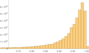
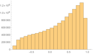
Figure 4: Distribution of similarity distances, defined by (8), for all pairs of words with at least four appearances in the corpus. The left panel gives the distribution for titles in hep-th. The right panel is the distribution for a similarly-sized collection of news headlines from Times of India. While both distributions show a clustering effect of words around certain dominant words, the shape of the distribution for hep-th shows a much tighter ‘conical’ cluster than the hews headlines. In particular, we note the vertical scale in the two panels, in which negative similarity distances are essentially absent in hep-th titles, but reasonably frequent in the Times of India headlines.

The relative lack of negative similarity distances, and the lop-sided nature of the vector space embedding produced by Word2vec, are striking for the hep-th titles. However, such behavior was noted in recent work by Mimno and Thompson on natural language processing with the skip-gram method [24]. The authors observed that data sets tended to cluster in a cone around certain dominant words that appear frequently in context windows, such as the words like “model” and “theory” in our case. This is certainly the case with our data. A histogram of the $d(w_{1},w_{2})$ values for the 9516 words in hep-th titles which appear at least four times is given in the left panel of Figure 4. The overwhelming majority of word pairs have similarity distances satisfying $d(w_{1},w_{2})\geq 0.9$, with a mean value given by

$$d(w_{1},w_{2})\big{|}_{\rm hepth}=0.9257\pm 0.0889\,.$$ (11)

It might be thought that this extreme clustering is an artefact of the small size of the data set, or the restriction to words that appear at least four times. But relaxing the cut-off to include all pairs of words that appear two or more times changes neither the average similarity distance nor the shape of the histogram. As a control sample, we also trained Word2vec to produce a word embedding for the 22,950 unique words contained in 20,000 titles for news articles appearing in the Times of India [32]. The same clustering affect occurs in this data sample, as can be seen by the histogram in the right panel of Figure 4, but to a much more moderate extent. In fact, this data set contains a significant number of negative $d(w_{1},w_{2})$ values, with a mean value given by

$$d(w_{1},w_{2})\big{|}_{\rm headlines}=0.2642\pm 0.5171\,.$$ (12)

We will return to this Times of India dataset in Section 6.

4.2 Linear Syntactic Identities

With a measure of similarity, we can now seek examples of meaningful syntactic identities, analogous to (2). This is done by finding the nearest vector to the vector sum/difference amongst word-vectors. For example, we find that

$$\text{`holography'}+\text{`quantum'}+\text{`string'}+\text{`ads'}=\text{`extremal-black-hole'}\ .$$ (13)

This is a correct expression, in that a hypothetical title containing the four words on the left hand side could plausibly contain the one on the right hand side. This is very interesting because by context alone, we are uncovering the syntax of hep-th, where likely concepts appear together. This is exactly the purpose of Word2vec, to attempt to study natural language through the proximity of context.

Another good example is

$$\text{`bosonic'}+\text{`string-theory'}=\text{`open-string'}\ .$$ (14)

Of course, we need to take heed. It is not that the neural network has learned physics well enough to realize that the bosonic string has an open string sector; it is just that the neural network has learned to associate “open-string” as a likely contextual neighbor of “bosonic” and “string theory”. One could also add word-vectors to themselves (subtracting would simply give the word closest to the $0$-vector), such as (dropping the quotation marks for convenience):

gravity  +  gravity = massive-gravity
string  +  string = string-theory
quantum  +  quantum = quantum-mechanics
holography  +  holography = microscopic

We will note that there is not much content to these identities. It is not at all clear what scaling means in this vector space.

We can systematically construct countless more “linear syntactic identities” from, say, our most common words. For instance those of the form ‘a’ + ‘b’ = ‘c’ include:

symmetry  +  black-hole  =  killing
spacetime  +  inflation  =  cosmological-constant
string-theory  +  spacetime  =  near-horizon
black-hole  +  holographic  =  thermodynamics
string-theory  +  noncommutative  =  open-string
duality  +  gravity  =  ‘d=5’
black-hole  +  qcd  =  plasma
symmetry  +  algebra  =  group

The physical meaning of all of these statements are clear to a hep-th reader.

One can as well generate higher order examples of the form ‘a’ + ‘b’ = ‘c‘ + ‘d’, such as

field  +  symmetry  =  particle + duality
system  +  equation  =  classical + model
generalized  +  approach  =  canonical + model
equation  +  field  =  general + system
space  +  black-hole  =  geometry + gravity
duality  +  holographic  =  finite + string
string-theory + calabi-yau = m-theory + g2

as well as even longer ones:

string-theory + calabi-yau + f-theory = orientifold
quiver + gauge-theory + calabi-yau = scft
brane + near-horizon - worldvolume = warped

It is amusing that we can find many such suggestive identities. On the other hand, we also find many statements which are simply nonsensical.

5 Comparisons with Other arXiv Sections

In the previous section, we performed some basic descriptive analyses of the vocabulary of the hep-th community, demonstrated the power of Word2vec in performing textual analysis, illuminated the nature of the vector space created by the neural network output, and used this space to study word correlations and linear syntactic identities within the space generated by the corpus of all hep-th titles. We find these items interesting (or at least amusing) in their own right, and expect that there is much more that can be extracted by expert linguists or computer scientists.

As an application, in this section we would like to use the tools introduced above to perform an affinity analysis between the socio-linguistics of the hep-th community and sister communities that span theoretical high energy physics. There are many sections on arXiv to which a great number of papers on hep-th are cross-listed. Similarly, authors who post primarily to hep-th often also post to other sections, and vice versa. This was particularly relevant prior to mid-2007, when each individual manuscript was referred to by its repository and unique number, and not solely by a unique number alone. As described in Section 3.1, the most pertinent physics sections besides hep-th are

• hep-ph (high energy phenomenology);

• hep-lat (high energy lattice theory);

• math-ph (mathematical physics);

• gr-qc (general relativity and quantum cosmology).

It is therefore potentially interesting to perform a cross-sectional comparative study.

What sorts of phenomena might we hope to identify by such a study? Loosely speaking, we might ask where authors in hep-th lie in the spectrum between pure mathematics and pure observation. Can we quantify such a notion by looking at the language used by authors in these various sections? The answer will turn out to be, in large part, affirmative. Intriguingly, we will see that the distinctions between the sub-fields is not merely one of subject matter, as there is a great deal of overlap here, but often it is encoded in the manner in which these subjects are described.

5.1 Word Frequencies

arXiv	No. of	Median	Mean	Number of	Unique Word
Section	Papers	Length	Length	Unique Words	Fraction
hep-th	120,249	5	5.08	34,425	4.66%
hep-ph	133,346	5	5.58	39,611	4.59%
hep-lat	21,123	5	5.58	9,431	6.96%
gr-qc	69,386	5	5.34	22,357	5.32%
math-ph	51,747	6	6.01	25,516	7.62%

Table 6: Gross properties of the collection of titles of the five arXiv sections studied in this paper, now after the cleaning process (described in Section 3.2) has been performed. The final column gives the number of unique words divided by the total number of words, after cleaning.

As in the previous sections, we first clean the data to retain only relevant physics-concept related words. We again focus on the titles of papers in the five repositories. Some statistics for the data sets, in raw form, were given in Table 1. After the cleaning process titles are typically shortened, and the number of unique words diminishes somewhat, as is shown in Table 6. Again, the five repositories are roughly equal in their gross properties. We present the word-clouds for the four new repositories, after the cleaning procedure, in Table 16, found in Appendix B.

At this point one could pursue an analysis for each repository along the lines of that in Section 4. However, we will be less detailed in our study of the other four sections of arXiv, as our focus in this section is two-fold: (1) to begin to understand similarities and differences between the authors in these five groupings, as revealed by their use of language, and (2) lay the groundwork for the classification problem that is the focus of Section 6.

hep-th		hep-ph		hep-lat		gr-qc		math-ph
Word	%	Word	%	Word	%	Word	%	Word	%
model	0.80	model	0.84	lattice	1.91	black-hole	1.17	model	1.06
theory	0.62	qcd	0.58	qcd	1.43	gravity	0.96	equation	0.93
black-hole	0.60	decay	0.53	lattice-qcd	1.39	spacetime	0.75	quantum	0.92
quantum	0.57	effect	0.53	model	0.95	model	0.70	system	0.75
gravity	0.51	lhc	0.51	quark	0.58	quantum	0.58	solution	0.59
string	0.48	dark-matter	0.46	theory	0.54	cosmology	0.58	theory	0.49
susy	0.45	neutrino	0.41	mass	0.53	universe	0.55	operator	0.48
solution	0.37	mass	0.38	fermion	0.53	theory	0.52	algebra	0.45
field	0.32	production	0.38	chiral	0.51	gravitational-wave	0.50	potential	0.44
equation	0.32	susy	0.37	meson	0.41	inflation	0.46	symmetry	0.42

Table 7: Top ten most frequent words in the titles of the five arXiv sections, after cleaning. The percentage is the number of appearances of the particular word divided by the total of all words (including multiplicities).

We therefore begin with a focus on the most common ‘key’ words in each section of arXiv. In Table 7 we list the ten most common words in the titles of papers in each repository. We also give the overall word frequency for each word, normalized by the total number of words. Thus, for example, 1.91% of all the words used in hep-lat titles is the specific word “lattice”, which is perhaps unsurprising. Indeed, the word frequencies in Table 7 are as one might expect if one is familiar with the field of theoretical high energy physics.

Many words appear often in several sections of arXiv, others are common in only one section. Can this be the beginning of a classification procedure? To some extent, it can. For example, the word “model” is a very common word in all five sections, while “theory” fails to appear in the top ten words only for hep-ph. However, this is deceptive, since it would be ranked number 11 if we were to extend the table. Despite such obvious cautions, there is still some comparative information which can be extracted from Table 7.

Top Word	hep-th	hep-ph	hep-lat	gr-qc	math-ph
black-hole	3	-	-	1	-
equation	10	-	-	-	2
gravity	5	-	-	2	-
mass	-	8	7	-	-
model	1	1	4	4	1
quantum	4	-	-	5	3
solution	8	-	-	-	5
susy	7	10	-	-	-
theory	2	-	6	8	6

Table 8: Words which are among the top ten most frequent for more than one arXiv section, with the rank of the word in those sections. The dashes ‘-’ mean that the particular words has not made it into the top 10 of the specified arXiv section.

Consider Table 8, in which we present only those words in Table 7 which appear in two or more sections of the arXiv. We again see the universal importance of words like “model” and “theory”, but we also begin to see the centrality of hep-th emerge. Indeed, it was for this reason that we chose to focus on this section of the arXiv in the first place. Note that the words which are frequently found in hep-th tend to be frequent in other sections. Perhaps this represents some aspect of generality in the subject matter of hep-th, or perhaps it is related to the fact that amongst the other four sections, hep-th is far more likely to be the place where a paper is cross-listed than any of the remaining three sections.

What is more, even at this very coarse level, we already begin to see a separation between the more mathematical sections (hep-th, gr-qc, and math-ph), and the more phenomenological sections (hep-ph and hep-lat). Such a divide is a very palpable fact of the sociology of our field, and it is something we will see illustrated in the data analysis throughout this section.

From the point of view of document classification, the simple frequency with which a word appears is a poor marker for the section of arXiv in which it resides. In other words, if a paper contains the word “gravity” in its title, it may very likely be a gr-qc paper, but the certainty with which a classifying agent – be it a machine or a theoretical physicist – would make this assertion would be low. As mentioned in Section 2.5, term frequency-inverse document frequency (tf-idf) is a more nuanced quantity which captures the relative importance of a word of $n$-gram.

Recall that there are three important concepts when computing tf-idf values. First there are the words themselves, then there are the individual documents which, collectively, form the corpus. If our goal is to uncover distinctions between the five arXiv sections using tf-idf values, it might make sense to take each paper as a document, with the total of all documents in a given section being the corpus. If we were studying the abstracts, or even the full text of the papers themselves, this would be the best approach. But as we are studying only the titles here, a problem immediately presents itself.

After the cleaning process, in which small words are removed and common bi-grams are conjoined, a typical title is quite a small “document”. As Table 6 indicates, the typical length of the document is five or six words. Thus, it is very unlikely that the term frequency across all titles will deviate greatly from the document frequency across the titles. This is borne out in the data. Taking the union of all words which rank in the top 100 in frequency across the five sections, we obtain 263 unique words. Of these 42.3% never appear more than once in any title, in any of the five sections. For 63.5% of the cases, the term frequency and document frequency deviate by no more than two instances, across all five arXiv sections. Thus, tf-idf computed on a title-by-title basis is unlikely to provide much differentiation, as common words will have very similar tf-idf values.

Word	hep-th	hep-ph	hep-lat	gr-qc	math-ph
chiral-perturbation-theory	0.71	1.45	1.24	0.	0.15
cmb	1.36	1.43	0.	1.4	0.49
cosmological-model	4.73	0.	0.	5.86	0.
finite-volume	0.95	1.08	1.2	0.	0.46
ising-model	2.82	0.	2.74	0.	2.78
landau-gauge	2.35	2.5	2.72	0.	0.
lattice-gauge-theory	2.66	2.39	2.97	0.	0.
lhc	1.19	1.87	0.69	0.9	0.
modified-gravity	2.89	2.42	0.	3.22	0.
mssm	1.05	1.58	0.31	0.55	0.
neutrino-mass	2.24	3.54	0.	0.35	0.
new-physics	0.92	1.57	0.31	0.15	0.
nucleon	0.78	1.65	1.35	0.15	0.
quantum-mechanics	1.49	1.15	0.	1.28	1.37
quark-mass	2.07	3.07	2.72	0.	0.
scalar-field	1.51	1.34	0.	1.56	1.12
schrodinger-operator	0.	0.	0.	0.	10.08
string-theory	1.67	1.28	0.	1.28	0.97
wilson-fermion	0.	0.	8.87	0.	0.

Table 9: Term frequency-inverse document frequency (tf-idf) for certain key words. The corpus here is the set of all titles for all papers in all five sections of the arXiv. These sections become the five documents of the corpus.

Therefore, we will instead consider an alternative approach. We let the corpus be all titles for all five sections of the arXiv; in other words, we treat the entire (theoretical high energy) arXiv as a single corpus. The collections of five titles form the five “documents” in this corpus. While this clearly implies some blurring of context, it gives a sufficiently large data set, document-by-document, to make tf-idf meaningful.

We provide the tf-idf values for a representative set of words in the five arXiv sections in Table 9. Recall that words that are extremely common in individual contexts (here, specifically, paper titles), across an entire arXiv section, will have very low values of tf-idf. For example, words such as “theory” and “model” appears in all sections, and would therefore receive a vanishing value of tf-idf. Therefore, it is only illustrative to include words which do not trivially have a score of zero for all sections. Our collection of titles is sufficiently large in all cases that there are no words which appear in all paper titles, even prior to the cleaning step, which removes small words like “a” and “the”. Therefore, entries which are precisely zero in Table 9 are cases in which the word appears in none of the paper titles for that section of arXiv.

So, for example, we see that, interestingly, the word “schrodinger-operator” appears only in math-ph but not in any of the others. This is, in fact, the word with the highest tf-idf score by far. Of course, the Schrd̈inger equation is ubiquitous in all fields of physics, but only in math-ph – and not even in hep-th – is its operator nature being studied intensively. Likewise, the Wilson fermion is particular to hep-lat. The word “string-theory” is mentioned in all titles except, understandably, in hep-lat.

Using machine learning techniques to classify arXiv titles will be the focus of our next section, but we can take a moment to see how such an approach could potentially improve over a human classifier – even one with expertise in the field. A full-blown tf-idf analysis would not be necessary for a theoretical physicist to surmise that a paper whose title included the bi-gram “Wilson fermion” is very likely from hep-lat. But, surprisingly, having “lattice gauge theory” in the title is not a very good indicator of belonging to hep-lat. Nor is it sufficient to assign gr-qc to all papers with “modified gravity” in its title.

5.2 Common Bi-grams

As before, from mono-grams (individual words) we proceed to common $n$-grams. In this section we will concentrate on bi-grams for simplicity. Common 3-grams and 4-grams for the various sections can be found in Appendix B. It is enlightening to do this analysis for both the cleaned data (for which we will extract subject content information), as well as for the raw data, which retains the conjunctions and other grammatically interesting words. The latter should give us an idea of the syntax of the language of high energy and mathematical physics across the disciplines.

hep-th	hep-ph	hep-lat	gr-qc	math-ph
of the	of the	of the	of the	of the
in the	in the	lattice qcd	in the	on the
on the	dark matter	in the	on the	for the
and the	and the	on the	and the	in the
field theory	at the	the lattice	of a	and the
in a	on the	gauge theory	quantum gravity	of a
of a	in a	and the	dark energy	in a
for the	the lhc	in lattice	in a	to the
gauge theories	to the	from lattice	gravitational waves	for a
string theory	for the	lattice gauge	general relativity	on a
field theories	standard model	qcd with	for the	solutions of
to the	corrections to	at finite	scalar field	field theory
quantum gravity	production in	gauge theories	black-holes in	of quantum
gauge theory	production at	study of	gravitational wave	approach to
quantum field	from the	for the	with a	quantum mechanics

Table 10: The top 15 most commonly encountered bi-grams in the raw data, for each of the five sections of arXiv. Bi-grams are listed from most frequent (top) to least frequent (bottom).

Raw Data:

The top 15 most commonly encountered bi-grams in the raw data, for each of the five sections of arXiv, are presented in Table 10, in descending order of frequency. At first glance, the table may seem to contain very little distinguishing information. Clearly certain linguistic constructions, such as “on the” and “on a”, are commonly found in the titles of academic works across many disciplines. One might be tempted to immediately remove such “trivial” bi-grams and proceed to more substantive bi-grams. But, in fact, there is more subtlety here than is immediately apparent. Let us consider the twelve unique, trivial bi-grams in the table above. They are given in Table 11 for each repository, with their ranking in the list of all bi-grams for that repository.

	arXiv Repository Rank
Bi-gram	hep-th	hep-ph	hep-lat	gr-qc	math-ph
of the	1	1	1	1	1
in the	2	2	3	2	4
on the	3	6	4	3	2
and the	4	4	7	4	5
in a	6	7	19	8	7
of a	7	16	35	5	6
for the	8	10	15	11	3
to the	12	9	21	16	8
on a	17	152	28	38	10
from the	19	15	27	27	74
with a	21	27	57	15	16
at the	87	5	97	114	224

Table 11: Contextually ‘trivial’ bi-grams across five arXiv sections. The entry gives the rank of the bi-gram, in terms of the bi-gram frequency, after only removing capitalization.

Three things immediately stand out. The first is the universal supremacy of the bi-gram “of the”. The second is the presence of “at the” in hep-ph at a high frequency, yet largely absent from the other repositories. But this is clearly understood as the likelihood of hep-ph titles to include phrases like “at the Fermilab Tevatron”, or “at the LHC”, in their titles. This is unique to hep-ph among the five categories studied here. Finally, there is the construction “on a”, which appears significantly only in hep-th and math-ph, and is very rare in hep-ph titles.

Again, this is easily understood, as the phrase “on a” generally precedes a noun upon which objects may reside. That is, plainly speaking, a surface. And the study of physics on surfaces of various sorts is among the most mathematical of the physical pursuits. So this meta-analysis of physics language syntax would seem to indicate a close affinity between hep-th and math-ph, and a clear distinction between hep-ph and all the other theoretical categories. While this may confirm prejudices within our own fields, a closer inspection of these trivial bi-grams is warranted.

	hep-th	hep-ph	hep-lat	gr-qc	math-ph
hep-th	1	0.29	0.94	0.99	0.96
hep-ph	0.29	1	0.39	0.38	0.12
hep-lat	0.94	0.39	1	0.90	0.84
gr-qc	0.99	0.38	0.90	1	0.95
math-ph	0.96	0.12	0.84	0.95	1

Table 12: Treating the columns of Table 11 as vectors in $\mathbb{R}^{12}$, the cosine of the angles between the various vectors is given.

Considering Table 11 more seriously, we can treat the columns as vectors in a certain space of trivial bi-grams (not to be confused with word-vectors which we have been discussing). A measure of affinity between the authors of the various arXiv sections would then be the cosine of the angle between these vectors. The value of these cosines is presented in Table 12.

What emerges from Table 12 is quite informative. It seems that the simplest of our community’s verbal constructs reveal a great deal about how our colleagues organize into groups. Our central focus is the community of hep-th, and it is somewhat reassuring to see that the trivial bi-gram analysis reveals that this section has relatively strong affinity with all of the arXiv sections studied. Yet there is clearly a break between hep-th and hep-ph  a distinction we will comment upon later. Clearly, some of this is driven by the “at the” bi-gram, suggesting (quite rightly) that hep-ph is the most experimentally-minded of the arXiv sections studied here. But even if this particular bi-gram is excluded from the analysis, hep-ph would still have the smallest cosine measure with hep-th.

Clearly, the trivial bi-gram analysis suggests that our group of five sections fragments into one section (hep-ph), and the other four, which cluster rather tightly together. Among these remaining four, hep-lat is slightly the outlier, being more closely aligned with hep-th than the other sections. Most of these relations would probably not come as a surprise to authors in the field, but the fact that the computer can make distinctions in such a specialized sub-field, in which even current practitioners would have a difficult time making such subtle differentiation, is intriguing.

Cleaned Data:

After the cleaning process, which includes the two rounds of computer generated word concatenations, described in Appendix A, the majority of the most common bi-grams in each section of the arXiv will have been formed into single words. What remains reveals something of the specific content areas unique to each branch of theoretical particle physics. The 15 most frequent bi-grams after cleaning are given in Table 13.

hep-th	{separation,variable}, {tree,amplitude}, {dark,sector}, {quantum,chromodynamics},
	{constrained,system}, {clifford,algebra}, {cosmological,constraint}, {black-hole,information},
	{black,ring}, {accelerating,universe}, {electroweak,symmetry-breaking}, {qcd,string},
	{gravitational,instanton}, {discrete,torsion}, {electric-magnetic,duality}
hep-ph	{first-order,phase-transition}, {chiral-magnetic,effect}, {double-parton,scattering},
	{littlest-higgs-model,t-parity}, {momentum,transfer}, {extensions,sm}, {magnetic,catalysis},
	{jet,substructure}, {matter,effect}, {energy,spectrum}, {spin-structure,function},
	{equivalence,principle}, {light-scalar,meson}, {au+au,collision}, {searches,lhc}
hep-lat	{flux,tube}, {perturbative,renormalization}, {imaginary,chemical-potential}, {ground,state},
	{gluon,ghost}, {electroweak,phase-transition}, {string,breaking}, {physical,point},
	{2+1-flavor,lattice-qcd}, {lattice,action}, {2+1-flavor,qcd}, {random-matrix,theory},
	{effective,action}, {screening,mass}, {chiral,transition}
gr-qc	{fine-structure,constant}, {extreme-mass-ratio,inspirals}, {closed-timelike,curves}, {bulk,viscosity},
	{born-infeld,gravity}, {dirac,particle}, {ds,universe}, {einstein-field,equation}, {fundamental,constant},
	{topologically-massive,gravity}, {bose-einstein,condensate}, {higher-dimensional,black-hole},
	{hamiltonian,formulation}, {static,black-hole}, {generalized-second,law}
math-ph	{time,dependent}, {external,field}, {thermodynamic,limit}, {long,range}, {variational,principle},
	{loop,model}, {minkowski,space}, {fokker-planck,equation}, {characteristic,polynomials},
	{hamiltonian,dynamics}, {integral,equation}, {configuration,space}, {lattice,model},
	{constant,curvature}, {gaussian,free-field}

Table 13: Most common bi-grams in cleaned data, after two rounds of automated concatenation.

While these bi-grams certainly capture important areas of theoretical physics research in each section of the arXiv  they are somewhat deceiving. For example, the “chiral magnetic effect” – a phenomenon of induced chiral behavior in a quark-gluon plasma – has been the subject of study of roughly five papers per year in hep-ph over the last decade. But it would be wrong to suppose that it is more commonly studied than “searches (at the) lhc”, or “extensions (to the) sm”, where the acronyms stand for Large Hadron Collider and Standard Model, respectively.

In this case, we see a potential drawback of the automated concatenation described in Appendix A: whereas tightly related topics will naturally be grouped together, some of the diversity of subject matter in each section of the arXiv will be obscured. So, for example, in step #5 in Section 3.2 we turn common compound expressions like “operator product expansion” into the acronym “ope”. In addition, a handful of very common bi-grams were hyphenated, such as “dark matter” becoming “dark-matter”. Cosmological dark matter is a topic of investigation in hep-ph which appears to be totally missing in Table 13! However, what has happened is that various sub-categories of postulated dark matter candidates have been concatenated in the automated steps which follow, producing “cold-dark-matter”, “warm-dark-matter”, “fuzzy-dark-matter”, etc. The total frequency of appearance for “dark matter” itself is thus distributed across many ‘words’ in the total corpus.

To take another example, particle physicists of a certain age will remember the flurry of papers appearing (primarily) in hep-ph in the early 2000’s with the bi-gram “little Higgs” in the title. Indeed, for a certain period of time it seemed that every paper in hep-ph concerned this alternative to the traditional Higgs mechanism of the Standard Model. From this were spun many off-shoots with their ever-more creative names: “littler Higgs”, “littlest Higgs” (a hint of which appears in Table 13), “fat Higgs”, “thin Higgs”, etc. Where are all the “little Higgs” papers in our study?

Key Word	hep-th	hep-ph	hep-lat	gr-qc	math-ph
theory	290	72	144	141	131
model	259	251	185	178	228
Higgs	21	123	24	11	5
dark	3	8	–	8	1
black	6	1	–	9	3
natural	2	2	–	1	–
conformal	33	5	14	27	25

Table 14: Number of unique bi-grams formed with seven key words, across the five arXiv sections. Frequencies are computed from processed data (small words are removed but automated concatenation is not performed).

The answer, as Table 14 shows, is that they are still there – only hidden. In the table, we work with processed data, which (as described in Section 3.2) is data in which the first five steps of the cleaning process – through the removal of small words – is performed, but prior to the automated concatenation of common bi-grams. What is given in Table 14 is the number of unique bi-grams constructed with seven very common key words, for each of the five sections. To construct the Table above, we only considered the top-6000 bi-grams in each section, ranked by frequency of appearance.

First we remark on the sheer number of bi-grams formed with “theory” and “model”. Prior to automated concatenation, “model” far outstrips “theory” in hep-ph, and to a lesser extent in math-ph. After the automated concatenation (i.e. in the cleaned data), “model” will be one the most common, or nearly most common, words in all five sections, as shown in Table 7. As we remarked in Section 3.3, it is this automated concatenation that will eventually reduce the frequency of the stand-alone word “theory” in hep-th.

The other five words reveal a great deal about the subject matter of the five arXiv sections, as well as demonstrating the creativity of the high energy theory community in creating new bi-grams. This is particularly so, as expected, in hep-ph’s treatment of the word “Higgs”, in which an astounding 123 bi-grams are identified involving this word, including everything from “abelian Higgs” to “Higgs vacuum”. The distinction between the phenomenological (hep-ph and hep-lat) and more formal sections is evident in the number of bi-grams involving “conformal”, with hep-th leading the group. It seems hep-ph concerns itself more with “dark” objects (“atoms”, “forces”, “gauge”, “photon”, “radiation”, “sector”, “side”) than “black” ones; it is vice versa for hep-th (“black” plus “brane”, “hole”, “objects”, “p-brane”, “ring”, “string”); and gr-qc is concerned with both in equal measure. Finally, despite the frequent use of “natural” in our community – and its ubiquitous adjectival noun form, “naturalness” – this word appears paired in a bi-gram with only two words with any great regularity: “inflation” and “susy (supersymmetry)”.

5.3 Comparative Syntactic Identities

We conclude this amusing bit of navel-gazing with a comparison of the five arXiv sections using the vector space word embeddings produced by Word2vec. As in Section 4, we train Word2vec on the five lists of words formed from the titles of the five sections, after the full cleaning procedure is performed. What we are seeking is differences in the way certain common words are represented in the five constructed vector spaces.

It is intriguing to consider how linear syntactic identities, such as those identified in Section 4.2, are modified when we map words from one vector space embedding to another. It would be particularly interesting to see if, in different sections of the arXiv, the same left-hand side of a linear syntactic identity ‘a’ + ‘b’ = ‘c’ leads to completely different ‘c’ in different spaces. This would be indicative of the very nature of the terminologies of the fields.

Many possible ‘a’ + ‘b’ pairs can be constructed, though very frequently one of the members of the (‘a’,‘b’) pair happens to be seldom used in at least one of the five arXiv sections. One word which appears frequently with many partners is the word ‘spin’. Some syntactic identities using this word include:

hep-th:  spin  +  system  =  free
hep-ph:  spin  +  system  =  1/2
hep-lat:  spin  +  system  =  ising
gr-qc:  spin  +  system  =  initial-data
math-ph:  spin  +  system  =  charged

hep-th:  spin  +  dynamics  =  point
hep-ph:  spin  +  dynamics  =  chromofield
hep-lat:  spin  +  dynamics  =  geometry
gr-qc:  spin  +  dynamics  =  orbiting
math-ph:  spin  +  dynamics  =  interacting

hep-th:  spin  +  effect  =  electron
hep-ph:  spin  +  effect  =  role
hep-lat:  spin  +  effect  =  bound-state
gr-qc:  spin  +  effect  =  detector
math-ph:  spin  +  effect  =  glass

What these identities reveal is that ‘spin’ is used in very general contexts in both hep-th and hep-ph, but in rather more specific contexts in the other three sections. So, for example, in gr-qc a topic of inquiry may be the dynamics of spinning objects orbiting a black hole, whereas the thermodynamics and stability properties of spin glasses has been a common topic of research in math-ph.

We conclude this section with the syntactic identity formed from perhaps the two most fundamental concepts in theoretical particle physics: “field theory” (the tool with which all of our calculations are performed), and “scattering” (the primary observable we labor to compute). Across the five disciplines, these two concepts generate the following:

hep-th:  scattering  +  field-theory  =  green-function
hep-ph:  scattering  +  field-theory  =  dispersion-relation
hep-lat:  scattering  +  field-theory  =  wave-function
gr-qc:  scattering  +  field-theory  =  bms
math-ph:  scattering  +  field-theory  =  internal

Note that “bms” here refers to the Bondi-Metzner-Sachs (BMS) group, a symmetry property of asymptotically-flat Lorentzian spacetimes, which was shown by Strominger to be a symmetry of the $S$-matrix in perturbative quantum gravity [33].

6 Title Classification

The previous sections would be of some mild interest to theoretical particle physicists who routinely publish in the areas covered by our five arXiv sections. But for practicing data scientists, what is of interest is the ability of the word embeddings to generate a classification algorithm that accurately and efficiently assigns the proper arXiv section to a given paper title. In our context, the question is naturally

Question: Given a random title (not even necessarily a legitimate physics title), can a neural network decide to which section on the arXiv is it likely to belong?

It turns out that one of the most powerful uses for Word2vec is classification of texts [34]. Indeed, document classification is one of the key tasks a neural network is asked to perform in natural language processing generally.

Classification is the canonical problem in supervised machine learning, and there are many possible approaches. The preceding sections have provided us with insights that will prove of value. In particular, ‘cleaning’ the data allowed us to examine certain contextual relations and make more meaningful frequency statements about certain concepts. Nevertheless, it eliminated some information that may be useful, such as the pattern of small words like conjunctions, and it tended to bury certain key descriptors (like ‘dark’) by embedding them in multiple hyphenated words. We will therefore train our classifier with raw data, with the only processing being the removal of upper-case letters.

The algorithm we will choose is the mean word-vector method [34], and it proceeds as follows:

• Combine all titles from all the relevant sections from arXiv; establish a word-vector for each word using Word2vec’s CBOW neural network model. This gives a single vector space $V$ consisting of many 400-vectors (recall that our convention is such that each word-vector is an element of $\mathbb{R}^{400}$);

• Subsequently, for each title, considered as a list of words, take the component-wise mean of the list of word-vectors; thus each title is associated with a single vector in $V$;

• Establish labelled data $D$ consisting of entries (Title₁, $i$), (Title₂, $i$), …, (Title_k, $j$), (Title_k+1, $j$), …over all arXiv sections under consideration; Here $i,j,\ldots\in\{1,2,3,4,5\}$ specifies the 5 sections, respectively, hep-th, hep-ph, hep-lat, gr-qc and math-ph;

• Construct a “training set”, say 7000 random samples from $D$ and use one’s favourite classifier to train this sample;

• Construct a “validation set”, a complementary set of, say 13,000 samples from $D$, to ensure that the classifier has not seen these before.

• Predict to which arXiv section each title in the validation set should belong, and check the veracity of that prediction.

A few remarks are in order. First, we emphasize: for the input titles, we did not perform any cleaning of the data, and the only processing that was done was to put all letters to lower-case. This is important because we wish to keep all grammatical and syntactical information, including conjunctions and (in)definite articles, etc., which could be indicative of the stylist choice in different sections of the arXiv. Moreover, that during the training of Word2vec we keep all words (instead of a cut-off at at least frequency four, as was done in Section 4 for the cleaned data). This is because we will establish as large a vocabulary as possible in order to (1) ensure the labelling of each title; and (2) accommodate new unencountered titles.

Now, in the labelling of the titles, it may at first appear that by averaging over the word-vectors in a title, one loses precious information such as the ordering of words. However, from similar studies in the literature [34], such a seemingly crude method (or variants such as taking component-wise max/min) is actually extremely effective. Furthermore, an often-used method is to weight the words in different documents (here, arXiv sections) with tf-idf, but we will not do so here since, as was described in Section 5.1, the vast majority of tf-idf values will be vanishing for the five “documents” crafted from the bag of all titles.

Finally, of the choices of classifiers, we use a support vector machine (SVM). Of course, other classifiers and neural networks can also be used, but SVMs are known to be efficient in discrete categorization (cf. [35]), thus we will adhere to this for this paper.

6.1 Prediction Results

Following the above algorithm, and applying it to our five arXiv sections, we can establish the so-called confusion matrix $\mathcal{M}$, the $(i,j)$-th entry of which is established in the following way. Comparing to a title coming from section $i$, suppose the SVM predicted section $j$, then we add 1 to $\mathcal{M}_{ij}$. By construction, $\mathcal{M}$ is not necessarily symmetric. Furthermore, each row sum is equal to the validation size, since the SVM is trained to slot the result into one of the categories; column sums, on the other hand, need not have any constraints – for instance, everything could be (mis-)classified into a single category. In an ideal situation of perfect prediction by the SVM, $\mathcal{M}$ would, of course, be the identity matrix, meaning there are no mismatches at all.

Using the ordering of the sections as $(1,2,3,4,5)=$ (hep-th, hep-ph, hep-lat, gr-qc, math-ph), we find the confusion matrix to be:

$$\begin{array}[]{c|ccccc}$\diagbox[dir={NW}]{{\shortstack[l]{Actual}}}{{\shortstack[r]{{Word2vec}+ SVM}}}{}$&1&2&3&4&5\\ \hline\cr 1&5223&844&1132&3122&2679\\ 2&1016&8554&1679&1179&572\\ 3&977&1466&9411&188&958\\ 4&1610&566&128&9374&1322\\ 5&1423&279&521&1010&9767\\ \end{array}\qquad\qquad\left\{\begin{array}[]{rcl}1&:&\mbox{\sf{hep-th}}\\ 2&:&\mbox{\sf{hep-ph}}\\ 3&:&\mbox{\sf{hep-lat}}\\ 4&:&\mbox{\sf{gr-qc}}\\ 5&:&\mbox{\sf{math-ph}}\,.\\ \end{array}\right.$$ (15)

We see that the classification is actually quite good, with confusion largely diagonal, especially in the last four sections, achieving around 70% accuracy. The overall accuracy is defined as the sum of the true positives (diagonal entries) divided by the total number of entries in the matrix (65,000), which yields 65.1%. Let us take a moment to put this accuracy rate into perspective. In the years since the arrival of Word2vec, in 2013, a number of papers have appeared that aim to improve upon the original technique. In this literature, the goal is generally to classify documents into categories that are well-defined and highly distinct. For example, one might ask the classifier to distinguish whether a Wikipedia article [36] is about an office-holder or an athlete, or whether a thread on Yahoo! Answers [37] is about “science & math” or “business & finance” (c.f. the discussion in Zhang et al. [38]). Such trials have become somewhat standardized into benchmark tests in the NLP community. For example, Zhang et al. demonstrated that Word2vec was able to accomplish the above-mentioned tasks of sorting DBPedia articles and Yahoo! Answers threads, with an accuracy of 89% and 56%, respectively. In those cases, the classifier is generally given a much larger sample of words to address, and the task at hand is such that one expects a human classifier to perform the task with very high fidelity. In our test, however, it would be difficult for active researchers in high energy theory – frequent contributors to the arXiv – to achieve even 65% accuracy in sorting papers solely by title alone. One expects even better classification results can be achieved if one were to consider full abstracts, or even the entire text of papers .

The mis-classifications are, themselves, very indicative of the nature of the sub-fields. For example, hep-th (1st entry) is more confused with gr-qc (4th entry) and math-ph (5th entry) than any other mis-classifications. Indeed, this reflects that high-energy theory is closer to these two fields than any other field is close to another. The asymmetry is also relevant: hep-th is more frequently confused (24.0%) with gr-qc  than vice versa (12.4%). This is because the string theory community that populates hep-th derives from both a particle physics and a gravity tradition, whereas the gr-qc community has different historical roots. This is similarly true for hep-th and math-ph. The cultural origins of the communities can already be deduced from this analysis.

Similarly, the two more phenomenological sections, hep-ph and hep-lat  form a connected and isolated $2\times 2$ block, more often confused with one-another than any of the other three sections. And again, of the remaining three sections, hep-th stands out for mis-classification. As mentioned earlier, this suggests the centrality of hep-th in the organization of this community of particle physicists. One can make this analysis more precise by reducing the $5\times 5$ confusion matrix in (15) to a binary $2\times 2$ form, in which we group hep-th, gr-qc, and math-ph as “formal” sections, and group hep-ph and hep-lat as “phenomenological” sections. In this form, the binary classification matrix is

$$\mathcal{M}=\left(\begin{array}[]{cc}35530&3470\\ 4890&21120\\ \end{array}\right)\,,$$ (16)

which corresponds to an accuracy, in executing this binary classification, of 87.1%, which is a remarkable success rate for such a subtle classification task.

True	Predicted	Title
hep-th	gr-qc	‘string dynamics in cosmological and black-hole backgrounds: the null string expansion’
hep-ph	hep-th	‘(inverse) magnetic catalysis in (2+1)-dimensional gauge theories from holographic models’
hep-ph	hep-lat	‘combining infrared and low-temperature asymptotes in yang-mills theories’
hep-th	math-ph	‘a generalized scaling function for ads/cft’
hep-lat	math-ph	‘green’s functions from quantum cluster algorithms’
hep-th	gr-qc	‘quasiparticle universes in bose-einstein condensates’
hep-ph	hep-th	‘on axionic dark matter in type iia string theory’
math-ph	gr-qc	‘fluids in weyl geometries’
hep-lat	hep-ph	‘vacuum stability and the higgs boson’
hep-th	hep-lat	‘renormalization in coulomb-gauge qcd within the lagrangian formalism’

Table 15: Examples of titles that were mis-classified by the support vector classifier.

Regular contributors to these sections of the arXiv may be curious to see, amongst those which have been mis-classified, what sorts of titles they are. We exhibit a few of the mis-classified cases in Table 15. Is is not hard to see why these titles were mis-matched. For example, the words ‘cosmological and black-hole’ have made the first title more like gr-qc, and ‘coulomb-gauge qcd’ in the last title more like hep-lat.

6.2 Cross-Checking Results

We now make a few remarks about the robustness of our methodology. First, it is important that we established a single word vector space $V$. As a sanity check, we established separate vector-spaces, one for each section, and used the SVM to classify, and obtained, rather trivially, almost the identity matrix for $\mathcal{M}$. The typical false-positive rate was of order 0.3%. This means that the vector spaces created by the vector embeddings for the five sections are highly disjoint, with almost no overlap in the embedding space of $\mathbb{R}^{400}$, despite the similar vocabulary employed. Of course, establishing different vector-spaces a priori is useless for a classification problem since categorizing into different section is precisely the problem to be solved.

Next, we can check that titles within the same section can be consistently classified. To test this, we train 20,000 titles from hep-th into a single vector space, but separate into two random, non-overlapping, groups, labelled as 1 and 2. Repeating the same procedure as above, we obtained a $2\times 2$ confusion matrix

$$\mathcal{M}=\left(\begin{array}[]{cc}54.8&45.3\\ 54.7&45.0\\ \end{array}\right)\,,$$ (17)

where we will report percentages, as opposed to raw numbers, in the remaining confusion matrices. The fact that this matrix is almost perfectly divided into the four blocks is very reassuring. It strongly shows that titles coming from the same section, when translated into word-vectors, are indistinguishable for the SVM.

Finally, we comment on the importance of the Word2vec neural network. One might imagine that in the classification algorithm one could bypass Word2vec completely and use, instead, something much more straight-forward. Consider the following alternative mechanism. The set of all titles in each of the five arXiv sections is already a labelled data set. One could simply establish a vocabulary of words for each section and lexicographically order them. Then, each title in a section is a list of words which can be labelled by an integer vector, where each word is replaced by its position in the vocabulary. This is essentially replacing the Word2vec-generated vector embedding with a trivial (one-hot) embedding (in a single vector space). This collection of vectors, together with the section label, can then form the training data for a standard application of supervised machine learning.

We performed this straight-forward exercise, using our same SVM architecture to attempt to classify titles, with a validation set of 50,000 titles. We find that the result of the predictor is rather random across the sections, as shown by the percentage confusion matrix

$$\begin{array}[]{c|ccccc}$\diagbox[dir={NW}]{{\shortstack[l]{Actual}}}{{\shortstack[r]{{Word2vec}+ SVM}}}{}$&1&2&3&4&5\\ \hline\cr 1&42.&3.7&20.&27.&6.9\\ 2&36.&5.2&28.&23.&8.3\\ 3&36.&4.3&32.&20.&8.5\\ 4&30.&3.3&17.&20.&30.\\ 5&37.&4.2&29.&22.&8.1\\ \end{array}$$ (18)

which is far from diagonal (and interestingly, mostly being mis-classified as hep-th). We conclude that simply knowing the typical vocabulary of an author in hep-th, versus one in, say, gr-qc, is insufficient to sort papers into arXiv sections. In contrast Word2vec not only knows the words, it also has learnt the context of words by knowing their nearby neighbours. Knowing this context is crucial to our analysis, i.e., SVM without Word2vec is ineffectual.

6.3 Beyond Physics

To further re-assure ourselves of the validity and power of Word2vec in conjunction with SVM, we can perform a number of interesting cross-checks. Suppose we took all titles from a completely different section of the arXiv which, a priori, should not be related at all to any of our five physics sections. What about beyond the arXiv? How well does the neural network perform? To answer, let us take the following titles:

(1-5)

as thus far studied: hep-th, hep-ph, hep-lat, gr-qc, math-ph;

(6)

cond-mat: This is the condensed matter physics section. Beginning in April of 1992, it consists of research related to material science, superconductivity, statistical mechanics, etc.; there are many papers cross-listed between hep-th and cond-mat, especially after the the AdS/CMT correspondence.

(7)

q-fin: The quantitative finance section, beginning in December of 2008, is one of the newest sections to the arXiv.

(8)

stat: Another newcomer to the arXiv, the statistics section began in April of 2007, and consists of such topical fields as machine learning.

(9)

q-bio: Receiving contributions since September of 2003, quantitative biology is an important section of the arXiv consisting of the latest research in mathematical biology and bio-physics.

(10)

Times-India: This is our control sample. The Times of India headlines [32] are available online, a compilation of 2.7 million news headlines published by Times of India from 2001 to 2017, from which we extract 20,000 random samples. These present a reasonably good analogue to arXiv titles in terms of length and syntax.

(11)

viXra-hep: An alternative to arXiv is the so-called viXra (which is arXiv spelt backwards) [41]. Set up by independent physicist Philip Gibbs as an alternative to arXiv in 2007, it aims to cover topics across the whole scientific community, accepting submissions without requiring authors to have an academic affiliation, and does not have the quality control which arXiv has. In fact, it typically consists of papers rejected by arXiv and has not been accepted by any of the major peer-reviewed journals. So far viXra has around 20,000 total titles across all disciplines in science, though dominated by physics and mathematics.

viXra-hep is the high energy physics section of viXra, and up to the end of 2017, consists of 1233 titles;

(12)

viXra-qgst: Likewise, this is the Quantum Gravity and String Theory section of viXra, and up to the end of 2017, consists of 1494 titles. Both viXra-hep and viXra-qgst are relatively small in size but we will nevertheless study them as a curiosity.

We remark that we have specifically included the above three sections of (7), (8) and (9) because many practitioners of the high-energy theory and mathematical physics community, who once posted to sections (1)-(5), have at various points of their careers switched to these three fields. It would be interesting to see whether any linguistic idiosyncrasies are carried over.

Now, it is obvious that both viXra sections have, unfortunately, much smaller sample size than the rest, so while we will include them when constructing the conglomerate word-vector embedding by Word2vec, it is sensible to single them out for the classification stage. We find that no title from categories (1-10) is mis-classified into either of the two sections viXra-hep and viXra-qgst, and these two sections are almost randomly classified into the others. To some extent, this represents the disproportionately small size of the two viXra sections. But it also suggests that these particular sections do not even have a self-consistent linguistic structure. The classification probabilities for the two viXra sections into other categories are

$$\begin{array}[]{c|cccccccccc}$\diagbox[dir={NW}]{{\shortstack[l]{Actual}}}{{\shortstack[r]{NN}}}{}$&1&2&3&4&5&6&7&8&9&10\\ \hline\cr\mbox{\sf{viXra-hep}}&11.5&47.4&6.8&13.&11.&4.5&0.2&0.3&2.2&3.1\\ \mbox{\sf{viXra-qgst}}&13.3&14.5&1.5&54.&8.4&1.8&0.1&1.1&2.8&3.\\ \end{array}$$ (19)

suggesting that titles in viXra-hep are most like titles in hep-ph  while those in viXra-qgst are most like gr-qc. If one were to peruse the titles in viXra, this correspondence would become readily apparent.

For the remaining ten sections, we find the percentage confusion matrix to be:

$$\begin{array}[]{c|cccccccccc}$\diagbox[dir={NW}]{{\shortstack[l]{Actual}}}{{\shortstack[r]{NN+SVM}}}{}$&1&2&3&4&5&6&7&8&9&10\\ \hline\cr 1&39.&5.6&9.4&25.&15.8&4.1&0.02&0.4&0.5&0.2\\ 2&7.9&61.&14.9&8.6&2.9&3.4&0.02&0.8&0.4&0.4\\ 3&6.2&9.2&72.&1.2&4.6&4.5&0.03&1.2&0.6&0.2\\ 4&11.5&3.7&0.7&72.&8.5&1.8&0.03&0.9&0.8&0.4\\ 5&11.3&0.9&2.9&7.1&63.&9.8&0.09&2.6&2.2&0.2\\ 6&2.4&1.2&4.1&1.4&8.5&73.&0.5&1.7&6.7&0.1\\ 7&0.6&0.5&0.3&0.7&5.9&1.4&60.&18.3&11.4&1.4\\ 8&0.3&0.5&0.5&0.6&5.4&0.5&1.7&81.&9.2&0.7\\ 9&0.4&1.&0.5&0.7&3.9&7.3&0.4&12.6&72.&0.9\\ 10&0.5&1.5&0.1&1.3&0.5&0.8&0.5&0.3&2.2&92.\\ \end{array}$$ (20)

where we present the results in percentage terms because some of the title sets studied have different numbers of samples. Reassuringly, $\mathcal{M}$ is very much diagonal. Even more significant is the fact that the greatest percentage correct (92%) is (10), corresponding to the newspaper headline: the syntax and word-choice of the world of journalism is indeed very different from that of science. The next higher score is 81%, for (8), stat, while, interestingly, q-fin is not that markedly different from the physics sections.

To be more quantitative, we can reduce this data set to a number of binary “X” versus “not-X” classifications, and reduce the confusion matrix accordingly. For example, singling out only row/column ten, Times of India headlines, we find a confusion matrix of

$$\begin{array}[]{c|cc}$\diagbox[dir={NW}]{{\shortstack[l]{Actual}}}{{\shortstack[r]{{Word2vec}+ SVM}}}{}$&{\sf Times}&{\sf not-Times}\\ \hline\cr{\sf Times}&3176&263\\ {\sf not-Times}&353&85040\\ \end{array}\,,$$ (21)

corresponding to an overall accuracy of 99.3% for this particular classification. That scholarly publication titles can be separated from newspaper headlines with less than 0.7% inaccuracy may seem trivial, but this level of fidelity of Word2vec is generally not seen in canonical classification challenges.

It is also instructive to see how well our neural network was able to distinguish natural science (physics + biology) from everything else (statistics, quantitative finance, and newspaper headlines), and how well it can distinguish high energy physics from everything else. In the latter case, we are asking for the separation between titles in the five high energy physics (HEP) sections and those in the condensed-matter section cond-mat. The separation of natural science gives a confusion matrix of

$$\begin{array}[]{c|cc}$\diagbox[dir={NW}]{{\shortstack[l]{Actual}}}{{\shortstack[r]{{Word2vec}+ SVM}}}{}$&{\sf NaturalScience}&{\sf not-NaturalScience}\\ \hline\cr{\sf NaturalScience}&69223&2137\\ {\sf not-NaturalScience}&2584&13733\\ \end{array}\,,$$ (22)

which corresponds to an accuracy of 94.6%, whereas the separation between HEP sections and non-HEP sections is only slightly less accurate

$$\begin{array}[]{c|cc}$\diagbox[dir={NW}]{{\shortstack[l]{Actual}}}{{\shortstack[r]{{Word2vec}+ SVM}}}{}$&{\sf HEP}&{\sf not-HEP}\\ \hline\cr{\sf HEP}&50882&3825\\ {\sf not-HEP}&3325&30799\\ \end{array}\,,$$ (23)

corresponding to an accuracy of 92.0%.

7 Conclusion

In this paper we have performed a systematic textual analysis of theoretical particle physics papers using natural language processing and machine learning techniques. Focusing specifically on titles of hep-th papers, and then later on the titles of papers in four related sections of the arXiv, we have demonstrated the ability of a classifying agent, informed by vector word embeddings generated by the continuous bag-of-words neural network model of Word2vec, to accurately classify papers into five arXiv sections, using only paper titles, with an accuracy of just over 65%. For the slightly easier task of separating high-energy physics titles from those of other scientific pursuits – even other branches of theoretical physics – the classification accuracy was 92%.

We have demonstrated that this classification accuracy is not adequately explained by distinctions between the words themselves that are employed by authors in the various sections. Rather, the contextual windows, captured by the vector space embeddings constructed by Word2vec, are clearly important to the ability to distinguish titles. A practitioner of theoretical particle physics, such as the authors, could hardly be expected to achieve such accuracy, which is, of course, why machine learning is so powerful in these sorts of problems. In fact, the use of natural language processing to classify documents is well established in the data analysis community. We would like to suggest the performance in classifying papers in arXiv be used as a benchmark test for classification algorithms generally, as the differences between the sections are subtle, even to long-time contributors to the field.

Along the way to demonstrating the classification ability of Word2vec, we discovered a number of interesting properties of arXiv authors, and hep-th specifically. Many of these observations belong to a growing field of meta-analysis in the sciences that has come to be known as scientometrics [42]. In particular, the contextual analysis revealed strong ties between hep-th and the more formal branches of the larger high-energy theory community: math-ph and gr-qc. The connection between the syntax used by hep-th authors had close affinity to hep-ph, but not to hep-lat, though the latter two sections of arXiv were themselves very similar in syntax and subject content.

As those who have been in the theoretical high energy community for some time can attest, there has long been a perception of a rather wide chasm between “formal theorists” and “phenomenologists”, and that this sociological chasm is born out in the bifurcation of our field in terms of conference/workshop attendance, citation, co-authorship, etc. Such compartmentalization of the high energy community can even be seen visually, in a representation of the citation network across various branches of high energy physics [43].

Finally, this work has a contribution to make to the more formal study of vector space word embeddings, and natural language processing more generally. As mentioned earlier in the text, the “strange geometry” of vector space word embeddings is an interesting area of study. The tendency of word vectors to cluster in the positive orthant, and the highly conical nature of the assigned vectors, has been studied in other contexts [24]. Typically these data sets are of a more general nature, like the Times of India headlines, whose affinity distances were shown in Section 4.1. For the highly technical and specific papers that form the corpus of hep-th, however, these geometrical properties are even more pronounced. Indeed, we suggest that the degree of conical clustering in a particular word embedding may serve as a marker for the degree of specificity of a particular corpus. Thus, we might expect more clustering in headlines drawn strictly from the finance section of the newspaper, than from newspaper headlines generally. On a more mathematical note, it would be of interest to explore the true dimensionality of our vector space word embedding (undoubtedly far smaller than the 400 dimensional embedding space we have chosen), and to study the properties of the space orthogonal to any particular word vector. We leave such issues to a future work.

Ultimately, it would be of interest to devote more attention to the abstracts of arXiv papers, and eventually to the text of those papers themselves. The decision to restrict ourselves primarily to titles was mainly made on the basis of limited computational resources, though there are technical issues to consider as well. In dealing with abstracts (and eventually whole documents), two methods of attack immediately present themselves: (a) we could to take each abstract as a document and then study cross-document word embeddings; (b) we could take the full list of abstracts as a single document, each sentence being a proper sentence in the English language, separated by the full-stop. It is clear that (b) is more amenable to Word2vec, though it would clearly obscure the contextual differences between one paper and the next if context windows were to cross abstracts. We hope to return to this issue, perhaps employing variants of Word2vec such as Doc2vec [44], which takes not a list of list of words, but rather a triple layer of a list of list of list of words, and which is obviously more suited for method (a).

Appendix A From Raw Titles to Cleaned Titles

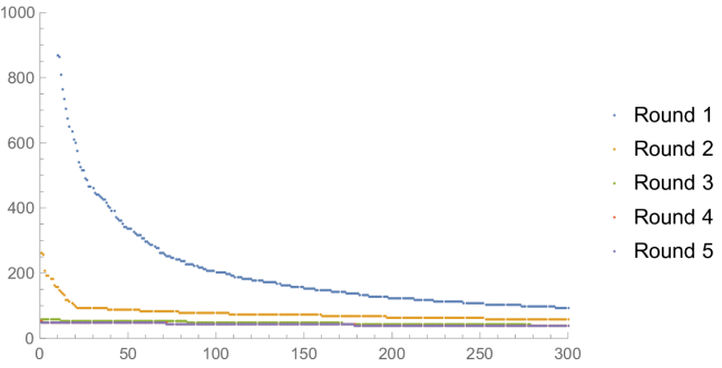
Figure 5: Histogram of frequency of appearance of 2-grams after 5 rounds of hyphenating the 2-grams with frequencies exceeding 50. We see that after 2 iterations the distribution is essentially flat, signifying that words which should be hyphenated have been.

In this Appendix, we describe the process and consequences of cleaning. We work with $120,249$ titles from hep-th, with a total of $996,485$ words, of which $48,984$ are unique. First, we convert the text to lower case and remove punctuation. Next, after replacing plurals, foreign spellings and some technical acronyms (such as “ramond ramond” $\to$ “rr”), we are left with $701,794$ words of which $32,693$ are unique.

Now, we can let the computer find the most common $2$-grams (words which appear adjacent to each other). The top hits are “gauge theory”, “field theory”, “scalar field”, etc. These terms are collective nouns. They clearly need to be hyphenated and considered as single words. Plotting the frequency of the top $300$ $2$-grams, one can see that there is a tailing off at around $50$ or so (cf. Figure 5). This means that we should simply hyphenate $2$-grams that appear more than $50$ times.

We repeat this process, hyphenating on each iteration those $2$-grams that appear with a frequency exceeding $50$. This can concatenate strings to form $3$-grams, such as the word “quantum-field-theory”. Figure 5 shows that the histogram becomes essentially flat after two iterations. This is quite interesting as it signifies that technical words which should be hyphenated can be detected automatically. We will use the flatness of the curve to stop the automatic replacements after two rounds of hyphenation. For reference, we record the most common ten words at each round of replacements, as well as the number of times that they appear.

Round 1	$\{\{\{$gauge, theory$\}$, 3232$\}$, $\{\{$field, theory$\}$, 2937$\}$, $\{\{$string, theory$\}$, 2025$\}$, $\{\{$quantum, gravity$\}$, 1552$\}$, $\{\{$yang-mills, theory$\}$, 1207$\}$, $\{\{$scalar, field$\}$, 1174$\}$, $\{\{$quantum, mechanics$\}$, 1117$\}$, $\{\{$dark, energy$\}$, 1084$\}$, $\{\{$matrix, model$\}$, 1040$\}$, $\{\{$cosmological, constant$\}$, 869$\}\}$
Round 2	$\{\{\{$string-field, theory$\}$, 260$\}$, $\{\{$susy-gauge, theory$\}$, 255$\}$, $\{\{$loop-quantum, gravity$\}$, 209$\}$, $\{\{$scalar-field, theory$\}$, 191$\}$, $\{\{$chiral-symmetry, breaking$\}$, 191$\}$, $\{\{$n=4-sym, theory$\}$, 182$\}$, $\{\{$lattice-gauge, theory$\}$, 182$\}$, $\{\{$topological-field, theory$\}$, 162$\}$, $\{\{$noncommutative-gauge, theory$\}$, 158$\}$, $\{\{$susy-quantum, mechanics$\}$, 155$\}\}$
Round 3	$\{\{\{$pair, creation$\}$, 56$\}$, $\{\{$cosmic, censorship$\}$, 56$\}$, $\{\{$holographic, principle$\}$, 56$\}$, $\{\{$three, dimensional$\}$, 56$\}$, $\{\{$logarithmic, correction$\}$, 56$\}$, $\{\{$dimensional, regularization$\}$, 56$\}$, $\{\{$nonlinear, susy$\}$, 56$\}$, $\{\{$susy, standard-model$\}$, 56$\}$, $\{\{$stochastic, quantization$\}$, 56$\}$, $\{\{$density, perturbation$\}$, 56$\}\}$
Round 4	$\{\{\{$heavy-ion, collisions$\}$, 52$\}$, $\{\{$new, massive-gravity$\}$, 49$\}$, $\{\{$conformal, algebra$\}$, 49$\}$, $\{\{$warped, compactification$\}$, 49$\}$, $\{\{$group, manifold$\}$, 49$\}$, $\{\{$weak, gravity$\}$, 49$\}$, $\{\{$stress-energy, tensor$\}$, 49$\}$, $\{\{$elementary, particle$\}$, 49$\}$, $\{\{$bose, gas$\}$, 49$\}$, $\{\{$new, results$\}$, 49$\}\}$
Round 5	$\{\{\{$new, massive-gravity$\}$, 49$\}$, $\{\{$conformal, algebra$\}$, 49$\}$, $\{\{$warped, compactification$\}$, 49$\}$, $\{\{$group, manifold$\}$, 49$\}$, $\{\{$weak, gravity$\}$, 49$\}$, $\{\{$stress-energy, tensor$\}$, 49$\}$, $\{\{$elementary, particle$\}$, 49$\}$, $\{\{$bose, gas$\}$, 49$\}$, $\{\{$new, results$\}$, 49$\}$, $\{\{$brownian, motion$\}$, 49$\}\}$

Appendix B Higher $n$-Grams across the Sections

In this appendix, we will present some statistic of the higher $n$-grams for the various arXiv sections, extending the 1-gram (words) and 2-gram analyses in Sections 5.1 and 5.2. The $15$ most common $3$-grams in hep-th titles are: Raw {{quantum,field,theory},826}, {{a,note,on},620}, {{conformal,field,theory},477}, {{in,string,theory},475}, {{string,field,theory},399}, {{the,cosmological,constant},395}, {{at,finite,temperature},390}, {{the,presence,of},353}, {{in,the,presence},346}, {{the,standard,model},329}, {{conformal,field,theories},324}, {{field,theory,and},284}, {{in,de,sitter},281}, {{approach,to,the},273}, {{corrections,to,the},263} Cleaned {{weak,gravity,conjecture},41}, {{causal,dynamical,triangulations},37}, {{strong,cp,problem},30}, {{string,gas,cosmology},29}, {{van,der,waals},28}, {{ads$\_$5,times,s^∧5},25}, {{shape,invariant,potential},24}, {{chern-simons,matter,theory},24}, {{ads/cft,integrability,chapter},23}, {{review,ads/cft,integrability,},23}, {{type,0,string-theory},23}, {{closed,timelike,curves},22}, {{hard,thermal,loop},22}, {{lowest,landau,level},22}, {{varying,speed,light},21}

Once again, more information is to be found in the cleaned $3$-grams. We conclude here as well that the most common terms such as “weak gravity conjecture”, “causal dynamical triangulations”, or “the strong CP problem” should be collective nouns with more stringent cleaning.

Finally, the $15$ most common $4$-grams in hep-th titles are: Raw {{in,the,presence,of},345}, {{in,quantum,field,theory},201}, {{a,note,on,the},181}, {{and,the,cosmological,constant},145}, {{the,cosmological,constant,problem},120}, {{in,de,sitter,space},111}, {{of,the,standard,model},94}, {{open,string,field,theory},89}, {{the,presence,of,a},89}, {{in,conformal,field,theory},82}, {{chiral,symmetry,breaking,in},81}, {{in,a,magnetic,field},81}, {{of,the,cosmological,constant},80}, {{effective,field,theory,of},80}, {{the,moduli,space,of},77} Cleaned {{review,ads/cft,integrability,chapter},23}, {{solution,strong,cp,problem},12}, {{chiral,de,rham,complex},9}, {{superstring,derived,standard-like,model},8}, {{bundle,formulation,nonrelativistic-quantum,mechanics},7}, {{fibre,bundle,formulation,nonrelativistic-quantum},7}, {{radiatively,induced,lorentz,cpt-violation},7}, {{vortex,model,ir,sector},7}, {{center,vortex,model,ir},7}, {{ultra,high-energy,cosmic,rays},7}, {{radiation,d-dimensional,collision,shock-wave},7}, {{5d,standing,wave,braneworld},7}, {{logarithmic,tensor,category,theory,},7}, {{five-dimensional,tangent,vector,spacetime},7}, {{shear-viscosity,entropy,density,ratio},7}

The most common cleaned $4$-gram is a reference to the Beisert, et al. review on the integrable structure of ${\cal N}=4$ super-Yang–Mills theory [45]. While again certain $4$-grams obviously point to “a solution to the strong CP problem” or “the chiral de Rham complex”, the prevalence of these terms are sufficiently scarce in the database that finding these collective terms automatically is somewhat difficult. What is striking as a member of the hep-th community is that these collective nouns tie in nicely to an expert’s conception of what it is that hep-th people do.

In analogy to Figure 3, we consider in Table 16 word clouds based on cleaned data for the subjects hep-ph, hep-lat, gr-qc, and math-ph. An expert can associate any of these word clouds with the label of the corresponding subject area. Thus, it is not entirely surprising that machine learning algorithms can discriminate titles between these areas as well.

A paper may be of interest to readers of the arXiv in more than one subject area and indeed, can reasonably be posted in either of hep-th or hep-ph, for example. Cross-listing on the arXiv enlarges the readership of a paper and enables the expression of a diversity of scientific interests. For these reasons, there is a significant overlap between the terms that appear in the word clouds. The emphasis of certain themes, however, renders the identification unambiguous.

	# Papers	# Unique Words	Word Cloud		# Papers	# Unique Words	Word Cloud
hep-ph	133,346	46,011		hep-lat	21,123	10,639
gr-qc	69,386	26,222		math-ph	51,747	28,559

Table 16: Some simple statistics of all titles of the various sections of the high energy arXiv, from the beginning in 1990 until 2017. The titles are cleaned according do the discussions in Section 3.2. The word cloud is sized according to frequency of relevant words. The number of papers and associated number of total unique words were compiled in December 2017.

The most common $15$ $3$-grams in the other arXiv sections based on cleaned data are: hep-ph {hidden,local,symmetry}, {hadron,resonance,gas}, {hard,thermal,loop}, {fine,structure,constant}, {higgs,triplet,model}, {t,bar,t}, {hadronic,light-by-light,scattering}, {resonance,gas,model}, {delta,i=1/2,rule}, {inverse,magnetic,catalysis}, {large,momentum,transfer}, {active,galactic,nuclei}, {susy,flavor,problem}, {q,bar,q}, {future,lepton,colliders} hep-lat {gluon,ghost,propagators}, {electric,dipole,moment}, {hadronic,vacuum,polarization}, {numerical,stochastic,perturbation-theory}, {mass,anomalous,dimension}, {first,order,phase-transition}, {maximum,entropy,method}, {causal,dynamical,triangulations}, {matrix,product,state}, {hadron,resonance,gas}, {chiral,magnetic,effect}, {delta,i=1/2,rule}, {physical,pion,mass}, {neutron,electric,dipole}, {nucleon,axial,charge} gr-qc {matters,gravity,newsletter}, {einstein,static,universe}, {causal,dynamical,triangulations}, {initial,value,problem}, {modified,newtonian,dynamics}, {topical,group,gravitation}, {van,der,waals}, {eddington-inspired,born-infeld,gravity}, {crossing,phantom,divide}, {baryon,acoustic,oscillation}, {physical,society,volume}, {american,physical,society,}, {newsletter,topical,group}, {gravity,newsletter,topical}, {lunar,laser,ranging} math-ph {asymmetric,simple-exclusion,process}, {spectruml,shift,function}, {alternating,sign,matrix}, {mutually,unbiased,bases}, {shape,invariant,potential}, {space,constant,curvature}, {quantum,affine,algebra}, {quantum,dynamical,semigroup}, {density,functional,theory}, {position,dependent,mass}, {inverse-scattering,fixed,energy}, {random,band,matrix}, {random,energy,model}, {asymptotic,iteration,method}, {spin,glass,model}

Finally, the $15$ most common $4$-grams in the other arXiv sections based on cleaned data are:

hep-ph	{hadron,resonance,gas,model}, {variation,fine,structure,constant}, {35,kev,x-ray,line}, {au+au,collision,sqrts$\_$nn=200,gev}, {130,gev,gamma-ray,line}, {hadronic,light-by-light,scattering,muon-g-2}, {hadronic,light-by-light,scattering,contribution}, {weak,radiative,hyperon,decay}, {after,lhc,run,1}, {nambu,-,jona-lasinio,model}, {variable,flavor,number,scheme}, {large,hadron,electron,collider}, {fermi,large,area,telescope}, {flavor,asymmetry,nucleon,sea}, {mu,-$>$,e,gamma}
hep-lat	{neutron,electric,dipole,moment}, {ground,state,entropy,potts}, {center-vortex,model,ir,sector}, {hadron,resonance,gas,model}, {i=2,pion,scattering,length}, {gluon,ghost,propagators,landau-gauge}, {higgs,boson,mass,bound}, {international,lattice,data,grid}, {landau-gauge,gluon,ghost,propagators}, {color,confinement,dual,superconductivity}, {state,entropy,potts,antiferromagnets}, {hadronic,contribution,muon,g-2}, {nearly,physical,pion,mass}, {weinberg,-,salam,model}, {kaon,mixing,beyond,sm}
gr-qc	{american,physical,society,volume}, {newsletter,topical,group,gravitation}, {gravity,newsletter,topical,group}, {matters,gravity,newsletter,topical}, {group,gravitation,american,physical}, {topical,group,gravitation,american}, {gravitation,american,physical,society,}, {matters,gravity,newsletter,aps}, {innermost,stable,circular,orbit}, {stability,einstein,static,universe}, {newsletter,aps,topical,group}, {gravity,newsletter,aps,topical}, {space,affine,connection,metric}, {instanton,representation,plebanski,gravity}, {laser,astrometric,test,relativity}
math-ph	{mean-field,spin,glass,model}, {long,range,scattering,modified}, {deformation,expression,elements,algebra}, {totally,asymmetric,simple-exclusion,process}, {nonlinear,accelerator,problems,wavelets}, {scattering,modified,wave,operator}, {range,scattering,modified,wave}, {spectruml,parameter,power,series}, {matrix,schrodinger-operator,half,line}, {five-dimensional,tangent,vector,spacetime}, {causal,signal,transmission,quantum-field}, {master,constraint,programme,lqg}, {set,spin,values,cayley-tree}, {uncountable,set,spin,values}, {model,uncountable,set,spin}

References

- [1] https://arxiv.org.
- [2] P. Ginsparg, “It was twenty years ago today…,” https://arxiv.org/abs/1108.2700 (2011).
- [3] https://arxiv.org/help/stats/2017_by_area/index (2018).
- [4] A. Plume and D. Van Weijen, “Publish or perish? The rise of the fractional author?,” Research trends 38, 16 (2014).
- [5] F. Denef, “Thoughts on future landscapes,” Northeastern lecture (2017).
- [6] V. Voevodsky, “Type systems and proof assistant,” IAS lecture (2012).
- [7] M. Ganesalingam and W. T. Gowers, “A fully automatic problem solver with human-style output,” arXiv:1309.4501 (2013).
- [8] Machine Learning in Physics, https://physicsml.github.io/pages/papers.html
-
[9]
Y. H. He,
“Deep learning the landscape,”
arXiv:1706.02714 [hep-th].
–, “Machine learning the string landscape,” Phys. Lett. B 774, 564 (2017). doi:10.1016/j.physletb.2017.10.024 - [10] F. Ruehle, “Evolving neural networks with genetic algorithms to study the string landscape,” JHEP 1708, 038 (2017) [arXiv:1706.07024 [hep-th]].
- [11] J. Carifio, J. Halverson, D. Krioukov, and B. D. Nelson, “Machine learning in the string landscape,” JHEP 1709, 157 (2017) [arXiv:1707.00655 [hep-th]].
- [12] J. Carifio, W. J. Cunningham, J. Halverson, D. Krioukov, C. Long and B. D. Nelson, “Vacuum Selection from Cosmology on Networks of String Geometries,” arXiv:1711.06685 [hep-th].
- [13] D. Krefl and R. K. Seong, “Machine learning of Calabi–Yau volumes,” Phys. Rev. D 96, no. 6, 066014 (2017) [arXiv:1706.03346 [hep-th]].
- [14] Y. N. Wang and Z. Zhang, “Learning non-Higgsable gauge groups in 4D F-theory,” arXiv:1804.07296 [hep-th].
- [15] K. Bull, Y. H. He, V. Jejjala and C. Mishra, arXiv:1806.03121 [hep-th].
-
[16]
Evert van Nieuwenburg, “Machine learning the arXiv”,
https://quantumfrontiers.com/2017/11/29/machine-learning-the-arxiv/
cf. Physics2Vec: http://everthemore.pythonanywhere.com/ - [17] T. Mikolov, K. Chen, G. Corrado, and J. Dean, “Efficient estimation of word representations in vector space,” arXiv:1301.3781 (2013).
- [18] T. Mikolov, I. Sutskever, K. Chen, G. Corrado, and J. Dean, “Distributed representations of words and phrases and their compositionality,” arXiv:1301.3781 (2013).
- [19] R. Řehůřek and P. Sojka, “Software framework for topic modelling with large corpora,” Proceedings of the LREC 2010 Workshop on New Challenges for NLP Frameworks, ELRA, 2010, https://radimrehurek.com/gensim/index.html
- [20] Paul Ginsparg, Paul Houle, Thorsten Joachims, Jae-Hoon Su, “Mapping Subsets of Scholarly Information”, arXiv:cs/0312018 [cs.IR]
- [21] HM Collins, P Ginsparg, L Reyes-Galindo, “A note concerning Primary Source Knowledge”, arXiv:1605.07228 [physics.soc-ph]
- [22] P. Ginsparg “Preprint Déjà Vu: an FAQ”, arXiv:1706.04188 [cs.DL]
- [23] Alexander Alemi, “Zombies Reading Segmented Graphene Articles On The Arxiv”, https://ecommons.cornell.edu/handle/1813/40878
- [24] D. Mimno and L. Thompson, “The strange geometry of skip-gram with negative sampling”, Proceedings of the 2017 Conference on Empirical Methods in Natural Language Processing, 2873-2878, (2017).
- [25] Peter D. Turney, Patrick Pantel, “From Frequency to Meaning: Vector Space Models of Semantics” Journal of Artificial Intelligence Research 37 (2010) 141-188. http://www.jair.org/media/2934/live-2934-4846-jair.pdf
-
[26]
Kunal Jain,
“An Intuitive Understanding of Word Embeddings: From Count Vectors to Word2Vec”,
https://www.analyticsvidhya.com/blog/2017/06/word-embeddings-count-word2veec/
deeplearning4J team, “Word2Vec”, https://deeplearning4j.org/word2vec -
[27]
Tomas Mikolov, Kai Chen, Greg Corrado, Jeffrey Dean,
“Efficient Estimation of Word Representations in Vector Space”,
arXiv:1301.3781[cs.CL]
–, “Distributed Representations of Words and Phrases and their Compositionality”, arXiv:1310.4546 [cs.CL]
Y. Goldberg, O. Levy, “word2vec Explained: deriving Mikolov et al.’s negative-sampling word-embedding method”, arXiv:1402.3722 [cs.CL] - [28] E. Witten, “Ground ring of two-dimensional string theory,” Nucl. Phys. B 373, 187 (1992) doi:10.1016/0550-3213(92)90454-J [hep-th/9108004].
-
[29]
G. Cybenko, “Approximations by superpositions of sigmoidal functions”, Mathematics of Control, Signals, and Systems, 2 (4), 303-314, (1989),
Kurt Hornik, “Approximation Capabilities of Multilayer Feedforward Networks”, Neural Networks, 4(2), 251–257, (1991) . - [30] Stanford CS Course, “CS224d: Deep Learning for Natural Language Processing”, http://cs224d.stanford.edu/syllabus.html
- [31] Dimitrios Kartsaklis, Sanjaye Ramgoolam, Mehrnoosh Sadrzadeh, “Linguistic Matrix Theory”, arXiv:1703.10252 [cs.CL].
- [32] News Headlines Of India, 16 years of categorized headlines focusing on India, https://www.kaggle.com/therohk/india-headlines-news-dataset
- [33] A. Strominger, JHEP 1407, 152 (2014) [arXiv:1312.2229 [hep-th]].
-
[34]
Georgios Balikas, Massih-Reza Amini,
“An empirical study on large scale text classification with skip-gram embeddings”, arXiv:1606.06623 [cs.CL];
Matt Taddy, “Document Classification by Inversion of Distributed Language Representations,” in Proceedings of the 2015 Conference of the Association of Computational Linguistics cf. also http://www.davidsbatista.net/blog/2017/04/01/document_classification/ , https://stackoverflow.com/questions/47563821/how-can-i-use-word2vec-to-train-a-classifier
http://nadbordrozd.github.io/blog/2016/05/20/text-classification-with-word2vec/
https://datawarrior.wordpress.com/2016/10/12/ - [35] Ian Goodfellow, Yoshua Bengio and Aaron Courville, “Deep Learning”, MIT Press, 2016, http://www.deeplearningbook.org
- [36] Wikipedia, https://www.wikipedia.org
- [37] Yahoo! Answers, https://answers.yahoo.com
-
[38]
Xiang Zhang and Yann LeCun, “Text Understanding from Scratch”, arXiv:1502.01710;
Xiang Zhang, Junbo Jake Zhao and Yann LeCun, “Character-level Convolutional Networks for Text Classification”, arXiv:1509.01626. - [39] The snarxiv, http://snarxiv.org/
- [40] David Simmons-Duffin, “The arXiv According to arXiv vs. snarXiv”, http://davidsd.org/2010/09/the-arxiv-according-to-arxiv-vs-snarxiv/
- [41] ‘An alternative archive e-prints in Science and Mathematics serving the whole scientific community’, http://vixra.org/
- [42] L. Leydesdorff and S. Milojevic, “Scientometrics,” arXiv:1208.4566 [cs.CL].
- [43] “Big Data Visualization of the Week: Paperscape,” Inside BIGDATA, October 22, 2013; http://blog.paperscape.org.
- [44] Quoc Le, Tomas Mikolov “Distributed Representations of Sentences and Documents”, https://cs.stanford.edu/~quocle/paragraph_vector.pdf
- [45] N. Beisert et al., “Review of AdS/CFT Integrability: An Overview,” Lett. Math. Phys. 99, 3 (2012). [arXiv:1012.3982 [hep-th]].