Cosmology of the interacting Cubic Galileon

Abstract

We consider the cosmological dynamics of the cubic Galileon field model interacting with dark matter, where the interaction between the cosmic dark sectors is proportional to Hubble parameter and dark energy density. The background field equations are converted into an autonomous dynamical system of first order equations using suitable dimensionless variables. The fixed points are determined and their stability analyzed by means of the eigenvalue method. The analysis of the stability of the fixed points along that of the avoidance of ghosts and Laplacias instabilities implies negative coupling parameter. We find an attractor fixed point in the de Sitter phase, and construct an approximated tracker solution, which to a good approximation, mimics the background cosmic evolution obtained by solving numerically the autonomous system of equations. In addition, we perform the statefinder and $Om$ diagnostics and show that for some appropriate values of the coupling constant and initial conditions, the trajectories in the statefinder parameter phase space evolves towards a stable state corresponding to $\Lambda\textrm{CDM}$ model. The comparison with the observed distance modulus and Hubble parameter data sets clearly indicates that the cosmological dynamics of the interacting cubic model is compatible with the existence of an interaction between the dark sectors.

1 Introduction

In recent years, the great amount with increasing precision of cosmological observations test of the standard $\Lambda\textrm{CDM}$ cosmological model strongly indicate the existence of non-baryonic cold dark matter (CDM), and that the present universe is in an epoch of accelerated expansion with redshift $z\lesssim 1$ [1, 2, 3, 4, 5, 6, 7]. Among many other puzzling problems in $\Lambda\textrm{CDM}$ model, the recent accelerated expansion of the universe, known as the late-time acceleration, constitute one of the greatest challenges of modern cosmology. Many extensions of general relativity have been explored to alleviate this problem. Given that matter with positive pressure generates deccelerated expansion, cosmologists suggested that the late-time acceleration of the universe is sourced by an exotic energy component with negative pressure, known as dark energy (DE) [8, 9, 10, 11]. One of the simplest and earliest candidate of DE, frequently invoked, is the cosmological constant $\Lambda$. Even though this model fits very well the cosmological observations, it is plagued several drawbacks, like fine tuning and coincidence problem [12]. The first one, known as the cosmological constant problem, is related to the large discrepancy between the theoretical value of $\Lambda$ predicted by quantum field theories and its observed value [13]. The coincidence problem asks the question, “Why are the densities of non relativistic matter and vacuum of the same order precisely today ?”, even though they evolve differently. These problems have led to increased interest in models where general relativity is modified in a way to alleviate the mentioned problems and produce the observed late time acceleration without generating new drawbacks. A plethora of theoretical models have been proposed to solve the mentioned problems. Two ways have been borrowed, the first one consists in modeling the right hand side of Einstein’s equations with specific forms of energy-momentum tensor containing the new exotic energy component with negative pressure, and an equation of state parameter, $w_{\textrm{de}}<-1/3$. If the equation of state is not just a constant, the fine tuning problem usually plaguing DE models with constant equation of state, can be avoided. An important class of DE models having this property are scalar quintessence field [14, 15, 16, 17, 18, 19], where the quintessence field couples minimally to gravity and is a dynamical slowly evolving component with negative pressure, and its equation of state is no longer constant but slightly evolves with time. It behaves like a cosmological constant, $\omega\approx-1$, if the potential term dominates over the kinetic term and thus generates sufficient negative pressure to drive the late time acceleration. However, attempts to resolve the coincidence problem are faced with fine tuning of the model parameters. Another variety of scalar field DE models has been proposed including k-essence [20], and tachyons fields [21, 22] and Chaplygin gaz [23, 24].

Because of the infeasibility of solving such theoretical problems, cosmologists have started to look at the second approach, which tends to modify the left hand side of Einstein’s equation. This alternative approach postulates that general relativity is only accurate on small scales, and the laws of gravity fail to describe the universe at large scales, so it has to be modified. One of the best studied models in this approach is the 5-dimensional Dvali- Gabadadze-Parroti brane-world model (DGP) [25], in which matter is confined to the 4-dimensional brane and only gravity can propagate in the 5-dimensional bulk. The DGP model can be compatible with local gravity constraints. However, its self-accelerating solution contains a ghost mode [26, 27], in addition to being incompatible with the joint observational constraints of Supernovae Ia (SN Ia), Baryon Acoustic Oscillations (BAO) and Cosmic Microwave Background (CMB) anisotropies [28, 29, 30, 31, 32, 33]. In order to avoid the appearance of ghosts in DGP model, a solution to the large scale modification of gravity is provided by an effective scalar field $\pi$ dubbed Galileon, which appears in the decoupling limit of DGP model [34, 35], and satisfying the Galilean shift symmetry $\partial_{\mu}\pi\rightarrow\partial_{\mu}\pi+b_{\mu}$ on Minkowskian background. Nicolis et al. [26] showed that there are only five field Lagrangians $\mathcal{L}^{\left(i\right)}(i\ =\overline{1,5})$ that respect the Galilean symmetry in the Minkowski background. In Refs. [36, 37] these Lagrangians have been extended to covariant forms in curved space-time while keeping the equations of motion up to second order. Consequently, this property allows to avoid the appearance of extra unphysical degenerated modes associated with ghosts, while the late-time cosmic acceleration can be realized by the field kinetic energy [38, 39, 40, 41, 42, 43, 44, 45, 47, 46]. There exists also another class of theories of large scale modification of gravity. These are known as $f(R)$ gravity, where $f$ is a function of Ricci scalar [48, 49, 50, 51]. Although such theories are able to describe the recent late-time accelerated expansion on cosmological scales correctly, they typically give rise to strong effects on local scales. Other models in the same context are scalar-tensor theories [52, 53, 54, 55, 56, 57], and Gauss-Bonnet gravity [58, 59]. An attractive feature of these models is that the cosmic late-time acceleration can be realized without recourse to an exotic energy component.

Finally, a third way to solve the drawbacks of the standard $\Lambda\textrm{CDM model}$ has emerged some times ago and several authors have invoked the possibility, that DE might directly interact with DM by exchanging energy during their cosmic evolution. Originally, this approach was used to explain the smallness of the cosmological constant [60, 61], and has become a fruitful framework to solve the coincidence problem [62, 63, 64, 65, 66, 67, 68, 69, 70, 71, 72, 73, 74, 75, 76]. An other motivation of introducing an interaction between the cosmic dark sectors is to improve the prediction of the standard cosmological model concerning the structures formation and their evolution. Inspired by string theories and scalar-tensor theories, several authors studied interaction between quintessence field and dark matter [77, 78]. Despite the lack of a fundamental theory for the interaction between dark sectors, a plethora of phenomenological forms of the interaction term have been proposed and constrained by observations (see e.g. [79] and references therein). Recently in [80], it has been find that DE-DM interaction alleviate the current tension between the value $H_{0}$ constrained from the Planck Cosmic Microwave Background measurement [81] and the recent estimate of Riess et al.[82].

In the present work, we study the cosmological effects of DE-DM interaction in the framework of the Galileon model. This paper is organized as follows. In section 2 we present a short review of the cubic Galileon field model and derive the field equations on general space-time. In section 3 we introduce the DE-DM interaction term into the cubic Galileon model and obtain the background field equations on spatially flat Friedmann-Lemaitre-Robertson-Walker (FLRW) space-time. Assuming the existence of de Sitter (dS) stable epoch and exploiting its cosmological properties, we reduce the dimension of the model parameter space. In section 4 using suitable dimensionless dynamical variables the field equations are converted into an autonomous system of first order differential equations. The later are solved and the fixed points determined and their stability analyzed. In 5, the conditions for the avoidance of ghosts and Laplacian instabilities are established. In section 6 we analyze in detail the cosmological evolution of the background parameters in the eras governed by the fixed points, along with the no-ghost and absence of Laplacian instabilities conditions, and derive appropriate constraints on DE-DM coupling constant. We also show the existence of a stable dS epoch and construct a approximate tracking solution. In section 7 the detailled numerical integration of the model is performed for the exact solution and the approximated tracking solutions. The cosmological behavior is also investigated using the statefinder and $Om$ diagnostics. Finally, conclusions are drawn in in Section 8.

2 Cubic Galileon model

Let us start with the action of the cubic Galileon field model as given in [36, 37]

$$S=\int d^{4}x\sqrt{-g}\left(\frac{M_{\textrm{Pl}}^{2}R}{2}+\frac{1}{2}\sum_{i=1}^{3}c_{i}\mathcal{L}^{\left(i\right)}\left[g_{\mu\nu},\pi\right]+\mathcal{L}_{M}\left[g_{\mu\nu},\left\{\phi_{a}\right\}\right]\right)$$ (2.1)

where $M_{\textrm{Pl}}^{2}$ is the reduced Planck mass related to Newton’s constant $M_{\textrm{Pl}}^{2}=1/8\pi G$, $g$ the determinant of the metric tensor $g_{\mu\nu}$, $R$ the Ricci scalar, $c_{i}$ are constants parameters, $\mathcal{L}^{\left(i\right)}$ are the Lagrangians for the Galileon field $\pi$ assumed to be minimally coupled to the metric, and $\mathcal{L}_{M}$ is the sum of radiation, baryonic and dark matter contributions with a set of fields $\left\{\phi_{a}\right\}$. In this model the Galileon is considered as the source of dark energy. The Lagrangians of interest are given by

$$\mathcal{L}^{\left(1\right)}=M^{3}\pi,\quad\mathcal{L}^{\left(2\right)}=\left(\nabla\pi\right)^{2}=\pi_{;\mu}\pi^{;\mu},\quad\mathcal{L}^{\left(3\right)}=\frac{1}{M^{3}}\left(\nabla\pi\right)^{2}\square\pi.$$ (2.2)

As we can see, $\mathcal{L}^{\left(1\right)}$ is a linear potential for the Galileon , $\mathcal{L}^{\left(2\right)}$ the standard quadratic kinetic Lagrangian, and $\mathcal{L}^{\left(3\right)}$ the cubic Lagrangian which arises in the decoupling limit of the DGP model [34, 35]. In addition, $M$ is a constant with dimension of mass, such that $M^{3}=$$M_{\textrm{Pl}}H_{\textrm{dS}}^{2}$ and $H_{\textrm{dS}}$ being the Hubble expansion rate in the de Sitter (dS) epoch. If we set $c_{3}=0$ we have the standard quintessence Lagrangian.

The Einstein equations of motion derived by varying the action (2.1) with respect to $g_{\mu\nu}$ read

$$M_{\textrm{Pl}}^{2}G_{\alpha\beta}=T_{\alpha\beta},$$ (2.3)

where $G_{\alpha\beta}$ denotes the Einstein symmetric tensor, $T_{\alpha\beta}=\sum_{i=1}^{3}c_{i}T_{\alpha\beta}^{\left(i\right)}+\sum_{a}T_{\alpha\beta}^{\left(a\right)}$ is the total energy-momentum tensor where $T_{\alpha\beta}^{\left(i\right)}$ is the energy-momentum tensor of the Galileon field and $T_{\alpha\beta}^{\left(a\right)}$ the energy-momentum tensor of radiation, baryonic matter and dark matter $\left(a=\textrm{r,\>b\>,dm}\right)$. Starting from the relation

$$T_{\alpha\beta}^{\left(i\right)}=-\frac{2}{\sqrt{-g}}\frac{\delta S^{\left(i\right)}}{\delta g^{\alpha\beta}},\quad S^{\left(i\right)}=\int d^{4}x\sqrt{-g}\mathcal{L}^{\left(i\right)}\text{ }.$$ (2.4)

we easily show that

$$T_{\alpha\beta}^{\left(1\right)}=M^{3}\pi g_{\alpha\beta}\text{ },$$ (2.5)

$$T_{\alpha\beta}^{\left(2\right)}=-\pi_{;\alpha}\pi_{;\beta}+\frac{1}{2}g_{\alpha\beta}\left(\nabla\pi\right)^{2}\text{ },$$ (2.6)

$$T_{\alpha\beta}^{\left(3\right)}=-\frac{1}{M^{3}}\left(\pi_{;\alpha}\pi_{:\beta}\square\pi+g_{\alpha\beta}\pi_{;\mu}\pi^{;\mu\lambda}\pi_{;\lambda}-\pi^{;\mu}\left[\pi_{;\alpha}\pi_{;\beta\mu}+\pi_{;\beta}\pi_{;\alpha\mu}\right]\right).$$ (2.7)

For matter components, we assume the usual energy-momentum tensor describing a perfect fluid

$$T_{\alpha\beta}^{\left(i\right)}=\left(\rho_{i}+p_{i}\right)u_{\alpha}u_{\beta}+p_{i}g_{\alpha\beta}$$ (2.8)

where $\rho_{i}$ is the energy density, $p_{i}$ the pressure, and $u_{\alpha}$ the velocity of the fluid. We define also an Equation of State parameter (EoS) for each component in the form $p_{i}=w_{i}\rho_{i}.$ For radiation and pressurless mater (baryonic and cold dark matters) we have $w_{r}=1/3$ and $w_{b}=w_{dm}=0,$ respectively. In order to preserve the local energy-momentum conservation law, we have the conservation law

$$\nabla_{\alpha}T^{\alpha\beta}=0.$$ (2.9)

Finally, varying the action with respect to the Galileon field we obtain the equation of motion

$$\frac{c_{1}M^{3}}{2}-c_{2}\square\pi-\frac{c_{3}}{M^{3}}\left[\left(\square\pi\right)^{2}-R_{\mu\nu}\pi^{;\mu}\pi^{;\nu}-\pi_{;\mu\nu}^{2}\right]=0.$$ (2.10)

3 Background dynamics

In order to study the cosmological consequences of the interacting cubic Galileon, we assume the geometry of spatially flat expanding universe described by the FLRW metric

$$ds^{2}=-n^{2}\left(t\right)dt^{2}+a^{2}(t)\delta_{ij}dx^{\text{i}}dx^{j}$$ (3.1)

where $a\left(t\right)$ is the scale factor. Using $n^{2}\left(t\right)=1,$ the Friedmann equations on the FLRW background are obtained from the $(0,0)$ and $(i,j)$ components of Einstein equations ($\ref{ten2})$

$$3M_{\textrm{Pl}}^{2}H^{2}=-\frac{1}{2}c_{1}M^{3}\pi-\frac{1}{2}c_{2}\dot{\pi}^{2}+\frac{3}{M^{3}}c_{3}H\dot{\pi}^{3}+\rho_{\textrm{dm}}+\rho_{\textrm{b}}+\rho_{\textrm{r}}\text{ },$$ (3.2)

$$M_{\textrm{Pl}}^{2}(3H^{2}+2\dot{H})=-\frac{1}{2}c_{1}M^{3}\pi+\frac{1}{2}c_{2}\dot{\pi}^{2}+\frac{1}{M^{3}}c_{3}\dot{\pi}^{2}\ddot{\pi}-\frac{1}{3}\rho_{\textrm{r}}\text{ ,}$$ (3.3)

where $H=\frac{\dot{a}}{a}$ is the Hubble expansion rate, and a dot denote derivative with respect to time. From Friedmann equations (3.2) and (3.3), we identify the effective dark energy density and pressure of the Galileon field

$$\rho_{\pi}=-\frac{1}{2}c_{2}\dot{\pi}^{2}+\frac{3}{M^{3}}c_{3}H\dot{\pi}^{3},$$ (3.4)

$$P_{\pi}=-\frac{1}{2}c_{2}\dot{\pi}^{2}-\frac{1}{M^{3}}c_{3}\dot{\pi}^{2}\ddot{\pi}.$$ (3.5)

In the following we are interested by a late-time cosmic exapnsion acceleration realized by the field kinetic energy, such that we set $c_{1}=0$ in the rest of this paper. The Galileon field equation on the FLRW background is then given by

$$c_{2}M_{\textrm{Pl}}H_{\textrm{d}S}\left(\dot{\pi}H\left(\alpha-6\right)-2\ddot{\pi}\right)+c_{3}\left(6\dot{\pi}^{2}H^{2}\left(\alpha-3\right)-6\dot{\pi}^{2}\dot{H}-12\dot{\pi}\ddot{\pi}H\right)=0$$ (3.6)

In order to study the cubic Galileon model in its generality and make room to the existence of an energy transfer between DE and DM fields as supported by the observation of galaxy clusters [84, 85], we assume that the dark sector components do not evolve separately but interact with each other. The general way to describe this interaction is to introduce an energy-momentum exchange term into the conservation equations as follows

$$\nabla_{\alpha}T_{\textrm{de}}^{\alpha\beta}=-\nabla_{\alpha}T_{\textrm{dm}}^{\alpha\beta}=Q^{\beta}.$$ (3.7)

where $Q^{\beta}$ is given covariantly by [83]

$$Q_{\textrm{de/dm}}^{\beta}=Qu^{\beta},$$ (3.8)

and $u^{\beta}$ is the DE/DM 4-velocity. The function $Q,$ known as the interaction function between DE and DM, is generally function of DE and DM densities, Hubble parameter and its derivatives. Assuming that there is only energy transfer between DE and DM we have $Q_{\textrm{de}}=Q_{\textrm{dm}}=-Q.$ We mention that negative $Q$ indicates that DE decays to DM, whereas DM decays to DE for positive $Q$. In the FLRW space-time, Eq.(3.7) gives

$$\dot{\rho}_{de}+3H\left(\rho_{de}+P_{de}\right)=Q,$$ (3.9)

$$\dot{\rho}_{\textrm{dm}}+3H\rho_{\textrm{dm}}=-Q.$$ (3.10)

Once a form of $Q$ is given, the background dynamics is fully determined by the modified energy conservation equations (3.9) and (3.10) and the Friedmann equations (3.2) and (3.3). Additionally, the conservation laws for radiation and baryonic components on the FLRW background read

$$\dot{\rho}_{\textrm{r}}+4H\rho_{\textrm{r}}=0.$$ (3.11)

$$\dot{\rho}_{\textrm{b}}+H\rho_{\textrm{b}}=0.$$ (3.12)

At this stage let us take benefit from the existence of a dS background characterized by $H=H_{\textrm{dS}}\equiv cst$, $\dot{\pi}=\dot{\pi}_{\textrm{dS}}\equiv cst$, and fix the free parameters $c_{2},\>c_{3}$ in the Galileon Lagrangian in terms of the interaction function. Writing the Eqs. ($\ref{f1}),\>(\ref{f2}),\>(\ref{eq:field_equation})$ and ($\ref{eq:interaction})$ in the dS era, and solving the resulting equations we obtain

$$x_{\textrm{dS}}^{2}c_{2}=6,\quad x_{\textrm{dS}}^{3}c_{3}=\frac{18H_{\mathscr{\textrm{dS}}}^{3}M_{\textrm{Pl}}^{3}+Q_{\textrm{dS}}}{9H_{\mathscr{\textrm{dS}}}^{3}M_{\textrm{Pl}}^{3}}$$ (3.13)

$$\Omega_{\textrm{b},\textrm{dS}}=0,\quad\Omega_{\textrm{dm,dS}}=-\frac{Q_{\textrm{dS}}}{9H_{\textrm{dS}}^{3}M_{\textrm{Pl}}^{2}}.$$ (3.14)

where we have set $x_{\textrm{dS}}=\frac{\dot{\pi}_{\textrm{dS}}}{H_{\textrm{dS}}M_{\textrm{Pl}}}$ and normalized $M$ to $M^{3}=M_{\textrm{Pl}}H_{\textrm{dS}}^{2}$ (This give $M\approx 10^{-40}M_{\textrm{pl}}$ for $H_{\textrm{dS}}\approx 10^{-60}M_{\textrm{Pl}})$ [45]. This clearly shows that $Q_{\textrm{dS}}$ must be negative, signaling an energy transfer from DE to DM in the dS epoch. It is of interest to remark that the only relevant free parameters are the coupling parameters in the interaction function and that DM density in the dS era is not zero but depends on the the coupling parameters.

4 Generalized dynamical system

In this section, we study the cosmological dynamic of the interacting Galileon through the use of the autonomous dynamical systems and phase space trajectories analysis. The evolution equations (3.2) and (3.3 ) are first transformed to first order differential equations by the introduction of new dimensionless dynamical variables. To achieve this goal, we follow the analysis performed in the non-interacting case in [47, 45], and introduce the dimensionless variables $r_{1}$ and $r_{2}$

$$r_{1}=\frac{\dot{\pi}_{\textrm{dS}}H_{\textrm{dS}}}{\dot{\pi}H},\quad r_{2}=\frac{1}{r_{1}}\left(\frac{\dot{\pi}}{\dot{\pi}_{\textrm{dS}}}\right)^{4}.$$ (4.1)

From these definitions we easily obtain

$$\frac{H}{H_{\textrm{dS}}}=\frac{1}{r_{1}\left(r_{1}r_{2}\right)^{1/4}},\quad\frac{\dot{\pi}}{\dot{\pi}_{ds}}=\left(r_{1}r_{2}\right)^{1/4}.$$ (4.2)

In the dS phase, we have $r_{1}=1$ and $r_{2}=1.$ From Eqs. (3.11), (3.12) and (4.1) we easily obtain the following differential equations

$$r^{\prime}_{1}= -r_{1}\left(\frac{\ddot{\pi}}{\dot{\pi}H}+\frac{H^{\prime}}{H}\right),$$ (4.3)

$$r^{\prime}_{2}= r_{2}\left(\frac{\ddot{5\pi}}{\dot{\pi}H}+\frac{H^{\prime}}{H}\right),$$ (4.4)

$$\Omega^{\prime}_{\textrm{r}}= -2\Omega_{r}\left(2+\frac{H^{\prime}}{H}\right),$$ (4.5)

$$\Omega^{\prime}_{\textrm{b}}= -2\Omega_{b}\left(\frac{3}{2}+\frac{H^{\prime}}{H}\right),$$ (4.6)

where the prime indicates derivation with respect to $N=\ln a$, and the dimensionless energy density parameters are defined by

$$\Omega_{a}=\frac{\rho_{\textrm{a}}}{3M_{\textrm{Pl}}^{2}H^{2}},\quad\textrm{a}=\{\textrm{r,b,dm,de}\}.$$ (4.7)

The expression of dark energy density parameter $\Omega_{\textrm{de}}$ is now given in terms of $r_{1}$ and $r_{2}$ as

$$\Omega_{\textrm{de}} =-\frac{r_{1}^{2}r_{2}\left[\left(\alpha-3\right)r_{1}+6-\alpha\right]}{\alpha-3}.$$ (4.8)

Combining (4.3) and (4.4) we obtain the evolution equation of Hubble parameter

$$\frac{H^{\prime}}{H}=-\frac{5r_{1}^{\prime}}{4r_{1}}-\frac{r_{2}^{\prime}}{4r_{2}}.$$ (4.9)

Actually, it is impossible to derive the exact form of $Q$ from first principles, and the available forms are only on the basis of phenomenological considerations. Among the various interaction terms studied in the literature, we take in the present paper, the interaction function in the form

$$Q(\rho_{\textrm{dm}},\pi,\dot{\pi})=H\alpha\rho_{\textrm{de}}$$ (4.10)

where $\alpha$ is the constant coupling and $\alpha H$ is the rate of transfer of DE density. It is well known that this kind of interaction leads to stable linear perturbations with negative coupling constant. Then, Eqs.(3.13) and (3.14) reduce to

$$x_{\textrm{dS}}^{2}c_{2}=6,\quad x_{\textrm{dS}}^{3}c_{3}=\frac{\alpha-6}{\alpha-3},\quad\Omega_{\textrm{b},\textrm{dS}}=0,\quad\Omega_{\textrm{dm,dS}}=\frac{\alpha}{\alpha-3}.$$ (4.11)

The standard scenario in the non-interacting case is recovered for $\alpha=0$, and all the analysis performed above reduce to the one found in [45]. We now use (4.11) and rewrite (3.2) and (3.6) in terms of the dimensionless variables and solve in $\frac{H^{\prime}}{H}$ and $\frac{\ddot{\pi}}{\dot{\pi}H}$ to obtain

$$\frac{H^{\prime}}{H}= \left(\alpha-3\right)\frac{\Bigl{[}r_{1}^{2}r_{2}\left(r_{1}-1\right)\left(\alpha-6\right)^{2}+2\left(3r_{1}^{3}r_{2}-\Omega_{r}-3\right)\left(\alpha r_{1}-\alpha-3r_{1}+6\right)\Bigr{]}}{\Bigl{[}4\left(\alpha-3\right)\left(\alpha r_{1}-\alpha-3r_{1}+6\right)-r_{1}^{2}r_{2}\left(\alpha-6\right)^{2}\Bigr{]}},$$ (4.12)

$$\frac{\ddot{\pi}}{\dot{\pi}H}= \frac{\left(\alpha-3\right)\left(\alpha-6\right)\left[3r_{1}^{3}r_{2}-\Omega_{r}-3+2\left(\alpha-3\right)\left(r_{1}-1\right)\right]}{\Bigl{[}4\left(\alpha-3\right)\left[\alpha\left(r_{1}-1\right)-3r_{1}+6\right]-r_{1}^{2}r_{2}\left(\alpha-6\right)^{2}\Bigr{]}}.$$ (4.13)

Substituting in Eqs.(4.3)-(4.6), we obtain the following autonomous system of equations

$$r^{\prime}_{1}= \frac{r_{1}\left(\alpha-3\right)}{\Delta_{d}}\Bigl{[}\left(r_{1}^{3}r_{2}-r_{1}^{2}r_{2}+2\left(r_{1}-1\right)\right)\alpha^{2}$$

$$+\left(6r_{1}^{4}r_{2}-3r_{1}^{3}r_{2}+12r_{1}^{2}r_{2}-24r_{1}+\Omega_{r}\left(1-2r_{1}\right)+21\right)\alpha$$

$$-18\left(r_{1}^{2}-3r_{1}+2\right)r_{1}^{2}r_{2}+54\left(r_{1}-1\right)+6\Omega_{r}\left(r_{1}-1\right)\Bigr{]},$$ (4.14)

$$r_{2}^{\prime}=- \frac{r_{2}\left(\alpha-3\right)}{\Delta_{d}}\Bigl{[}\left(r_{1}^{3}r_{2}-r_{1}^{2}r_{2}+10\left(r_{1}-1\right)\right)\alpha^{2}$$

$$+\left(6r_{1}^{4}r_{2}-15r_{1}^{3}r_{2}+12r_{1}^{2}r_{2}-96r_{1}-\Omega_{r}\left(3+2r_{1}\right)+81\right)\alpha$$

$$-18\left(r_{1}^{2}+r_{1}+2\right)r_{1}^{2}r_{2}+18\left(11r_{1}-7\right)+6\Omega_{r}\left(r_{1}+2\right)\Bigr{]},$$ (4.15)

$$\Omega_{\textrm{r}}^{\prime}= \frac{2\Omega_{r}}{\Delta_{d}}\Bigl{[}\left(r_{1}-1\right)r_{1}^{2}r_{2}\alpha^{3}+\left(6r_{1}^{4}r_{2}-21r_{1}^{3}r_{2}+13r_{1}^{2}r_{2}-2\Omega_{r}\left(r_{1}-1\right)+2\left(r_{1}-1\right)\right)\alpha^{2}$$

$$+\left(-36r_{1}^{4}r_{2}+126r_{1}^{3}r_{2}-48r_{1}^{2}r_{2}+6\Omega_{r}\left(r_{1}-3\right)-6\left(r_{1}-3\right)\right)\alpha$$

$$+54r_{1}^{4}r_{2}-216r_{1}^{3}r_{2}+36r_{1}^{2}r_{2}-18\Omega_{r}\left(r_{1}-2\right)+18\left(r_{1}-2\right)\Bigr{]},$$ (4.16)

$$\Omega_{\textrm{b}}^{\prime}= \frac{\Omega_{b}}{\Delta_{d}}\Bigl{[}2\left(r_{1}-1\right)r_{1}^{2}r_{2}\alpha^{3}+\left(12r_{1}^{4}r_{2}-42r_{1}^{3}r_{2}+27r_{1}^{2}r_{2}-4\Omega_{r}\left(r_{1}-1\right)\right)\alpha^{2}$$

$$+\left(-36r_{1}^{4}r_{2}+126r_{1}^{3}r_{2}-48r_{1}^{2}r_{2}+12\Omega_{r}\left(r_{1}-1\right)-6\left(2r_{1}-3\right)\right)\alpha$$

$$+54r_{1}^{4}r_{2}-216r_{1}^{3}r_{2}+36r_{1}^{2}r_{2}-18\Omega_{r}\left(r_{1}-2\right)+18\left(r_{1}-2\right)\Bigr{]}$$ (4.17)

where $\Delta_{d}$ is given by

$$\Delta_{\textrm{d}}=\left(r_{1}^{2}r_{2}-4r_{1}+4\right)\alpha^{2}-12\left(r_{1}^{2}r_{2}-2r_{1}+3\right)\alpha+36\left(r_{1}^{2}r_{2}-r_{1}+2\right).$$ (4.18)

Now we express the dark energy EoS parameter $\omega_{\textrm{de}}=\frac{\rho_{\textrm{de}}}{P_{\textrm{de}}}$ and the total effective EoS parameter $\omega_{\textrm{eff}}=-1-\frac{2}{3}\frac{H^{\prime}}{H}$ in terms of the dynamical variables

$$w_{\textrm{de}}= -\frac{\left(\alpha-3\right)}{3\Delta_{\textrm{de}}}\left[\left(2r_{1}-2\right)\alpha^{3}+\left(12r_{1}^{2}-\Omega_{r}-42r_{1}+27\right)\alpha^{2}\right.$$

$$-\left(72r_{1}^{2}-12\Omega_{r}-252r_{1}+108\right)\alpha$$

$$\left.+108r_{1}^{2}-36\Omega_{r}-432r_{1}+108\right],$$ (4.19)

$$w_{\textrm{eff}}= \frac{1}{3\Delta_{\textrm{eff}}}\left[2r_{1}^{2}r_{2}\left(r_{1}-1\right)\alpha^{3}+\left[\left(12r_{1}^{2}-42r_{1}+27\right)r_{1}^{2}r_{2}-4\Omega_{r}\left(r_{1}-1\right)\right]\alpha^{2}\right.$$

$$-\left[\left(72r_{1}^{2}-252r_{1}+108\right)r_{1}^{2}r_{2}-12\Omega_{r}\left(2r_{1}-3\right)\right]\alpha$$

$$+\left.108\left(r_{1}^{2}-4r_{1}+1\right)r_{1}^{2}r_{2}-36\Omega_{r}\left(r_{1}-2\right)\right]$$ (4.20)

where

$$\Delta_{\textrm{eff}} =\left(r_{1}^{2}r_{2}-4r_{1}+4\right)\alpha^{2}-12\left(r_{1}^{2}r_{2}-2r_{1}+3\right)\alpha+36\left(r_{1}^{2}r_{2}-r_{1}+2\right),$$ (4.21)

$$\Delta_{\textrm{de}} =\Delta_{\textrm{eff}}\left(\left(r_{1}-1\right)\alpha-3r_{1}+6\right).$$ (4.22)

Let us denote the autonomous system (4.14)-(4.17) by

$$\dot{\vec{x}}=f\left(\overrightarrow{x}\right),\quad\overrightarrow{x}=\left(r_{1},r_{2},\Omega_{r},\Omega_{b}\right).$$ (4.23)

We proceed now to study the cosmological evolution of the interacting cubic Galileon model. We first determine the fixed or critical points of the dynamical system of equations and examine their stability during the cosmic history. The fixed points are the roots of equations $\dot{x}_{i}=0.$ The stability analysis is performed using first order perturbation technique around the fixed points and then form the matrix of coefficients of the perturbed terms. A fixed point is said stable (attractor) if the eigenvalues of the perturbation matrix are all negative, saddle if the eigenvalues are of mixed signs and unstable if the eigenvalues are all positive. We have found 5 fixed points, $A,\>B,\>C,\>D$ and $E$ and summarized their properties in Table.1, where $\mathcal{D}_{C}=\left[-\infty,-\frac{15+5\sqrt{17}}{2}\right[\cup\left]-\frac{15-5\sqrt{17}}{2},+\infty\right]$, $q=-1-\left(H^{\prime}/H\right)$ is the deceleration parameter, and

$$C_{\pm}=\frac{3\left(\alpha-3\right)}{2}\left[\frac{3\alpha-12\alpha+48\pm\alpha\sqrt{\left(3\alpha-20\right)\left(\alpha-12\right)}}{\alpha^{2}-24\alpha+72}\right].$$ (4.24)

Fixed Points	$\left(r_{1},\>r_{2}\>,\Omega_{r}\>,\Omega_{b}\right)$	Eigenvalues	Stability	q
A	$\left(0,0,1,0\right)$	$(1,1,\frac{5-\alpha}{2},-\frac{9-5\alpha}{2})$	$\begin{array}[]{c}\text{ Unst. }9/5<\alpha<5\text{, }\\ \text{Saddle otherwise}\end{array}$	$1$
B	$\left(0,0,0,\Omega_{b}\right)$	$(0,-1,\frac{9-2\alpha}{4},-\frac{21-10\alpha}{4})$	$\begin{array}[]{c}\text{ Unst. if }\alpha<5/2\text{, }\\ \text{Saddle otherwise}\end{array}$	$1/2$
C	$\left(\frac{\alpha^{2}-11\alpha+30}{\alpha^{2}-13\alpha+30},0,1,0\right)$	$(8,-\frac{\alpha^{2}}{10}+\frac{3\alpha}{2}-5,1,1)$	$\begin{array}[]{c}\text{ Unst. if }\alpha\in\mathcal{D}_{C}\\ \text{Saddle otherwise}\end{array}$	$1$
D	$\left(\frac{2\alpha^{2}-21\alpha+54}{2\alpha^{2}-24\alpha+54},\>0,\>0,\>\Omega_{b}\right)$	$(0,-1,6,-\frac{\alpha^{2}}{9}+\frac{3\alpha}{2}-\frac{9}{2})$	Saddle	$1$
E	$\left(1,1,0,0\right)$	$(-4,-3,\>C_{+},\>C_{-})$	$\begin{array}[]{c}\text{ Stable if }\alpha<3\text{, }\\ \text{Unst. otherwise}\end{array}$	$-1$

Table 1: Location, Eigenvalues and Stability of the Critical Points.

The two fixed points $A$ and $B$ are radiation and matter domination eras, respectively, with no contribution from dark energy. These points are unstable for $\alpha<5$ and $\alpha<9/2$, respectively. They constitute the so called small regime [45, 47]. The fixed point C and D are also pure radiation and matter dominated eras, respectively. They are unstable for $5<\alpha<10$ and $9/2<\alpha<9$, respectively. The last fixed point E is the dS point. It is stable if $\alpha<3$ and may plays the role of an attractor of the whole cosmological evolution, independently of the initial conditions on $r_{1},\,r_{2},\,\Omega_{r},\,\Omega_{b}$. We have two paths for a valid cosmological evolution. The first (second) path starts from the unstable dominated radiation era, A (C), continues toward unstable dominated matter era, B (D), and ends at the dS point, E. It is useful to note that, for $\alpha=0,$ all the dynamical analysis performed here reduce to the one in ref.[47], and the fixed points A, B, C, D become saddle points while de dS fixed point remains stable.

5 Ghosts and laplacian instabilities

In order to discuss the stability of theories described by the Lagrangian $(\ref{Action}$) in the cosmological context, a full treatment of the linear perturbation theory on the flat FLRW background has been presented in [45]. Accordingly, the conditions for the avoidance of ghosts and Laplacian instabilities have been determined. For the scalar modes the conditions are given by

$$Q_{\textrm{S}}\equiv\frac{\omega_{1}\left(4\omega_{1}\omega_{3}+9\omega_{2}^{2}\right)}{3\omega_{2}^{2}}>0,$$ (5.1)

$$C_{\textrm{S}}^{2}\equiv\frac{3\left(2\omega_{1}^{2}\omega_{2}H-\omega_{2}^{2}\omega_{4}+4\omega_{1}\omega_{2}\dot{\omega}_{1}-2\omega_{1}^{2}\dot{\omega}_{2}\right)-6\omega_{1}^{2}\left[\left(1+\omega_{r}\right)\rho_{r}+\left(1+\omega_{dm}\right)\rho_{dm}+\left(1+\omega_{b}\right)\rho_{b}\right]}{\omega_{1}(4\omega_{1}\omega_{3}+9\omega_{2}^{2})}\geqslant 0,$$ (5.2)

while the conditions on tensor modes are given by

$$Q_{\textrm{T}}\equiv\frac{\omega_{1}}{4}>0,\quad C_{\textrm{T}}^{2}\equiv\frac{\omega_{4}}{\omega_{1}}\geqslant 0$$ (5.3)

where $C_{\textrm{S}}^{2}$ and $C_{\textrm{T}}^{2}$ are the propagation speeds squared of scalar and tensor modes, respectively. In the interacting cubic Galileon model, the functions $\omega_{1},\>\omega_{2},\>\omega_{3}$ and $\omega_{4}$ read

$$\omega_{1}=M_{\textrm{Pl}}^{2},\quad\omega_{2}=-\frac{2c_{3}X\dot{\pi}}{M_{\textrm{Pl}}H_{\textrm{dS}}^{2}}+2M_{\textrm{Pl}}^{2}H,$$ (5.4)

$$\omega_{3}=-3c_{2}X+\frac{36c_{3}XH\dot{\pi}}{M_{\textrm{Pl}}H_{\textrm{dS}}^{2}}-9H^{2}M_{\textrm{Pl}}^{2},\quad\omega_{4}=M_{\textrm{Pl}}^{2},$$ (5.5)

where $X=-\frac{1}{2}\partial_{\mu}\pi\partial^{\mu}\pi$, and $c_{2}$ and $c_{3}$ given by (4.11). It is worth to note that the effect of the interaction between dark energy and dark matter is also encoded in the Hubble parameter. Expressed in terms of $r_{1}$and $r_{2}$, the functions $\omega_{2}$ and $\omega_{3}$ read

$$\omega_{2}=-\textrm{$M_{\textrm{Pl}}^{2}$}H_{\textrm{dS}}\left[\frac{\left(\alpha-6\right)r_{1}^{2}r_{2}-2\alpha+6}{\left(\alpha-3\right)r_{1}\left(r_{1}r_{2}\right)^{1/4}}\right],$$ (5.6)

$$\omega_{3}=-9M_{\textrm{Pl}}^{2}H_{\textrm{dS}}^{2}\left[\frac{\left(\alpha-3\right)\left(r_{1}^{3}r_{2}+1\right)-2\left(\alpha-6\right)r_{1}^{2}r_{2}}{\left(\alpha-3\right)r_{1}^{2}\left(r_{1}r_{2}\right)^{1/2}}\right].$$ (5.7)

Inserting Eqs. ($\ref{w1-2}),$ and ($\ref{w3-1})$ into Eqs. (5.1), (5.2), and (5.3), the conditions for the avoidance of ghosts and Laplacian instabilities for scalars and tensor modes become

$$Q_{\textrm{S}}= \frac{3\left[(r_{1}^{2}r_{2}-4r_{1}+4)\alpha^{2}-12(r_{1}^{2}r_{2}-2r_{1}+3)\alpha+36\left(r_{1}^{2}r_{2}-r_{1}+2\right)\right]r_{1}^{2}r_{2}}{\left[(\alpha-6)r_{1}^{2}r_{2}-2\alpha+6\right]^{2}},$$ (5.8)

$$C_{\textrm{S}}^{2}=-\frac{1}{3} \frac{N_{\textrm{S}}}{\left[(\alpha^{2}-12\alpha+36)r_{1}^{2}r_{2}-(4\alpha^{2}-24\alpha+36)r_{1}+4\alpha^{2}-36\alpha+72\right]^{2}},$$ (5.9)

$$Q_{\textrm{T}}= \frac{M_{\textrm{Pl}}^{2}}{4},\quad C_{\textrm{T}}^{2}=1.$$ (5.10)

where

$$N_{\textrm{S}} =\left(\alpha^{4}-24\alpha^{3}+216\alpha^{2}-864\alpha+1296\right)r_{1}^{4}r_{2}^{2}$$

$$+\left(20\alpha^{4}-360\alpha^{3}+2340\alpha^{2}-6480\alpha+6480\right)r_{1}^{5}r_{2}$$

$$+\left(-4\alpha^{4}+84\alpha^{3}-648\alpha^{2}+2160\alpha-2592\right)r_{1}^{2}r_{2}$$

$$+\left(-48\alpha^{4}+576\alpha^{3}-2592\alpha^{2}+5184\alpha-3888\right)r_{1}^{2}$$

$$+\left(8\alpha^{5}-88\alpha^{4}+168\alpha^{3}+1080\alpha^{2}-4752\alpha+5184\right)r_{1}$$

$$+\left(-4\alpha^{4}+72\alpha^{3}-468\alpha^{2}+1296\alpha-1296\right)\Omega_{r}$$

$$-8\alpha^{5}+124\alpha^{4}-576\alpha^{3}+252\alpha^{2}+3888\alpha-6480$$ (5.11)

It is useful to note that the conditions on the stability of the tensor modes do not bring additional information on the parameter space.

6 Analysis of the fixed points

Let us now proceed to a detailled analysis of the dynamical evolution in the eras implied by the fixed points, and extract constraints on the DE-DM coupling from their stability and conditions for the avoidance of ghosts and Laplacian instabilities.

• Small regime

This regime contains the fixed points A and B where $r_{1}\ll 1,\>r_{2}\ll 1$. In this case the autonomous system of equations become

$$r_{1}^{\prime}= -\frac{r_{1}}{4}\left(2\alpha-\Omega_{r}-9\right),$$ (6.1)

$$r_{2}^{\prime}= \frac{r_{2}}{4}\left(10\alpha+3\Omega_{r}-21\right),$$ (6.2)

$$\Omega_{\textrm{r}}^{\prime}= \Omega_{\textrm{r}}\left(\Omega_{\textrm{r}}-1\right),$$ (6.3)

$$\Omega_{\textrm{b}}^{\prime}= \Omega_{\textrm{b}}\Omega_{\textrm{r}},$$ (6.4)

which integrate to

$$\Omega_{\textrm{r}}= \frac{1}{1+d_{4}e^{N}},\quad\Omega_{\textrm{b}}=\frac{d_{1}e^{N}}{1+d_{4}e^{N}}$$ (6.5)

$$r_{1}= \frac{d_{3}e^{-\frac{N}{2}\left(\alpha-5\right)}}{\left(1+d_{4}e^{N}\right)^{1/4}},\quad r_{2}=\frac{d_{2}e^{\frac{N}{2}\left(5\alpha-9\right)}}{\left(1+d_{4}e^{N}\right)^{3/4}},$$ (6.6)

where $d_{1},\>d_{2},\>d_{3}$ and $d_{4}$ are constants of integration depending on the cosmological eras considered. The two fixed points in the small regime, A (unstable for $\alpha<3$) and B (unstable for $\alpha<5/2$), are pure radiation dominated and pure matter dominated solutions, respectively. In the vicinity of the point A we can set $d_{4}\approx 0$ and then get from (6.6)

$$r_{1}\approx a^{\frac{5-\alpha}{2}},\quad r_{2}\approx a^{\frac{5\alpha-9}{2}},\quad H\approx a^{-2},$$ (6.7)

while for B we take $d_{4}$ very large but with $d_{1}/d_{4}\sim 1$, such that we get

$$r_{1}\approx a^{\frac{9-2\alpha}{4}},\quad r_{2}\approx a^{\frac{10\alpha-21}{4}},\quad H\approx a^{-3/2}$$ (6.8)

As we can see the exponents of the scale factor in (6.7) and (6.8) are exactly the eigenvalues in the fixed points A and B, respectively, and that $r_{2}$ grows faster than $r_{1}$ in the interval $9/5<\alpha<5$. We also obtained the usual evolution laws of the Hubble parameter in the radiation and matter domination epochs, independently of the DE-DM coupling constant. This is an expected result, since the interaction term which is proportional to $\rho_{DE}$, only begins to affect the cosmological evolution at the onset of DE dominated epoch.

The dark energy and the total effective EoS parameters in the small regime are now approximated by

$$w_{\textrm{de}}\approx -\frac{1}{12}\left[\frac{2\left(r_{1}^{2}+1\right)\alpha^{2}+\left(2\left(\Omega_{r}+6\right)r_{1}+\Omega_{r}-15\right)\alpha-6\Omega_{r}\left(r_{1}+1\right)+18\left(1-3r_{1}\right)}{\alpha-6}\right],$$ (6.9)

$$w_{\textrm{eff}}\approx \frac{\Omega_{r}}{3},$$ (6.10)

and the conditions for the avoidance of ghosts and Laplacian instabilities become

$$Q_{\textrm{S}}\approx=\frac{4}{3}\frac{\left(\alpha-6\right)}{\left(\alpha-3\right)}r_{1}^{2}r_{2},$$ (6.11)

$$C_{\textrm{S}}^{2}\approx\frac{1}{12}\frac{\left(2\alpha^{2}+\left(\Omega_{r}-7\right)\alpha-6\Omega_{r}-30\right)}{\left(\alpha-6\right)}+\frac{1}{12}\frac{\left(2\alpha^{2}+2\left(\Omega_{r}-2\right)\alpha-6\Omega_{r}-6\right)}{\left(\alpha-6\right)}r_{1}.$$ (6.12)

A sign change in $r_{1}$ and $r_{2}$ signals the appearance of ghosts and Laplacian instabilities for the scalar mode. At exactly the radiation dominated fixed point A we have

$$w_{\textrm{de}}=\frac{1}{6}-\frac{\alpha}{6},\quad w_{\textrm{eff}}=\frac{1}{3},\quad Q_{\textrm{S}}=0,\quad C_{\textrm{S}}^{2}=\frac{1}{12}\frac{\left(2\alpha^{2}-6\alpha-36\right)}{\left(\alpha-6\right)},$$ (6.13)

while for the matter dominated fixed point B we have

$$w_{\textrm{de}}=\frac{1}{4}-\frac{\alpha}{6},\quad w_{\textrm{eff}}=0,\quad Q_{\textrm{S}}=0,\quad C_{\textrm{S}}^{2}=\frac{1}{12}\frac{\left(2\alpha^{2}-7\alpha-30\right)}{\left(\alpha-6\right)}.$$ (6.14)

The condition on Laplacian instabilities for the scalar mode is automatically satisfied, but the no-ghost condition is only satisfied if $\alpha\in\left[-3,\>6\right[\cup\left]6,\>\infty\right]$ in the radiation dominated small regime, and $\alpha\in\left[-5/2,\>6\right[\cup\left]6,\>\infty\right]$ in the matter dominated small regime, respectively, leading to the range $\alpha\in\left[-5/2,\>6\right[\cup\left]6,\>\infty\right]$ in the small regime. Additionally, the scalar mode remains sub-luminal if $\alpha\in\left[-\infty,\>3\right]$ and $\alpha\in\left[-\infty,\>7/2\right]$ in the radiation era and matter era, respectively. Combining these constraints we must have $\alpha\in\left[-5/2,\>3\right]$ in the small regime.

In the non-interacting Galileon model, $\alpha=0$, we have the approximated solutions $r_{1}\approx a^{5/2},\>r_{2}\approx a^{-9/2},\>H\approx a^{-2},\>w_{\textrm{de}}=1/6$, and $r_{1}\approx a^{9/4},\>r_{2}\approx a^{-21/4},H\approx a^{-3/2},\>w_{\textrm{de}}=1/4$ for the points A and B, respectively, whereas in [45], the authors found $r_{1}\approx a^{5/4},\quad r_{2}\approx a^{7/4},\>H\approx a^{-2}$, and $w_{\textrm{de}}=1/4$ in the radiation era, and $r_{1}\approx a^{9/4},\quad r_{2}\approx a^{3/4},\>H\approx a^{-51/32},$ and $w_{\textrm{de}}=1/8$ for the matter phase. The origin of this discrepancy lies in numerical errors ($1/8$ in place of $1/4$) in Eqs. (6.1) and (6.2).

• Fixed Point C

This point is unstable in the interval $5<\alpha<10$, and it corresponds to a pure radiation domination solution. In the vicinity of this point we have $r_{2}$ very small and then the dark energy density, the dark energy and the total effective EoS parameters are approximated by

$$\Omega_{\textrm{de}} =5\left[\frac{\left(\alpha-5\right)^{2}\left(\alpha-6\right)^{3}}{\left(\alpha-3\right)^{3}\left(\alpha-10\right)^{3}}\right]r_{2},$$ (6.15)

$$w_{\textrm{de}} =\frac{\alpha}{3}-\frac{7}{3}-\frac{1}{60}\left[\frac{\left(\alpha-6\right)^{3}\left(\alpha-5\right)^{2}\left(\alpha-7\right)}{\left(\alpha-3\right)^{3}\left(\alpha-10\right)}\right]r_{2},$$ (6.16)

$$w_{\textrm{eff}} =\frac{1}{3}+\frac{5}{3}\left[\frac{\left(\alpha-6\right)^{3}\left(\alpha-5\right)^{2}\left(\alpha-7\right)}{\left(\alpha-3\right)^{3}\left(\alpha-10\right)^{3}}\right]r_{2}.$$ (6.17)

The conditions for avoidance of ghosts and Laplacian instabilities read

$$C_{\textrm{S}}^{2}=-\frac{\alpha}{15}+\frac{5}{3}+\frac{1}{300}\left[\frac{\left(\alpha-6\right)^{3}\left(\alpha-5\right)^{3}\left(6\alpha-65\right)}{\left(\alpha-3\right)^{3}\left(\alpha-10\right)}\right]r_{2},$$ (6.18)

$$Q_{\textrm{S}}=15\left[\frac{\left(\alpha-5\right)^{2}\left(\alpha-6\right)^{3}}{\left(\alpha-3\right)^{3}\left(\alpha-10\right)^{3}}\right]r_{2}.$$ (6.19)

In this era a sign change in $r_{2}$ signals the appearance of ghosts and Laplacian instabilities for the scalar mode. At the fixed point we have $r_{2}=0$, and we are left with

$$\Omega_{\textrm{de}}=0,\quad w_{\textrm{de}}=-\frac{7}{3}+\frac{\alpha}{3},\quad w_{\textrm{eff}}=\frac{1}{3},\quad C_{\textrm{S}}^{2}=-\frac{\alpha}{15}+\frac{5}{3},\quad Q_{\textrm{S}}=0$$ (6.20)

The conditions that $C_{\textrm{S}}^{2}\geq 0$ and the scalar mode remains sub-luminal lead to $\alpha\leq 10.$

• Fixed Point D

This fixed point corresponds to a pure matter dominated solution. It is unstable in the interval $9/2<\alpha<9.$ In this era we can expand the dark energy density, the dark energy and the effective EoS parameters around $r_{2}\ll 1$ to get

$$\Omega_{\textrm{de}} =\frac{9}{8}\left[\frac{\left(2\alpha-9\right)^{2}\left(\alpha-6\right)^{3}}{\left(\alpha-3\right)^{3}\left(\alpha-9\right)^{3}}\right]r_{2},$$ (6.21)

$$w_{\textrm{de}} =\frac{\alpha}{3}-2-\frac{1}{216}\left[\frac{\left(2\alpha-9\right)^{2}\left(\alpha-6\right)^{4}}{\left(\alpha-3\right)^{3}\left(\alpha-9\right)}\right]r_{2},$$ (6.22)

$$w_{\textrm{eff}} =\frac{3}{8}\left[\frac{\left(2\alpha-9\right)^{2}\left(\alpha-6\right)^{3}}{\left(\alpha-3\right)^{3}\left(\alpha-9\right)^{3}}\right]r_{2}.$$ (6.23)

The conditions for avoidance of ghosts and Laplacian instabilities now read

$$C_{\textrm{S}}^{2}=-\frac{\alpha}{27}+\frac{4}{3}+\frac{1}{1944}\left[\frac{\left(10\alpha-99\right)\left(2\alpha-9\right)^{2}\left(\alpha-6\right)^{3}}{\left(\alpha-3\right)^{3}\left(\alpha-9\right)}\right]r_{2},$$ (6.24)

$$Q_{\textrm{S}}=\frac{27}{8}\left[\frac{\left(2\alpha-9\right)^{2}\left(\alpha-6\right)^{3}}{\left(\alpha-9\right)^{3}\left(\alpha-3\right)^{3}}\right]r_{2}.$$ (6.25)

Again we see that a sign change in $r_{2}$ signals the appearance of ghosts and Laplacian instabilities for the scalar mode. At exactly the fixed point we have

$$\Omega_{\textrm{de}}=0,\quad w_{\textrm{de}}=-2+\frac{\alpha}{3},\quad w_{\textrm{eff}}=0,\quad C_{\textrm{S}}^{2}=\frac{4}{3}-\frac{\alpha}{27},\quad Q_{\textrm{S}}=0.$$ (6.26)

The conditions that $C_{\textrm{S}}^{2}\geq 0$ and the scalar mode remains sub-luminal lead to $\alpha\leq 9$.

• dS Fixed Point

The dS fixed point characterized by $r_{1}=1,\>r_{2}=1$ is stable for $\alpha<3$. At this point we have

$$\Omega_{\textrm{de}}=\frac{3}{3-\alpha},\quad w_{\textrm{de}} =-1+\frac{\alpha}{3},\quad w_{\textrm{{e}ff}}=-1.$$ (6.27)

Here we observe deviation from the $\Lambda\textrm{CDM }$model. Indeed, the dS era is still dominated by DE but with a small contribution from DM. This is the consequence of the form of the interaction term used in the paper where the DE field decay to DM field. Indeed we have a small fraction of DM in the dS era given by $\Omega_{\textrm{dm,dS}}=\frac{\alpha}{\alpha-3},$ and that $w_{de}$is not exactly $-1.$

The conditions for the avoidance of ghosts and Laplacian instabilities for the scalar modes $\left(\ref{eq:Qs2}\right)$, and $\left(\ref{eq:Cs2}\right)$ reduce to

$$Q_{\textrm{S}}=\frac{3(\alpha^{2}-24\alpha+72)}{\alpha^{2}},$$ (6.28)

$$C_{\textrm{S}}^{2}=-\frac{\alpha\left(5\alpha-12\right)}{3(\alpha^{2}-24\alpha+72)}.$$ (6.29)

It is easy to deduce that $Q_{\textrm{S,dS}}>0$ for $\alpha\in\left[-\infty,\>0\right[\cup\left]0,\>12-6\times 2^{1/2}\right]\cup\left[12+6\times 2^{1/2},\>\infty\right].$ and $C_{\textrm{S,dS}}^{2}\geq 0$ for $\alpha\in\left[0,\>12/5\right]\cup\left]12-6\times 2^{1/2},\>-12+6\times 2^{1/2}\right[.$ The scalar mode remains sub-luminal if $\alpha\in\left[-\infty,\>0\right[\cup\left]0,\>12-6\times 2^{1/2}\right[\cup\left]12+6\times 2^{1/2},\>\infty\right].$ Then to avoid ghosts and Laplacian instabilities and maintain the modes sub-luminal, and guarantir the stability of the dS fixed point, which is realized for $\alpha<3$, the coupling constant must lies in the interval $\left[0,\>12/5\right].$

• Tracker Solution

It is assumed that the DE-DM coupling constant $\alpha$ is small, and we can observe from Table.1 that the coordinate $r_{1}$ of the fixed points C and D is of order unity. Then following closely the treatment made in [47], we construct an approximate dynamic of the model by setting $r_{1}=1$ in the dynamical equations and then solve in terms of $r_{2}$, $\Omega_{r}$ and $\Omega_{b}.$ In this case, the autonomous system of equations (4.14)-(4.17) become

$$\frac{r_{2}^{\prime}}{r_{2}}= \left(\alpha-3\right)\left[\frac{5\left(\Omega_{r}-3r_{2}+3\right)\alpha-24\left(\Omega_{r}-3r_{2}+3\right)}{\alpha^{2}r_{2}-12\left(\alpha-3\right)\left(r_{2}+1\right)}\right],$$ (6.30)

$$\frac{\Omega_{\textrm{r}}^{\prime}}{\Omega_{\textrm{r}}}= -4\left[\frac{\alpha^{2}r_{2}+3\left(\alpha-3\right)\left(\Omega_{r}-7r_{2}-1\right)}{\alpha^{2}r_{2}-12\left(\alpha-3\right)\left(r_{2}+1\right)}\right],$$ (6.31)

$$\frac{\Omega_{\textrm{b}}^{\prime}}{\Omega_{\textrm{b}}}= -3\left[\frac{\alpha^{2}r_{2}+4\left(\alpha-3\right)\left(\Omega_{r}-6r_{2}\right)}{\alpha^{2}r_{2}-12\left(\alpha-3\right)\left(r_{2}+1\right)}\right].$$ (6.32)

Combining Eqs.(6.30) and (6.31) we obtain

$$\frac{r_{2}^{\prime}}{r_{2}}-\gamma\frac{\Omega_{r}^{\prime}}{\Omega_{r}}=4\gamma,\quad\gamma=-\frac{5}{12}\alpha+2.$$ (6.33)

The solution of (6.33) is given by

$$r_{2}\left(N\right)=r_{2}\left(0\right)e^{4\gamma N}\left(\frac{\Omega_{r}\left(N\right)}{\Omega_{r}\left(0\right)}\right)^{\gamma}.$$ (6.34)

Also using (4.9) we get

$$H=H_{0}e^{-\gamma N}\left(\frac{\Omega_{r}\left(N\right)}{\Omega_{r}\left(0\right)}\right)^{-\gamma/4}.$$ (6.35)

The DE density, the DE and the effective EoS parameters along the tracker are now given by

$$\Omega_{\textrm{de}}= \frac{3r_{2}}{3-\alpha},$$ (6.36)

$$w_{\textrm{de}}= \left(\frac{\alpha-3}{9}\right)\left[\frac{\left(\Omega_{r}+3\right)\alpha^{2}-12\left(\alpha-3\right)\left(\Omega_{r}+6\right)}{\left[r_{2}\alpha^{2}-12\left(\alpha-3\right)\left(r_{2}+1\right)\right]}\right],$$ (6.37)

$$w_{\textrm{eff}}= -\left[\frac{r_{2}\alpha^{2}+4\left(\alpha-3\right)\left(\Omega_{r}-6r_{2}\right)}{r_{2}\alpha^{2}-12\left(\alpha-3\right)\left(1+r_{2}\right)}\right].$$ (6.38)

For $\alpha=0$, we reproduce exactly the relations of [47]

$$\textrm{$\Omega_{de}$}= r_{2},\quad w_{\textrm{de}}=-\frac{\Omega_{r}+6}{3\left(r_{2}+1\right)},\quad w_{\textrm{eff}}=\frac{\left(\Omega_{r}-6r_{2}\right)}{3\left(1+r_{2}\right)}.$$ (6.39)

As we can see the DE density reaches the solution in the dS era for $r_{2}=1.$ Along the tracker, the conditions for the avoidance of ghosts and Laplacian instabilities for the scalar modes $\left(\ref{eq:Qs2}\right)$ and $\left(\ref{eq:Cs2}\right)$ reduce to the following relations

$$Q_{\textrm{S}}= \frac{3\left(\alpha^{2}r_{2}+12\left(3-\alpha\right)\left(r_{2}+1\right)\right)}{\left(\left(r_{2}-2\right)\alpha-6\left(r_{2}-1\right)\right)^{2}}r_{2},$$ (6.40)

$$C_{\textrm{S}}^{2}= \frac{1}{3\Delta_{\textrm{T}}}\left\lfloor\left(-r_{2}^{2}+4\Omega_{r}-16r_{2}+12\right)\alpha^{4}+\left(24r_{2}^{2}-72\Omega_{r}+276r_{2}-168\right)\alpha^{3}\right.$$

$$+\left(-216r_{2}^{2}+468\Omega_{r}-1692r_{2}+1260\right)\alpha^{2}+\left(864r_{2}^{2}-1296\Omega_{r}+4320r_{2}+4320\right)\alpha$$

$$\left.-1269r_{2}^{2}+1296\Omega_{r}-3888r_{2}+5184\right\rfloor,$$ (6.41)

where

$$\Delta_{\textrm{T}}=\left[\alpha^{2}r_{2}+12\left(3-\alpha\right)\left(r_{2}+1\right)\right]^{2}.$$ (6.42)

Although we can write all the relevant quantities along the tracker in terms of $\Omega_{\textrm{r}}$, we cannot obtain an algebraic equation for $\Omega_{r}$ and solve it as done in [47]. In our case we have to substitute (6.34) in (6.31) and (6.32) and integrate numerically the resulting system of equations. Finally, assuming positive DM density in the dS era, $\Omega_{\textrm{dm,dS}}\geq 0,$ we obtain the constraint $\alpha\leq 0$. Based on all the constraints derived above in the various cosmological epochs, we set in the forecoming numerical analysis $\alpha\leq 0,$ even a negative DE-DM coupling constant may induces Laplacian instability of the scalar perturbation in the dS era.

7 Numerical Analysis

In this section, we integrate numerically the system of Eqs. ($\ref{eq:de1})-(\ref{eq:de4}$) and confirm the analytic estimation in the epochs implied by the fixed points and the approximate solution along the tracker discussed in Sec.6. We need to specify the appropriate initial conditions to provide the best agreement with the today observations data as given by the Planck collaboration [86], namely $\Omega_{\textrm{de},0}\simeq 0.6910,\>\Omega_{\textrm{m},0}\simeq 0.3089,\>H_{0}\simeq 67.74\>\textrm{K$m^{-1}s^{-1}$Mpc}$. In most of our numerical calculation we set the DE-DM coupling constant to $\alpha=-0.0075$, and set up initially the cosmological evolution deep in the radiation era in the neighborhood of the fixed point A at $N=-20$. We also choose the radiation and baryonic initial conditions as $\Omega_{\textrm{r}i}=0.9999929,\>\Omega_{\textrm{b}i}=1.1013\times 10^{-6}$.

• Energy density and EoS parameters

In Fig.1 we illustrate the evolution of the density parameters obtained by integrating numerically Eqs.(4.14-4.17). In comparison with $\Lambda$CDM results shown by dashed curves, the effect of DE-DM interaction becomes only observable in the recent past. In Fig.2 we plot the evolution of $w_{\textrm{de}}$ and $w_{\textrm{eff}}$ for several initial conditions, where the thick curve represent the approximated tracker solution obtained using Eq.(6.34) and the numerical solution of Eqs.(6.31)-(6.32). In the left panel we show, in the cases (a) and (b), that if $w_{\textrm{de}}$ enters the tracking regime early, it evolves along the fixed points A, C, D and then stands on the dS attractor. In this case, $w_{\textrm{de}}$ follows the sequence $w_{\textrm{de}}=1/6-\alpha/6$ and $w_{\textrm{de}}=-7/3+\alpha/3$ in the radiation dominated era, then continues with $w_{de}=-2+\alpha/3$ in the matter dominated era, before it ends in the dS era with $w_{\textrm{de}}=-1+\alpha/3.$ On the other hand, if the tracking regime is reached later which is shown in the cases (c) and (d), the sequence followed by $w_{\textrm{de}}$ is then given by the fixed points A, B, D before it stands on the dS attractor. In this case, $w_{\textrm{de}}$ follows the sequence $w_{\textrm{de}}=1/6-\alpha/6$ and $w_{\textrm{de}}=1/4-\alpha/6$ in the radiation and matter dominated small regime, before it reaches $w_{\textrm{de}}=-1+\alpha/3$ in the dS era. We also note that, depending on the initial conditions, $w_{\textrm{de}}$ always crosses earlier or later the phantom divide line. We also show, that the tracker DE EoS never reaches the small regime and follows the eras described by the fixed points C, D and E and exhibits the following sequence: $w_{\textrm{de}}=-7/3+\alpha/3$ in radiation era, $w_{\textrm{de}}=-2+\alpha/3$ in matter era, and $w_{\textrm{de}}=-1+\alpha/3$ in dS era, respectively. The right panel of Fig.2 shows the evolution of $w_{\textrm{eff}}$. As it can be seen, $w_{\textrm{\text{e}ff}}$ indifferently follows one of the paths, A, C, D, E or A, B, D, E. It should be noted that the behavior of $w_{de}$ in the matter era governed by the fixed point D (anytime the tracking curve is reached) is not a source of problems since $w_{eff}$ that governs the physical evolution of the cosmological parameters realizes the standard cosmological eras of the $\Lambda\textrm{CDM model, i.e, radiation era $\left(\Omega_{\textrm{r}}=1,\>w_{\textrm{eff}}=1/3\right),$ }$matter era $\left(\Omega_{\textrm{m}}=1,\>w_{eff}=0\right)$ and the dS era $\left(\Omega_{\textrm{de}}=1,\>w_{\textrm{eff}}=-1\right).$

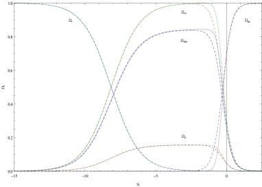
Figure 1: Background dynamics of the interacting Galileon model. We plot the evolution of the dimensionless energy densities vs $N$ where the solid lines represent the interacting Galileon model for $\alpha=-0.0075$ and the initial conditions $r_{1i}=0.0715\times 10^{-12},\>r_{2i}=7.17\times 10^{-18}.$ The dashed lines represent the energy densities in $\Lambda\textrm{CDM }$model.

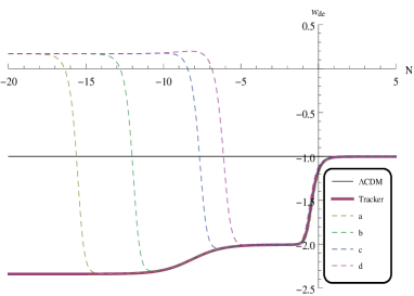
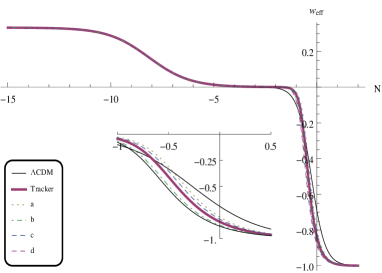
Figure 2: Evolution of $w_{de}$ and $w_{eff}$ vs $N$ for $\alpha=-0.0075$. The different curves represent several initial conditions at $N=-20$ : a) $r_{1i}=22.6\times 10^{-6},\>r_{2i}=0.52\times 10^{-38},$ b) $r_{1i}=27.1\times 10^{-10},\>r_{2i}=0.442\times 10^{-23},$ c) $r_{1i}=0.0715\times 10^{-12},\>r_{2i}=7.17\times 10^{-18}$, d) $r_{1i}=22.1\times 10^{-16},\>r_{2i}=2.7\times 10^{-2}.$ The Thick curve show the tracker solution with $r_{1}=1$, $r_{2i}=0.71\times 10^{-59}$, and the thin black line is $\Lambda\textrm{CDM }$result.

• Distance luminosity and Hubble parameter:

In this paragraph we compare the background expansion history of the interacting Galileon model with the $\Lambda$CDM using the distance modulus and the Hubble parameter. We use the Union2.1 compilation data for the Supernovae Ia type including 557 points [88] and the latest cosmic chronometer $H(z$) data used in [89] and based on the datasets in [90, 91]. The distance modulus $\mu\left(z\right)$, an observable quantity, is given in terms of the luminosity distance $d_{\textrm{L}}=\left(1+z\right)\int_{0}^{z}\frac{du}{H\left(u\right)}$ by

$$\mu\left(z\right)=5\log\left(\frac{d_{\textrm{L}}}{H_{0}\,\textrm{Mpc}}\right)+25$$ (7.1)

where $H$ is given by

$$H=H_{0}\left(\frac{r_{1}\left(0\right)}{r_{2}\left(N\right)}\right)^{5/4}\left(\frac{r_{2}\left(0\right)}{r_{2}\left(N\right)}\right)^{1/4}.$$ (7.2)

In the right panel of Fig. 3 we show examples of the evolution of the distance modulus for fixed initial conditions and coupling constant. The curves represent the scenarios including the exact solution (dot-dashed), the approximate tracking solution (dashed) and $\Lambda$CDM (solid), respectively. In the right panel we fix the coupling constant to $\alpha=-0.0075$ and vary the initial value of the radiation energy density while we keep the initial conditions on $r_{1}$ and $r_{2}$ fixed and plot the ratio between the distance modulus in our model and the distance modulus computed in the $\Lambda\textrm{CDM}$ model. As we can see the best result is reached for $\Omega_{r,i}=0.9999929.$ Exactly like the plots for the distance modulus, we see that the best ratio between the Hubble parameter in our model and the Hubble parameter in the $\Lambda\textrm{CDM}$ model with the same coupling constant and initial conditions is also reached for $\Omega_{r,i}=0.9999929.$

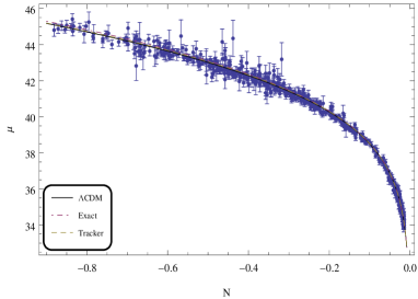
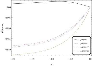
Figure 3: Left panel: Distance modulus versus $N$ for $\Omega_{ri}=0.9999929.$ Right panel: Comparison between the distance modulus in the interacting Galileon model and $\Lambda$CDM for different initial conditions on the radiation energy. In both panels we used $\alpha=-0.0075,\>r_{1i}=0.0715\times 10^{-12},\>r_{2i}=7.17\times 10^{-18},\>\Omega_{bi}=1.1013\times 10^{-6}$.

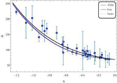
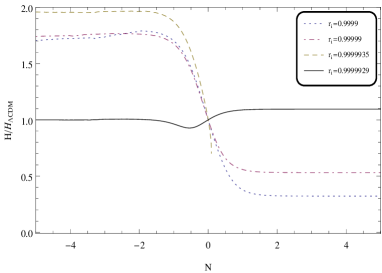
Figure 4: Left panel: Hubble parameter versus $N$ for $\Omega_{ri}=0.9999929.$ Right panel: Comparison between the Hubble parameters in the interacting Galileon model and $\Lambda$CDM. We use the same initial input values as Fig. 3.

• No-ghost and Laplacian instabilities:

In Fig. 5 we plot the evolution of $Q_{\textrm{S}}$ in different scenarios: the exact numerical solution obtained by integrating the autonomous system (4.3-4.6), the small regime solution given by Eq.(6.11), the radiation and the matter domination epochs obtained for $r_{2}$ small in the vicinity of the fixed points C and D given by Eqs.(6.19) and (6.25), respectively, and lastly the approximated tracking solution given in Eq.(6.40). As can be seen, the exact curve follows exactly the small regime solution in the radiation era (6.11), then merges at the onset of the matter domination era with the tracking solution (6.40), and the fixed points C and D solutions given by (6.19) and (6.25), respectively, before continuing alone along the tracking solution in the dS era. The evolution of the propagation speed squared of the scalar modes is plotted in Fig. 6. In the small regime, $r_{1}\ll 1$ and $r_{2}\ll 1$, the exact curve follows the estimated values of the scalar propagation speed given by (6.13) and (6.14) in the radiation and matter small regime eras, respectively. For $\alpha=-0.0075$, these values are given by $C_{\textrm{S}}^{2}\approx 0.4987$ and $C_{\textrm{S}}^{2}\approx 0.4154$ for $\Omega_{r}=1$ and $\Omega_{r}=0,$ respectively. Then, the exact curve follows the estimated values given in the eras around the points C and D given by $C_{\textrm{S}}^{2}\approx 1.667$ and $C_{\textrm{S}}^{2}\approx 1.333$ for $\Omega_{r}=1$ and $\Omega_{r}=0,$ respectively, and finally it follows the tracking solution at the onset of the matter era until the dS era. However, this behavior is highly dependent on the initial conditions. For example, in the cases (a) and (b) the exact curve enters early the tracking regime and follows the points A, C, D and ends in the dS era, while in the cases (c) and (d), the curve follows later the tracking regime and follows the points A, B, D before it ends in the dS era. This is exactly the behavior observed with $w_{\textrm{de}}.$ Finally, we can find a set of initial conditions, as shown in (e), where the scalar mode starts sub-luminal, follows the approximated tracker solution and becomes super-luminal temporarily during the eras around the fixed points C and D, before it becomes sub-luminal in the recent past until today where $C_{\textrm{S}}^{2}\left(z=0\right)\approx 0.183$. But, when it goes deeper in the dS era weak Laplacian instabilities appear since $C_{\textrm{S}}^{2}\left(z\rightarrow-1\right)\approx-0.00041$. As already noted in [46], the fact that there is a cosmological epoch where the propagation speed squared of scalar modes is greater than one does not render the model unviable because of the possibility for the absence of closed causal curves [41]. Let us finally note that even we introduced an interaction between the dark sectors the GWs propagate at the speed of light, and thus the bounds imposed simultaneously by GW170817 and GRB170807A [92, 93] are trivialy satisfied .

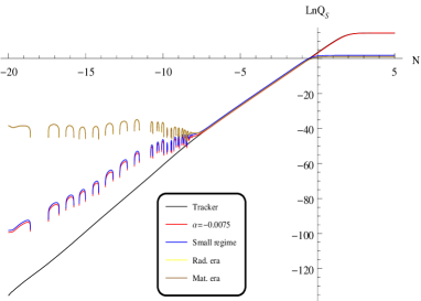
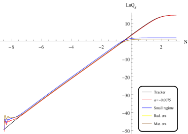
Figure 5: Left panel: Evolution of $Q_{S}$ versus $N$ in different scenarios for $\alpha=-0.0075$, $\Omega_{ri}=0.9999929,\>\Omega_{bi}=1.10125\times 10^{-6}$. For the exact calculation the initial conditions are $r_{1i}=0.0715\times 10^{-12},\>r_{2i}=7.17\times 10^{-18}$, while for the tracker we used $r_{2i}=0.71\times 10^{-59}.$ Right panel: zoom on the region $-8.5\leq N\leq 2.5$.

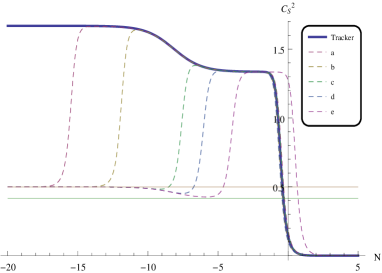
Figure 6: Evolution of $C_{\textrm{S}}^{\text{2}}$ versus $N$ for different scenarios for $\alpha=-0.0075$. The thin horizontal lines are for $C_{S}^{\text{2}}\approx 0.4987$ and $C_{S}^{2}\approx 0.4154,$ in radiation and matter dominance eras, respectively. We use the same initial input values as Fig. 2 plus the curve (e) with $r_{1i}=24.01\times 10^{-17},\>r_{2i}=7.6\times 10^{-1}$.

• Statefinder and $Om$ diagnostics

In this section, we analyze the interacting Galileon model by the statefinder diagnostic. In the $\Lambda\textrm{CDM}$ model, two fundamental geometrical probes characterize the dynamics of the universe expansion, the Hubble parameter $H$ and the deceleration parameter $q$ involving only the scale factor, its first and second derivatives with respect to time. However, with the great amount and increasing precision of the cosmological observations data and the advent of a plethora of dark energy models, the present question is how to discriminate between these models, and how to quantify the distance to the $\Lambda\textrm{CDM}$ model. Since the Hubble and deceleration parameters are no longer sensitive enough to discriminate between the different dark energy models, Sahni et al.[94] and Alam et al.[95] proposed the so-called statefinder diagnostic based on higher derivatives of the scale factor with respect to time and introduced new pair of parameters $\left\{r,s\right\}$ defined by

$$r=\frac{\dddot{a}}{aH^{3}}\quad s=\frac{r-1}{3\left(q-1/2\right)}$$

where $q=-\ddot{a}/\left(aH^{2}\right)$ is the deceleration parameter. It is expected from the design of future experiment [96, 97, 98] to obtain an estimate of these parameters. The $\Lambda\textrm{CDM}$ model corresponds to the fixed point $\left\{1,0\right\}$ in the plane $\left\{r,s\right\}.$ This feature, allows us to appreciate the behavior of models of dark energy by measuring the distance between them and the $\Lambda\textrm{CDM}$ fixed point. The full numerical analysis of the statefinder parameters is shown in Figs.(7)-(8). Fig.7 shows the time evolution of $q,$ $r$ and $s$ for different DE-DM coupling constant. In all panels the exact numerical statefinder parameters (dashed curves) are compared to the tracking solution (thick curve) and the $\Lambda\textrm{CDM}$ model results (black thin curve). Apart deviations in the recent past due to DE-DM interaction, we observe that for $\alpha=-0.0075$ the exact and the tracker curves for $q$ and $r$ are practically indistinguishable and are very close to the $\Lambda\textrm{CDM}$ curve. For the $s$ parameter and under the same setup the exact and the tracker curves merge with the $\Lambda\textrm{CDM}$ curve only in the near future and stand on in the dS era. In Fig. 8 and from left to right, we illustrate the evolution of the pairs $\left\{q,r\right\},\>\left\{q,s\right\}$ and $\left\{r,s\right\}.$ For the pairs $\left\{q,r\right\}$ and $\left\{q,s\right\}$ the exact and tracker curves for $\alpha=-0.0075$ which are indistinguishable start from the standard cold dark matter (SCDM) point where $w_{eff}=0$ and $\left\{q=1/2,\>r=1\right\}$ and converge toward the dS universe where $\left\{q=-1,\>r=1\right\}.$ In the right panel all the curves start at the dS fixed point $\left\{q=-1,\>r=1\right\},$ pass through the $\Lambda\textrm{CDM}$ fixed point $\left\{r=1,\>s=0\right\}$, and after some detours, the trajectories converge toward this point. However, for $\alpha=-0.0075$, the exact and tracking curves converge to the $\Lambda\textrm{CDM}$ fixed point without tracing visible loops. The apparition of loops is suggested from the $r$-curves, in the middle panel of Fig.7, which cross the $\Lambda\textrm{CDM}$ line from above in the recent past to below in the future (the curves with $\alpha=-0.12$ and $\alpha=-0.098,$ respectively). As can be seen, the $r$-curves which do not form loops never cross the $\Lambda\textrm{CDM}$ line. Similar conclusions can be traced from the $s$-curves in the left panel of Fig.7.

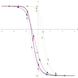
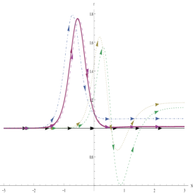
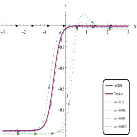
Figure 7: Evolution of the deceleration parameter $q\left(N\right),$ and the statefinder parameters $\>r\left(N\right),\>s\left(N\right)$ for different values of the coupling $\alpha$ and the with the initial conditions $r_{1i}=0.0715\times 10^{-12},\>r_{2i}=7.17\times 10^{-18},\>\Omega_{ri}=0.9999929,\>\Omega_{bi}=1.1013\times 10^{-6}.$

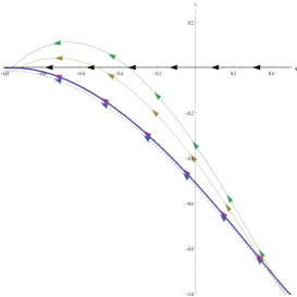
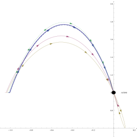
Figure 8: Statefinder diagnostic in the $r-q,\>s-q$ and $r-s$ planes for the same parameters as Fig.7.

The $Om$ diagnostic is an other very useful tool to discriminate between different cosmological models. It involves only first order derivative of the scale factor and is based on the following formula

$$Om\left(N\right)=\frac{E^{2}\left(N\right)-1}{e^{-3N}-1}$$ (7.3)

where $E\left(N\right)=H\left(N\right)/H_{0}$ is given by (7.2). We have included the radiation contribution in our analysis. For non-interacting dark energy models with constant $w_{de},$ a positive slope of $Om$ corresponds to phantom like behavior $\left(w_{de}<-1\right)$, a negative slope corresponds to quintessence like behavior $\left(w_{de}>-1\right),$ and zero slope to the cosmological constant. In Fig.(9) we show the $Om$ curves for the exact, tracker and $\Lambda$CDM calculations. For $\alpha=-0.0075$, the exact curve starts following the $\Lambda$CDM curve at the onset of the matter domination epoch, then diverge from the $\Lambda$CDM curve in the recent past until it becomes constant in the dS era. The difference in the trajectory evolution between the $\Lambda$CDM and the interacting Galileon model at the onset of DE domination epoch can be explained by the DE-DM interaction which only becomes relevant in the recent past. As we can see we have practically always a positive curvature signaling a phantom behavior.

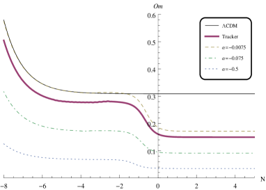
Figure 9: The $Om$ curves for different values of the coupling constant. The initial conditions are $r_{1i}=0.0715\times 10^{-12},\>r_{2i}=7.17\times 10^{-18}.$

8 Conclusion

In our present work, we considered the DE-DM interaction in the cubic Galileon model where the interaction term is proportional to Hubble parameter and Galileon dark energy in the form $Q=\alpha H\rho_{de}.$ We first assumed the existence of a dS cosmological era, which allowed us to write the free parameters in the Galileon Lagrangian in terms of the coupling constant and thus we reduced the dimension of the parameter space. Using appropriate dimensionless variables, $r_{1},\>r_{2}$ besides the radiation and baryonic energy densities, the field equations in flat FLRW background have been converted into an autonomous system of first order differential equations. The dynamical system analysis of the model has revealed the usual physical phase space reproducing the different cosmological eras, radiation domination era, matter domination era and the dark energy domination era, and possess a de Sitter expansion fate in the future.

We carried out the exact numerical integration of the dynamical systems of equations (4.14-4.17) and analyzed the evolution of the background quantities like the energy densities $\Omega_{i}$, the dark energy EoS $w_{de}$ and the total effective EoS parameters $w_{eff}$, as well as $C_{S}^{2}$ and $Q_{S}$. The conditions on the tensor modes being automatically satisfied, we derived the conditions for the avoidance of ghosts and Laplacian instabilities associated with scalar in terms of the dynamical variables and the coupling constant. The stability analysis of the critical points and the conditions for the avoidance of ghosts and Laplacian instabilities constrained the coupling constant to negative values. The existence of a stable attractor in the dS era allowed us to construct an approximated tracking solution which mimics the exact solution, particularly in the recent past before reaching the dS era. We have shown that the exact curves representing the dark energy EoS, $w_{de},$ converge to the tracker solution at early or later times depending on the initial conditions of the dynamical variables. Particularly, we obtained that along the tracker solution, $w_{de}$ follows paths belonging to the eras described by the fixed points A, C, D and E and exhibits peculiar behavior: $w_{de}=-7/3+\alpha/3$ in the radiation era, $w_{de}=-2+\alpha/3$ in the matter era, and $w_{de}=-1+\alpha/3$ in the dS era. However, depending on the initial conditions on $r_{1}$ and $r_{2}$, the exact $w_{de}$ follows one of the sequences: A, B, D, E at earlier times for $r_{1i}$ small, or A, C, D, E at later time for $r_{2i}$ small . As we can see the tracker solution is not compatible with observations since $w_{de}$ is far away from $-1$ in the matter era [47]. The same problem was met in the quintic Galileon model and solved in the framework of the extended Galileon model [45]. Then, it will be of interest to investigate the DE-DM interaction in the extended Galileon model and evaluate the combined effects of $\alpha$ and $s$ on the viability of the tracking solution.

Concerning the conditions for the avoidance of ghosts and Laplacian instabilities associated with scalar perturbations, we found that the exact curve follows exactly the small regime curve in the radiation dominated era, then merges with the tracking and the solutions around the fixed points C and D, and finally follows the tracking solution alone at in the dS era. For the evolution of the propagation speed squared of the scalar mode, we found that the mode starts super-luminal during the eras around the fixed points C and D, before it becomes sub-luminal in the recent past until entering the dS point where it takes the value $C_{\textrm{S}}^{2}\approx 4.16\times 10^{-5}$ for $\alpha=-0.0075$. In all cosmological epochs, $Q_{S}$ remains positive, while $C_{S}^{2}$ which is positive until today, $C_{\textrm{S}}^{2}\left(z=0\right)\approx 0.183,$ and in the future with $C_{\textrm{S}}^{2}\left(z\approx-0.85\right)\approx 7.35176\times 10^{-6},$ becomes weakly negative in the depth of the dS epoch where $C_{\textrm{S}}^{2}\left(z\rightarrow-1\right)\approx-0.00041$.

We have also compared the theoretical distance modulus and Hubble parameter with the observation data. We found best agreement for a set of initial conditions and coupling constant, and that for fixed initial conditions on $r_{1}$ and $r_{2}$ and $\alpha=-0.0075,$ the best agreement between the exact results of the interacting cubic Galileon model and the $\Lambda$CDM model is reached for $\Omega_{ri}=0.9999929.$

Employing the statefinder diagnostic, we found that the interacting cubic Galileon model can be distinguished from the $\Lambda$CDM model. Particularly, the parameter $s$ shows a completely different behavior starting in the matter domination era until the recent past compared to the $\Lambda$CDM model. We have also shown that all the trajectories start from the SCDM fixed point $\left\{q=1/2,\>r=1\right\}$ but do not converge all to the dS fixed point $\left\{q=-1,\>r=1\right\}$ due to their phantom evolution. However for $\alpha=-0.0075$, the evolution of exact and the tracking curves are indistinguishable and the approach to the dS point becomes more precise. In the $r-s$ plane, all the trajectories start approximatively at the point $\left\{s=-1,\>r=1\right\}$, pass through the $\Lambda$CDM fixed point, and depending on the value of the coupling constant and the initial conditions, trace loops before converging to the $\Lambda$CDM point. In addition we used the $Om$ diagnostic, where we showed that the exact and tracking curves are indistinguishable and begin to diverge from the $\Lambda$CDM model at the onset of the late time acceleration era.

In summary, we have shown that the interacting Cubic Galileon model constitute a viable dark energy model for a DE-DM interaction function in the form $Q=\alpha H\rho_{de}$, since it is not plagued by a negative evolution of dark matter density in the dS era, unlike the case of constant $w_{\textrm{de}}$. However, it suffers from the appearance of soft Laplacian instabilities in the far future of the dS era. A full treatment of the evolution of matter density perturbations and gravitational potentials and a joint data analysis using observational data such Supernovae type Ia, BAO distance measurements, Weak gravitational lensing, and CMB observations are necessary to place constraints on the coupling constant for the exact and the approximated tracker solutions. We leave these issues for forcoming works.

References

- [1] A. G. Riess et al. Astron. J. 116, 1009 (1998) [arXiv.9805201[astro-ph]].
- [2] A. G. Riess et al. Astron. J. 117, 707 (1999) [arXiv.9810091 [astro-ph]].
- [3] S. Perlmutter et al. Astrophys. J. 515, 565 (1999) [arXiv:9812133 [astro-ph]].
- [4] D. N. Spergel et al. [WMAP Collaboration], Astrophys. J. Suppl. 148, 175 (2003) [arXiv:0302209 [astro-ph]].
- [5] D. J. Eisenstein et al. [SDSS Collaboration], Astrophys. J. 633, 560 (2005) [arXiv:05001171 [astro-ph]].
- [6] P. Astier et al. Astron. Astrophys. 447, 31 (2006) [arXiv:05100447 [astro-ph]].
- [7] P. A. R. Ade et al. [Planck Collaboration], Astron. Astro- phys. 594 , A13 (2016) [arXiv:1502.01589 [astro-ph.CO]].
- [8] E. J. Copeland, M. Sami and S. Tsujikawa, Int. J. Mod. Phys. D 15, 1753 (2006) [arXiv:0603057 [hep-th]].
- [9] E.V. Linder, Rep. Prog. Phys. 71, 056901 (2008) [arXiV.0801.2968 [astro-ph]].
- [10] A. Silvestri and M. Trodden, Rep. Prog. Phys. 72, 096901 (2009) [arXiv.094.0024] [astrp-ph.CO]].
- [11] V. Sahni and A. A. Starobinsky, Int. J. Mod. Phys. D 9, 373 (2009) [arXiv.9904398 [astro-ph]].
- [12] P. J. Steinhardt, in Critical Problems in Physics, edit by V. L. Fitch and D. R. Marlow (Princeton University Press, Princeton, NJ, 1997).
- [13] S. Weinberg, Rev. Mod. Phys. 61, 1 (1988).
- [14] Y. Fujii, Phys. Rev. D 26, 2580 (1982).
- [15] L. H. Ford, Phy. Rev. D 35, 2339 (1987).
- [16] C. Wetterich, Nucl. Phys. B 302, 668 (1988).
- [17] B. Ratra and J. Peebles, Phys. Rev. D 37, 321 (1988).
- [18] Y. Fujii and T. Nishioka, Phys. Rev. D 42, 361 (1990)
- [19] R. R. Caldwell, R. Dave and P. J. Steinhardt, Phys. Rev. Lett. 80, 1580 (1998) [arXiv:9708069 [astro-ph]].
- [20] C. Armendariz-Picon, V. Mukhanov, and P. J. Steinhardt, Phys. Rev. Lett. 85, 4438 (2000) [arXiv:0004134 [hep-th]].
- [21] A. Sen, JHEP 0204, 048 (2002) [arXiv:0203211 [astro-ph]].
- [22] A. Sen, JHEP 0207, 065 (2002) [arXiv:0203265 [hep-th]].
- [23] A. Yu. Kamenshchik, U. Moshella and V. Pasquier, Phys. Lett. B 511, 265 (2001) [ArXiv:0103004 [gr-qc]].
- [24] N. Bilic, G. B. Tupper and R. D. Viollier, Phys. Lett. B 535, 17 (2002) [ArXiv:0111325 [astro-ph]].
- [25] G. R. Dvali, G. Gabadadze and M. Porrati, Phys. Lett. B 485, 208 (2000) [arXiv:0005016 [hep-th]].
- [26] A. Nicolis, R. Rattazzi and E. Trincherini, Phys. Rev. D 79, 064036 (2009) [arXiv:0811.2197 [hep-th]].
- [27] D. Gorbunov, K. Koyama and S. Sibiryakov, Phys. Rev. D 73, 044016 (2006) [arXiv:0512097 [hep-th]].
- [28] K. Koyama and R. Maartens, JCAP 0601, 016 (2006) [arXiv:0511634 [astro-ph]].
- [29] I. Sawicki and S. M. Carroll, [arXiv:0510364 [astro]].
- [30] M. Fairbairn and A. Goobar, Phys. Lett. B 642 , 432 (2006) [arXiv:0511029 [astro-ph]].
- [31] R. Maartens and E. Majerotto, Phys. Rev. D 74, 023004 (2006) (arXiv:0603353 [astro-ph]].
- [32] U. Alam and V. Sahni, Phys. Rev. D 73, 084024 (2006) [arXiv:0511473 [astro-ph]].
- [33] Y. S. Song, I. Sawicki and W. Hu, Phys. Rev. D 75, 064003 (2007) [arXiv:0606286 [astro-ph]].
- [34] M. A. Luty, M. Porrati and R. Rattazzi, JHEP 0309, 029 (2003) [arXiv:0303116][hep-th]].
- [35] A. Nicolis and R. Rattazzi, JHEP 0406, 059 (2004) [arXiv:0404159][hep-th]].
- [36] C. Deffayet, G. Esposito-Farese and A. Vikman, Phys. Rev. D 79, 084003 (2009) [arXiv:0901.1314].
- [37] C. Deffayet, S. Deser and G. Esposito-Farese, Phys. Rev. D 80, 064015 (2009) [arXiv:0906.1957].
- [38] N. Chow and J. Khoury, Phys. Rev. D 80, 024037 (2009) [arXiv:0605.1225[hep-th]].
- [39] T. Kobayashi, Phys. Rev. D 81, 103533 (2010) [arXiv:1003.3281 [arXiv:09124538 [astro-ph.CO]].
- [40] T. Kobayashi, H. Tashiro and D. Suzuki, Phys. Rev. D 81, 063513 (2010) [arXiv:0912.4641 [astro-ph.CO]].
- [41] R. Gannoudji and M. Sami, Phys. Rev D 82, 024011 (2010) [arXiv:1004.2808 [gr-qc]].
- [42] A. Ali, R. Gannoudji and M. Sami, Phys. Rev D 82, 103015 (2010) [arXiv:1008.1588 [astro-ph.CO]].
- [43] D. F. Mota, M. Sandstad and T. Zlosnik, JHEP 1012, 051 (2010) [arXiv.1009.6151 [astro-ph.CO]].
- [44] A. de Felice, S. Mukhoyama and S. Tsujikawa, Phys. Rev. D 82, 023524 (2010) [arXiv: 1006.0281] [astro-ph.CO]].
- [45] A. De Felice, S. Tsujikawa, JCAP 1202: 007, (2012) [arXiV:1110.3878 [gr-qc]].
- [46] A. De Felice, S. Tsujikawa, Phys. Rev. Lett. 105, 111301 (2010) [arXiV:1007.2700 [astro-ph.CO]].
- [47] S. Nesseris, A. De Felice, S. Tsujikawa, Phys. Rev. D 82, 124054, (2010) [arXiv:1010.0407]
- [48] S. Capozziello, Int. J. Mod. Phys. D 11, 483, (2002) [arXiv:020103 [gr-qc]].
- [49] S. Capozziello, V. F. Cardone, S. Carloni and A. Troisi, Int. J. Mod. Phys. D 12, 1969 (2003) [arXiv:0307018 [astro-ph]].
- [50] S. M. Carroll, V. Duvvuri, M. Trodden and M. S. Turner, Phys. Rev. D 70, 043528 (2004) [arXiv:0306438 [astro-ph]].
- [51] S. Nojiri and S. D. Odintsov, Phys. Rev. D 68, 123512 (2003) [arXiv:0307288 [hep-th]].
- [52] L. Amendola, Phys. Rev. D 60, 043501 (1999) [arXiv:9904120 [astro-ph]].
- [53] J. P. Uzan, Phys. Rev. D 59, 123510 (1999).
- [54] T. Chiba, Phys. Rev. D 60, 083508 (1999) [arXiv:9903094 [gr-qc]].
- [55] N. Bartolo and M. Pietroni, Phys. Rev. D 61, 023518 (2000) [arXiv:9908521 [hep-ph]].
- [56] F. Perrotta, C. Baccigalupi and S. Matarrese, Phys. Rev. D 61, 023507 (2000) [arXiv:9906066 [astro-ph]].
- [57] A. Riazuelo and J. P. Uzan, Phys. Rev. D 66, 023525 (2002) [arXiv:0107386 [astro-ph]]..
- [58] S. Nojiri, S. D. Odintsov and M. Sasaki, Phys. Rev. D 71, 123509 (2005) [arXiv:0504052 [hep-th]].
- [59] S. Nojiri and S. D. Odintsov, Phys. Lett. B 631, 1 (2005) [arXiv:0604431 [astro-ph]].
- [60] C. Wetterich, Nucl. Phys. B 302, 668 (1988).
- [61] C. Wetterich, Astron. Astrophys. 301, 321 (1995) [arXiv:940825 [hep-th]].
- [62] D. Tocchini-Valentini and L. Amendola, Phys. Rev. D 65, 063508 (2002) [astro-ph/0108143];
- [63] R. G. Cai and A. Wang, JCAP 0503, 002 (2005) [hep- th/0411025];
- [64] X. Zhang, Mod. Phys. Lett. A 20, 2575 (2005) [astro-ph/0503072];
- [65] M. S. Berger and H. Shojaei, Phys. Rev. D 73, 083528 (2006) [gr-qc/0601086];
- [66] B. Hu and Y. Ling, “Interacting dark energy, Phys. Rev. D 73, 123510 (2006) [hep-th/0601093];
- [67] H. M. Sadjadi and M. Alimohammadi, Phys. Rev. D 74, 103007 (2006) [gr-qc/0610080].
- [68] L. P. Chimento, A. S. Jakubi, D. Pav n and W. Zimdahl, Phys. Rev. D 67, 083513 (2003) [astro- ph/0303145];
- [69] P. C. Ferreira, D. Pav n and J. C. Carvalho, Phys. Rev. D 88, 083503 (2013) [arXiv:1310.2160 [gr-qc]].
- [70] S. del Campo, R. Herrera and D. Pav n, Phys. Rev. D 78, 021302 (2008) [arXiv:0806.2116 [astro-ph]]; JCAP 0901, 020 (2009) [arXiv:0812.2210 [gr-qc]]; Phys. Rev. D 91, no. 12, 123539 (2015) [arXiv:1507.00187 [gr-qc]].
- [71] B. Wang, Y. G. Gong and E. Abdalla, Phys. Lett. B 624, 141 (2005) [hep-th/0506069].
- [72] Y. Zhang, T. Y. Xia and W. Zhao, Class. Quant. Grav. 24, 3309 (2007) [gr-qc/0609115];
- [73] W. Zhao, Int. J. Mod. Phys. D 18, 1331 (2009) [arXiv:0810.5506 [gr-qc]].
- [74] J. H. He, B. Wang and E. Abdalla, Phys. Rev. D 83, 063515 (2011) [arXiv:1012.3904 [astro-ph.CO]].
- [75] A. A. Costa, X. D. Xu, B. Wang, E. G. M. Ferreira and E. Abdalla, Phys. Rev. D 89, no. 10, 103531 (2014) [arXiv:1311.7380 [astro- ph.CO]].
- [76] B. Wang, E. Abdalla, F. Atrio-Barandela and D. Pav n, Rept. Prog. Phys. 79, no. 9, 096901 (2016) [arXiv:1603.08299 [astro-ph.CO]].
- [77] L. Amendola, Phys. Rev. D 60, 043501 (1999) [arXiv:9904120 [astro-ph]].
- [78] L. Amendola, Phys. Rev. D 62, 043511 (2000) [arXiv:9908023 [astro-ph]].
- [79] L. Santos, W. Zaho, E. G. M. Ferreira and J. Quintin, Phys. Rev. D 96, 103529 (2017) [arXiv:0707.06827 [astro-ph.CO]].
- [80] E. Di Valentino, A. Melchiorri and O. Mena, Phys. Rev. D 96, 043503 (2017) [arXiv:1704.08342v1 [astro-ph.CO]]
- [81] N. Aghanim et al. [Planck Collaboration], Astron. Astrophys. 596, A107 (2016) [arXiv:1605.02985 [astro-ph.CO]].
- [82] A. G. Riess et al, Astrophys. J. 826, no.1, 56 (2016) [arXiv:1604.01424 [astro-ph.CO]].
- [83] H. Kodama and M. Sasaki, Prog. Theor. Phys. Suppl. Vol. 78, 1 (1984).
- [84] O. Bertolami, F. Gil Pedro, and M. Le Delliou. Phys. Lett. B 654, 165 (2007) [arXiv:0703462 [astro-ph]].
- [85] M. Baldi. Mon. Not. R. Astron. Soc. 414, 116 (2011) [arXiv:1012.0002 [astro-ph.CO]].
- [86] P. A. R. Ade et al. [Planck Collaboration], “Planck 2015 results. XIII. Cosmological parameters”, Astron. Astrophys. 594, A13 (2016) [ArXiv:1502.01586 [astro-ph[CO]].
- [87] C. G. Boehmer, G. Caldera-Cabral, R. Lazkoz and R. Maartens, Phys. Rev. D 78, 023505 (2008) [arXiv:0801.1565 [gr-qc]].
- [88] N. Suzuki, D. Rubin, C. Lidman, G. Aldering, R. Amanullah, K. Barbary, L. F. Barrientos and J. Botyanszki et al. Astrophys. J. 746, 85 (2012) [arXiv:1105.3470 [astro-ph.CO]].
- [89] S. Basilakos and S. Nesseris, Phys. Rev. D 96, 063517 (2017) [arXiv:1705.08797 [astro-ph.CO]
- [90] M. Moresco, L. Pozzetti, A. Cimatti, R. Jimenez, C. Maraston, L. Verde, D. Thomas, A. Citro, R. Tojeiro and D. Wilkinson, JCAP 1605, 014 (2016) [arXiv:1604.00183 [astro-ph.CO]]
- [91] C. Zhang, H. Zhang, S. Yuan, T.-J. Zhang and Y.-C. Sun, Res. Astron. Astrophys. 14, 1221 (2014) [arXiv:1207.4541 [astro-ph.CO]].
- [92] B. P. Abbott et al. [LIGO Scientific and Virgo Collaborations], Phys. Rev. Lett. 119, no.16, 141101 (2017) [arXiv:1709.09660 [gr-qc]].
- [93] B. P. Abbott et al. [LIGO Scientific and Virgo and Fermi-GBM and INTEGRAL Collaborations], The Astrophysical Journal Letters. 848, L13 (2017) [arXiv:1710.05834 [astro-ph]].
- [94] V. Sahni, T. D. Saini, A. A. Starobinsky and U. Alam, JETP Lett. 77, 201 (2003) [Pisma Zh. Eksp. Teor. Fiz. 77, 249 (2003)] [arXiv:0201498 [astro-ph]].
- [95] U. Alam, V. Sahni, T. D. Saini and A. A. Starobinsky, Mon. Not. Roy. Astron. Soc. 344, 1057 (2003) [arXiv:0303009 [astro-ph]].
- [96] J. Albert et al. [SNAP collaboration][astro-ph/0507458].
- [97] J. Albert et al.[SNAP collaboration][astro-ph/0507459].
- [98] Eric. V. Linder, [SNAP collaboration] [astro-ph/0406186 ].