Characterising the nonequilibrium stationary states of Ornstein-Uhlenbeck processes
Abstract
We characterise the nonequilibrium stationary state of a generic multivariate Ornstein-Uhlenbeck process involving degrees of freedom. The irreversibility of the process is encoded in the antisymmetric part of the Onsager matrix. The linearity of the Langevin equations allows us to derive closed-form expressions in terms of the latter matrix for many quantities of interest, in particular the entropy production rate and the fluctuation-dissipation ratio matrix. This general setting is then illustrated by two classes of systems. First, we consider the one-dimensional ferromagnetic Gaussian spin model endowed with a stochastic dynamics where spatial asymmetry results in irreversibility. The stationary state on a ring is independent of the asymmetry parameter, whereas it depends continuously on the latter on an open chain. Much attention is also paid to finite-size effects, especially near the critical point. Second, we consider arrays of resistively coupled electrical circuits. The entropy production rate is evaluated in the regime where the local temperatures of the resistors have small fluctuations. For networks the entropy production rate grows linearly with the size of the array. For networks a quadratic growth law violating extensivity is predicted.
1 Introduction
The everlasting interest for nonequilibrium phenomena in Statistical Physics has experienced a considerable upsurge in the last decades with the emergence of a series of general results known as fluctuation theorems. These theoretical developments have emphasised the central role of the rate of entropy production per unit time, which is the key quantity involved in the Gallavotti-Cohen fluctuation theorem [1] (see also [2, 3, 4, 5, 6, 7]). Even though the entropy production rate appears as a fundamental quantity characterising nonequilibrium stationary states, the latter possess many other features of interest, including a violation of the fluctuation-dissipation theorem characteristic of equilibrium states in the linear-response regime and non-local fluctuations in the large-deviation regime [8, 9, 10, 11].
The goal of this work is to investigate the most salient characteristic features of nonequilibrium stationary states within a unified framework in a specific class of models which lend themselves to an analytic approach, namely linear Langevin systems. These systems can be viewed as higher-dimensional extensions of the well-known Ornstein-Uhlenbeck process [12], describing the velocity of a Brownian particle in one dimension,
| (1.1) |
where is the friction coefficient and is a Gaussian white noise with amplitude , i.e.,
| (1.2) |
The system equilibrates under the combined effects of linear damping and noise. The equilibrium probability distribution of the velocity is the Maxwell-Boltzmann distribution, i.e., a Gaussian law with variance . The Ornstein-Uhlenbeck process is reversible and obeys detailed balance with respect to the above distribution. The Einstein relation is an example of an equilibrium fluctuation-dissipation relation.
Generalising the Ornstein-Uhlenbeck process to several linearly coupled degrees of freedom appears as a very natural construction. The first occurrence of a multivariate Ornstein-Uhlenbeck process can be traced back to [13]. Such a process is defined by linear Langevin equations describing the evolution of coupled dynamical variables. Remarkably enough, in stark contrast with the historical case recalled above, a generic multivariate Ornstein-Uhlenbeck process is irreversible [14, 15, 16, 17, 18]. To close this introduction of the problem, let us mention related works concerning the structure of either dissipative or otherwise irreversible dynamical systems near fixed points, where the dynamical equations can be linearised [19, 20, 21, 22]. In the stochastic setting, this line of thought leads to consider multivariate Ornstein-Uhlenbeck processes.
This paper is devoted to a systematic characterisation of the nonequilibrium stationary states of multivariate Ornstein-Uhlenbeck processes. The linearity of the Langevin equations governing these processes allows us to use tools from linear algebra. In section 2, devoted to the general framework, we demonstrate that the amount of irreversibility is measured by the antisymmetric part of the Onsager matrix . Multivariate Ornstein-Uhlenbeck processes are defined in section 2.1, the Sylvester equation governing their steady state is derived in section 2.2, and their irreversibility is characterised in section 2.3. The various quantities characterising their nonequilibrium stationary state are then derived in terms of the matrix or of its associated Hermitian form : stationary probability current (section 2.4), entropy production rate (section 2.5), correlation, response and fluctuation-dissipation ratio (section 2.6). Various other facets of the problem are also investigated, in particular the effect of a linear change of coordinates (section 2.7), a formal investigation of the case where the friction matrix (see (2.2)) is diagonalisable (section 2.8), cyclically symmetric processes (section 2.9) and the case of two degrees of freedom (section 2.10).
We then analyse in detail two different examples of physical systems giving rise to multivariate Ornstein-Uhlenbeck processes. Our first example (sections 3 and 4) is borrowed from the microscopic world of kinetic spin systems. We consider the one-dimensional ferromagnetic Gaussian spin model endowed with a stochastic dynamics where spatial asymmetry results in irreversibility, along the lines of earlier studies on the Ising and spherical ferromagnets [23, 24, 25, 26, 27, 28, 29, 30, 31, 32, 33, 34]. The geometry of a finite ring is discussed in section 3. In this situation, the asymmetric dynamics corresponds to a cyclically symmetric process, and the stationary state is independent of the asymmetry parameter . We successively investigate the statics of the model (section 3.1), the conventional gradient dynamics (section 3.2), the asymmetric dynamics (section 3.3), and the key observables characterising the resulting nonequilibrium stationary state, first in the thermodynamic limit (section 3.4) and then on finite-size systems (section 3.5). Section 4 is devoted to the model on a finite open chain. There, at variance with the ring geometry, the stationary state depends continuously on the asymmetry parameter . We study the statics of the model (section 4.1), general properties of the asymmetric dynamics (section 4.2), the spectrum of the friction matrix (section 4.3), the first few system sizes (section 4.4), and the main features of the nonequilibrium stationary state (section 4.5). We then turn to more detailed investigations of the model, both in the small- regime (section 4.6) and in the totally asymmetric case (section 4.7). Our second class of examples of multivariate Ornstein-Uhlenbeck processes originates in macroscopic physics. We consider arrays of resistively coupled electrical circuits, where resistors are sources of thermal noise. Within this setting, irreversibility is brought about by an inhomogeneous temperature profile. The main emphasis is on the entropy production rate per unit time in the regime where the fluctuations of the temperature profile are small. We successively consider networks (section 5.1) and networks (section 5.2). The scaling of the entropy production rate with the network size is very different in both cases. Section 6 contains a brief discussion of our findings. Two appendices contain the derivations of the entropy production amplitude on the open spin chain (A) and of the amplitude matrices giving the entropy production rates on both types of electrical arrays (B).
2 General framework
2.1 The model
A multivariate Ornstein-Uhlenbeck process [13, 14, 15] (see also [35], and [16, 17, 18] for reviews) is a diffusion process defined by coupled linear Langevin equations of the form
| (2.1) |
(), i.e., in vector and matrix notations,
| (2.2) |
The are Gaussian white noises such that
| (2.3) |
i.e.,
| (2.4) |
Throughout this work boldface symbols denote vectors and matrices, and the superscript denotes the transpose of a vector or of a matrix.
The process under study is thus defined by two real matrices of size : the noise covariance matrix or diffusion matrix , which is symmetric by construction, and the friction matrix , which is not symmetric in general. In what follows, we assume that is a positive definite matrix, and that is the opposite of a stability (or Hurwitz) matrix. This means that all its eigenvalues , which are in general complex, obey
| (2.5) |
We introduce for further reference the spectral gap
| (2.6) |
The above assumptions exclude degenerate cases. They ensure that the process relaxes exponentially fast to in the absence of noise, and to a fluctuating stationary state with Gaussian statistics in the presence of noise. The main goal of this work is to characterise various features of the latter state, which is generically a nonequilibrium stationary state.
2.2 Relaxation and stationary state
The relaxation of the process from its (deterministic) initial value is encoded in the Green’s function
| (2.7) |
which obeys
| (2.8) |
with . The hypothesis made on the friction matrix ensures that falls off exponentially fast to zero. We have
| (2.9) |
The process is Gaussian, as it can be expressed linearly in terms of the Gaussian white noises . Its statistics at any given time is entirely characterised by its mean value, , and by its full equal-time correlation matrix
| (2.10) |
Equation (2.9) implies
| (2.11) |
It can be checked that obeys the differential equation
| (2.12) |
The stationary state of the process is therefore Gaussian, with zero mean, and characterised by the stationary covariance matrix
| (2.13) |
This stationary state is therefore characterised by the probability density
| (2.14) |
Equation (2.12) implies
| (2.15) |
This is the key equation of the problem, relating the stationary covariance matrix to the friction and diffusion matrices and defining the process. Linear matrix equations of this type are referred to as Sylvester (or Lyapunov) equations.
2.3 Reversible vs. irreversible processes
The condition for the process (2.1) to be reversible, known for long [14, 16, 17, 18], is that the matrix product be symmetric, i.e.,
| (2.16) |
In this situation, each term in the left-hand side of (2.15) is separately equal to . The stationary covariance matrix reads
| (2.17) |
The corresponding stationary state is an equilibrium state.
Whenever the symmetry condition (2.16) is not obeyed, the process is irreversible, with a nonequilibrium stationary state. Solving the Sylvester equation (2.15) for the covariance matrix is more difficult than inverting the friction matrix . We parametrise the matrices , and by setting
| (2.18) |
The matrix is the Onsager matrix of kinetic coefficients [2, 18]. Its antisymmetric part provides a measure of the amount of irreversibility of the process. If the process is reversible, is symmetric and vanishes.
It is advantageous to recast the matrix in the following balanced form:
| (2.19) |
where is the imaginary unit, whereas , the positive square root of the diffusion matrix , is a symmetric positive definite matrix. The matrix thus defined is both dimensionless and Hermitian. Its entries are purely imaginary, and so is a real antisymmetric matrix. As a consequence, the eigenvalues of occur in pairs of opposite real numbers (unless ). Its spectral radius, i.e., its largest positive eigenvalue,
| (2.20) |
2.4 Stationary probability current
In the stationary state, following the Fokker-Planck approach [16, 17, 18], the probability current reads
| (2.21) |
where the stationary probability density is given by (2.14). We thus obtain
| (2.22) |
i.e.,
| (2.23) |
where the mobility tensor reads (see (2.18))
| (2.24) |
The stationary probability current is therefore proportional to , the matrix measuring the irreversibility of the process.
2.5 Entropy production rate
Associating an increase of entropy to an irreversible process is one of the possible statements of the second law of Thermodynamics. In more recent times, much attention has been devoted to the rate of entropy production per unit time for an open system [38, 39]. The latter rate is also the key quantity involved in the Gallavotti-Cohen fluctuation theorem [1]. By now, it is commonly recognised as being a fundamental quantity characterising a nonequilibrium stationary state.
In the present context of diffusion processes, a general expression for the entropy production rate per unit time in the stationary state seemingly appears for the first time in print in [40] (see also [22, 41, 42, 43, 44] and [45, 46]). In our notations, this reads
| (2.25) |
where the average is taken over the stationary state measure of the process. As a consequence of (2.18) and (2.24), we have , hence
| (2.26) |
Using (2.23) and (2.24), the rightmost expression can be recast into the more familiar form [47]
| (2.27) |
As expected, is strictly positive if the process is irreversible, and it vanishes only if the process is reversible. Furthermore, since the stationary state is Gaussian with covariance matrix , we have , and so
| (2.28) | |||||
These formulas express the entropy production rate as a quadratic form in the matrices , and characterising the irreversibility of the process. Finally, using again (2.18), (2.28) can be recast into the following expressions
| (2.29) |
involving neither the covariance matrix nor its inverse explicitly.
2.6 Correlation, response and fluctuation-dissipation ratio
We now turn to an investigation of the dynamics of the process, both in its transient regime and in its stationary state. Keeping in line with recent studies of slow dynamics and aging phenomena (see [48, 49, 50] for reviews), we focus our attention onto the correlation, response and fluctuation-dissipation ratio.
The correlation matrix is defined as
| (2.30) |
where the two times and are such that . This quantity obeys
| (2.31) |
with initial value for , hence (see (2.7))
| (2.32) |
The response matrix is defined as
| (2.33) |
where the ordering fields are linearly coupled to the dynamical variables , i.e., they are added to the noises on the right-hand side of (2.1). We thus readily obtain
| (2.34) |
In the stationary state, keeping the time lag fixed, the stationary correlation and response matrices read
| (2.35) |
We have therefore
| (2.36) |
The latter formula can be reshaped by introducing a dimensionless stationary fluctuation-dissipation ratio (FDR) matrix , such that
| (2.37) |
This definition agrees with the usage in the literature on slow dynamics and aging phenomena [50, 51]. The diffusion matrix plays the role of temperature. The fact that and occur in the rightmost positions on both sides of (2.37) is due to the conventions used in the definitions (2.30), (2.33) of the correlation and response matrices. We thus obtain
| (2.38) |
Using (2.18) and (2.19) yields
| (2.39) |
In the case of a reversible process (), we have and the equilibrium fluctuation-dissipation theorem is recovered as
| (2.40) |
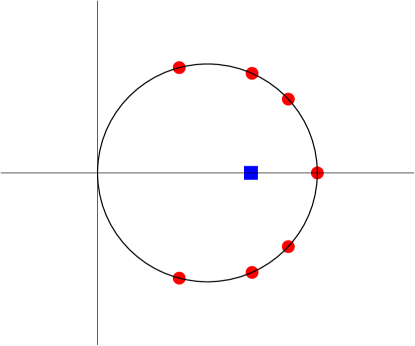
In the general situation of an irreversible process, the FDR matrix is non-trivial. The second expression of (2.39) shows that its eigenvalues are of the form
| (2.41) |
where are the eigenvalues of , introduced below (2.19). The therefore lie on the circle with diameter [0,1] in the complex plane, and they occur in complex conjugate pairs (unless ). The center of mass of these eigenvalues defines the typical FDR
| (2.42) |
This quantity is real and such that , the upper bound being attained for reversible processes. Figure 1 shows a sketch of the spectrum of the FDR matrix in a typical situation with .
2.7 Considerations on reparametrisation
In this section we investigate the effect of a reparametrisation, i.e., of a change of coordinates. In order to keep the linearity of the process (2.1), we restrict ourselves to a linear change of coordinates of the form
| (2.43) |
where is an invertible matrix.
In terms of the new coordinates , the process is transformed into a similar one, characterised by the new matrices
| (2.44) |
The matrices and transform as , i.e.,
| (2.45) |
whereas the matrices and transform as
| (2.46) |
and
| (2.47) |
The matrices , and are respectively conjugate to , and , so that their spectra are invariant under reparametrisation. The entropy production rate , the typical FDR and the asymmetry index are also invariant under reparametrisation. This corroborates the intrinsic nature of these quantities.
It is worth investigating to what extent the process (2.1) can be simplified by means of a suitably chosen linear reparametrisation. Not much can be gained on the side of the friction matrix, as and have the same spectrum. This invariance could be expected as well, as the spectrum of encodes the relaxation times of the process. The diffusion matrix can however, at least in principle, always be brought to the canonical form
| (2.48) |
corresponding to independent normalised white noises, by choosing .
2.8 The case where the friction matrix is diagonalisable
As already stated, solving the Sylvester equation (2.15) for the covariance matrix is more difficult than inverting the friction matrix . The generic situation where is diagonalisable can however be formally dealt with as follows [16]. Assume that has a biorthogonal system of left and right eigenvectors such that and , in Dirac notation, with
| (2.49) |
We have then
| (2.50) |
Equation (2.11) implies
| (2.51) | |||||
In particular, the stationary covariance matrix reads
| (2.52) |
After reduction the denominator of this expression reads
| (2.53) |
The first factor, equal to , has degree in the entries of , whereas the second factor has degree . Altogether, is a polynomial of degree . This degree equals the number of independent entries in the symmetric matrix .
With the same conventions, we have
| (2.54) |
When the process is reversible, i.e., if (2.16) holds, it can be checked that the matrix element vanishes whenever and are different, and so vanishes, as should be.
This scheme will be used several times in the course of this work, starting with section 2.9. In the happy instances where either and commute or is simple enough, quantities of physical interest such as can also be expressed in terms of the eigenvectors of .
2.9 Cyclic symmetry
As usual, the complexity of the problem can be reduced in the presence of symmetries. In this section we consider cyclically symmetric processes, where the dynamical variables live on the sites labelled of a ring of points and the dynamics is invariant under discrete translations along the ring. The matrices and are therefore circulant matrices, whose entries and only depend on the difference mod . For instance, for this reads
| (2.55) |
The property that is symmetric imposes .
In this setting, it is natural to use the discrete Fourier transform
| (2.56) |
We recall that the indices and are understood mod . If needed, they can therefore be restricted to the range . Cyclic symmetry brings out a considerable simplification. All matrices pertaining to the problem are diagonal in the Fourier basis, and therefore commute with each other. The eigenvalues of a cyclically symmetric matrix indeed coincide with its discrete Fourier amplitudes .
The diffusion matrix is symmetric, i.e., we have , and so is real. The friction matrix is not symmetric in general, and so is complex, and is its complex conjugate, so that
| (2.57) |
In this context, the process is reversible if and only is symmetric, i.e., is real. The Sylvester equation (2.15) yields
| (2.58) |
We have thus
| (2.59) | |||||
| (2.60) | |||||
| (2.61) | |||||
| (2.62) |
and finally
| (2.63) |
Let us add a remark on finite-ranged matrices. Let be a circulant matrix such that for only. The integer is dubbed the range of the matrix . As soon as the system size obeys , the amplitudes labelled by the discrete Fourier index are the restriction to the quantised momenta
| (2.64) |
of the trigonometric polynomial
| (2.65) |
which is independent of . When is symmetric, the above condition on the system size can be relaxed to . We shall see an example of such a situation with in section 3, devoted to the Gaussian spin model on a ring.
2.10 The case
To close this general section, we give explicit expressions of all quantities introduced so far in the case of two coupled degrees of freedom. This situation already exhibits most of the generic features of multivariate Ornstein-Uhlenbeck processes (see [52] for a recent account).
We parametrise the friction and diffusion matrices as
| (2.66) |
The friction matrix has positive eigenvalues for and , whereas the diffusion matrix is positive definite for and .
The reversibility condition (2.16) amounts to one single bilinear condition:
| (2.67) |
The solution of the Sylvester equation (2.15) reads
| (2.68) | |||||
Let us introduce the irreversibility parameter (see (2.67))
| (2.69) |
Equation (2.18) yields
| (2.70) |
The entropy production rate reads
| (2.71) |
Equation (2.39) yields
| (2.72) |
and
| (2.73) |
We have therefore
| (2.74) |
and
| (2.75) |
In the present situation, there is one single reversibility condition (2.67), and therefore one single irreversibility parameter . As a consequence, all the quantities characterising the irreversibility are related to each other. We have indeed
| (2.76) |
3 The Gaussian spin model on a ring
Our first example of a multivariate Ornstein-Uhlenbeck process originates in a microscopic model, which is the one-dimensional version of the ferromagnetic Gaussian spin model [53]. We shall endow the model with a dynamics where spatial asymmetry results in irreversibility. The main control parameters will be the system size and the asymmetry parameter . In this section we investigate the dynamics on a ring, whereas the more intricate situation of an open chain will be dealt with in section 4.
3.1 Statics
Let us begin with a brief report on the statics of the model. We consider the geometry of a finite ring of sites (), with periodic boundary conditions. Each site hosts a continuous spin . Throughout section 3, the index is understood mod . At infinite temperature, each spin has a Gaussian distribution such that . The weight of a spin configuration is therefore proportional to , where the free action reads
| (3.1) |
Interactions between spins are described by the nearest-neighbor ferromagnetic Hamiltonian
| (3.2) |
with . At temperature , the weight of a spin configuration is therefore proportional to , where the full action reads
| (3.3) |
with
| (3.4) |
The model owes its name to the fact that its Boltzmann weight is Gaussian. Its statics is characterised by the covariance matrix whose entries are . By definition, is the inverse of the symmetric matrix associated with the quadratic form (3.3). The non-zero elements of are and , with periodic boundary conditions. Translational invariance allows one to use the discrete Fourier transform introduced in section 2.9. As anticipated there, all the quantities labelled by the Fourier index are the restrictions of smooth functions of to the discrete set of momenta
| (3.5) |
In Fourier space, with the same conventions as in section 2.9, we have
| (3.6) |
and therefore , with
| (3.7) |
The range of is , and so the above expression holds for all .
The model is well-defined as long as the quadratic form (3.3) is positive definite. This condition amounts to requesting that all the eigenvalues , which appear as denominators in (3.7), are positive. The smallest of them, corresponding to , i.e., , reads . It vanishes at the critical point
| (3.8) |
The model therefore exists only in its high-temperature phase (). The existence of a non-zero critical temperature in one dimension underlines the lack of realism of the ferromagnetic Gaussian model [53]. In spite of this, the dynamics of this model provides interesting examples within the framework of the present study.
In order to derive a closed-form expression of the correlation function , instead of evaluating the sum in (3.7), it is more convenient to observe that it obeys the difference equation
| (3.9) |
with periodic boundary conditions, expressing the identity . Looking for a solution of the form , we obtain after some algebra
| (3.10) |
The mass (inverse correlation length) is given by
| (3.11) |
and vanishes at the critical point according to
| (3.12) |
The correlation function diverges uniformly as
| (3.13) |
irrespective of the distance , as the critical point is approached.
In the thermodynamic limit (), keeping fixed, the expression (3.10) simplifies to
| (3.14) |
3.2 Gradient dynamics
The most natural dynamics for the Gaussian spin model is the gradient dynamics defined by
| (3.15) |
with periodic boundary conditions. The are independent white noises such that
| (3.16) |
This dynamics corresponds to an Ornstein-Uhlenbeck process with cyclic symmetry, as defined in section 2.9. The diffusion matrix is the unit matrix, whereas the friction matrix coincides with the matrix associated with the quadratic form (3.3). The proportionality between and is a common characteristic feature of linear gradient dynamics. In particular, the matrix is symmetric, and so the process is reversible. The expression of the covariance matrix (see (2.17)) coincides with the static result . We thus readily recover the static properties of the model recalled in section 3.1.
3.3 Asymmetric dynamics
We now deform the gradient dynamics (3.15) into the following asymmetric one:
| (3.17) |
with an arbitrary spatial asymmetry parameter (). This is the most general form keeping both the linearity and the range of dynamical interactions. The ferromagnetic spherical model with an asymmetric dynamics of this kind has been investigated in [54], and in more detail in [55]. Ising spin models where spatially asymmetric rules induce irreversibility have been studied as well [6, 23, 24, 25, 26, 27, 28, 29, 30, 31, 32, 33, 34].
The asymmetric dynamics (3.17) again corresponds to an Ornstein-Uhlenbeck process with cyclic symmetry, as defined in section 2.9. The diffusion matrix is still the unit matrix. The non-zero elements of the friction matrix are , and .
The irreversibility of the process is measured by the spatial asymmetry parameter : as soon as is non-zero, is not symmetric, and the process is irreversible. The remainder of this section 3 is devoted to characterising the nonequilibrium stationary state associated with the asymmetric dynamics (3.17) on a ring. In Fourier space, with the same conventions as in section 2.9, we have , whereas
| (3.18) |
The eigenvalues of are therefore complex. They lie on the ellipse centered at unity with semi-axes and . Their real parts do not depend on the asymmetry parameter . In particular, the spectral gap (see (2.6))
| (3.19) |
is independent of and vanishes as the critical point is approached.
Using (2.58), we obtain an expression of which coincides with (3.6), irrespective of . In other words, the stationary state is independent of the asymmetry parameter , i.e., of the irreversibility of the process. This property originates in the process being cyclically symmetric. The very same property was already observed in the spherical model with spatially asymmetric dynamics in the thermodynamic limit in any dimension [55]. It is however not granted in general. It will indeed turn out to be violated in the geometry of an open chain (see section 4.2).
3.4 Thermodynamic limit
Within the formalism exposed in section 2.9, the expression (3.18) yields explicit results for intensive quantities characterising the nonequilibrium stationary state in the thermodynamic limit (), where sums over become integrals over .
As a first example, we consider the central moments of the spectrum of , i.e.,
| (3.20) |
In the thermodynamic limit, we have
| (3.21) | |||||
Let us now turn to physical quantities. The entropy production rate is extensive, i.e., there is a well-defined intensive entropy production rate per unit time and per spin,
| (3.22) |
which reads
| (3.23) | |||||
This quantity is proportional to , with an amplitude which remains finite at the critical point.
We have furthermore
| (3.24) |
The asymmetry index of the process (see (2.20)) is reached for and reads
| (3.25) |
This result is proportional to , with an amplitude which diverges as the critical point is approached.
Finally, the typical FDR reads (see (2.61))
| (3.26) | |||||
This quantity exhibits a richer dependence on parameters. For , it departs from its equilibrium value as
| (3.27) |
For , i.e., when interactions are totally asymmetric, we have . For , falls off as
| (3.28) |
At the critical point, (3.26) simplifies to
| (3.29) |
3.5 Finite-size effects
Intensive quantities pertaining to finite-size samples generically converge exponentially fast to their thermodynamic limit, except near the critical point, where slow convergence properties and finite-size scaling laws can be expected. Let us take the example of the entropy production rate , which is the easiest to analyse from a technical viewpoint. Equations (2.63) and (3.18) yield for all
| (3.30) |
The sum can be performed exactly by means of the identity (see e.g. [56, Eq. (41.2.8)])
| (3.31) |
We obtain after some algebra the closed-form expression
| (3.32) |
For , the parameter drops out of the dynamical equations (3.17), so that the process is symmetric and reversible, and so vanishes.
All over the high-temperature phase, the difference falls off as . Right at the critical point, we have
| (3.33) |
with a non-vanishing finite-size correction, a rather unusual feature for a system with periodic boundary conditions. Finally, in the scaling region around the critical point, i.e., for large and small, the entropy production rate obeys a finite-size scaling law of the form
| (3.34) |
The product is the natural scaling variable of the problem, as it is the dimensionless ratio between the system size and the correlation length .
4 The Gaussian spin model on an open chain
In this section we investigate the dynamics of the ferromagnetic Gaussian spin model on an open chain.
4.1 Statics
Let us start with the statics of the model. We consider the geometry of a finite open chain of sites (), where each site hosts a continuous spin . At temperature , the weight of a spin configuration is still proportional to , with the full action given by (3.3), albeit with Dirichlet boundary conditions (). The matrix , whose entries are the correlation functions , is again the inverse of the symmetric matrix associated with the latter quadratic form. We thus have
| (4.1) |
with Dirichlet boundary conditions in both variables (). Looking for solutions of the form , separately for and for , we obtain after some algebra the expression
| (4.2) |
to be completed by symmetry for . The correlation function takes finite values at the critical point, i.e.,
| (4.3) |
whereas it diverges according to (3.13) in the ring geometry. On an open chain, Dirichlet boundary conditions indeed prevent this divergence. In the thermodynamic limit (), keeping the difference fixed, this expression simplifies to
| (4.4) |
in agreement with (3.14).
4.2 Dynamics
We endow the Gaussian model on an open chain with an asymmetric dynamics along the lines of (3.17), i.e.,
| (4.5) |
with Dirichlet boundary conditions, and an arbitrary asymmetry parameter .
The diffusion matrix is again the unit matrix (). The non-zero elements of the friction matrix read
| (4.6) |
In other words, is a tridiagonal Toeplitz matrix. The irreversibility of the process is again measured by the spatial asymmetry parameter : as soon as is non-zero, is not symmetric and the process is irreversible.
The remainder of this section 4 is devoted to characterising the nonequilibrium stationary state of the process defined by (4.5). The main novel feature with respect to the ring geometry is that the stationary state now depends on the asymmetry parameter . Thus, as already stated, deforming the dynamics by leaves the stationary state unchanged in the ring geometry, but changes it continuously in the geometry of an open chain. In the present situation, the Sylvester equation (2.15), i.e.,
| (4.7) | |||||
with Dirichlet boundary conditions, must be solved numerically in general. It can be dealt with analytically in some special circumstances only, namely small, and (see respectively sections 4.4, 4.6 and 4.7).
4.3 The spectrum of
We begin with the analysis of the spectrum of the friction matrix . Let be a right eigenvector of , with eigenvalue . Its components obey
| (4.8) |
Assuming for a while , let us set
| (4.9) |
This brings (4.8) to the more familiar symmetric form
| (4.10) |
An orthonormal basis of eigenvectors reads
| (4.11) |
Throughout section 4, the quantised momenta fit to Dirichlet boundary conditions read
| (4.12) |
The corresponding eigenvalues are
| (4.13) |
The above expressions can be analytically continued to the range , where the square roots entering (4.9) and (4.13) become imaginary.
The spectrum of on an open chain is very different from that on a ring. The eigenvalues are real for , whereas for they have a constant real part equal to unity and variable imaginary parts. The spectral gap reads (see (2.6))
| (4.14) |
The gap is therefore an increasing function of as long as , which then saturates to a constant. This reflects a very general fact. Irreversibility is known to generically accelerate the dynamics of diffusions and other classes of stochastic processes [57, 58, 59, 60, 61]. This feature however does not hold when the process is cyclically symmetric (see section 3). Note that, even in the presence of a cyclic symmetry, dynamics is accelerated by irreversibility for discrete spin models [25, 26, 30].
In the scaling region near the critical point where and are small, whereas is large, the expression (4.14) simplifies to the sum of three contributions:
| (4.15) |
while only the first one was present in the ring geometry (see (3.19)).
In spite of the differences underlined above, the spectra of on a ring and on an open chain in the limit share the same central moments given by (3.21). In the borderline cases , interactions become totally asymmetric. The friction matrix for an open chain is either upper or lower triangular. Its spectrum consists of the single eigenvalue with maximal multiplicity , whereas that on a ring consists of equally spaced points on a circle of radius centered at unity. Both above spectra have vanishing central moments, for all .
4.4 The first few values of
It is worth having a closer look at the first few values of .
.
The problem is already non-trivial, in contrast with the case of a ring. The Sylvester equation (2.15) yields
| (4.16) |
The entropy production rate reads
| (4.17) |
.
.
The expression of the covariance matrix is too long to be reported here. The entropy production rate reads
| (4.21) | |||||
4.5 Main features
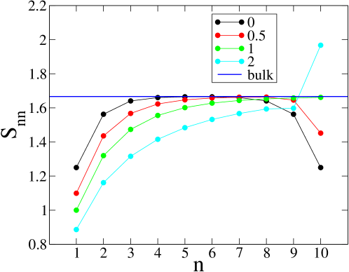
The most salient novel features of the process on an open chain, with respect to the geometry of a ring, appear clearly on the above expressions for small values of . The nonequilibrium stationary state now depends on the asymmetry parameter , and exhibits a non-trivial spatial dependence. This is illustrated in figure 2, showing the spatial profile of the spin strength for an open chain of sites with , so that the correlation length is , and several . In the case of a reversible process (), we have . The analytical result (4.2) is shown in black. As is increased, the spin strength profile becomes more and more asymmetric, and the trend to saturate to the thermodynamic value (4.4) is slower and slower. For , i.e., when has real spectrum, the spin strength is less than its thermodynamic value and decreases near the ends of the chain. For , i.e., when has complex spectrum, the spin strength exhibits a pronounced overshoot near the right end. Finally, for , i.e., when is lower triangular, the system does not ‘feel’ its right end. We shall come back to this totally asymmetric situation in section 4.7.
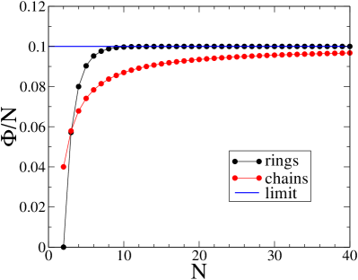
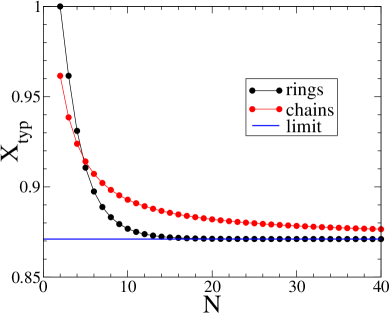
In spite of the above, intensive quantities characterising the nonequilibrium stationary state of the process on an open chain and on a ring converge to the same thermodynamic limits. This is illustrated in figure 3, showing the entropy production rate per spin (left) and the typical FDR (right) against system size up to 40 for rings (black) and open chains (red) in a typical situation ( and ). The thermodynamic limits (3.23) and (3.26) are shown as blue horizontal lines. The convergence is observed to be very fast in the case of rings, in agreement with the expected exponential convergence in . In the geometry of an open chain, extensive quantities are expected to possess a finite additive boundary contribution. In the case of the entropy production rate, this reads
| (4.22) |
up to exponentially small corrections in . Intensive quantities per spin are therefore expected to exhibit corrections. This explains the observed slow convergence.
4.6 The small- regime
In the regime where the asymmetry parameter is small, the entropy production rate vanishes quadratically. This behavior appears clearly on the expressions (4.17), (4.20) and (4.21) for the first few values of .
The entropy production amplitude
| (4.23) |
has been evaluated as a function of for all system sizes . The full derivation is given in A. We obtain (see (1.15))
| (4.24) |
For large enough systems, the above result assumes the form (see (4.22))
| (4.25) |
where the entropy production amplitude per spin (see (1.24))
| (4.26) |
agrees with (3.23), whereas the boundary contribution reads (see (1.25))
| (4.27) |
where and are the complete elliptic integrals. This boundary term is always negative. It diverges logarithmically as
| (4.28) |
as the critical point is approached ().
Right at the critical point, the entropy production amplitude scales as (see (1.29))
| (4.29) |
It is very plausible that the logarithmic terms in (4.28) and (4.29) are connected to each other by a finite-size scaling function of the dimensionless variable . As a first step in this direction, let us mention – without giving any detail – that we have been able to evaluate the finite part entering (4.29) and found
| (4.30) |
where is Euler’s constant.
4.7 The totally asymmetric case
In the borderline case , where interactions are totally asymmetric, the friction matrix is lower triangular. The Sylvester equation (4.7) simplifies to the recursion
| (4.31) |
whose solution reads
| (4.32) |
This expression is readily checked by inspection. It does not involve the system size explicitly. Indeed, as already observed on figure 2, the system does not ‘feel’ its right end.
Far from the left boundary, the translationally invariant correlations of the infinite system should be recovered. For and large, keeping the distance fixed, and setting , we indeed find that the expression (4.32) converges to
| (4.33) |
The entries of the antisymmetric matrix read
| (4.34) |
hence
| (4.35) |
Far from the left boundary, with the above conventions, we have for , and .
The entropy production rate reads (see (2.29))
| (4.36) |
where the dependence on the size is entirely contained in the summation bound. Using (4.35) and rearranging the sums, we obtain
| (4.37) |
This result can be readily brought to the form (4.22) for large chains. For the entropy production rate per spin , we obtain the very same series expansion (4.26) as in the small- regime. The expression (3.23) is thus recovered. For the boundary contribution, we obtain
| (4.38) |
This boundary term is always negative. It diverges linearly as the critical point is approached (), whereas its counterpart in the small- regime diverges only logarithmically (see (4.28)).
It is worth investigating the totally asymmetric case right at the critical point. The spin strength at site diverges with distance according to
| (4.39) |
This square-root divergence is however weaker than the linear growth of the spin strength in the bulk of the chain at criticality in the symmetric case (see (4.3)), i.e.,
| (4.40) |
The expression (4.37) for the entropy production rate can be recast as
| (4.41) |
Each correction term behaves asymptotically as , and so
| (4.42) |
Finally, the finite-size scaling law obeyed by the entropy production rate in the critical regime ( large and small) can also be evaluated. Simplifying the expression (4.37) for small, replacing sums by integrals, we indeed obtain
| (4.43) |
where, rather unexpectedly, the argument of the scaling function is , and not , which is the natural scaling variable. The scaling function is given by
| (4.44) |
For , the expansion
| (4.45) |
reproduces the critical behavior (4.42), with regular corrections. For , we have
| (4.46) |
The first term matches the leading behavior of the thermodynamic result (3.23), i.e., . The second term matches the divergence of the expression (4.38) of as . The third term shows that the leading correction to the asymptotic result (4.22) is indeed exponentially small.
5 Electrical arrays
Our second class of examples of multivariate Ornstein-Uhlenbeck processes originates in macroscopic physics. We shall consider arrays of resistively coupled and electrical circuits, where resistors are sources of thermal noise. Within this framework, irreversibility is brought about by an inhomogeneous temperature profile [46, 62]. Electrical circuits have been used in the past as a playground to test general ideas around the minimum and maximum entropy production principles [63, 64].
5.1 network
We first consider an array of resistively coupled circuits, as depicted in figure 4. All resistors and coils have the same resistance and inductance . The loop currents are denoted as (). In the most general situation, each resistor is kept at a different temperature ().
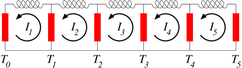
The total voltage drop around the loop traversed by the current reads
| (5.1) | |||||
According to the Johnson-Nyquist theory of thermal noise, the are independent Gaussian white noises obeying
| (5.2) |
The Dirichlet boundary conditions hold throughout section 5.
Equation (5.1) can be recast as
| (5.3) |
with
| (5.4) |
The above equations define an Ornstein-Uhlenbeck process of the form (2.1) in terms of the intensities . The friction matrix reads
| (5.5) |
where is (minus) the Laplacian on the chain. It is a symmetric tridiagonal Toeplitz matrix whose non-zero elements are
| (5.6) |
We remark that is twice the matrix giving the action of the critical Gaussian spin model on the open chain. As a consequence, the entries of its inverse read (see (4.3))
| (5.7) |
We have in particular
| (5.8) |
The diffusion matrix reads
| (5.9) |
where is the temperature matrix, whose non-zero elements can be worked out from (5.2) and (5.4):
| (5.10) |
As a consequence of the above, the Sylvester equation (2.15) reads
| (5.11) |
When all resistors are at the same temperature (), we have
| (5.12) |
the matrices and are proportional to each other, and the process is reversible, as expected. The covariance matrix reads
| (5.13) |
and so the loop intensities are independent and equally distributed Gaussian processes.
As recalled above, irreversibility is brought about by the spatial inhomogeneity of the temperature profile. Indeed, as soon as temperature is not homogeneous, the matrices and do not commute, the process is irreversible, and the Sylvester equation (5.11) for the covariance matrix is non-trivial. The case is however an exception: and commute and the process is reversible, even in the presence of an inhomogeneous symmetric temperature profile, such that (see below).
The main emphasis will again be on the entropy production rate . Furthermore, we are mostly interested in the regime where temperature fluctuations are small, i.e.,
| (5.14) |
In this regime, let us anticipate that the entropy production rate is given by a quadratic form of the temperature fluctuations, i.e.,
| (5.15) |
For the sake of clarity, the bounds of summations will be written down explicitly throughout this section 5. The amplitude matrix is dimensionless and only depends on the network size . It is a positive semi-definite matrix with dimension and rank (rank 1 for ).
In the special situation of a weakly disordered temperature profile, where the temperature fluctuations are independent and identically distributed random variables such that
| (5.16) |
with , the result (5.15) yields the following prediction for the mean entropy production rate:
| (5.17) |
with
| (5.18) |
It is worth having a closer look at the first few values of .
.
We have
| (5.19) |
The reversibility condition yields one single condition: . As a consequence, and commute and the process is reversible, even in the presence of an inhomogeneous symmetric temperature profile, such that . The Sylvester equation (5.11) yields
| (5.20) |
We have then
| (5.21) |
The entropy production rate reads, in full generality
| (5.22) |
When the temperature difference is small, this expression simplifies to
| (5.23) |
in agreement with the announced form (5.15), with
| (5.24) |
and therefore
| (5.25) |
.
We have
| (5.26) |
The general expressions for and are too lengthy to be reported here. The amplitude matrix
| (5.27) |
has rank 3 and trace
| (5.28) |
.
We shall only give the expressions of the amplitude matrix
| (5.29) |
and of its trace
| (5.30) |
For an arbitrary network size , the amplitude matrix entering the expression (5.15) of the entropy production rate has been derived in B.1. The outcome reads (see (2.11))
| (5.31) | |||||
The quantity can be worked out in more detail. We thus obtain
| (5.32) |
For a large network (), we have (see (4.22))
| (5.33) |
The intensive part is readily obtained by replacing the double sum in (5.32) by the corresponding integral. We thus get
| (5.34) |
The boundary contribution can be derived by means of a careful analysis of the difference between the double sum in (5.32) and the corresponding integral, using twice the first-order Euler-Maclaurin formula. We are left with
| (5.35) |
This quantity is negative, just as its counterparts (4.27) and (4.38) in the Gaussian spin model on an open chain. In all these cases, there is less entropy production near the ends of the sample than in its bulk.
To close, let us consider the situation where the temperature profile is homogeneous over the whole network (), except for the leftmost resistor, whose temperature is , with . We have then
| (5.36) |
For a large enough network (), the expression (5.31) for the amplitude approaches the limit
| (5.37) | |||||
The inequality confirms that the local entropy production rate is smaller near the boundaries.
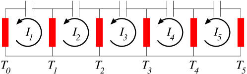
5.2 network
We now consider an array of resistively coupled circuits, as depicted in figure 5. All resistors and capacitors have the same values and . The loop currents read
| (5.38) |
where is the electric charge of the right electrode of the capacitor of circuit number . As in the previous case, each resistor is kept at a different temperature ().
The total voltage drop around the loop traversed by reads
| (5.39) | |||||
where the Johnson-Nyquist noises are still given by (5.2). The above equations can be recast as
| (5.40) |
with
| (5.41) |
The similarity between equations (5.3) and (5.40) demonstrates that the and networks are somehow dual to each other. The noise terms are proportional to each other, whereas time derivatives act on the left-hand side in (5.3), and on the right-hand side in (5.40).
Equations (5.40) can be brought to the canonical form (2.1) of a multivariate Ornstein-Uhlenbeck process in terms of the charges , by acting upon them by the inverse of the Laplacian . We thus obtain
| (5.42) |
At variance with the examples considered so far in this work, this process is non-local, in the sense that the corresponding matrices, i.e.,
| (5.43) |
are long-ranged. The temperature matrix is again given by (5.10). As a consequence of the above, the Sylvester equation (2.15) reads
| (5.44) |
The similarity between equations (5.11) and (5.44) yields a remarkable consequence of the above duality. If the and networks are subjected to the same temperature profile, their covariance matrices are proportional to each other, i.e.,
| (5.45) |
with obvious notations. The above symmetry however does not extend to all observables. In particular, there is no simple relationship between the entropy production rates of the two networks.
When all resistors are at the same temperature (), we have (see (5.12)), hence
| (5.46) |
Here again, the matrices and are proportional to each other, and the process is reversible, as expected. The covariance matrix reads
| (5.47) |
and so the charges are independent and equally distributed Gaussian processes.
The main quantities of interest will again be the entropy production rate in the regime where temperature fluctuations are small (see (5.14)), which now reads
| (5.48) |
where the amplitude matrix is again a dimensionless and positive semi-definite matrix, which only depends on size . In the special situation of a weakly disordered temperature profile (see (5.16)), this becomes
| (5.49) |
where again
| (5.50) |
Before we proceed, it is again worth looking at the first few values of .
.
The expression (5.7) yields
| (5.51) |
The reversibility condition again yields the single condition . The matrix is proportional to (5.20), in agreement with (5.45). We have then
| (5.52) |
The entropy production rate reads
| (5.53) |
When the temperature difference is small, has the form (5.48), with
| (5.54) |
and therefore
| (5.55) |
.
We shall only give the expression of the amplitude matrix
| (5.56) |
and of its trace
| (5.57) |
.
We shall only give the expression of the amplitude matrix
| (5.58) |
and of its trace
| (5.59) |
For an arbitrary network size , the amplitude matrix entering the expression (5.48) of the entropy production rate has been derived in B.2. The outcome reads (see (2.16))
| (5.60) | |||||
The quantity can be worked out in more detail. We thus obtain
| (5.61) |
Some algebra using the sum rule (5.8) yields
| (5.62) |
with
| (5.63) |
For a large network (), expanding the cosines to quadratic order, the latter sum can be estimated as
| (5.64) |
We thus obtain
| (5.65) |
The finite part is not predicted by this heuristic reasoning.
In the situation where the temperature profile is homogeneous except for the leftmost resistor, whose temperature is , with , we have
| (5.66) |
For a large network (), the expression (5.60) for can be analysed along the previous lines. We thus obtain
| (5.67) |
The entropy production rate exhibits an anomalous growth with the network size . In the case of a weakly disordered temperature profile, the amplitude grows quadratically (see (5.65)), whereas it grows linearly in the network (see (5.33)). In the case of a boundary temperature inhomogeneity, the amplitude grows linearly (see (5.67)), whereas it saturates to a constant value in the network (see (5.37)). These anomalous growth laws reflect a violation of extensivity which can be attributed to the peculiar feature of the present network, namely that the process is non-local, in the sense that the matrices and are long-ranged. As far as logarithmic subleading terms are concerned, they are due to the effective criticality of the model. Indeed, logarithmic corrections are also met in the regime of the critical open spin chain (see (4.28) and (4.29)), but not in the case of the network.
To close, let us mention – again without giving any detail – that we have evaluated the finite part and found
| (5.68) |
where is again Euler’s constant. Note the striking similarity with (4.30).
6 Discussion
This work was devoted to a characterisation of the nonequilibrium stationary state of a generic multivariate Ornstein-Uhlenbeck process involving degrees of freedom. The main advantage of this class of processes is that the linearity of the Langevin equations allows us to use linear algebra, and therefore to derive closed-form expressions for many quantities of interest.
The key point unifying the general results derived in section 2 is that the irreversibility of the process is characterised by a single antisymmetric matrix , which is nothing but the antisymmetric part of the Onsager matrix of kinetic coefficients (see (2.18)). All physical quantities characterising the nonequilibrium stationary state have been expressed either in terms of the matrix or of its associated Hermitian form (see (2.19)). These quantities include, most importantly, the entropy production rate (see (2.28), (2.29)), as well as the stationary probability current (see (2.23), (2.24)), the fluctuation-dissipation ratio matrix (see (2.39)) and typical fluctuation-dissipation ratio (see (2.42)), and the asymmetry index (see (2.20)).
Our first example of multivariate Ornstein-Uhlenbeck processes is the one-dimensional ferromagnetic Gaussian spin model endowed with a stochastic dynamics where spatial asymmetry results in irreversibility. This dynamics is the most general one keeping both the linearity and the range of interactions. Its parametrisation is inspired by earlier studies on directed Ising and spherical ferromagnets [25, 26, 29, 31, 55]. We successively investigated the model on a ring (section 3) and on an open chain (section 4). There is a qualitative difference between the two geometries. The stationary state of the model on a ring is independent of the asymmetry parameter , whereas it depends continuously on on an open chain. The independence of stationary-state spin correlations on in the ring geometry can be attributed to a symmetry: the process is cyclically symmetric. The very same property had been observed on the spherical model in the thermodynamic limit in any dimension [55]. There too, the independence of stationary correlations on the bias originates in translational invariance. The influence of symmetries on the stationary state of Gaussian and spherical models is by no means limited to the realm of stochastic dynamics. Let us mention a static analogue of the above. The well-known equivalence between the O Heisenberg model in the large- limit and the spherical model [65] only holds if the sample is a symmetric space, i.e., if all sites are equivalent. In other geometries, such as the open chain considered in the present work, the situation is more complex. The Heisenberg model indeed identifies, in the large- limit, with a generalised spherical model involving as many constraints as there are classes of inequivalent sites [66].
The general results obtained in section 2 allowed us to derive explicit expressions for the physical quantities characterising the nonequilibrium stationary state of the Gaussian spin model in the thermodynamic limit. All these results (see section 3.4) are independent of the geometry. Much attention has also been paid to finite-size effects, which are different in the ring and chain geometries, especially in the vicinity of the critical point. The main focus has been on the entropy production rate , which is both fundamental for the characterisation of a nonequilibrium stationary state, and the easiest to analyse. In the critical region on a ring, is the sum of an extensive part and of a finite-size contribution which is a function of the natural scaling variable , where is the inverse of the static correlation length. The situation on an open chain is more contrasted. First of all, is the sum of an extensive part and of a finite, negative boundary contribution (see (4.22)). The latter boundary term diverges as the critical point is approached, albeit in a non-universal fashion, namely logarithmically (either in or in ) in the regime of a small asymmetry (), and as a square-root of in the case of totally asymmetric interactions ().
For our second class of examples of multivariate Ornstein-Uhlenbeck processes, we have taken our inspiration from macroscopic physics. We have considered arrays of resistively coupled and electrical circuits. The main emphasis has been put on the entropy production rate in the situation where the local temperatures of the resistors are independent random variables with small fluctuations. As a general rule, there is less entropy production near the ends of the networks than in their bulk. Another salient outcome is the qualitatively different scaling of the entropy production rate in both cases. On networks (section 5.1), is again the sum of an extensive part and of a negative boundary contribution (see (5.33)). On networks (section 5.2), grows quadratically with , thus violating extensivity, with a large negative ‘non-local boundary’ contribution, growing as (see (5.65)).
Irreversible stochastic processes manifest yet another generic feature. Asymmetry is known to accelerate the dynamics of diffusions and other classes of processes [25, 26, 30, 32, 34, 57, 58, 59, 60, 61]. This phenomenon is however absent in most of the examples considered in this work. For the Gaussian spin model on a ring, this is because the process is cyclically symmetric. For the electrical networks, this is because of the symmetry of Kirchhoff’s laws. The above acceleration is therefore only observed in the ferromagnetic Gaussian model on an open chain (see (4.14)). We hope to come back to this acceleration mechanism in a more general setting in future work.
Appendix A Derivation of the expression (4.26) for the entropy production amplitude on the open spin chain
In this appendix we give a full derivation of the expression (4.26) for the entropy production amplitude of the spin model on an open chain in the regime where the asymmetry parameter is small. There, it is natural to expand quantities of interest as power series in . Setting (see (4.6))
| (1.1) |
we look for a solution to the Sylvester equation (2.15) in the form
| (1.2) |
We have , whose entries are given by (4.2), whereas obeys
| (1.3) |
We have then , where
| (1.4) |
The entropy production amplitude (see (4.23))
| (1.5) |
is given by (see (2.29))
| (1.6) |
In order to solve (1.3) for , it is convenient to introduce the following orthonormal basis of the space of matrices (see (4.11))
| (1.7) |
where the quantised momenta fit to Dirichlet boundary conditions read
| (1.8) |
An arbitrary matrix can be expanded as
| (1.9) |
With these notations, we have
| (1.10) |
where
| (1.11) |
are the eigenvalues of (see (4.13)). Moreover (see (4.6))
| (1.12) |
where the quantisation of the momenta automatically takes boundary conditions into account. The sum over can be reduced to geometric sums. We thus obtain
| (1.13) |
while these amplitudes vanish if the sum is even. The solution to (1.3) reads
| (1.14) |
Some algebra using the above results yields the explicit expression
| (1.15) |
Some more work is still needed in order to extract the size dependence of this result in a form similar to (4.22). In a first step, introducing the odd integers and , as well as the angles
| (1.16) |
we can recast (1.15) as
| (1.17) |
where each odd integer or runs over values between 1 and . In a second step, expanding (1.17) as a power series in (i.e., a high-temperature series) yields
| (1.18) |
with
| (1.19) |
The latter sums enjoy a few simplifying features. First, the recurrence formula , with initial value (see [56, Eq.(24.1.1)])
| (1.20) |
allows us to express the in terms of the . Second, for large enough, the sum is exactly given by the product of the corresponding normalised integral,
| (1.21) |
and of the number of terms, i.e., . This is a consequence of the Poisson summation formula. We thus obtain
| (1.22) |
The above estimate is sufficient to obtain a result of the form (4.22) for the entropy production amplitude on a large open chain, i.e.,
| (1.23) |
The entropy production amplitude per spin reads
| (1.24) |
in agreement with (3.23), as . The boundary contribution reads
| (1.25) | |||||
where and are the complete elliptic integrals. The boundary term is always negative. It diverges logarithmically as
| (1.26) |
as the critical point is approached ().
Right at the critical point, the result (1.18) simplifies to
| (1.27) |
Moreover, the large- behavior of the estimate (1.22), i.e.,
| (1.28) |
holds up to values of comparable to , beyond which the sums fall off exponentially fast, as . We thus obtain
| (1.29) |
The finite part is not predicted by the above line of reasoning.
Appendix B Derivation of the expressions (5.31) and (5.60) for the amplitude matrices of the and arrays
In this appendix we give a full derivation of the expressions (5.31) and (5.60) for the amplitude matrices of the and electrical networks investigated in section 5, for an arbitrary network size .
B.1 networks (see section 5.1)
The derivation of the amplitude matrix entering (5.15) goes as follows. The expression (5.10) of the temperature matrix can be recast as
| (2.1) |
where the non-zero elements of the matrix are
| (2.2) |
Along the lines of section 4.6, let us evaluate the matrices and to first order in , i.e., to first order in the temperature fluctuations . Looking for a solution to the Sylvester equation (5.11) of the form
| (2.3) |
we find that the matrix obeys
| (2.4) |
We have then
| (2.5) |
Finally, using (2.29), we obtain the following expression
| (2.6) |
for the entropy production rate to the required accuracy, i.e., to second order in the temperature fluctuations .
In order to solve (2.4) for , it is convenient to use the same formalism as in A, including the quantised momenta (1.8) and the orthonormal basis introduced in (1.7). Within these conventions, we have
| (2.7) |
whereas (2.2) yields after some algebra
| (2.8) |
The solution to (2.4) then reads
| (2.9) |
As a consequence, (2.6) can be recast as
| (2.10) |
Finally, using (2.8), this expression can be brought to the announced form (5.15), where the entries of the amplitude matrix read
| (2.11) | |||||
B.2 networks (see section 5.2)
The derivation of the amplitude matrix entering (5.48) follows the same lines. The duality symmetry (5.45) implies that the covariance matrix is given by
| (2.12) |
where the matrices and are the same as in B.1, whereas (2.5) and (2.6) respectively become
| (2.13) |
and
| (2.14) |
Using (2.9), the latter expression can be recast as
| (2.15) |
Finally, using (2.8), this expression can be brought to the announced form (5.48), where the entries of the amplitude matrix read
| (2.16) | |||||
References
References
- [1] Gallavotti G and Cohen E G D 1995 J. Stat. Phys. 80 931
- [2] Eyink G L, Lebowitz J L and Spohn H 1996 J. Stat. Phys. 83 385
- [3] Kurchan J 1998 J. Phys. A 31 3719
- [4] Crooks G E 1999 Phys. Rev. E 60 2721
- [5] Lebowitz J L and Spohn H 1999 J. Stat. Phys. 95 333
- [6] Maes C, Redig F and Van Moffaert A 2000 J. Math. Phys. 41 1528
- [7] Seifert U 2005 Phys. Rev. Lett. 95 040602
- [8] Derrida B 2007 J. Stat. Mech. P07023
- [9] Marconi U M B, Puglisi A, Rondoni L and Vulpiani A 2008 Phys. Rep. 461 111
- [10] Touchette H 2009 Phys. Rep. 478 1
- [11] Seifert U 2012 Rep. Prog. Phys. 75 126001
- [12] Uhlenbeck G E and Ornstein L S 1930 Phys. Rev. 36 823
- [13] Wang M C and Uhlenbeck G E 1945 Rev. Mod. Phys. 17 323
- [14] Lax M 1960 Rev. Mod. Phys. 32 25
- [15] Lax M 1966 Rev. Mod. Phys. 38 359
- [16] Risken H 1984 The Fokker-Planck Equation: Methods of Solution and Applications (Berlin: Springer)
- [17] van Kampen N G 1992 Stochastic Processes in Physics and Chemistry (Amsterdam: North-Holland)
- [18] Gardiner C W 2004 Handbook of Stochastic Methods for Physics, Chemistry, and Natural Sciences Springer Series in Synergetics (Berlin: Springer)
- [19] Graham R and Tél T 1984 Phys. Rev. Lett. 52 9
- [20] Ao P 2004 J. Phys. A 37 L25
- [21] Kwon C, Ao P and Thouless D J 2005 Proc. Nat. Acad. Sci. USA 102 13029
- [22] Qian H, Qian M and Tang X 2002 J. Stat. Phys. 107 1129
- [23] Künsch H R 1984 Z. Wahr. verw. Gebiete 66 407
- [24] Lima F W S and Stauffer D 2006 Physica A 359 423
- [25] Godrèche C and Bray A J 2009 J. Stat. Mech. P12016
- [26] Godrèche C 2011 J. Stat. Mech. P04005
- [27] de Oliveira M J 2011 J. Stat. Mech. P12012
- [28] de Oliveira M J 2013 J. Stat. Mech. E04001
- [29] Godrèche C 2013 J. Stat. Mech. P05011
- [30] Godrèche C and Pleimling M 2014 J. Stat. Mech. P05005
- [31] Godrèche C and Luck J M 2015 J. Stat. Mech. P05033
- [32] Godrèche C and Pleimling M 2015 J. Stat. Mech. P07023
- [33] Godrèche C and Luck J M 2017 J. Stat. Mech. 073208
- [34] Godrèche C and Pleimling M 2018 J. Stat. Mech. 043209
- [35] Tomita K and Tomita H 1974 Prog. Theor. Phys. 51 1731
- [36] Brander K and Seifert U 2013 New J. Phys. 15 105003
- [37] Macieszczak K, Brandner K and Garrahan J P 2018 Phys. Rev. Lett. 121 130601
- [38] Prigogine I 1961 Introduction to Thermodynamics of Irreversible Processes (New York: Wiley)
- [39] de Groot S R and Mazur P 1962 Non-Equilibrium Thermodynamics (Amsterdam: North-Holland)
- [40] Qian M P, Qian M and Gong G L 1991 Contemp. Math. 118 255
- [41] Qian M and Wang Z D 1999 Commun. Math. Phys. 206 429
- [42] Qian H 2001 Proc. Roy. Soc. London A 457 1645
- [43] Zhang F and Qian M 2007 Acta Math. Sci. 27 B 145
- [44] Qian H 2013 J. Math. Phys. 54 053302
- [45] Tomé T and de Oliveira M J 2013 Phys. Rev. E 82 021120
- [46] Landi G T, Tomé T and de Oliveira M J 2013 J. Phys. A 46 395001
- [47] Spinney R E and Ford I J 2012 Phys. Rev. E 85 051113
- [48] Corberi F, Lippiello E and Zannetti M 2007 J. Stat. Mech. P07002
- [49] Leuzzi L 2009 J. Non-Cryst. Solids 355 686
- [50] Cugliandolo L F 2011 J. Phys. A 44 483001
- [51] Cugliandolo L F and Kurchan J 1994 J. Phys. A 27 5749
- [52] Basu U, Maes C and Netocny K 2015 New J. Phys. 17 115006
- [53] Berlin T H and Kac M 1952 Phys. Rev. 86 821
- [54] Hase M O and de Oliveira M J 2012 J. Phys. A 45 165003
- [55] Godrèche C and Luck J M 2013 J. Stat. Mech. P05006
- [56] Hansen E R 1975 A Table of Series and Products (Englewood Cliffs, NJ, USA: Prentice-Hall)
- [57] Hwang C R, Hwang-Ma S Y and Sheu S J 1993 Ann. Appl. Prob. 3 897
- [58] Hwang C R, Hwang-Ma S Y and Sheu S J 2005 Ann. Appl. Prob. 15 1433
- [59] Lelièvre T, Nier F and Pavliotis G A 2013 J. Stat. Phys. 152 237
- [60] Wu S J, Hwang C R and Chu M T 2014 J. Stat. Phys. 155 571
- [61] Kaiser M, Jack R L and Zimmer J 2017 J. Stat. Phys. 168 259
- [62] Bruers S, Maes C and Netocny K 2007 J. Stat. Phys. 129 725
- [63] Landauer R 1975 Phys. Rev. A 12 636
- [64] Landauer R 1975 J. Stat. Phys. 13 1
- [65] Stanley H E 1968 Phys. Rev. 176 718
- [66] Knops H J F 1973 J. Math. Phys. 14 1918