Polarimetric and spectroscopic study of radio-quiet weak emission line quasars

Abstract

A small subset of optically selected radio-quiet quasars showing weak or no emission lines may turn out to be the elusive radio-quiet BL Lac objects, or simply be radio-quiet QSOs with a still-forming/shielded broad line region (BLR). High polarisation ($p$ $>$ 3$-$4$\%$), a hallmark of BL Lacs, can be used to test whether some optically selected ‘radio-quiet weak emission line quasars’ (RQWLQs) show a fractional polarisation high enough to qualify as radio-quiet analogs of BL Lac objects. Out of the observed six RQWLQs candidates showing an insignificant proper motion, only two are found to have $p$ $>$ 1$\%$. For these two RQWLQs, namely J142505.59$+$035336.2, J154515.77+003235.2, we found polarisation of 1.03$\pm$0.36$\%$, 1.59$\pm$0.53$\%$ respectively, which again is too modest to justify a (radio-quiet) BL Lac classification. We also present here a statistical comparison of the optical spectral index, for a set of 40 RQWLQs with redshift-luminosity matched control sample of 800 QSOs and an equivalent sample of 120 blazars. The spectral index distribution of RQWLQs is found to differ, at a high significance level, from that of blazars and is consistent with that of the ordinary QSOs. Likewise, a structure-function analysis of photometric light curves presented here suggests that the mechanism driving optical variability in RQWLQs is similar to that operating in QSOs and different from that of blazars. These findings are consistent with the common view that the central engine in RQWLQs, as a population, is akin to that operating in normal QSOs and the primary differences between them might be related to differences in the BLR.

1 Introduction

BL Lac objects are characterized by a large flux variability from radio-to-TeV frequencies, nearly featureless optical spectrum and in many cases superluminal motion of the nuclear radio blobs (Urry & Padovani, 1995, and reference therein). They also have a compact core-dominated radio morphology and usually a high ($>$ 3$\%$) and variable polarisation at radio-to-optical frequencies. Such observed properties of BL Lac are well explained by a model in which the dominant source of the observed emission is a relativistic jet of radiating plasma directed within a small angle to our line of sight, as envisioned in the unification scheme of active galactic nuclei (AGN) (e.g., Begelman et al., 1984; Urry & Padovani, 1995; Antonucci, 2012).

Traditionally, BL Lac objects have been discovered from radio and X-ray surveys. The two populations of BL Lacs (radio-selected, RBL, or X-ray selected, XBL) are known to have significant differences in parameters, such as the frequencies of the peaks in the Spectral Energy Distribution (SED) (e.g, Padovani & Giommi, 1995) and optical fractional polarisation, $p$ (e.g, Jannuzi et al., 1994). Compared to XBLs, the RBLs show more prominent radio cores, stronger polarisation and flux variability, as well as relatively higher luminosities in the radio and optical. It is presently unknown if there exists a subset of BL Lacs which is radio-quiet, by analogy to the abundant population of radio-quiet quasars. Stocke et al. (1990) noted that unlike the radio dichotomy of quasars, there is no evidence for populations of BL Lac objects distinguished by radio loudness. Contrary to the traditional radio and X-ray surveys for BL Lac objects, optical surveys for radio-quiet weak-line quasars (RQWLQs) can, in principle, provide a more effective check on the existence of radio-quiet BL Lac objects, besides yielding a more complete census of the BL Lac population as a whole. The existence of such radio-quiet BL Lacs, if any, could also provide powerful constraints on the models of jet formation in AGN.

The Sloan Digital Sky Survey (SDSS; Collinge et al., 2005) and the Two Degree Field QSO Redshift Survey (2QZ; Londish et al., 2002) resulted in the first optically selected samples of BL Lac candidates, with 386 candidates coming from the SDSS and 56 from the 2QZ. Since then, Plotkin et al. (2010a) have derived a larger sample of 723 optically selected BL Lac candidates using the SDSS Data Release 7 (DR-7, Abazajian et al., 2009). Majority of the objects in these samples of BL Lac candidates have weak broad emission-lines with a rest-frame EW $<15.4$ Å for the Ly$\alpha$$+$Nv emission-line complex  (Diamond-Stanic et al., 2009) and $<11$ Å , $<4.8$ Å  for the Mg ii and C iv, respectively (Meusinger & Balafkan, 2014). These have been termed as weak line quasars (WLQs), however the physical cause of their abnormally weak emission lines is still debated (see, e.g., Nicastro et al., 2003; Stalin & Srianand, 2005; Diamond-Stanic et al., 2009; Elitzur & Ho, 2009; Hryniewicz et al., 2010; Plotkin et al., 2010b; Laor & Davis, 2011; Liu & Zhang, 2011; Nikołajuk & Walter, 2012). One possible explanation for the abnormality is that the covering factor of the broad-line region (BLR) in WLQs could be at least an order-of-magnitude smaller compared to that in normal QSOs (e.g. Nikołajuk & Walter, 2012). An extreme version of this scenario is that in WLQs the accretion disk is relatively recently established and hence a significant BLR is yet to develop (Hryniewicz et al., 2010; Liu & Zhang, 2011). A yet another possibility is a high mass of the central BH (M${}_{BH}>~{}3\times 10^{9}M_{\odot}$) which can result in an accretion disk which is too cold to emit sufficient number of UV ionizing photons, even when its optical output is high (Laor & Davis 2011, also, Plotkin et al. 2010a).

While the above mentioned limited empirical evidence and theoretical scenarios are consistent with the bulk of the RQWLQs population being a special case of the standard radio-quiet quasars, they do not rule out the possibility that a small subset of this population may in fact be the long-sought radio-quiet BL Lac objects in which optical emission does arise predominantly from a relativistic jet of synchrotron radiation (e.g, Stocke & Perrenod, 1981; Stalin & Srianand, 2005; Diamond-Stanic et al., 2009; Plotkin et al., 2010a). One strategy to pursue such a search is to characterize the optical polarisation and intra-night optical variability (INOV) of RQWLQs. These are the two main characteristic properties of BL Lac objects; namely an optical polarisation, $p$ $>$ 3% (e.g., Heidt & Nilsson, 2011) and an INOV duty cycle approaching the level of $\sim$50 percent (at an INOV amplitude $\psi>3$%) (e.g, Gopal-Krishna et al., 2003; Sagar et al., 2004; Stalin et al., 2004a, b; Gopal-Krishna et al., 2011; Goyal et al., 2012). To characterize INOV of RQWLQs, our group has recently analysed a sample of $70$ intranight light curves of $34$ RQWLQs (Gopal-Krishna et al., 2013; Chand et al., 2014; Kumar et al., 2015, 2016, 2017) and reported that two of the RQWLQs in two separate sessions exhibited strong INOV with $\psi>$ 10%, like that of BL Lacs, though the duty cycle of INOV was found to be only about $\sim 5\%$ which is typical of normal radio-quiet QSOs (Kumar et al. 2017, and references therein, see also Liu et al. 2015). On the other hand, efforts for a systematic polarimetric characterization of radio-quiet BL Lac candidates have been quite limited, although polarimetric surveys have been reported for WLQs in general  (e.g, Smith et al., 2007; Heidt & Nilsson, 2011). Therefore it seems worthwhile to investigate a sub-sample of optically selected WLQs whose members have (i) a radio-loudness parameter (R) $<10$, to ensure radio-quietness and (ii) a secure redshift measurement, or at least a proper motion consistent with zero. The proper motion check is particularly relevant for WLQs in view of the weakness or near absence of features in their spectra, which often renders their redshift estimates fairly uncertain. For such a sample of RQWLQs (see Sect. 2), we present here polarimetric and spectroscopic observations taken with the European Southern Observatory (ESO) 3.6m telescope at La Silla, Chile. Our main goal is four-fold: (i) with the new spectroscopic observations of our RQWLQ sample, we aim to constrain the emission redshifts based on any weak emission feature(s) that might show up in case the source happens to be in a low state on account of a weak continuum boosting, (ii) to investigate spectral properties such as the distribution of spectral slope, for comparison with the control samples of blazars and normal QSOs, (iii) to test whether any of the RQWLQs show a strong polarisation like the classical BL Lacs for which $p>3-4\%$ typically; this would establish them as a bona-fide radio-quiet counterpart of BL Lacs, and (iv) to investigate the long-term optical variability of these RQWLQs, for comparison with blazars and normal QSOs.

This paper is organized as follows. Sect. 2 describes our sample of RQWLQs and the polarimetric/spectroscopic observations, while Sect. 3 gives details of the data reduction and analysis. In Sect. 4, we present our results on the spectral and polarisation properties and the long-term optical variability of the RQWLQs and a comparison with those already established for blazars and QSOs. A brief discussion of our results followed by conclusions is presented in Sect. 5.

Table 1: The observed sample (see text).

SDSS Name	RA (J2000)	DEC(J2000)	$m_{R}$	PM.	$z_{emi}$	Obs. Date	Exp. Time
	(h m s)	(∘ ′ ′′)	(mag)	(mas/yr)		Spec.(Pol.)	(sec)
(1)	(2)	(3)	(4)	(5)	(6)	(7)	(8)
J100253.23$-$001727.0	10:02:53.23	$-$00:17:27.00	19.13	101.46$\pm$0.83		2006.04.24(26)	1200x3
J102615.30$-$000630.2	10:26:15.30	$-$00:06:30.22	19.26	52.62$\pm$1.37		2006.04.24(27)	1200x3
J103607.52$+$015659.0	10:36:07.52	$+$01:56:59.05	18.80	0.56$\pm$0.58	1.8768$\pm 0.0014^{\dagger}$	2006.04.24(26)	1200x3
J104519.72$+$002614.3	10:45:19.72	$+$00:26:14.38	18.63	64.81$\pm$0.65		2006.04.25(27)	600x3
J105355.17$-$005537.7	10:53:55.17	$-$00:55:37.72	19.41	17.92$\pm$1.12		2006.04.25(26)	1500x3
J113413.48$+$001042.0	11:34:13.48	$+$00:10:42.05	18.44	0.25$\pm$1.07	1.4857$\pm 0.0007^{\dagger}$	2006.04.24(27)	600x3
J114554.87$+$001023.9	11:45:54.87	$+$00:10:23.96	19.54	16.71$\pm$1.14		2006.04.25(27)	1800x3
J114521.64$-$024757.4	11:45:21.64	$-$02:47:57.48	18.65	14.85$\pm$0.89		2006.04.24(27)	600x3
J115909.61$-$024534.6	11:59:09.61	$-$02:45:34.65	19.02	0.64$\pm$0.83	2.0136$\pm 0.0006^{\dagger}$	2006.04.25(26)	1200x3
J120558.27$-$004217.8	12:05:58.27	$-$00:42:17.82	18.75	111.95$\pm$0.84		2006.04.24(27)	900x3
J120801.84$-$004218.3	12:08:01.84	$-$00:42:18.31	19.05	25.37$\pm$1.02		2006.04.25(27)	600x3
J122338.05$-$015617.1	12:23:38.05	$-$01:56:17.14	19.11	28.15$\pm$0.83		2006.04.25(..)	1200x3
J123437.64$-$012951.9	12:34:37.64	$-$01:29:51.94	19.18	0.98$\pm$1.27	1.7105$\pm 0.0003^{\ddagger}$	2006.04.25(27)	1200x3
J125435.81$-$011822.0	12:54:35.81	$-$01:18:22.03	19.15	19.97$\pm$0.94		2006.04…(28)
J130009.93$-$022559.2	13:00:09.93	$-$02:25:59.27	18.90	87.82$\pm$0.70		2006.04.24(..)	1200x3
J140916.33$-$000011.3	14:09:16.33	$-$00:00:11.31	18.65	38.76$\pm$0.64		2006.04.24(..)	600x3
J141046.75$-$023145.3	14:10:46.75	$-$02:31:45.35	18.13	22.06$\pm$1.66		2006.04.24(27)	1200x3
J142505.59$+$035336.2	14:25:05.59	$+$03:53:36.23	18.74	0.11$\pm$0.76	2.2353$\pm 0.0012^{\ddagger}$	2006.04.25(28)	600x3
J154515.77$+$003235.2	15:45:15.77	$+$00:32:35.26	18.82	0.22$\pm$0.70	1.0511$\pm 0.0005^{\dagger}$	2006.04.24(25)	1200x3
						2006.04.24(25)	1200x3

2 The Sample and Observations

In Table 1 of their paper, Londish et al. (2002) have given a sample of 56 objects derived from the 2QZ QSO survey on the criteria of a featureless optical spectrum and non-significant proper motion. Likewise, Collinge et al. (2005) used the SDSS to extract 386 optically selected BL Lac candidates. Out of these total 442 WLQs we extracted a set of 111 WLQs (88 out of the 386 and 23 out of the 56 candidates) for polarimetry/spectroscopy, by limiting to (i) 8-17h right ascension range, and (ii) m${}_{R}<20$-mag. Since our observations were scheduled for April, we trimmed our list from 111 to 19 RQWLQs, as listed in Table 1, by accepting only those lying within the 10-15h range in right ascension and at sufficiently low declination for ESO La Silla observatory, and also brighter than 19.5-mag in R-band ($m_{R}$), as well as lacking any published polarisation measurement (except for two sources). Moreover, the selected 19 RQWLQs either have a radio-loudness parameter R $<$ 10 (see, Kellermann et al., 1989), or a non-detection in the FIRST survey (i.e., somewhat conservatively, $<$ 1 mJy at 1.4 GHz, see Becker et al. 1995). Fifteen of these 19 RQWLQs could be covered in both our polarimetric and spectroscopic observations, 3 in spectroscopy alone, and one in polarimetry alone (see Table  1). These observations were carried out during 24-28 April, 2006 with the ESO 3.6m telescope at La Silla, equipped with the ESO Faint Object Spectrograph and Camera  (EFOSC; Buzzoni et al., 1984).

Details of the sample of 19 RQWLQs and the observation log are given in Table 1. The first four columns list the source name, right ascension (RA), declination (DEC) and magnitude in R-band ($m_{R}$). Since, for the present purpose we are only interested in genuine QSOs we shall subject the sample of 19 RQWLQ candidates to additional checks based on the latest proper motion data from Gaia measurements: DR2 (Gaia Collaboration et al., 2016, 2018). This is important since some classes of white dwarfs also display essentially feature-less optical spectra, but due to their association with the galactic halo population, they are very likely to have a finite proper motion. Indeed, 13 out of our 19 sources are now found to exhibit a non-zero proper motion, based on the Gaia/DR2. All 13 are henceforth discounted as RQWLQ candidates. The genuineness of the remaining 6 candidates as RQWLQ (with zero proper motion) is further confirmed by the availability in the literature of accurate, spectroscopically determined redshifts (all of which are above z $>$1.0, see Table 1). Our polarimetric and spectroscopic observations using the ESO 3.6m telescope are presented below for all these 6 RQWLQs. The last two columns of Table 1 give the observation dates (for spectroscopy and polarimetry) and the exposure time (for spectroscopy).

In addition, for making a statistical comparison of the optical spectral index and variability behavior of RQWLQs with those found for blazars and normal QSOs, we have enlarged the RQWLQ sample by adding the well-defined sample of 34 optically selected RQWLQs which has been derived from Plotkin et al. (2010a) and  Meusinger & Balafkan (2014) and being followed up under a separate program to determine their INOV characteristics (for details, see Kumar et al., 2015).

3 Data Reduction And Analysis

The polarimetric and spectroscopic observations were carried out during 24-28 April 2006 at ESO La Silla, Chile, using the 3.6m telescope equipped with EFOSC (Buzzoni et al., 1984), under the observation ID 077.B-0822(A) (Table 1). The detector system consists of ESO $\#40$ CCD, a Loral/Lesser Thinned, AR coated, UV flooded, MPP 2048 $\times$ 2048 chip, with a pixel size of 15 µm, corresponding to 0.12 arcsec/pixel on the sky. A chip with a readout noise of $7.8e^{-}$ and a gain of $0.91e^{-}$/ADU. CCD was used with Bessel -R(#642) filter. Spectroscopic observations of $18$ out of our total 19 sources (excluding J125435.81$-$011822.0) were performed with the EFOSC using Grism 6 and with a slit width of 1.0 arcsec. Grism 6 provides a wavelength coverage from $3860-8070$ Å with a wavelength dispersion of $2.06$ Å/pixel and FWHM of around 16.7 Å (at 1″slit-width) resulting in spectral resolution of about $\sim$400 (at 6000Å).

Firstly, all the raw images were corrected for bias subtraction, flat-fielded and subjected to cosmic-ray removal, using the standard tasks given in the data reduction software package IRAF . The raw two-dimensional data were reduced with the standard procedures using IRAF. The IRAF task $apall$ was used to extract the spectra. We then carried out the wavelength and flux calibration using the He-Ar lamp spectra and the standard stars, respectively. Exposure time for our spectroscopic observations ranges between 600 to 1800 sec, depending on faintness of the object, as listed in the last column of Table 1. We observed each source in three exposures and finally combined them to improve the SNR.

Polarimetric observations for 16 (including the 6 genuine RQWLQs discussed above) out of our total sample of $19$ sources were carried out through a Bessel-R filter in the polarimetric mode; i.e., a Wollaston prism and a half-wave plate were inserted into the beam, resulting in ordinary and extraordinary images of each target on the CCD chip, separated by $10$ arcsec. An unpolarised standard star was also observed for measuring the instrumental polarisation. Seeing during the observations was close to 1 arcsec. Fluxes of the ordinary and extraordinary images were measured by aperture photometry using the IRAF task $phot$, for all four position angles of the Wollaston prism viz 0^∘, 22.5^∘, 45^∘ and 67.5^∘. Stokes parameters (U, Q), percentage polarisation ($p$) and polarisation angle (PA) were then calculated using the following standard equations:

$$F(\beta_{i})=\frac{f^{o}(\beta_{i})-f^{e}(\beta_{i})}{f^{o}(\beta_{i})+f^{e}(\beta_{i})}$$ (1)

where $\beta_{i}$ = 22.5^∘ $\times$ ( i - 1) with i = 1, 2, 3, 4 and $f^{o}(\beta_{i})$ and $f^{e}(\beta_{i})$ are the fluxes measured for the ordinary and the extraordinary images. The parameters Q, U, $p$ and PA are given by :

$$Q=\frac{F(\beta_{1})-F(\beta_{3})}{2},\hskip 12.80365ptU=\frac{F(\beta_{2})-F(\beta_{4})}{2}$$ (2)

$$p=\sqrt{Q^{2}+U^{2}}$$ (3)

$$PA=\left\{\,{}{}\vbox{\halign{\relax\begingroup\csname @IEEEeqnarraycolPREl\endcsname#\relax\relax\relax\relax\relax\relax\relax\relax\relax\relax\csname @IEEEeqnarraycolPOSTl\endcsname\relax\relax\relax\relax\relax\relax\relax\relax\relax\relax\endgroup&\relax\begingroup\csname @IEEEeqnarraycolPREs\endcsname#\relax\relax\relax\relax\relax\relax\relax\relax\relax\relax\csname @IEEEeqnarraycolPOSTs\endcsname\relax\relax\relax\relax\relax\relax\relax\relax\relax\relax\endgroup&\bgroup#\egroup\cr$\displaystyle\mbox{\vrule width=0.0pt,height=8.39996pt,depth=3.60004pt}\frac{1}{2}tan^{-1}(\frac{U}{Q})$\hfil&U $\textgreater$ 0, Q $\textgreater 0$\hfil&{\vrule width=0.0pt,height=0.0pt,depth=0.0pt{}}\cr\vskip 3.0pt\vskip 0.0pt\cr$\displaystyle$90${}^{\circ}$+$\frac{1}{2}tan^{-1}(\frac{U}{Q})$\hfil&U $\textless$ 0, Q $\textgreater 0$ \hfil&{\vrule width=0.0pt,height=0.0pt,depth=0.0pt{}}\cr\vskip 3.0pt\vskip 0.0pt\cr$\displaystyle$90${}^{\circ}$+$\frac{1}{2}tan^{-1}(\frac{U}{Q})$\hfil&U $\textless$ 0, Q $\textless 0$ \hfil&{\vrule width=0.0pt,height=0.0pt,depth=0.0pt{}}\cr\vskip 3.0pt\vskip 0.0pt\cr$\displaystyle$180${}^{\circ}$+$\frac{1}{2}tan^{-1}(\frac{U}{Q})$\hfil&U $\textgreater$ 0, Q $\textless 0$ \mbox{\vrule width=0.0pt,height=8.39996pt,depth=3.60004pt}\hfil&{\vrule width=0.0pt,height=0.0pt,depth=0.0pt}\crcr}}\right.$$ (4)

4 Results

4.1 Spectroscopic Properties of RQWLQs

The motivation behind the present sensitive spectroscopic observations was not only to measure the spectral shape but also try to determine/constrain redshift by detecting some weak spectral features (either absorption or emission), particularly if the object happened to be in a faint state when the optical continuum is not strongly Doppler boosted. The reduced spectra for our $6$ RQWLQs are shown in Fig. 1. The spectra of the remaining 12 sources in our sample, whose extra-galactic origin now seems very unlikely in view of the significant proper motion, revealed recently by Gaia/DR2, will be presented elsewhere.

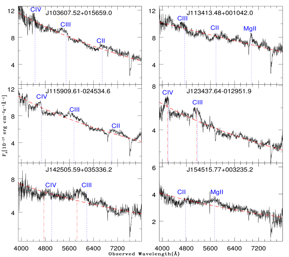
Figure 1: Spectra of our six sources having either zero or insignificant proper motion. The present ESO spectra are shown in solid line (black), while the spectral fit by a dashed line (red).The small dashed lines (blue) mark the positions of the expected emission lines based on the SDSS redshifts, while long dashed lines (red) correspond to the new redshifts based on our ESO spectra. We note that absorption features around 6900Å and 7600Å are tellric absorption features due to the earth’s atmosphere.

The redshifts of all the 6 genuine RQWLQs listed in Table 1 are based on their SDSS spectra. To assess the reliability of these existing redshifts, we have marked in Fig. 1 the positions of the expected centroid of various emission lines on our ESO 3.6m spectra. As can be seen from this figure, the features in our ESO 3.6m spectra are consistent with the SDSS redshifts for these 6 RQWLQs. We note here that the typical accuracy of the redshift determination will depend on the spectral resolution as well as the SNR. The resolution of the SDSS spectra is about 2000, which is almost 5 times higher than the resolution of our 3.6m ESO spectra, though in the latter case SNR is much better. Furthermore, we have noticed that out of our 6 RQWLQs, the SDSS redshifts of 4 sources have already been improved by Hewett & Wild (2010). For these sources redshift estimation could not be improved further using our ESO spectra. The SDSS redshift of the remaining two sources viz. J123437-012951, J142505+035336 (which were not covered in the Hewett & Wild (2010) redshifts determination), have been constrained here using our ESO spectra. For instance, our higher SNR ESO spectrum of J123437-012951 revealed clear signatures of two emission lines close to $\sim$4200Å and $\sim$5200Å. We use the publicly available template of composite SDSS spectra (after appropriate convolution and re-binning to match with our lower resolution ESO spectra) to determine the redshift of this source based on the template shifting procedure described in Bolton et al. (2012). As can be seen from the middle right panel of Fig. 1, our best-fit redshift of 1.6948$\pm$0.009 is very close to the redshift measured from the SDSS spectrum of this source. However, for J142505+035336 our new redshift measurement of 2.0664$\pm$0.0017 using our 3.6m ESO spectrum (based on the above template fitting technique) is found to be significantly different from its SDSS redshift (i.e. 2.2353$\pm$0.0012). In summary, our higher SNR spectroscopic observations (though with a smaller spectral resolution) have allowed us (i) to reconfirm the spectroscopic redshift measurement (based on low SNR but a higher spectral resolution) for 4 of our RQWLQs, (ii) to achieve a moderate improvement in redshift for the remaining two RQWLQs, besides proving useful for computing their best-fit power-law spectral slopes.

For fitting the spectral slope, we employed the Levenberg-Marquardt least-squares minimization technique (the MPFIT package, Markwardt, 2009). In this fitting, we have fitted a power-law function of the form $\lambda^{\alpha}$, to describe the AGN continuum emision. Fig. 1 shows our spectral fits for the $6$ RQWLQs.

The spectral fitting results enable a statistical comparison of the spectral slope distribution found for the RQWLQs with those for the control samples of normal QSOs and blazars. To enlarge the RQWLQ sample for this purpose, we have included another 34 well defined RQWLQs from Kumar et al. (2015) for which SDSS spectra are also available. We also noted that SDSS spectra are available also for the 6 RQWLQs of the present sample. So for the sake of homogeneous analysis, we have used SDSS spectra for computing the spectral slopes of all these 40 RQWLQs. To build a control sample of normal QSOs, we selected 20 QSOs from SDSS (York et al., 2000) for each of the $40$ RQWLQs, matched in redshift to within $\mid\Delta z\mid$ $<$ 0.005 and in r-band magnitude to within $\mid\Delta m\mid$ $<$ 0.1, together resulting in a control sample of $800$ QSOs. Unlike the abundant QSO population, large catalogs of blazars are not available and hence for building a control sample of blazars, we have taken all 120 blazars from the Catalina Real-Time Transient Survey (CRTS, Drake et al., 2009). This blazar control sample has an added advantage that it can also be used for making a comparison of the temporal variability of RQWLQs versus blazars (Sect. 4.3). For each source in both the control samples (i.e., of QSOs and blazars) the AGN continuum in the SDSS spectrum, was fitted with a combination of a power$-$law function and the Fe ii template, as discussed above for our sample of $40$ RQWLQs.

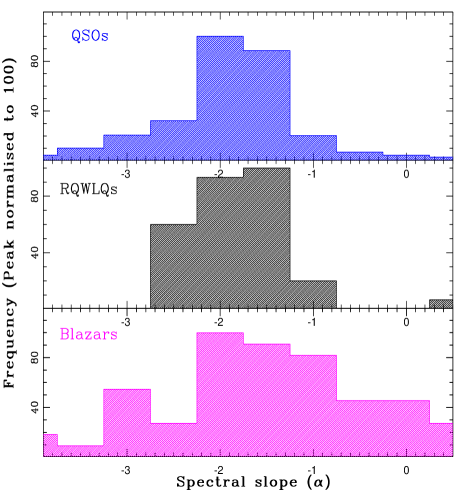
Figure 2: Spectral slope ($F_{\lambda}\propto\lambda^{\alpha}$) distribution for QSOs (upper panel), RQWLQs (middle panel) and blazars (lower panel).

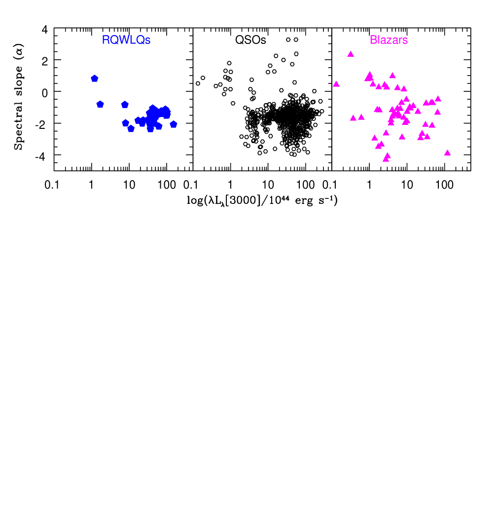
Figure 3: Spectral slope ($F_{\lambda}\propto\lambda^{\alpha}$) versus optical luminosity (in the rest-frame) for RQWLQs (left panel), QSOs (middle panel) and blazars (right panel).

The spectral slope distributions for the 3 AGN classes, viz. RQWLQs, QSOs and blazars, are shown in Fig. 2. The KS-test confirms that RQWLQs and blazars differ at a high level of significance (97.42$\%$) and so also the QSOs and blazars (99.97$\%$). In contrast, the difference between RQWLQs and QSOs has a much lower significance (61.17$\%$).

Here, we may point out the possibility of some bias creeping in while comparing the RQWLQs and blazars, on account of their occupying different luminosity ranges (since the redshifts of the RQWLQs are usually higher). To examine this, we show in Fig. 3 plots of the spectral slope versus optical luminosity ($\lambda$L_λ[3000Å]) for these three AGN classes. Since no significant correlation is seen between spectral slope and luminosity, any luminosity bias may not have a significant influence and the above inferred difference between the spectral slope distributions for RQWLQs and blazars is likely to be real (Fig. 2), suggesting a significant difference between their emission mechanisms and reinforcing the premise that RQWLQs are generally closer to QSOs in terms of emission mechanism.

4.2 Optical polarisation

The results of our polarimetry (Sect. 3) of the 6 bona-fide RQWLQs are summarized in Table 2. The first column of Table 2 gives the source name, while the next 3 columns give the percentage polarisation ($p$), polarisation angle (PA) and the date of observations. Two of the $6$ sources, namely J142505.59$+$035336.2 (on 2006.04.28) and J154515.77$+$003235.2 (in the sessions on 2006.04.25 and 2006.04.27) showed polarisation $p$ $>1\%$, albeit the excess was marginal. The highest observed polarisation in the present study is $1.59\pm 0.53\%$ for J154515.77$+$003235.2 on 2006.04.27. The two sources have also been covered in earlier polarimetric studies aimed at identifying BL Lacs among QSOs (Smith et al., 2007; Heidt & Nilsson, 2011). The polarisation values reported by these authors for J142505.59$+$035336.2 and J154515.77$+$003235.2, respectively, are $<$0.9%, $<$0.6%  (Smith et al., 2007) and $1.1\pm 0.6\%$, $<$5.6%  (Heidt & Nilsson, 2011). These are consistent with our measurements, suggesting a very mild polarisation variability for these AGN on year-like time scale. Both this and the observed polarisation of around $1\%$ for our RQWLQs is quite low compared to the average polarisation of around 7% found for classical BL Lacs (Heidt & Nilsson, 2011).

Once again, to check the possible role of bias arising from the difference in optical luminosity between our RQWLQs and the comparison sample of BL Lacs, we plot in Fig. 4 the polarisation against optical luminosity for the RQWLQs and BL Lacs. For our $6$ RQWLQs the polarisation measurement are taken from the present work, supplemented with the data from  Smith et al. (2007); Heidt & Nilsson (2011) for another $13$ RQWLQs which showed insignificant proper motion (e.g., see also Londish et al., 2002; Collinge et al., 2005). For the BL Lac comparison sample, we have taken the polarisation data from the work of  Heidt & Nilsson (2011). From Fig. 4, no correlation is evident between the percentage polarisation and optical luminosity. The linear Pearson correlation coefficients are $-0.58$ and $0.44$, respectively, for the RQWLQs and BL Lacs, which makes it unlikely that the inferred difference between their polarimetric properties could be an artefact of the luminosity difference between the two samples.

Table 2: The measured fractional polarisation ($p$) and polarisation angle (PA) for the 6 RQWLQs.

SDSS Name	$p$	P.A	Obs. Date
	(%)	(degree)	(yyyy.mm.dd)
(1)	(2)	(3)	(4)
J103607.52$+$015659.0	0.34$\pm$0.23	113	2006.04.26
J113413.48$+$001042.0	0.26$\pm$0.28	168	2006.04.27
J115909.61$-$024534.6	0.62$\pm$0.27	114	2006.04.26
J123437.64$-$012951.9	0.68$\pm$0.36	85	2006.04.27
J142505.59$+$035336.2	1.03$\pm$0.36	141	2006.04.28
J154515.77$+$003235.2	1.03$\pm$0.61	35	2006.04.25
	1.59$\pm$0.53	66	2006.04.27

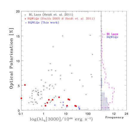
Figure 4: Optical luminosity versus optical polarisation ($p$) of RQWLQs from our sample (blue star), from Smith et al. (2007); Heidt & Nilsson (2011) (filled square) and the BL Lacs (open square) sample taken from Heidt & Nilsson (2011).

4.3 Long-term Variability Time Scale

Structure-function (SF) derived from a light curve is frequently used to infer the variability properties, such as the characteristics time-scales and any periodic behavior. Several definitions of SF have been used in the literature  (Graham et al., 2014). Here we adopt the definition of SF from  Hawkins (2002); Schmidt et al. (2010), and take an average over all the $N_{lc}$ light curves in a given sample (one light-curve for each object in the sample) as:

$$\tiny S(\tau)={}{}\vbox{\halign{\relax\begingroup\csname @IEEEeqnarraycolPREl\endcsname#\relax\relax\relax\relax\relax\relax\relax\relax\relax\relax\csname @IEEEeqnarraycolPOSTl\endcsname\relax\relax\relax\relax\relax\relax\relax\relax\relax\relax\endgroup&\relax\begingroup\csname @IEEEeqnarraycolPREs\endcsname#\relax\relax\relax\relax\relax\relax\relax\relax\relax\relax\csname @IEEEeqnarraycolPOSTs\endcsname\relax\relax\relax\relax\relax\relax\relax\relax\relax\relax\endgroup&\bgroup#\egroup\cr$\displaystyle\mbox{\vrule width=0.0pt,height=8.39996pt,depth=3.60004pt}\frac{1}{\sum_{k=1}^{N_{lc}}n^{k}(\tau)}\sum_{k=1}^{N_{lc}}\left(\sum_{i=1(i<j)}^{n^{k}(\tau)}\sqrt{\frac{\pi}{2}}[m^{k}(t_{j})-m^{k}(t_{i})]-\sqrt{\sigma_{i}^{2}+\sigma_{j}^{2}}\right)\mbox{\vrule width=0.0pt,height=8.39996pt,depth=3.60004pt}$\hfil&\vrule width=0.0pt,height=0.0pt,depth=0.0pt\hfil\crcr}}$$ (5)

where $m^{k}(t_{i})$ is the magnitude of the $k^{th}$ object at time $t_{i}$, and the sum runs over the $n^{k}$($\tau$) time intervals resulting from all possible combinations of $t_{j}-t_{i}=\tau$, with j$>$i in the light curve of the $k^{th}$ object in the sample. The $\sigma_{i}$ and $\sigma_{j}$ are the photometric errors on the measurements.

Our SF analysis (as per Eq. 5) makes use of the sample of the $40$ RQWLQs and the corresponding control samples of $800$ QSOs and $120$ blazars (see Sect. 4.1). The light curves of the RQWLQs, QSOs and blazars were taken from the CRTS archives, where for each night we have averaged the available V-band photometric data points (typically 3), in order to improve the SNR. The computed SFs for the 3 samples are shown in the Fig. 5. Clearly, the SF of RQWLQs is far better matched to that of the normal QSOs, as compared to the SF for blazars. This supports the premise that, as a class, RQWLQs are closer to normal QSOs in term of variability mechanism and are clearly different from blazars. The K-S test implies that the SFs for the RQWLQs and blazars differ at a high level of significance (99.99$\%$), which is also the case when the SFs of the QSOs and blazars are compared. In contrast, the SFs of RQWLQs and normal QSOs are practically indistinguishable.

Figure 5: Structure function (SF) for RQWLQs (open square), QSOs (filled circle) and blazars (blue stars). SFs for RQWLQs and the QSOs are similar, but its shape for blazars is very different (see text).

5 Discussion and Conclusions

Polarisation measurements have often been used to validate the BL Lac classification of AGN. For instance, as mentioned in Sect. 1, optical polarimetry of a large sample of 182 optically (spectroscopically) selected BL Lac candidates (both radio loud and radio quiet), by Heidt & Nilsson (2011), showed nearly half of them to be highly polarised ($p$$>$ 4%) and all these are radio loud. For another sample of similarly selected 42 BL Lac candidates, Smith et al. (2007) had earlier found that the sources with undetermined redshift were strongly polarised ($p$ going up to 23%), whereas at $z>1$ they found no source having $p>3$%. Again, their polarimetric search did not reveal a single good case of radio-quiet BL Lac.

In this study we have attempted to check if any of our 6 candidates, all of which are radio quiet, turns out to be a bona-fide BL Lac. The polarisation measurements for another $13$ of our objects having non-zero proper motions favoring a galactic classification will be presented elsewhere. The sensitive spectroscopic observations (though at lower spectral resolution), as reported here, have allowed us (i) to confirm the existing spectroscopic redshifts based on the SDSS spectra for 4 of our RQWLQs and (ii) to achieve a moderate improvement in redshift for the remaining two RQWLQs viz. J123437-012951, J142505+035336, without altering the inference on their extra-galactic nature consistent with their non-significant proper motions. Furthermore, with the SDSS spectra of the 40 RQWLQs (including the above 6 RQWLQs) have yielded the best-fit power-law slopes for their continuum spectra (Sect. 4.1; Fig. 1). This enabled a comparison with the spectral slope distribution we have determined for the two comparison samples, consisting of 800 QSOs and 120 blazars, using their SDSS spectra (Sect. 4.1). This statistical comparison, too, shows that in terms of optical spectral slope, RQWLQs are much more similar to QSOs than to blazars (e.g, see Fig. 2 and Sect. 4.1).

In the polarimetric data reported here for the $6$ bona-fide RQWLQs, only two sources, namely J142505.59$+$035336.2 and J154515.77$+$003235.2, observed in 3 sessions, were found to have polarisation $p$ in excess of $1\%$. However, the excess is marginal, with the highest value being $1.59\pm 0.53\%$, measured for J154515.77$+$003235.2 on 2006.04.27 (Table 2). Polarimetry of both these sources has earlier been reported by  Smith et al. (2007); Heidt & Nilsson (2011) and their results are fully consistent with the present measurements, suggesting that any polarisation variability must be modest.

We have argued that the present comparison of RQWLQs and BL Lacs is unlikely to suffer from the luminosity bias arising from a majority of our RQWLQs being located at higher-z and having systematically higher luminosities compared to the blazar comparison sample. This is because we do not find a significant dependence of $p$ on optical luminosity (Fig. 4), both for the blazar and RQWLQ samples. Therefore, the finding of much stronger optical polarisation for blazars, as compared to RQWLQs (for which $p$ is found here to be $<$ $\sim$ 1%), is likely to be an intrinsic difference. As mentioned above, polarisation for blazars is generally much higher. Among the 37 classical BL Lac objects observed by Jannuzi et al. (1994), $29$ were found to have $p>3\%$. The strong contrast again suggests that the mechanism responsible for the polarisation of the blazar emission plays a minor role in case of RQWLQs, although polarimetry of large samples of RQWLQs may still throw up some exceptions, which would be extremely interesting.

Lastly, we have also compared the long-term optical broad-band (V-band) variability of the 40 RQWLQs with that of the comparison samples of 800 normal QSOs and 120 blazars, taking the light curves from the archival CRTS database (Sect. 4.3). A comparison of their structure functions (Fig. 5) provides further support to the inference that, on the whole, the optical variability mechanism of RQWLQs is similar to that of QSOs and unlike that operating in blazars (which are generally more variable at all time-scales from $\sim$1 to $\sim$1000 days).

In summary, from the present study of RQWLQs, employing optical spectra, polarisation and temporal flux variation on medium to long time scale, it is evident that the mechanism of RQWLQs central engines is more similar to that operating in normal QSOs, as compared to blazars (where the emission is dominated by a Doppler boosted relativistic jet). A corollary of this would be that the abnormally weak emission lines in RQWLQs are probably better understood in terms of the model which invokes a less developed broad-line region with a low covering factor (Sect. 1). Such a low covering factor of the BLR in RQWLQs would have an additional consequence, namely an enhanced evaporation of dust in the torus, leading to a diminished infrared output. This would be in accord with the up-to 30-40$\%$ lower infrared emission detected by Diamond-Stanic et al. (2009) in their observations of two RQWLQs. A confirmation of this using a larger sample of RQWLQs would be very desirable.

References

- Abazajian et al. (2009) Abazajian K. N. et al., 2009, ApJS, 182, 543
- Antonucci (2012) Antonucci R., 2012, Astronomical and Astrophysical Transactions, 27, 557
- Begelman et al. (1984) Begelman M. C., Blandford R. D., Rees M. J., 1984, Reviews of Modern Physics, 56, 255
- Bolton et al. (2012) Bolton A. S. et al., 2012, AJ, 144, 144
- Buzzoni et al. (1984) Buzzoni B. et al., 1984, The Messenger, 38, 9
- Chand et al. (2014) Chand H., Kumar P., Gopal-Krishna, 2014, MNRAS, 441, 726
- Collinge et al. (2005) Collinge M. J. et al., 2005, AJ, 129, 2542
- Diamond-Stanic et al. (2009) Diamond-Stanic A. M. et al., 2009, ApJ, 699, 782
- Drake et al. (2009) Drake A. J. et al., 2009, ApJ, 696, 870
- Elitzur & Ho (2009) Elitzur M., Ho L. C., 2009, ApJ, 701, L91
- Gaia Collaboration et al. (2018) Gaia Collaboration, Brown A. G. A., Vallenari A., Prusti T., de Bruijne J. H. J., Babusiaux C., Bailer-Jones C. A. L., 2018, ArXiv e-prints
- Gaia Collaboration et al. (2016) Gaia Collaboration et al., 2016, A&A, 595, A1
- Gopal-Krishna et al. (2011) Gopal-Krishna, Goyal A., Joshi S., Karthick C., Sagar R., Wiita P. J., Anupama G. C., Sahu D. K., 2011, MNRAS, 416, 101
- Gopal-Krishna et al. (2013) Gopal-Krishna, Joshi R., Chand H., 2013, MNRAS, 430, 1302
- Gopal-Krishna et al. (2003) Gopal-Krishna, Stalin C. S., Sagar R., Wiita P. J., 2003, ApJ, 586, L25
- Goyal et al. (2012) Goyal A., Gopal-Krishna, Wiita P. J., Anupama G. C., Sahu D. K., Sagar R., Joshi S., 2012, A&A, 544, A37
- Graham et al. (2014) Graham M. J., Djorgovski S. G., Drake A. J., Mahabal A. A., Chang M., Stern D., Donalek C., Glikman E., 2014, MNRAS, 439, 703
- Hawkins (2002) Hawkins M. R. S., 2002, MNRAS, 329, 76
- Heidt & Nilsson (2011) Heidt J., Nilsson K., 2011, A&A, 529, A162
- Hewett & Wild (2010) Hewett P. C., Wild V., 2010, MNRAS, 405, 2302
- Hryniewicz et al. (2010) Hryniewicz K., Czerny B., Nikołajuk M., Kuraszkiewicz J., 2010, MNRAS, 404, 2028
- Jannuzi et al. (1994) Jannuzi B. T., Smith P. S., Elston R., 1994, ApJ, 428, 130
- Kellermann et al. (1989) Kellermann K. I., Sramek R., Schmidt M., Shaffer D. B., Green R., 1989, AJ, 98, 1195
- Kumar et al. (2016) Kumar P., Chand H., Gopal-Krishna, 2016, MNRAS, 461, 666
- Kumar et al. (2015) Kumar P., Gopal-Krishna, Chand H., 2015, MNRAS, 448, 1463
- Kumar et al. (2017) Kumar P., Gopal-Krishna, Stalin C. S., Chand H., Srianand R., Petitjean P., 2017, MNRAS, 471, 606
- Laor & Davis (2011) Laor A., Davis S. W., 2011, MNRAS, 417, 681
- Liu et al. (2015) Liu Y., Zhang J., Zhang S. N., 2015, A&A, 576, A3
- Liu & Zhang (2011) Liu Y., Zhang S. N., 2011, ApJ, 728, L44
- Londish et al. (2002) Londish D. et al., 2002, MNRAS, 334, 941
- Markwardt (2009) Markwardt C. B., 2009, in Astronomical Society of the Pacific Conference Series, Vol. 411, Astronomical Data Analysis Software and Systems XVIII, Bohlender D. A., Durand D., Dowler P., eds., p. 251
- Meusinger & Balafkan (2014) Meusinger H., Balafkan N., 2014, A&A, 568, A114
- Nicastro et al. (2003) Nicastro F., Martocchia A., Matt G., 2003, ApJ, 589, L13
- Nikołajuk & Walter (2012) Nikołajuk M., Walter R., 2012, MNRAS, 420, 2518
- Padovani & Giommi (1995) Padovani P., Giommi P., 1995, ApJ, 444, 567
- Plotkin et al. (2010a) Plotkin R. M. et al., 2010a, AJ, 139, 390
- Plotkin et al. (2010b) Plotkin R. M., Anderson S. F., Brandt W. N., Diamond-Stanic A. M., Fan X., MacLeod C. L., Schneider D. P., Shemmer O., 2010b, ApJ, 721, 562
- Sagar et al. (2004) Sagar R., Stalin C. S., Gopal-Krishna, Wiita P. J., 2004, MNRAS, 348, 176
- Schmidt et al. (2010) Schmidt K. B., Marshall P. J., Rix H.-W., Jester S., Hennawi J. F., Dobler G., 2010, ApJ, 714, 1194
- Smith et al. (2007) Smith P. S., Williams G. G., Schmidt G. D., Diamond-Stanic A. M., Means D. L., 2007, ApJ, 663, 118
- Stalin et al. (2004a) Stalin C. S., Gopal-Krishna, Sagar R., Wiita P. J., 2004a, MNRAS, 350, 175
- Stalin et al. (2004b) Stalin C. S., Gopal Krishna, Sagar R., Wiita P. J., 2004b, Journal of Astrophysics and Astronomy, 25, 1
- Stalin & Srianand (2005) Stalin C. S., Srianand R., 2005, MNRAS, 359, 1022
- Stocke et al. (1990) Stocke J. T., Morris S. L., Gioia I., Maccacaro T., Schild R. E., Wolter A., 1990, ApJ, 348, 141
- Stocke & Perrenod (1981) Stocke J. T., Perrenod S. C., 1981, ApJ, 245, 375
- Urry & Padovani (1995) Urry C. M., Padovani P., 1995, PASP, 107, 803
- York et al. (2000) York D. G. et al., 2000, AJ, 120, 1579