A new decision theoretic sampling plan for type-I and type-I hybrid censored samples from the exponential distribution

Abstract

The study proposes a new decision theoretic sampling plan (DSP) for Type-I and Type-I hybrid censored samples when the lifetimes of individual items are exponentially distributed with a scale parameter. The DSP is based on an estimator of the scale parameter which always exists, unlike the MLE which may not always exist. Using a quadratic loss function and a decision function based on the proposed estimator, a DSP is derived. To obtain the optimum DSP, a finite algorithm is used. Numerical results demonstrate that in terms of the Bayes risk, the optimum DSP is as good as the Bayesian sampling plan (BSP) proposed by Lin et al. (2002) and Liang and Yang (2013). The proposed DSP performs better than the sampling plan of Lam (1994) and Lin et al. (2008, 2008a) in terms of Bayes risks. The main advantage of the proposed DSP is that for higher degree polynomial and non-polynomial loss functions, it can be easily obtained as compared to the BSP.

Keywords and Phrases: Exponential distribution, Type-I and Type-I hybrid censoring, Decision theoretic sampling plan, Bayes risk, Bayesian sampling plan.
 
¹ Department of Mathematics and Statistics, Indian Institute of Technology Kanpur, India.
² Corresponding author e-mail: kundu@iitk.ac.in

1 Introduction

The sampling plan is an important instrument of any quality control experiment, which is used to test the quality of batch of items. A good sampling plan is important for manufacturers because a batch of items manufactured by them at the acceptable level of quality will have a good chance to be accepted by the plan. In the decision-theoretic approach, a sampling plan is determined by making an optimal decision on the basis of maximizing the return or minimizing the risk. So, for the economical point of view, it is more reasonable and realistic approach and therefore, it is widely employed by many statisticians. An extensive amount of work has been done along this line, see, for example, Hald (1967), Fertig and Mann (1974), Lam (1988), Lam (1994), Lin et al. (2002), Huang and Lin (2002, 2004), Chen et al. (2004), Lin et al. (2008, 2008a), Liang and Yang (2013),Tsai et al. (2014), and Liang et al. (2015).

In most of the life testing experiments, censoring is inevitable, i.e., the experiment terminates before all the experimental items fail. As a common practice, we put $n$ items on test and terminate the test when a preassigned $r$ number of items fail. This is known as the Type-II censoring, which ensures $r$ number of failures. But, in this case the experimental time would be unusually long for high quality items. To tackle this problem, the Type-I censoring scheme is used, in which we put $n$ items on test and terminate the test at a preassigned time $\tau$, no matter how many failures happen before the time $\tau$. Lam (1994) has provided a Bayesian sampling plan for a Type-I censoring scheme based on a suitable decision function and when the loss function is quadratic. Lin et al. (2002) has proved that Lam’s sampling plan is neither optimal nor Bayes and they have provided a Bayesian sampling plan in this case.

The hybrid censoring is more economical and logical because it combines the advantages of both types of censoring. In the Type-I hybrid censoring the experiment is terminated at the time $\tau^{*}=min\{X_{(r)},\tau\}$, where $\tau$ is a fixed time and $X_{(r)}$ is the time to the $r^{th}$ failure. In a Type-II hybrid censoring the experiment is terminated at the time $\tau^{*}=max\{X_{(r)},\tau\}$. Lin et al. (2008, 2008a) derived an optimal sampling plan for both hybrid censoring schemes using the Bayesian approach. Liang and Yang (2013) found the exact Bayes decision function and derived an optimum Bayesian sampling plan for the Type-I hybrid censoring based on a quadratic loss function. An extensive amount of literature is available on all the above sampling plans which are decision theoretic in nature and are based on the estimator of the mean lifetime of the exponential distribution.

In this paper, we develop a decision theoretic sampling plan (DSP) for Type-I and Type-I hybrid censored samples using a decision function which is based on a suitable estimator of $\lambda$ in place of the estimator of the mean lifetime $\displaystyle\theta=\frac{1}{\lambda}$. We consider the sampling plans $(n,\tau,\zeta)$ under the Type-I censoring and $(n,r,\tau,\zeta)$ under the Type-I hybrid censoring. Here, $n$, $r$ and $\tau$ are same as defined before, and $\zeta$ is the threshold point based on which we take a decision on the batch. Under such censoring schemes, the proposed estimator of $\lambda$ always exists unlike the MLE, which may not always exist. A loss function, which includes the sampling cost, the cost per unit time, the salvage value and the cost due to acceptance of the batch, is used to determine the DSP, by minimizing the Bayes risk. The optimum DSP is obtained for Type-I and Type-I hybrid censoring and numerically it has been observed that it is as good as the BSP in terms of the Bayes risk. It is also observed that the optimum DSP is better than the sampling plan of  Lam (1994) and Lin et al. (2008, 2008a). Theoretically it has been shown that the implementation of the DSP is easier compared to the BSP proposed by Lin et al. (2002) and Liang and Yang (2013), for higher degree polynomial and non-polynomial loss functions.

The rest of the paper is organized as follows. In Section 2, we present the decision function based on an estimator of $\lambda$. All necessary theoretical results for Type-I and Type-I hybrid censoring are provided in Sections 3 and 4, respectively. The DSP for higher degree polynomial and for non-polynomial loss functions are presented in Section 5. Numerical results are provided in Section 6. Finally, we conclude the paper in Section 7. All derivations are provided in the Appendix.

2 Problem Formulation and the Proposed Decision Rule

Suppose we are given a batch of items and we need to decide whether we want to accept or reject the batch. It is assumed that lifetimes of these items are mutually independent and follow an exponential distribution with the probability density function (PDF)

$$f(x)=\lambda e^{-\lambda x};\ \ \ \ x>0,\ \ \lambda>0.$$

To conduct a life testing experiment, $n$ identical items are sampled from the batch and placed on test without replacement with a suitable sampling scheme. Under Type-I and Type-I hybrid censoring schemes, let $\tau^{*}$ denote the duration of the experiment. Then $\tau^{*}=\tau$ in Type-I censoring and $\tau^{*}=min\{X_{(r)},\tau\}$ in Type-I hybrid censoring. Note that $\tau^{*}$ is fixed in Type-I censoring and random for Type-I hybrid censoring. Let $M$ be the number of failures observed before the fixed time $\tau$, i.e., $M=max\{i:X_{(i)}\leq\tau\}$. Hence, the observed sample is $(X_{(1)},X_{(2)},\ldots,X_{(M)})$ in Type-I censoring, and $(X_{(1)},X_{(2)},\ldots,X_{(r)})$ or $(X_{(1)},X_{(2)},\ldots,X_{(M)})$ in Type-I hybrid censoring. Based on the observed sample, we define the decision function as:

$$\delta(\textbf{x})=\begin{cases}d_{0}&\mbox{if}\ \widehat{\lambda}<\zeta,\\ d_{1}&\mbox{if}\ \widehat{\lambda}\geq\zeta,\end{cases}$$ (1)

where $\widehat{\lambda}$ is a suitable estimator of $\lambda$, $\zeta>0$ denotes the threshold point based on which we take a decision on the batch whether to accept (action $d_{0}$) or to reject it (action $d_{1}$).

Next, we consider a loss function which depends upon various costs. $C_{r}$ is the cost due to rejecting the batch; $C_{s}$ is the cost due to per item inspection; $C_{\tau}$ is the cost of per unit time and $g(\lambda)$ is the cost of accepting the batch. If an item does not fail, then the item can be reused with the salvage value $r_{s}$. Combining all these costs, the general form of the loss function (see Liang and Yang (2013), Liang et al. (2015)) is given as:

$$L(\delta(\textbf{x}),\lambda,n,r,\tau)=\begin{cases}nC_{s}-(n-M)r_{s}+\tau^{*}C_{\tau}+g(\lambda)&\mbox{if}\ \delta(\textbf{x})=d_{0},\\ nC_{s}-(n-M)r_{s}+\tau^{*}C_{\tau}+C_{r}&\mbox{if}\ \delta(\textbf{x})=d_{1}.\end{cases}$$ (2)

Clearly $C_{s}$, $C_{\tau}$, $C_{r}$ and $r_{s}$ are non-negative where $C_{s}>r_{s}$ and $g(\lambda)$ depends on the parameter $\lambda$. Smaller $\lambda$ indicates better quality of the item. Therefore, $g(\lambda)$ can take various forms which have to be positive and increasing with $\lambda$. A quadratic loss function has been widely used as an approximation of the true cost function when a batch is accepted (see Lam (1990), Lam (1994) and Lam and Choy (1995)). For a better approximation of the true loss function, higher degree polynomial loss function can be considered, i.e., cost of acceptance in the loss function (2) is considered as $g(\lambda)=a_{0}+a_{1}\lambda+\ldots+a_{k}\lambda^{k}$. It is notable that the true form of the loss function can vary because it includes costs that are difficult to recognize. To obtain the Bayes risk of the decision function (1) based on the loss function (2), it is assumed that $\lambda$ follows a gamma $(a,b)$ prior with the following PDF;

$$\pi(\lambda;a,b)=\frac{b^{a}}{\Gamma(a)}\lambda^{a-1}e^{-\lambda b},\ \ \ \ \lambda>0,\ \ a,b>0.$$ (3)

Next, we determine the optimum DSP $(n_{0},\tau_{0},\zeta_{0})$ for Type-I censoring and $(n_{0},r_{0},\tau_{0},\zeta_{0})$ for Type-I hybrid censoring such that it has the minimum Bayes risk among all possible sampling plans.

3 Bayes Risk and DSP under Type -I Censoring

Lin et al. (2002) derived the Bayes risk of the BSP for a quadratic loss function assuming $r_{s}=0$ and $g(\lambda)=a_{0}+a_{1}\lambda+a_{2}\lambda^{2}$, such that $a_{0}>0$, $a_{1}>0$ and $a_{2}>0$. This form of the loss function is widely used in the literature (see, for example, Hald (1967); Lam (1994); Lam and Choy (1995)). Likewise, we also derive the Bayes risk of the proposed DSP for a quadratic loss function with $r_{s}>0$, i.e., the loss function takes the following form;

$$L(\delta(\textbf{x}),\lambda,n,\tau)=\begin{cases}nC_{s}-(n-M)r_{s}+\tau C_{\tau}+a_{0}+a_{1}\lambda+a_{2}\lambda^{2}&\mbox{if}\quad\delta(\textbf{x})=d_{0},\\ nC_{s}-(n-M)r_{s}+\tau C_{\tau}+C_{r}&\mbox{if}\quad\delta(\textbf{x})=d_{1}.\end{cases}$$ (4)

To derive the Bayes risk for the decision function (1), we define a suitable estimator of $\lambda$ as follows:

$$\widehat{\lambda}=\begin{cases}\ \ \ \ \ \ 0\ \ \ \ \ \ \ \ \ \ \ \ \ \ \mbox{if}\ \ \ M=0\\ \ \ \ \ \ \ \widehat{\lambda}_{M}\ \ \ \ \ \ \ \ \ \ \ \mbox{if}\ \ \ M>0,\end{cases}$$

where $\widehat{\lambda}_{M}$ is the MLE of $\lambda$ given by,

$$\widehat{\lambda}_{M}=\frac{M}{\sum_{i=1}^{M}X_{(i)}+(n-M){\tau}}\ \ \ \ \mbox{if}\ \ \ M>0.\\$$

Then the Bayes risk is,

$$r(n,\tau,\zeta) = E\big{\{}L(\delta(\textbf{x}),\lambda,n,\tau)\big{\}}$$

$$= E_{\lambda}E_{X/\lambda}\big{\{}L(\delta(\textbf{x}),\lambda,n,\tau)\big{\}}$$

$$= n(C_{s}-r_{s})+E(M)r_{s}+\tau C_{\tau}+a_{0}+a_{1}\mu_{1}+a_{2}\mu_{2}$$

$$\quad+E_{\lambda}\big{\{}(C_{r}-a_{0}-a_{1}\lambda-a_{2}\lambda^{2})P(\widehat{\lambda}\geq\zeta)\big{\}},$$

where $\displaystyle\mu_{i}=E(\lambda^{i})$ for $i=1,2$. Now to find an explicit form of the Bayes risk we need to compute $P(\widehat{\lambda}\geq\zeta)$. Note that the distribution function of $\widehat{\lambda}$ can be written as follows

$$P(\widehat{\lambda}\leq x) =P(M=0)P(\widehat{\lambda}\leq x|M=0)+P(M\geq 1)P(\widehat{\lambda}\leq x|M\geq 1)$$

$$=pS(x)+(1-p)H(x),$$ (5)

where $p=P(M=0)=e^{-n\lambda\tau}$ and

$$S(x)=P(\widehat{\lambda}\leq x|M=0)=\begin{cases}1&\mbox{if}\ \ \ x\geq 0,\\ 0&\mbox{if}\ \ \ otherwise,\end{cases}$$

$$H(x)=P(\widehat{\lambda}\leq x|M\geq 1)=\begin{cases}\int_{0}^{x}h(u)du&\mbox{if}\ \ \ \frac{1}{n\tau}<x<\infty,\\ 0&\mbox{if}\ \ \ otherwise,\end{cases}$$

where $h(u)$ is the PDF of the absolutely continuous part of the CDF of $\widehat{\lambda}$, and it is provided below.

Lemma 3.1.

The PDF $h(y)$ is given as

$$h(y)=\frac{1}{1-p}\sum_{m=1}^{n}\sum_{j=0}^{m}\binom{n}{m}\binom{m}{j}(-1)^{j}\frac{e^{-\lambda(n-m+j)\tau}}{y^{2}}\pi\left(\frac{1}{y}-\tau_{j,m};m,m\lambda\right)$$

for  $\displaystyle\frac{1}{n\tau}<y<\infty$,   $\displaystyle\tau_{j,m}=(n-m+j)\frac{\tau}{m}$,   and  $\pi(\cdot)$ is as defined in (3).

Proof.

For $M\geq 1$, The MLE of the mean lifetime $\theta$ is given by $\widehat{\theta}_{M}=\frac{1}{\widehat{\lambda}}$, whose PDF is obtained by Bartholomew (1963). Therefore, the PDF of $\widehat{\lambda}$, given $M\geq 1$, is obtained by taking the transformation $\widehat{\lambda}=\frac{1}{\widehat{\theta}_{M}}$, because $\widehat{\theta}_{M}>0$.  

Lemma 3.1 is used to compute $P(\widehat{\lambda}\geq\zeta)$ and then we used this probability to derive an explicit expression of the Bayes risk of the DSP. The following theorem provides the Bayes risk of the DSP for a quadratic loss function (4), for any sampling plan $(n,\tau,\zeta)$ .

Theorem 3.1.

The Bayes risk for the quadratic loss function (4) is given by,

$$r(n,\tau,\zeta) =n(C_{s}-r_{s})+E(M)r_{s}+\tau C_{\tau}+a_{0}+a_{1}\mu_{1}+a_{2}\mu_{2}$$

$$+\sum_{l=0}^{2}C_{l}\frac{b^{a}}{\Gamma(a)}\bigg{[}\frac{\Gamma{(a+l)}}{(b+n\tau)^{(a+l)}}\textit{I}_{(\zeta=0)}+\sum_{m=1}^{n}\sum_{j=0}^{m}(-1)^{j}\binom{n}{m}\binom{m}{j}\frac{\Gamma{(a+l)}}{(C_{j,m})^{a+l}}I_{S^{*}_{j,m}}(m,a+l)\bigg{]}.$$

Proof.

See Appendix.  

Since the expression of the Bayes risk $r(n,\tau,\zeta)$ of the DSP is quite complicated, therefore, the optimal values of $n$, $\tau$ and $\zeta$ cannot be computed analytically. Lam (1994) has given a discretization method to find an optimal sampling plan. Here we use a similar approach to obtain optimal values of $n$, $\tau$ and $\zeta$, which minimizes the Bayes risk among all sampling plans.
Algorithm for finding the optimum DSP:

1. Fix $n$ and $\tau$; minimize $r(n,\tau,\zeta)$ with respect to $\zeta$ using a grid search method and denote the minimum Bayes risk by $r(n,\tau,\zeta_{0}(n,\tau))$.

2. For fixed $n$, minimize $r(n,\tau,\zeta_{0}(n,\tau))$ with respect to $\tau$ using a grid search method and denote the minimum Bayes risk by $r(n,\tau_{0}(n),\zeta_{0}(n,\tau_{0}(n)))$.

3. Choose the sample size $n_{0}$ such that

   $$r(n_{0},\tau_{0}(n_{0}),\zeta_{0}(n_{0},\tau_{0}(n_{0})))\leq r(n,\tau_{0}(n),\zeta_{0}(n,\tau_{0}(n)))\ \ \forall\ \ \ n\geq 0.$$

We denote the optimum DSP by $(n_{0},\tau_{0},\zeta_{0})$ and the corresponding Bayes risk by $r(n_{0},\tau_{0},\zeta_{0})$. It is observed that the optimum DSP is unique, see Section 6. The next theorem proves that the proposed algorithm is finite , i.e., we can find an optimum DSP in a finite number of search steps.

Theorem 3.2.

Assuming $0<\zeta\leq\zeta^{*}$, let us denote $r(n,\tau,\zeta^{\prime})=min_{0<\zeta\leq\zeta^{*}}r(n,\tau,\zeta)$ for some fixed $n\ (\geq 1)$ and $\tau$. Let $n_{0}$ and $\tau_{0}$ be the optimal sample size and censoring time, respectively . Then,

$$n_{0}\leq\min\bigg{\{}\frac{C_{r}}{C_{s}-r_{s}},\frac{a_{0}+a_{1}\mu_{1}+\ldots+a_{k}\mu_{k}}{C_{s}-r_{s}},\frac{r(n,\tau,\zeta^{\prime})}{C_{s}-r_{s}}\bigg{\}},$$

$$\tau_{0}\leq\min\bigg{\{}\frac{C_{r}}{C_{\tau}},\frac{a_{0}+a_{1}\mu_{1}+\ldots+a_{k}\mu_{k}}{C_{\tau}},\frac{r(n,\tau,\zeta^{\prime})}{C_{\tau}}\bigg{\}}.$$

Proof.

See Appendix.  

4 Bayes Risk and DSP under Type-I Hybrid Censoring

For the Type-I hybrid censored sample, Liang and Yang (2013) derived the Bayes risk of the BSP for a quadratic loss function assuming $g(\lambda)=a_{0}+a_{1}\lambda+a_{2}\lambda^{2}$, such that $a_{0}>0$, $a_{1}>0$ and $a_{2}>0$. Chen et al. (2004) also used the same form of the loss function to derive acceptance sampling plans for Type-I hybrid censoring. Similarly, we also derive the Bayes risk of the DSP for a quadratic loss function as follows:

$$L(\delta(\textbf{x}),\lambda,n,\tau)=\begin{cases}nC_{s}-(n-M)r_{s}+\tau^{*}C_{\tau}+a_{0}+a_{1}\lambda+a_{2}\lambda^{2}&\mbox{if}\quad\delta(\textbf{x})=d_{0},\\ nC_{s}-(n-M)r_{s}+\tau^{*}C_{\tau}+C_{r}&\mbox{if}\quad\delta(\textbf{x})=d_{1}.\end{cases}$$ (6)

To derive the Bayes risk for the decision function (1) we define a suitable estimator of $\lambda$ under Type-I hybrid censoring as:

$$\widehat{\lambda}=\begin{cases}0\ \ \ \ \ \ \ \ \ \ \ \ \ \ \mbox{if}\ \ \ M=0\\ \widehat{\lambda}_{M}\ \ \ \ \ \ \ \ \ \ \ \mbox{if}\ \ \ M>0,\end{cases}$$

where $\widehat{\lambda}_{M}$ is the MLE of $\lambda$ given by,

$$\widehat{\lambda}_{M}=\begin{cases}\frac{M}{\sum_{i=1}^{M}X_{(i)}+(n-M){\tau}}\ \ \ \ \ \mbox{if}\ \ \ M=1,2\ldots r-1,\\ \frac{r}{\sum_{i=1}^{r}X_{(i)}+(n-r){X_{(r)}}}\ \ \ \mbox{if}\ \ \ M=r.\end{cases}$$

Then the Bayes risk is,

$$r(n,r,\tau,\zeta) = E\big{\{}L(\delta(\textbf{x}),\lambda,n,\tau)\big{\}}$$

$$= E_{\lambda}E_{X/\lambda}\big{\{}L(\delta(\textbf{x}),\lambda,n,\tau)\big{\}}$$

$$= n(C_{s}-r_{s})+E(M)r_{s}+E(\tau^{*})C_{\tau}+a_{0}+a_{1}\mu_{1}+a_{2}\mu_{2}$$

$$\quad+E_{\lambda}\big{\{}(C_{r}-a_{0}-a_{1}\lambda-a_{2}\lambda^{2})P(\widehat{\lambda}\geq\zeta)\big{\}},$$

where $\displaystyle\mu_{i}=E(\lambda^{i})$ for $i=1,2$. In order to derive an explicit expression of the Bayes risk of the DSP $(n,r,\tau,\zeta)$, we need to compute $P(\widehat{\lambda}\geq\zeta)$. The distribution of $\widehat{\lambda}$ can be written in a similar form as in (3), and the corresponding $h(u)$ is given below.

Lemma 4.1.

The PDF $h(y)$ is given by

$$h(y)=\frac{1}{1-p}\Bigg{[}\sum_{m=1}^{r-1}\sum_{j=0}^{m}A_{j,m} \frac{1}{y^{2}}\pi\left(\frac{1}{y}-\tau_{j,m};m,m\lambda\right)+\frac{1}{y^{2}}\pi\left(\frac{1}{y};r,r\lambda\right)$$

$$+r\binom{n}{r}\sum_{k=1}^{r}\binom{r-1}{k-1}(-1)^{k}\frac{e^{-\lambda(n-r+k)\tau}}{y^{2}(n-r+k)}\pi\left(\frac{1}{y}-\tau_{k,r};r,r\lambda\right)\Bigg{]}$$

for $\displaystyle\frac{1}{n\tau}<y<\infty$,   $\displaystyle\tau_{j,m}=(n-m+j)\frac{\tau}{m}$,  $\displaystyle A_{j,m}=\binom{n}{m}\binom{m}{j}(-1)^{j}e^{-\lambda(n-m+j)\tau}$ and $\pi(\cdot)$ as defined in (3).

Proof.

For $M\geq 1$, The MLE of the mean lifetime $\theta$ is given by $\widehat{\theta}_{M}=\frac{1}{\widehat{\lambda}}$, whose PDF is obtained by Childs et al. (2003). Hence, the PDF of $\widehat{\lambda}$ for $M\geq 1$ can be easily obtained.  

Theorem 4.1.

The Bayes risk using the quadratic loss function (6) is given by

$$r(n,r,\tau,\zeta) = n(C_{s}-r_{s})+E(M)r_{s}+E(\tau^{*})C_{\tau}+a_{0}+a_{1}\mu_{1}+a_{2}\mu_{2}$$

$$\quad+\sum_{l=0}^{2}C_{l}\frac{b^{a}}{\Gamma(a)}\bigg{\{}\frac{\Gamma{(a+l)}}{(b+n\tau)^{(a+l)}}\textit{I}_{(\zeta=0)}+\sum_{m=1}^{n}\sum_{j=0}^{m}\binom{n}{m}\binom{m}{j}(-1)^{j}R_{l,j,m}+R_{l,r-n,r}$$

$$\hskip 71.13188pt+\sum_{k=1}^{r}\binom{n}{r}\binom{r-1}{k-1}(-1)^{k}\frac{r}{(n-r+k)}R_{l,k,r}\bigg{\}},$$

Proof.

See Appendix.  

As in the case of Type-I censoring, the expression of the Bayes risk $r(n,r,\tau,\zeta)$ of the DSP is also quite complicated, and optimal values of $n$, $r$, $\tau$ and $\zeta$ cannot be computed analytically. In the following steps, an alternative algorithm (see Lam (1994)) is considered to obtain optimal values of $n$, $r$, $\tau$ and $\zeta$ which minimize the Bayes risk among all sampling plans.

Algorithm for finding optimum DSP:
To find the optimal values of $n$, $r$, $\tau$ and $\zeta$ based on the Bayes risk, a simple algorithm is described in the following steps:

1. Fix $n$, $r$ and $\tau$; minimize $r(n,r,\tau,\zeta)$ with respect to $\zeta$ using a grid search method and denote the minimum Bayes risk by $r(n,r,\tau,\zeta_{0}(n,r,\tau))$.

2. For fixed $n$ and $r$, minimize $r(n,r,\tau,\xi_{0}(n,r,\tau))$ with respect to $\tau$ using a grid search method and denote the minimum Bayes risk by $r(n,r,\tau_{0}(n,r),\zeta(n,r,\tau_{0}(n,r)))$.

3. For fixed $n$, choose $r\leq n$ for which $r(n,r,\tau_{0}(n,r),\zeta(n,r,\tau_{0}(n,r)))$ is minimum and denote it by $r(n,r_{0}(n),\tau_{0}(n,r_{0}(n)),\zeta(n,r_{0}(n_{0}),\tau_{0}(n,r_{0}(n))))$.

4. Choose the sample size $n_{0}$ such that

   $$r(n_{0},r_{0}(n_{0}),\tau_{0}(n_{0},r_{0}(n_{0})), \zeta_{0}(n_{0},r_{0}(n_{0}),\tau_{0}(n_{0},r_{0}(n_{0}))))$$

   $$\leq r(n,r_{0}(n),\tau_{0}(n,r_{0}(n)),\zeta_{0}(n,r_{0}(n),\tau_{0}(n,r_{0}(n))))\ \ \forall\ \ \ n\geq 0.$$

We denote the optimum DSP by $(n_{0},r_{0},\tau_{0},\zeta_{0})$ and the minimum Bayes risk by $r(n_{0},r_{0},\tau_{0},\zeta_{0})$. In this case it is also observed that the optimum DSP is unique, see in Section 6.

It is difficult to find the optimal $\tau_{0}$ analytically because the Bayes risk expression is complicated. Tsai et al. (2014) suggested a numerical approach to choose a suitable range of $\tau$, say $[0,\tau_{\alpha}]$ where $\tau_{\alpha}$ is such that $P(0<X<\tau_{\alpha})=1-\alpha$ and $\alpha$ is a preassigned number satisfying $0<\alpha<1$. The choice of $\alpha$ depends on the prescribed precision. The higher the precision required, the smaller the value of $\alpha$ should be. They suggested the value of $\alpha=0.01$. The next theorem establishes that the proposed algorithm stops in a finite number of steps.

Theorem 4.2.

Assuming $0<\zeta\leq\zeta^{*}$, let us denote $r(n,r,\tau,\zeta^{\prime})=min_{0<\zeta\leq\zeta^{*}}r(n,r,\tau,\zeta)$ for some fixed $n\ (\geq 1)$ and $\tau$. Let $n_{0}$ be the optimal sample size. Then,

$$n_{0}\leq\min\bigg{\{}\frac{C_{r}}{C_{s}-r_{s}},\frac{a_{0}+a_{1}\mu_{1}+\ldots+a_{k}\mu_{k}}{C_{s}-r_{s}},\frac{r(n,r,\tau,\zeta^{\prime})}{C_{s}-r_{s}}\bigg{\}}$$

and $r_{0}\leq n_{0}$.

Proof.

Proof is similar to Theorem 3.2.  

5 Higher Degree Polynomial and Non Polynomial Loss Functions

In this section, we establish that for a higher degree polynomial loss function or for a non polynomial loss function, the implementation of the proposed DSP is much easier compared to the BSP.

5.1 Higher Degree Polynomial Loss Function

In Section 3 and 4 we consider the quadratic loss function as an approximation of the true loss function. In this section we consider a higher degree polynomial loss function, i.e., the cost of acceptance in the loss function (2) is $g(\lambda)=a_{0}+a_{1}\lambda+\ldots+a_{k}\lambda^{k}$. Based on the discussions in Section 4, it is observed that for $k\geq 5$, the implementation of the proposed DSP under the Type-I hybrid censoring is straightforward as compared to the BSP. The Bayes risk for the DSP under Type-I hybrid censoring for a $k^{th}$ degree polynomial loss function is given by

$$r(n,r,\tau,\zeta) = n(C_{s}-r_{s})+E(M)r_{s}+E(\tau^{*})C_{\tau}+a_{0}+a_{1}\mu_{1}+a_{2}\mu_{2}+\ldots+a_{k}\mu_{k}$$ (7)

$$\quad+\sum_{l=0}^{k}C_{l}\frac{b^{a}}{\Gamma(a)}\bigg{\{}\frac{\Gamma{(a+l)}}{(b+n\tau)^{(a+l)}}\textit{I}_{(\zeta=0)}+\sum_{m=1}^{n}\sum_{j=0}^{m}\binom{n}{m}\binom{m}{j}(-1)^{j}R_{l,j,m}+R_{l,r-n,r}$$

$$\hskip 71.13188pt+\sum_{k=1}^{r}\binom{n}{r}\binom{r-1}{k-1}(-1)^{k}\frac{r}{(n-r+k)}R_{l,k,r}\bigg{\}},$$

where $E(M)$ and $E(\tau^{*})$ are defined earlier. Thus, for any value of $k$, obtaining the Bayes risk is straightforward and the form of the decision function is same for any value of $k$.

Now in case of the BSP, the Bayes decision rule (see Liang and Yang (2013)) is given by

$$\delta_{B}(\textbf{x})=\begin{cases}1,&\mbox{if}\ \ \phi_{\pi}\big{(}m,z\big{)}\leq C_{r}\\ 0,&\ \ \ \ \ \ otherwise,\end{cases}$$

where, for Type-I censoring

$$z=\sum_{i=1}^{m}x_{i}+(n-m)\tau,$$

and for Type-I hybrid censoring

$$z=\begin{cases}\sum_{i=1}^{m}x_{i}+(n-m)\tau&\mbox{if}\ \ \ \ m=1,2\ldots r-1\\ \sum_{i=1}^{r}x_{i}+(n-r)x_{r}&\mbox{if}\ \ \ \ m=r,\\ \end{cases}$$

with

$$\phi_{\pi}\big{(}m,z\big{)}=\int_{0}^{\infty}g(\lambda)\pi\big{(}\lambda|m,z\big{)}d\lambda.$$

Since the prior distribution of $\lambda$ is gamma $(a,b)$, it is well known that the posterior distribution of $\lambda$ is also gamma, viz.,

$$\pi\big{(}\lambda|m,z\big{)}\sim\hbox{gamma}(m+a,z+b).$$

Now when $g(\lambda)=a_{0}+a_{1}\lambda+\ldots+a_{k}\lambda^{k}$ in (2) then,

$$\phi_{\pi}\big{(}m,z\big{)}=\int_{0}^{\infty}g(\lambda)\pi\big{(}\lambda|m,z\big{)}d\lambda=a_{0}+\sum_{j=1}^{k}a_{j}\frac{(m+a)\ldots(m+a+j-1)}{(z+b)^{j}}.$$

Thus, to find the closed form of the decision function we need to obtain the set

$$A=\{z;\ z\geq 0,\phi_{\pi}\big{(}m,z\big{)}\leq C_{r}\},$$

and to construct the set $A$, we need to obtain the set of $z\geq 0$, such that

$$h_{1}(z)=a_{0}+\sum_{j=1}^{k}a_{j}\frac{(m+a)\ldots(m+a+j-1)}{(z+b)^{j}}\leq C_{r},$$ (8)

which is equivalent to find $z\geq 0$, such that,

$$h_{2}(z) = (C_{r}-a_{0})\big{(}z+b\big{)}^{k}-\sum_{j=1}^{k}a_{j}(m+a)\ldots(m+a+j-1)\big{(}z+b\big{)}^{k-j}\geq 0.$$ (9)

It can be easily shown that if $D_{n}(m)$ is the only real root or $D_{n}(m)$ is the maximum real root of $h_{2}(z)=0$ then the Bayes decision function will take the following form.

$$\delta_{B}(\textbf{x})=\begin{cases}1,&\mbox{if}\ \ z\geq a(n,r,\tau,m)\\ 0,&\ \ \ \ \ \ otherwise,\end{cases}$$ (10)

where  $a(n,r,\tau,0)=0\vee(D_{n}(0)-b)$ and $a(n,r,\tau,m)=0\vee(D_{n}(m)-b)\wedge n\tau\ \ \forall\ 1\leq m\leq r$. However, it is not straightforward to find the real root when $k\geq 5$. It is well known that there is no algebraic solution to polynomial equations of degree five or higher (see chapter 5, Herstein (1975)). So the BSP cannot be obtained for fifth or higher degree polynomial loss function analytically. Even, finding the optimal sampling plan numerically becomes very difficult.

5.2 Non-Polynomial Loss Function

We have already discussed in Section 2 that the loss due to accepting the batch $g(\lambda)$ can vary and the true form of the loss function is likely to be unknown. When we have a non-polynomial loss function, we show that implementation of the proposed DSP is quite easy and the associated Bayes risk is computed without any additional effort as compared to the BSP. To illustrate this, we use the following non polynomial loss function:

$$L(\delta(\textbf{x}),\lambda,n,r,\tau)=\begin{cases}nC_{s}-(n-M)r_{s}+\tau^{*}C_{\tau}+a_{0}+a_{1}\lambda+a_{2}\lambda^{5/2}&\mbox{if}\ \delta(\textbf{x})=d_{0},\\ nC_{s}-(n-M)r_{s}+\tau^{*}C_{\tau}+C_{r}&\mbox{if}\ \delta(\textbf{x})=d_{1},\end{cases}$$ (11)

where $g(\lambda)=a_{0}+a_{1}\lambda+a_{2}\lambda^{5/2}$ is an increasing function in $\lambda$. Here we consider only the Type-I hybrid censoring case. The Bayes risk of the DSP for the Type-I hybrid censoring is as follows:

$$r(n,r,\tau,\zeta) = n(C_{s}-r_{s})+E(M)r_{s}+E(\tau^{*})C_{\tau}+a_{0}+a_{1}\mu_{1}+a_{2}\frac{\Gamma{(a+\frac{5}{2}})}{\Gamma{(a)}b^{\frac{5}{2}}}$$

$$\quad+\sum_{l=0}^{2}C_{l}\frac{b^{a}}{\Gamma(a)}\bigg{\{}\frac{\Gamma{(a+p_{l})}}{(b+n\tau)^{(a+p_{l})}}\textit{I}_{(\zeta=0)}+\sum_{m=1}^{n}\sum_{j=0}^{m}\binom{n}{m}\binom{m}{j}(-1)^{j}R_{p_{l},j,m}$$

$$\hskip 71.13188pt+R_{p_{l},r-n,r}+\sum_{k=1}^{r}\binom{n}{r}\binom{r-1}{k-1}(-1)^{k}\frac{r}{(n-r+k)}R_{p_{l},k,r}\bigg{\}},$$

where $E(M)$ and $E(\tau^{*})$ are defined earlier and

$$p_{l}=\begin{cases}0,&\mbox{if}\ \ \ \ l=0\\ 1,&\mbox{if}\ \ \ \ l=1\\ \frac{5}{2},&\mbox{if}\ \ \ \ l=2.\end{cases}$$

To express the Bayes decision function of the BSP (see Liang and Yang (2013)) in a simpler form for the non-polynomial loss function $g(\lambda)=a_{0}+a_{1}\lambda+a_{2}\lambda^{5/2}$, we have to consider,

$$\phi_{\pi}\big{(}m,y(n,r,\tau,m)\big{)} =\int_{0}^{\infty}g(\lambda)\pi\big{(}\lambda|m,y(n,r,\tau,m)\big{)}d\lambda$$

$$=a_{0}+\frac{a_{1}(m+a)}{(y(n,r,\tau,m)+b)}+\frac{a_{2}\Gamma(m+a+\frac{5}{2})}{\Gamma(m+a)(y(n,r,\tau,m)+b)^{\frac{5}{2}}}.$$

So to find a closed form of the decision function we need to obtain the set

$$A=\{x;\ x\geq 0,\phi_{\pi}\big{(}m,x\big{)}\leq C_{r}\}.$$

Note that to construct the set $A$, we need to obtain the set of $x\geq 0$ such that

$$h_{1}(x)=a_{0}+\frac{a_{1}(m+a)}{(x+b)}+\frac{a_{2}\Gamma(m+a+\frac{5}{2})}{\Gamma(m+a)(x+b)^{\frac{5}{2}}}\leq C_{r},$$

and this is equivalent to find $x\geq 0$ such that

$$h_{2}(x)=(C_{r}-a_{0})\Gamma(m+a)\big{(}x+b\big{)}^{\frac{5}{2}}-a_{1}(m+a)\Gamma(m+a)\big{(}x+b\big{)}^{\frac{3}{2}}-a_{2}\Gamma(m+a+\frac{5}{2})\geq 0.$$

It is obvious that we cannot obtain a closed form solution of the non polynomial equation $h_{2}(x)=0$. So in case of a general non-polynomial loss function, we cannot construct a closed form of the Bayes decision function and obtain the explicit expression of Bayes risk. But since our decision function does not depend on the form of the loss function, this difficulty does not arise in case of the proposed DSP.

6 Numerical Results and Discussion

To obtain the numerical results, we consider the algorithms proposed in Sections 3 and 4 for Type-I and Type-I hybrid censoring, respectively. Let us assume that $n_{1}^{*}$ and $n_{2}^{*}$ from Theorem 3.2 and 4.2 denote the upper bound of $n_{0}$ under Type-I censoring and Type-I hybrid censoring, respectively. Then, for Type-I censoring

$$0\leq n_{0}\leq n_{1}^{*}\ \ \ and\ \ \ 0\leq\tau_{0}\leq\tau^{\prime},$$

and for Type-I hybrid censoring

$$0\leq n_{0}\leq n_{2}^{*}\ \ \ and\ \ \ 0\leq\tau_{0}\leq\tau_{\alpha},$$

where $\tau^{\prime}$ and $\tau_{\alpha}$ are upper bounds of $\tau$ under Type-I and Type-I hybrid censoring. For fixed $n$ and $\tau$ in Type-I censoring and for fixed $n$, $r\ (\leq n)$ and $\tau$ in Type-I hybrid censoring, we minimize the Bayes risk with respect to $\zeta$ using a grid search method where the grid size of $\zeta$ is taken as $0.0125$. Then, we minimize with respect to $\tau$ where grid size of $\tau$ is taken as $0.0125$. Finally, we choose the value of $n$ in Type-I censoring and the value of $n$ and $r\ (\leq n)$ in Type-I hybrid censoring for which the Bayes risk is minimum.

6.1 Comparison with Lam (1994), Lin et al. (2010) and BSP sampling plans

In this section, we focus on comparing the optimum DSP with Lam (1994), Lin et al. (2010) and BSP sampling plans. For Type-I censoring, comparison with Lam (1994) and Lin et al. (2010) sampling plans the values of coefficients $\ a_{0}=2,\ a_{1}=2,\ a_{2}=2,\ C_{s}=0.5,\ C_{\tau}=0$, $r_{s}=0$ and $C_{r}=30$ are used. In Table 1 only hyper-parameters $a$ and $b$ are varying and others are kept fixed.

Table 1: Numerical comparison with Lam (1994) and Lin et al. (2010) sampling plans for different values of $a$ and $b.$

Scheme	$a$	$b$	$r(n_{0},\tau_{0},\zeta_{0}(\xi_{0}))$	$n_{0}$	$\tau_{0}$	$\zeta_{0}(\xi_{0})$	$a$	$b$	$r(n_{0},\tau_{0},\zeta_{0})$	$n_{0}$	$\tau_{0}$	$\zeta_{0}(\xi_{0})$
DSP	2.5	0.8	24.8419	4	1.3125	3.0475	1.5	0.8	16.5825	3	0.7000	4.2862
LAM			24.9367	3	0.7077	0.3539			16.6233	3	0.5262	0.2631
Lin et al.(2010)			24.9893	4	0.6808	0.3404			16.7533	3	0.5262	0.2631
DSP	2.5	1.0	21.7081	4	1.1125	3.5950	2.0	0.8	21.1398	4	1.1625	3.4500
LAM			21.7640	3	0.5483	0.2742			21.2153	3	0.6051	0.3026
Lin et al.(2010)			21.8515	4	0.5819	0.2910			21.2875	4	0.6051	0.3026
DSP	3.0	0.8	27.5581	3	1.1625	2.5875	2.5	0.6	27.7267	3	1.2125	2.4863
LAM			27.6136	3	0.8170	0.4085			27.7834	3	0.8537	0.4268
Lin et al.(2010)			27.6521	3	0.8170	0.4085			29.8193	3	0.8537	0.4268
DSP	3.5	0.8	29.2789	2	1.0125	1.9875	10.0	3.0	29.5166	2	0.8000	2.5187
LAM			29.2789	2	1.0037	0.5019			29.5166	2	0.7928	0.3964
Lin et al.(2010)			29.3642	2	1.0037	0.5019			29.5959	2	0.8194	0.4097

From Table 1 it is clear that Bayes risk of the optimum DSP is less then or equal to the Bayes risk of Lam (1994) and Lin et al. (2010) sampling plans.

For Type-I censoring to compare with the BSP proposed by Lin et al. (2002) we use set of coefficient $a_{0}=2,a_{1}=2,a_{2}=2,C_{s}=0.5,C_{\tau}=0.5,C_{r}=30$, the prior parameters $a=2.5,b=0.8$ and assume $\zeta^{*}=6$. We obtain the minimum Bayes risk and decision theoretic sampling plan (DSP) for the proposed method and the Bayes risk of the BSP by varying $a$, $b$, $C_{s}$, $C_{\tau}$ and $C_{r}$ one at a time and keeping other fixed. The results are presented in Table 2.

Table 2: Numerical Comparison between DSP and BSP for Type-I censoring and Hybrid Type-I censoring.

	Type-I censoring							Hybrid Type-I censoring
$a$	$b$	BSP	DSP				$a$	$b$	BSP	DSP
		$r(n_{B},\tau_{B},\delta_{B})$	$r(n_{0},\tau_{0},\zeta_{0})$	$n_{0}$	$\tau_{0}$	$\zeta_{0}$			$r(n_{B},\tau_{B},\delta_{B})$	$r(n_{0},r_{0},\tau_{0},\zeta_{0})$	$n_{0}$	$r_{0}$	$\tau_{0}$	$\zeta_{0}$
2.5	0.8	25.2777	25.2777	3	0.7250	2.9750	2.5	0.8	26.0319	26.0338	6	3	0.2000	2.9750
2.5	1.0	22.0361	22.0361	3	0.5625	3.7250	2.5	1.0	22.6430	22.6437	5	3	0.1875	3.7200
3.5	0.8	29.7131	29.7131	2	0.8125	1.9875	3.0	0.8	28.7885	28.7889	4	2	0.2375	2.3445
$C_{s}$							$C_{s}$
0.50		25.2777	25.2777	3	0.7250	2.9750	0.30		24.3326	24.3341	10	4	0.1500	3.0500
1.00		26.5396	26.5396	2	0.5875	2.8625	0.50		26.0319	26.0338	6	3	0.2000	2.9750
2.00		27.9542	27.9542	1	0.3750	2.6750	0.70		26.9106	26.9114	3	2	0.2750	2.8625
$C_{\tau}$							$C_{\tau}$
0.50		25.2777	25.2777	3	0.7250	2.9750	0		24.6354	24.6754	4	4	0.8750	3.0500
1.00		25.6238	25.6238	3	0.6625	2.9750	8		26.4662	26.4672	7	3	0.1625	2.9750
2.00		26.1439	26.1439	4	0.3875	2.9750	16		27.2513	27.2513	7	2	0.1000	1.9625
$C_{r}$							$C_{r}$
20		19.3293	19.3293	2	0.8750	1.7750	25		23.3583	23.3581	4	2	0.2375	2.2875
30		25.2777	25.2777	3	0.7250	2.9750	30		26.0319	26.0338	6	3	0.2000	2.9750
50		32.2092	32.2092	5	0.5625	5.0500	40		30.0072	30.0069	7	4	0.1750	4.0750

Similarly for the Type-I hybrid censoring, comparison is made between the BSP proposed by Liang and Yang (2013) and the proposed DSP by taking set of coefficients $a_{0}=2,a_{1}=2,a_{2}=2,C_{s}=0.5,r_{s}=0.3,C_{\tau}=5.0,C_{r}=30$, the hyper parameters $a=2.5,b=0.8$ and assume $\zeta^{*}=6$. The Bayes risk of the BSP involves a complicated integral, and it has been approximated by Monte Carlo simulation. So the Bayes risk here is an approximation of the exact Bayes risk of the BSP.

Further, when the Bayes risk has a unique minimum, the proposed algorithm gives us the optimum DSP without any additional computational effort. Since the Bayes risk expression is quite complicated, it is not easy to prove theoretically that the function has a unique minimum. So we study graphical behavior of the Bayes risk by providing its contour plots with respect to $\tau$ (on x-axis) and $\zeta$ (on y- axis) with hyper parameter $a=2.5$, $b=0.8$ and set of coefficients mentioned above for Type-I and Type-I hybrid censoring.

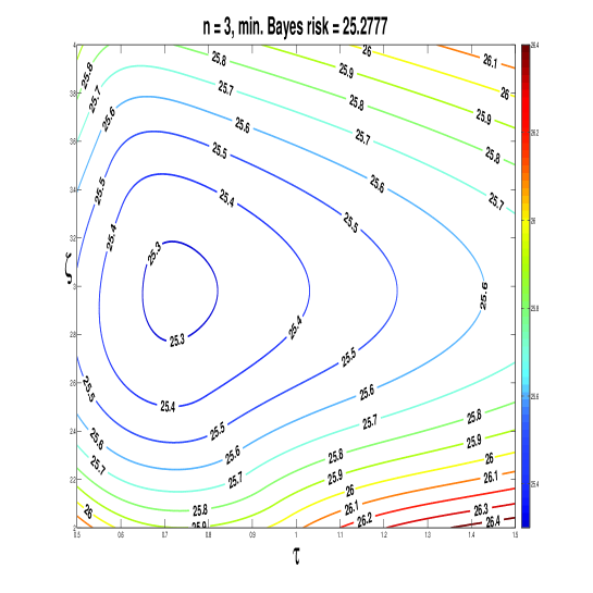
(a)

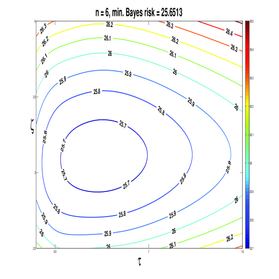
(b)

Figure 1: Contour plot of Bayes risk with set of coefficient $a_{0}=2,a_{1}=2,a_{2}=2,C_{s}=0.5,r_{s}=0,C_{\tau}=0.5,C_{r}=30$ and $a=2.5,b=0.8$ for Type-I censoring.

In Type-I censoring, the Bayes risk is a function of three parameters which are $n$, $\tau$ and $\zeta$, among which one is discrete and two are continuous. Since $n$ takes discrete values and from Theorem 3.2 we know that optimal value of $n$ is bounded above, so for different values of $n$, we provide the contour plot of Bayes risk with respect to $\tau$ and $\zeta$ in Figure 1. It is clear from contour plot that the Bayes risk has a unique minimum with respect to $\tau$ and $\zeta$. We also observe that the Bayes risk first decreases then increases as $n$ increases.

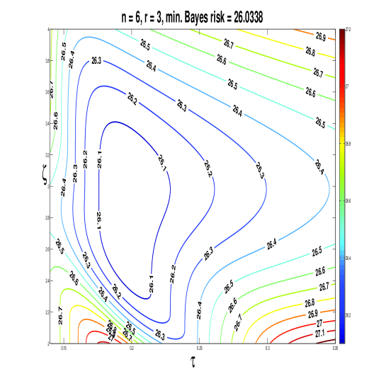
(a)

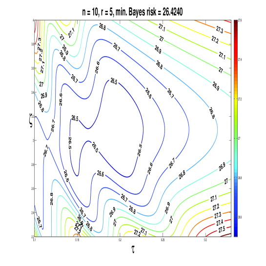
(b)

Figure 2: Contour plot of Bayes risk with set of coefficient $a_{0}=2,a_{1}=2,a_{2}=2,C_{s}=0.5,r_{s}=0.3,C_{\tau}=5.0,C_{r}=30$ and $a=2.5,b=0.8$ for Type-I hybrid censoring.

Similarly for Type-I hybrid censoring, Bayes risk is a function of four parameters $n$, $r$, $\tau$, and $\zeta$ among which two are discrete and two continuous. Since optimal values of $n$ and $r$ are bounded above(see Theorem 4.2), so for different values of $n$ and $r$, we provide the contour plots of Bayes risk with respect to $\tau$ and $\zeta$ in Figure 2. In this case also Bayes risk has unique minimum and as $n$ increases Bayes risk first decreases then increases. The contour plot can also be used for predicting the range which includes the optimal values of $\tau$ and $\zeta$.

6.2 Numerical results for Higher degree polynomial and Non polynomial loss function

In Section 5 we have observed that for a higher degree polynomial and for a non polynomial loss function the DSP can be obtained without any additional effort as compared to the BSP. The numerical results for fifth degree polynomial and for non polynomial loss function are tabulated in Tables 3-24. Standard values of parameter, coefficients and costs are defined in every section where needed. In each table, only hyper parameters $a$ and $b$ or one coefficient or one cost can change and the others are kept fixed. It should be clear from the tables.

6.2.1 Fifth Degree Polynomial Loss Function

For Type-I hybrid censoring, we present the optimum DSP for fifth degree polynomial loss function, with the standard set of hyper parameter, coefficients and costs: $a=1.5,b=0.8,a_{0}=2,a_{1}=2,a_{2}=2,a_{3}=2,a_{4}=2,a_{5}=2,C_{r}=30,C_{s}=0.5,r_{s}=0.3,C_{\tau}=0.5,\zeta^{*}=6$. In Tables 3-8 the values of the different hyper parameters or coefficients or costs are given in column $1$ and $7$. The minimum Bayes risk $r(n_{0},r_{0},\tau_{0},\zeta_{0})$ and the corresponding optimal sampling plan $(n_{0},r_{0},\tau_{0},\zeta_{0})$ are given in columns $2-6$ and $8-12$.

Table 3: The minimum Bayes risk and optimum DSP for Type-I hybrid censoring as $a$ and $b$ varies

$a$	$b$	$r(n_{0},r_{0},\tau_{0},\zeta_{0})$	$n_{0}$	$r_{0}$	$\tau_{0}$	$\zeta_{0}$
0.2	0.2	12.1795	5	4	1.2625	0.9750
1.5	0.4	29.6469	2	2	2.9125	0.6250
1.5	0.8	26.2983	5	4	1.6375	0.9250
2.5	1.5	27.8324	5	4	1.6750	0.9250
3.0	1.5	29.9061	4	3	1.7000	0.7500

Table 4: The minimum Bayes risk and optimum DSP for Type-I hybrid censoring as $a_{0}$ or $a_{1}$ varies

$a_{0}$	$r(n_{0},r_{0},\tau_{0},\zeta_{0})$	$n_{0}$	$r_{0}$	$\tau_{0}$	$\zeta_{0}$	$a_{1}$	$r(n_{0},r_{0},\tau_{0},\zeta_{0})$	$n_{0}$	$r_{0}$	$\tau_{0}$	$\zeta_{0}$
0.5	25.8251	6	5	1.6625	1.0000	0.5	26.0091	6	5	1.6625	1.0000
1.0	25.9891	5	4	1.6250	0.9375	1.0	26.1080	5	4	1.6250	0.9375
1.5	26.1444	5	4	1.6375	0.9375	1.5	26.2038	5	4	1.6375	0.9375
2.0	26.2983	5	4	1.6375	0.9250	2.0	26.2983	5	4	1.6375	0.9250
2.5	26.4515	5	4	1.6500	0.9250	2.5	26.3919	5	4	1.6500	0.9250

Table 5: The minimum Bayes risk and optimum DSP for Type-I hybrid censoring as $a_{2}$ or $a_{3}$ varies

$a_{2}$	$r(n_{0},r_{0},\tau_{0},\zeta_{0})$	$n_{0}$	$r_{0}$	$\tau_{0}$	$\zeta_{0}$	$a_{3}$	$r(n_{0},r_{0},\tau_{0},\zeta_{0})$	$n_{0}$	$r_{0}$	$\tau_{0}$	$\zeta_{0}$
0.5	26.0403	6	5	1.6625	1.0125	0.5	25.9983	6	5	1.6250	1.0125
1.0	26.1284	5	4	1.6250	0.9375	1.0	26.1027	5	4	1.6125	0.9500
1.5	26.2141	5	4	1.6250	0.9375	1.5	26.2022	5	4	1.6250	0.9375
2.0	26.2983	5	4	1.6375	0.9250	2.0	26.2983	5	4	1.6375	0.9250
2.5	26.3810	5	4	1.6500	0.9250	2.5	26.3911	5	4	1.6500	0.9125

Table 6: The minimum Bayes risk and optimum DSP for Type-I hybrid censoring as $a_{4}$ or $a_{5}$ varies

$a_{4}$	$r(n_{0},r_{0},\tau_{0},\zeta_{0})$	$n_{0}$	$r_{0}$	$\tau_{0}$	$\zeta_{0}$	$a_{5}$	$r(n_{0},r_{0},\tau_{0},\zeta_{0})$	$n_{0}$	$r_{0}$	$\tau_{0}$	$\zeta_{0}$
0.5	25.8618	6	5	1.5875	1.0500	0.5	25.4497	5	4	1.4125	1.0750
1.0	26.0212	5	4	1.5750	0.9625	1.0	25.8046	5	4	1.5000	1.0125
1.5	26.1656	5	4	1.6125	0.9500	1.5	26.0771	5	4	1.5750	0.9625
2.0	26.2983	5	4	1.6375	0.9250	2.0	26.2983	5	4	1.6375	0.9250
2.5	26.4212	5	4	1.6750	0.9125	2.5	26.4838	5	4	1.7000	0.9000

Table 7: The minimum Bayes risk and optimum DSP for Type-I hybrid censoring as $C_{s}$ or $C_{\tau}$ varies

$C_{s}$	$r(n_{0},r_{0},\tau_{0},\zeta_{0})$	$n_{0}$	$r_{0}$	$\tau_{0}$	$\zeta_{0}$	$C_{\tau}$	$r(n_{0},r_{0},\tau_{0},\zeta_{0})$	$n_{0}$	$r_{0}$	$\tau_{0}$	$\zeta_{0}$
0.4	25.6655	7	5	1.2375	0.9875	0.2	25.9954	4	4	3.1375	0.9250
0.5	26.2983	5	4	1.6375	0.9250	0.5	26.2983	5	4	1.6375	0.9250
0.8	27.4684	3	3	2.8000	0.8375	0.8	26.5453	6	4	1.1375	0.9250
1.0	27.9656	2	2	2.5125	0.7125	1.2	26.8039	6	4	1.1125	0.9250
1.5	28.9099	1	1	2.0375	0.0125	1.5	26.9779	7	4	0.8625	0.9250

From Table 3 it is clear that as $a$ increases for fixed $b$ the minimum Bayes risk increases and as $b$ increases for fixed $a$ the minimum Bayes risk decreases. In Tables 4-6 we observed that as coefficients $a_{0},a_{1},a_{2},a_{3},a_{4}$ and $a_{5}$ increases the minimum Bayes risk increases. In Tables 7-8 if costs $C_{s},C_{\tau}$ and $C_{r}$ increases then the minimum Bayes risk increases and when the salvage value $r_{s}$ increases, the minimum Bayes risk decreases.

Table 8: The minimum Bayes risk and optimum DSP for Type-I hybrid censoring as $C_{r}$ or $r_{s}$ varies

$C_{r}$	$r(n_{0},r_{0},\tau_{0},\zeta_{0})$	$n_{0}$	$r_{0}$	$\tau_{0}$	$\zeta_{0}$	$r_{s}$	$r(n_{0},r_{0},\tau_{0},\zeta_{0})$	$n_{0}$	$r_{0}$	$\tau_{0}$	$\zeta_{0}$
25	22.7787	4	3	1.5750	0.7875	0.05	26.5544	4	4	3.0250	0.9250
35	29.6324	6	5	1.6375	1.0375	0.10	26.5352	4	4	3.0000	0.9250
50	38.8182	8	7	1.5375	1.2500	0.20	26.4478	5	4	1.6625	0.9250
65	47.1201	10	9	1.4500	1.4125	0.30	26.2983	5	4	1.6375	0.9250
85	57.2562	12	11	1.3750	1.5625	0.35	26.2220	6	4	1.1375	0.9250

For Type-I censoring, we present the optimum DSP for the fifth degree polynomial, with the following standard set of hyper parameters, coefficients and costs: $a=1.5,b=0.8,a_{0}=2,a_{1}=2,a_{2}=2,a_{3}=2,a_{4}=2,a_{5}=2,C_{r}=30,C_{s}=0.5,r_{s}=0,C_{\tau}=0.5,\zeta^{*}=6$. In Tables 9-14 the values of the different hyper parameters or coefficients or costs are given in columns $1$ and $6$. The minimum Bayes risk is denoted by $r(n_{0},\tau_{0},\zeta_{0})$ and the corresponding sampling plan is $(n_{0},\tau_{0},\zeta_{0})$.

Table 9: The minimum Bayes risk and optimum DSP for Type-I censoring as $a$ and $b$ varies

$a$	$b$	$r(n_{0},\tau_{0},\zeta_{0})$	$n_{0}$	$\tau_{0}$	$\zeta_{0}$
1.5	0.8	27.0038	5	1.7000	0.9375
1.5	1.2	22.9851	6	1.6875	1.0750
2.5	2.5	21.1783	6	1.6125	1.2250
3.0	2.5	24.8622	6	1.7000	1.1250
3.0	3.0	21.4133	6	1.5750	1.2625

Table 10: The minimum Bayes risk and optimum DSP for Type-I censoring as $a_{0}$ or $a_{1}$ varies

$a_{0}$	$r(n_{0},\tau_{0},\zeta_{0})$	$n_{0}$	$\tau_{0}$	$\zeta_{0}$	$a_{1}$	$r(n_{0},\tau_{0},\zeta_{0})$	$n_{0}$	$\tau_{0}$	$\zeta_{0}$
0.5	26.5210	5	1.7125	0.9500	0.5	26.7003	5	1.7000	0.9500
1.0	26.6833	5	1.7000	0.9375	1.0	26.8029	5	1.7000	0.9500
1.5	26.8436	5	1.7000	0.9375	1.5	26.9035	5	1.7000	0.9375
2.0	27.0038	5	1.7000	0.9375	2.0	27.0038	5	1.7000	0.9375
2.5	27.1626	5	1.6875	0.9250	2.5	27.1026	5	1.7000	0.9250

Table 11: The minimum Bayes risk and optimum DSP for Type-I censoring as $a_{2}$ or $a_{3}$ varies

$a_{2}$	$r(n_{0},\tau_{0},\zeta_{0})$	$n_{0}$	$\tau_{0}$	$\zeta_{0}$	$a_{3}$	$r(n_{0},\tau_{0},\zeta_{0})$	$n_{0}$	$\tau_{0}$	$\zeta_{0}$
0.5	26.7282	5	1.6875	0.9500	0.5	26.6814	5	1.6750	0.9625
1.0	26.8216	5	1.6875	0.9500	1.0	26.7930	5	1.6750	0.9500
1.5	26.9135	5	1.6875	0.9375	1.5	26.9006	5	1.6875	0.9375
2.0	27.0038	5	1.7000	0.9375	2.0	27.0038	5	1.7000	0.9375
2.5	27.0919	5	1.7000	0.9250	2.5	27.1033	5	1.7000	0.9250

Table 12: The minimum Bayes risk and optimum DSP for Type-I censoring as $a_{4}$ or $a_{5}$ varies

$a_{4}$	$r(n_{0},\tau_{0},\zeta_{0})$	$n_{0}$	$\tau_{0}$	$\zeta_{0}$	$a_{5}$	$r(n_{0},\tau_{0},\zeta_{0})$	$n_{0}$	$\tau_{0}$	$\zeta_{0}$
0.5	26.5349	5	1.6375	0.9875	0.5	26.0954	5	1.5375	1.0750
1.0	26.7044	5	1.6625	0.9750	1.0	26.4724	5	1.6000	1.0125
1.5	26.8598	5	1.6750	0.9500	1.5	26.7653	5	1.6500	0.9625
2.0	27.0038	5	1.7000	0.9375	2.0	27.0038	5	1.7000	0.9375
2.5	27.1370	5	1.7125	0.9125	2.5	27.2053	5	1.7375	0.9000

From Tables 10-12 we observed that as coefficients of acceptance cost $a_{0},a_{1},a_{2},a_{3},a_{4}$ and $a_{5}$ increase, the minimum Bayes risk $r(n_{0},\tau_{0},\zeta_{0})$ also increases and the optimum value of $\zeta_{0}$ decreases. It is also observed that the optimum value of $\tau_{0}$ increases as coefficient $a_{2},a_{3},a_{4}$ and $a_{5}$ increases. In Tables 13-14 costs $C_{s},C_{\tau},C_{r}$ and $r_{s}$ are varies for different values and we observed that behaviour of minimum Bayes risk and optimum DSP are as expected.

Table 13: The minimum Bayes risk and optimum DSP for Type-I censoring as $C_{s}$ or $C_{\tau}$ varies

$C_{s}$	$r(n_{0},\tau_{0},\zeta_{0})$	$n_{0}$	$\tau_{0}$	$\zeta_{0}$	$C_{\tau}$	$r(n_{0},\tau_{0},\zeta_{0})$	$n_{0}$	$\tau_{0}$	$\zeta_{0}$
0.2	25.0552	9	1.4750	1.0750	0.2	26.3960	5	2.5500	0.9750
0.3	25.8550	7	1.6375	1.0250	0.5	27.0038	5	1.7000	0.9375
0.5	27.0038	5	1.7000	0.9375	0.8	27.4884	5	1.5500	0.9250
0.8	28.2251	3	2.5250	0.8375	1.2	28.0462	6	1.1250	0.9250
1.2	29.0845	2	2.3000	0.7125	1.5	28.3763	6	1.0750	0.9250

Table 14: The minimum Bayes risk and optimum DSP for Type-I censoring as $C_{r}$ or $r_{s}$ varies

$C_{r}$	$r(n_{0},\tau_{0},\zeta_{0})$	$n_{0}$	$\tau_{0}$	$\zeta_{0}$	$r_{s}$	$r(n_{0},\tau_{0},\zeta_{0})$	$n_{0}$	$\tau_{0}$	$\zeta_{0}$
25	23.4949	4	1.5875	0.7875	0.05	26.9583	5	1.6750	0.9375
50	39.5495	7	1.8250	1.2250	0.10	26.9121	5	1.6625	0.9375
85	58.1138	11	1.7875	1.5625	0.20	26.8185	5	1.6250	0.9375
100	65.2465	12	1.7750	1.6500	0.30	26.7229	5	1.6000	0.9250
125	76.3677	14	1.7500	1.7875	0.40	26.6071	6	1.2625	0.9375

6.2.2 Non Polynomial Loss Function

Since the form of the loss function can vary so in this section, we present the optimum DSP for the non polynomial loss function considered in Section 5. For the Type-I hybrid censoring, the following standard set of hyper parameters, coefficients and costs: $a=2.5,b=0.8,a_{0}=2,a_{1}=2,a_{2}=2,C_{r}=30,C_{s}=0.5,r_{s}=0.3,C_{\tau}=5.0,\zeta^{*}=6$ are used. In Tables 15-19 the values of the different hyper parameter or coefficients or costs are given in column $1$ and $7$ and the others are kept fixed.

Table 15: The minimum Bayes risk and the optimum DSP for Type-I hybrid censoring as $a$ and $b$ varies

$a$	$b$	$r(n_{0},r_{0},\tau_{0},\zeta_{0})$	$n_{0}$	$r_{0}$	$\tau_{0}$	$\zeta_{0}$
0.2	0.2	10.5326	5	2	0.1750	2.3125
1.5	0.4	27.4453	6	3	0.3125	1.9375
1.5	0.8	20.2414	8	4	0.2250	2.6125
2.5	0.8	28.4481	6	3	0.3125	1.9625
3.0	1.5	22.6152	6	3	0.1875	2.9500

Table 16: The minimum Bayes risk and optimum DSP for Type-I hybrid censoring as $a_{0}$ or $a_{1}$ varies

$a_{0}$	$r(n_{0},r_{0},\tau_{0},\zeta_{0})$	$n_{0}$	$r_{0}$	$\tau_{0}$	$\zeta_{0}$	$a_{1}$	$r(n_{0},r_{0},\tau_{0},\zeta_{0})$	$n_{0}$	$r_{0}$	$\tau_{0}$	$\zeta_{0}$
0.5	27.9446	6	3	0.3000	2.0375	0.5	27.5833	6	3	0.2875	2.1375
1.0	28.1152	6	3	0.3000	2.0125	1.0	27.8877	6	3	0.3000	2.0750
1.5	28.2840	6	3	0.3125	1.9875	1.5	28.1737	6	3	0.3000	2.0250
2.0	28.4481	6	3	0.3125	1.9625	2.0	28.4481	6	3	0.3125	1.9625
2.5	28.6111	6	3	0.3125	1.9375	2.5	28.7106	6	3	0.3250	1.9125

Table 17: The minimum Bayes risk and optimum DSP for Type-I hybrid censoring as $a_{2}$ or $C_{\tau}$ varies

$a_{2}$	$r(n_{0},r_{0},\tau_{0},\zeta_{0})$	$n_{0}$	$r_{0}$	$\tau_{0}$	$\zeta_{0}$	$C_{\tau}$	$r(n_{0},r_{0},\tau_{0},\zeta_{0})$	$n_{0}$	$r_{0}$	$\tau_{0}$	$\zeta_{0}$
0.5	21.4982	5	3	0.1500	1.5750	0.5	27.2156	4	4	1.3000	2.1000
1.0	25.4359	6	3	0.2000	2.9750	1.5	27.6168	4	3	0.6000	1.9625
1.5	27.3171	6	3	0.2625	2.3125	3.0	28.0288	5	3	0.4125	1.9625
2.0	28.4481	6	3	0.3125	1.9625	4.0	28.2477	6	3	0.3125	1.9625
2.5	29.1885	5	2	0.2875	1.5250	5.0	28.4481	6	3	0.3125	1.9625

From Table 15 it is clear that as $a$ increases, for fixed $b$, the minimum Bayes risk increases and as $b$ increases, for fixed $a$, the minimum Bayes risk decreases. In Tables 16-17 when coefficient $a_{0},a_{1}$ and $a_{2}$ increases then minimum Bayes risk $r(n_{0},r_{0},\tau_{0},\zeta_{0})$ increases. The optimum value of $\tau_{0}$ increases and $\zeta_{0}$ decreases as $a_{0}$ and $a_{1}$ increase. In Tables 17-18 when costs $C_{s},C_{\tau}$ and $C_{r}$ increase, then the minimum Bayes risk increases. In Table 19 when the salvage value $r_{s}$ increases then the minimum Bayes risk decreases as expected and optimal sample sizes $n_{0}$ and $r_{0}$ increase.

Table 18: The minimum Bayes risk and optimum DSP for Type-I hybrid censoring as $C_{s}$ or $C_{r}$ varies

$C_{s}$	$r(n_{0},r_{0},\tau_{0},\zeta_{0})$	$n_{0}$	$r_{0}$	$\tau_{0}$	$\zeta_{0}$	$C_{r}$	$r(n_{0},r_{0},\tau_{0},\zeta_{0})$	$n_{0}$	$r_{0}$	$\tau_{0}$	$\zeta_{0}$
0.4	27.7042	10	4	0.2250	2.1000	25	24.8091	5	2	0.2875	1.5125
0.5	28.4481	6	3	0.3125	1.9625	35	31.6670	8	4	0.2750	2.3250
0.6	28.9501	4	2	0.3250	1.7375	50	39.5133	10	6	0.2750	3.1000
0.7	29.3501	4	2	0.3250	1.7375	65	45.5177	11	7	0.2625	3.6875
0.8	29.6455	2	1	0.3625	0.0125	85	51.6634	12	8	0.2375	4.3625

Table 19: The minimum Bayes risk and optimum DSP for Type-I hybrid censoring as $r_{s}$ varies

$r_{s}$	$r(n_{0},r_{0},\tau_{0},\zeta_{0})$	$n_{0}$	$r_{0}$	$\tau_{0}$	$\zeta_{0}$
0.05	29.1184	3	2	0.4750	1.7375
0.10	29.0215	4	2	0.3375	1.7375
0.20	28.7866	4	2	0.3375	1.7375
0.30	28.4481	6	3	0.3125	1.9625
0.40	27.9798	8	3	0.2125	1.9625

For the Type-I censoring, we also present the optimum DSP for the non polynomial loss function considered in Section 5, with the following standard set of hyper parameters, coefficients and costs: $a=2.5,b=0.8,a_{0}=2,a_{1}=2,a_{2}=2,C_{r}=30,C_{s}=0.5,r_{s}=0,C_{\tau}=0.5,\zeta^{*}=6$. Numerical results are given in Tables 20-24 where only hyper parameters $a$ and $b$ or one coefficient or one cost is varying and others are kept fixed as defined above.

Table 20: The minimum Bayes risk and optimum DSP for Type-I censoring as $a$ and $b$ varies

$a$	$b$	$r(n_{0},\tau_{0},\zeta_{0})$	$n_{0}$	$\tau_{0}$	$\zeta_{0}$
1.5	0.4	26.6262	3	1.1125	1.9375
1.5	0.8	19.4142	4	0.9000	2.6125
2.5	0.8	27.5603	4	1.0750	2.0625
2.5	1.2	22.2069	4	0.8875	2.6500
3.0	1.5	21.8535	4	0.8250	2.8750

Table 21: The minimum Bayes risk and optimum DSP for Type-I censoring as $a_{0}$ or $a_{1}$ varies

$a_{0}$	$r(n_{0},\tau_{0},\zeta_{0})$	$n_{0}$	$\tau_{0}$	$\zeta_{0}$	$a_{1}$	$r(n_{0},\tau_{0},\zeta_{0})$	$n_{0}$	$\tau_{0}$	$\zeta_{0}$
0.5	27.0238	4	1.0750	2.1375	0.5	26.6463	4	1.0375	2.2500
1.0	27.2050	4	1.0750	2.1125	1.0	26.9657	4	1.0500	2.1750
1.5	27.3838	4	1.0750	2.0875	1.5	27.2702	4	1.0625	2.1125
2.0	27.5603	4	1.0750	2.0625	2.0	27.5603	4	1.0750	2.0625
2.5	27.7262	3	1.1125	1.9375	2.5	27.8216	3	1.1250	1.9125

Table 22: The minimum Bayes risk and optimum DSP for Type-I censoring as $a_{2}$ or $C_{s}$ varies

$a_{2}$	$r(n_{0},\tau_{0},\zeta_{0})$	$n_{0}$	$\tau_{0}$	$\zeta_{0}$	$C_{s}$	$r(n_{0},\tau_{0},\zeta_{0})$	$n_{0}$	$\tau_{0}$	$\zeta_{0}$
0.5	20.9985	4	0.5375	4.7375	0.2	25.9956	8	0.8750	2.3000
1.0	24.5967	4	0.8000	3.0500	0.3	26.6479	6	0.9250	2.2000
1.5	26.4246	4	0.9625	2.4125	0.5	27.5603	4	1.0750	2.0625
2.0	27.5603	4	1.0750	2.0625	0.8	28.3770	2	0.9500	1.7375
2.5	28.3162	3	1.2250	1.7375	1.2	29.1411	1	0.7250	0.6000

It is clear from the Tables 21-22 that the minimum Bayes risk increases as the coefficient $a_{0},a_{1}$ and $a_{2}$ increase. In Table 22 when the cost $C_{s}$ increases the minimum Bayes risk increases and $n_{0}$ decreases. In Table 23 as the cost $C_{\tau}$ increases then the minimum Bayes risk increases and $\tau_{0}$ decreases. When the cost $C_{r}$ increases then the minimum Bayes risk increases, $n_{0}$ and $\tau_{0}$ increase and $\tau_{0}$ decreases.

Table 23: The minimum Bayes risk and optimum DSP for Type-I censoring as $C_{\tau}$ or $C_{r}$ varies

$C_{\tau}$	$r(n_{0},\tau_{0},\zeta_{0})$	$n_{0}$	$\tau_{0}$	$\zeta_{0}$	$C_{r}$	$r(n_{0},\tau_{0},\zeta_{0})$	$n_{0}$	$\tau_{0}$	$\zeta_{0}$
0.2	27.2069	4	1.3000	2.0875	25	24.0664	2	1.0625	1.5125
0.5	27.5603	4	1.0750	2.0625	35	30.6915	4	1.0500	2.3125
0.7	27.7625	4	0.9500	2.0250	50	38.4988	6	0.9250	3.0875
1.0	28.0240	4	0.7875	1.9875	65	44.6010	7	0.8500	3.6875
1.5	28.3421	4	0.6000	1.9625	85	50.9093	8	0.7750	4.3625

Table 24: The minimum Bayes risk and optimum DSP for Type-I censoring as $r_{s}$ varies

$r_{s}$	$r(n_{0},\tau_{0},\zeta_{0})$	$n_{0}$	$\tau_{0}$	$\zeta_{0}$
0.05	27.5361	4	1.0500	2.0500
0.10	27.5112	4	1.0375	2.0500
0.20	27.4589	4	0.9875	2.0375
0.30	27.4025	4	0.9125	2.0125
0.40	27.3100	5	0.6875	2.1000

From Table 24 it is that as the salvage value $r_{s}$ increases, the minimum Bayes risk and the $\tau_{0}$ decrease.

7 Conclusion

In this work, we have considered the sampling plan in the life testing experiment under Type-I and Type-I hybrid censoring scheme where lifetimes are exponentially distributed with parameter $\lambda$. We have proposed that a decision theoretic sampling plan (DSP) can be obtained by using a suitable estimator of $\lambda$, in place of the estimator of mean lifetime $\theta=\frac{1}{\lambda}$. The proposed estimator of $\lambda$ always exists for censored samples. Moreover, we have developed a methodology for finding a DSP using a decision function based on this estimator of $\lambda$ under Type-I and Type-I hybrid censoring. Numerically it is observed that the optimum DSP is better than sampling plans of Lam (1994), Lin et al. (2008, 2008a) and as good as a Bayesian sampling plan in terms of Bayes risk for Type-I and Type-I hybrid censoring. The main advantage of our study is that the proposed sampling plan can be used quite conveniently for higher degree polynomial and for non-polynomial loss functions without any additional effort as compared to the existing BSP.

8 Appendix

8.1 Proof of Theorem 3.1

Proof.

The Bayes risk of DSP with respect to the loss function (4) is given by

$$r(n,\tau,\zeta) = n(C_{s}-r_{s})+E(M)r_{s}+\tau C_{\tau}+a_{0}+a_{1}\mu_{1}+a_{2}\mu_{2}$$ (12)

$$\quad+\int_{0}^{\infty}(C_{r}-a_{0}-a_{1}\lambda-a_{2}\lambda^{2})P(\widehat{\lambda}\geq\zeta)\frac{b^{a}}{\Gamma(a)}\lambda^{a-1}e^{-\lambda b}d\lambda$$

$$= n(C_{s}-r_{s})+E_{\lambda}E_{X/\lambda}(M)r_{s}+\tau C_{\tau}+a_{0}+a_{1}\mu_{1}+a_{2}\mu_{2}$$

$$\quad+\sum_{l=0}^{2}C_{l}\frac{b^{a}}{\Gamma(a)}\int_{0}^{\infty}\lambda^{a+l-1}e^{-\lambda b}P(\widehat{\lambda}\geq\zeta)\ d\lambda,$$

where $C_{l}$ is defined as

$$C_{l}=\begin{cases}C_{r}-a_{l}&\mbox{if}\quad l=0,\\ -a_{l}&\mbox{if}\quad l=1,2.\end{cases}$$ (13)

Using Lemma 3.1 in (12) we get

$$\int_{0}^{\infty}\lambda^{a+l-1}e^{-\lambda b}P(\widehat{\lambda}\geq\zeta)\ d\lambda$$

$$=\int_{0}^{\infty}\lambda^{a+l-1}e^{-\lambda(b+n\tau)}\ d\lambda\ \textit{I}_{(\zeta=0)}+\sum_{m=1}^{n}\sum_{j=0}^{m}\binom{n}{m}\binom{m}{j}(-1)^{j}$$

$$\hskip 99.58464pt\times\int_{0}^{\infty}\int_{\zeta}^{\frac{1}{\tau_{j,m}}}\lambda^{a+l+m-1}\frac{e^{-\lambda\{b+\frac{m}{y}\}}}{y^{2}}\big{(}\frac{1}{y}-\tau_{j,m}\big{)}^{m-1}dy\ d\lambda$$

$$=\frac{\Gamma{(a+l)}}{(b+n\tau)^{(a+l)}}\textit{I}_{(\zeta=0)}+\sum_{m=1}^{n}\sum_{j=0}^{m}\binom{n}{m}\binom{m}{j}(-1)^{j}\frac{(m)^{m}}{\Gamma(m)}\int_{\zeta}^{\frac{1}{\tau_{j,m}}}\frac{\big{(}\frac{1}{y}-\tau_{j,m}\big{)}^{m-1}\Gamma{(a+l+m)}}{y^{2}\{b+\frac{m}{y}\}^{a+l+m}}dy$$

$$=\frac{\Gamma{(a+l)}}{(b+n\tau)^{(a+l)}}\textit{I}_{(\zeta=0)}+\sum_{m=1}^{n}\sum_{j=0}^{m}\binom{n}{m}\binom{m}{j}\frac{(m)^{m}(-1)^{j}}{\Gamma(m)}\int_{0}^{\frac{1}{\zeta}-\tau_{j,m}}\frac{v^{m-1}\Gamma{(a+l+m)}}{\{b+m\tau_{j,m}+mv\}^{a+l+m}}dv.\ \ \ \ \ \$$ (14)

Using $\displaystyle C_{j,m}=b+m\tau_{j,m}$ in (14), we can write

$$\sum_{m=1}^{n} \sum_{j=0}^{m}\binom{n}{m}\binom{m}{j}(-1)^{j}\frac{(m)^{m}}{\Gamma(m)}\frac{\Gamma{(a+l+m)}}{C_{j,m}^{a+l+m}}\int_{0}^{\frac{1}{\zeta}-\tau_{j,m}}\frac{v^{m-1}}{\Big{(}1+\frac{mv}{C_{j,m}}\Big{)}^{a+l+m}}dv$$

$$=\sum_{m=1}^{n}\sum_{j=0}^{m}\binom{n}{m}\binom{m}{j}(-1)^{j}\frac{\Gamma{(a+l)}}{(C_{j,m})^{a+l}}\frac{\Gamma{(a+l+m)}}{\Gamma(m)\Gamma{(a+l)}}\int_{0}^{\frac{m(\frac{1}{\zeta}-\tau_{j,m})}{C_{j,m}}}\frac{z^{m-1}}{(1+z)^{a+l+m}}dz.$$ (15)

Now taking a transformation $\displaystyle z=u/(1-u)$, we have

$$\int_{0}^{C^{*}_{j,m}}\frac{z^{m-1}}{(1+z)^{a+l+m}}dz=\int_{0}^{S^{*}_{j,m}}u^{m-1}(1-u)^{a+l-1}du=B_{S^{*}_{j,m}}(m,a+l),$$

where $\displaystyle C^{*}_{j,m}=\frac{m(\frac{1}{\zeta}-\tau_{j,m})}{C_{j,m}}$,   $\displaystyle S^{*}_{j,m}=\frac{C^{*}_{j,m}}{1+C^{*}_{j,m}}$ ,       and

$$B_{x}(\alpha,\beta)=\int_{0}^{x}u^{\alpha-1}(1-u)^{\beta-1}du,\ \ \ \ \ 0\leq x\leq 1,$$

is the incomplete beta function. If the cumulative distribution function of the beta distribution is given by $I_{x}(\alpha,\beta)=B_{x}(\alpha,\beta)/B(\alpha,\beta),$ then using (15) the Bayes risk is finally obtained as

$$r(n,\tau,\zeta) =n(C_{s}-r_{s})+E(M)r_{s}+\tau C_{\tau}+a_{0}+a_{1}\mu_{1}+a_{2}\mu_{2}$$

$$+\sum_{l=0}^{2}C_{l}\frac{b^{a}}{\Gamma(a)}\bigg{[}\frac{\Gamma{(a+l)}}{(b+n\tau)^{(a+l)}}\textit{I}_{(\zeta=0)}+\sum_{m=1}^{n}\sum_{j=0}^{m}(-1)^{j}\binom{n}{m}\binom{m}{j}\frac{\Gamma{(a+l)}}{(C_{j,m})^{a+l}}I_{S^{*}_{j,m}}(m,a+l)\bigg{]},$$ (16)

where $E(M)=\sum_{m=1}^{n}\sum_{j=0}^{m}m\binom{n}{m}\binom{m}{j}(-1)^{j}\frac{b^{a}}{(b+(n-m+j)\tau)^{a}}$.  

In general, for higher degree polynomial i.e for $k>2$, the Bayes risk can be evaluated in a similar way for Type-I censoring.

8.2 Proof of Theorem 3.2

Proof.

Note that the Bayes risk can be written as

$$\begin{split}r(n,\tau,\zeta)=n(C_{s}-r_{s})+\tau C_{\tau}+E(M)r_{s}+E_{\lambda}\big{\{}(a_{0}+a_{1}\lambda+\ldots+a_{k}\lambda^{k})P(\widehat{\lambda}<\zeta)+C_{r}P(\widehat{\lambda}\geq\zeta)\big{\}}.\end{split}$$

Now we know that $a_{0}+a_{1}\lambda+\ldots+a_{k}\lambda^{k}\geq 0$ and $C_{r}$, the rejection cost, is non negative. Since $(n_{0},\tau_{0},\zeta_{0})$ is the optimal sampling plan so the corresponding Bayes risk is

$$r(n_{0},\tau_{0},\zeta_{0})\geq n_{0}(C_{s}-r_{s})+\tau_{0}C_{\tau}.$$ (17)

Now when $\zeta=0$ we reject the batch without sampling and the corresponding Bayes risk is given by $r(0,0,0)=C_{r}.$ When $\zeta=\infty$ we accept the batch without sampling and corresponding Bayes risk is given by $r(0,0,\infty)=a_{0}+a_{1}\mu_{1}+\ldots+a_{k}\mu_{k}.$ Then the optimal Bayes risk is

$$r(n_{0},\tau_{0},\zeta_{0})\leq min\big{\{}r(0,0,0),r(0,0,\infty),r(n,\tau,\zeta^{\prime})\big{\}}.$$ (18)

Hence from equations (17) and (18) we have

$$n_{0}(C_{s}-r_{s})+\tau_{0}C_{\tau}\leq min\big{\{}r(0,0,0),r(0,0,\infty),r(n,\tau,\zeta^{\prime})\big{\}}.$$

from where it follows that

$$n_{0}\leq min\bigg{\{}\frac{C_{r}}{C_{s}-r_{s}},\frac{a_{0}+a_{1}\mu_{1}+\ldots+a_{k}\mu_{k}}{C_{s}-r_{s}},\frac{r(n,\tau,\zeta^{\prime})}{C_{s}-r_{s}}\bigg{\}}$$

$$\tau_{0}\leq min\bigg{\{}\frac{C_{r}}{C_{\tau}},\frac{a_{0}+a_{1}\mu_{1}+\ldots+a_{k}\mu_{k}}{C_{\tau}},\frac{r(n,\tau,\zeta^{\prime})}{C_{\tau}}\bigg{\}}.$$

 

8.3 Proof of Theorem 4.1

Proof.

The Bayes risk of DSP with respect to the loss function (6) is given by

$$r(n,r,\tau,\zeta) = n(C_{s}-r_{s})+E(M)r_{s}+E(\tau^{*})C_{\tau}+a_{0}+a_{1}\mu_{1}+a_{2}\mu_{2}$$ (19)

$$\quad+\int_{0}^{\infty}(C_{r}-a_{0}-a_{1}\lambda-a_{2}\lambda^{2})P(\widehat{\lambda}\geq\zeta)\frac{b^{a}}{\Gamma(a)}\lambda^{a-1}e^{-\lambda b}d\lambda$$

$$= n(C_{s}-r_{s})+E(M)r_{s}+E(\tau^{*})C_{\tau}+a_{0}+a_{1}\mu_{1}+a_{2}\mu_{2}$$

$$\quad+\sum_{l=0}^{2}C_{l}\frac{b^{a}}{\Gamma(a)}\int_{0}^{\infty}\lambda^{a+l-1}e^{-\lambda b}P(\widehat{\lambda}\geq\zeta)\ d\lambda$$

where $C_{l}$ is defined as earlier. Let $\zeta^{*}=max\{\frac{1}{n\tau},\zeta\}$, where $\zeta>0$ and

$$R_{l,j,m} = \int_{0}^{\infty}\int_{\zeta^{*}}^{\infty}\lambda^{a+l-1}\frac{e^{-\lambda\{b+\tau(n-m+j)\}}}{y^{2}}\pi\Big{(}\frac{1}{y}-\tau_{j,m};m,m\lambda\Big{)}dy\ d\lambda$$

$$= \frac{(m)^{m}}{\Gamma(m)}\int_{0}^{\infty}\int_{\zeta^{*}}^{\frac{1}{\tau_{j,m}}}\lambda^{a+l+m-1}\frac{e^{-\lambda\{b+\frac{m}{y}\}}}{y^{2}}\big{(}\frac{1}{y}-\tau_{j,m}\big{)}^{m-1}dy\ d\lambda$$

$$= \frac{(m)^{m}}{\Gamma(m)}\int_{\zeta^{*}}^{\frac{1}{\tau_{j,m}}}\frac{\big{(}\frac{1}{y}-\tau_{j,m}\big{)}^{m-1}\Gamma{(a+l+m)}}{y^{2}\{b+\frac{m}{y}\}^{a+l+m}}dy$$

$$= \frac{(m)^{m}}{\Gamma(m)}\int_{0}^{\frac{1}{\zeta^{*}}-\tau_{j,m}}\frac{v^{m-1}\Gamma{(a+l+m)}}{\{b+m\tau_{j,m}+mv\}^{a+l+m}}dv$$

$$= \frac{(m)^{m}}{\Gamma(m)}\frac{\Gamma{(a+l+m)}}{C_{j,m}^{a+l+m}}\int_{0}^{\frac{1}{\zeta^{*}}-\tau_{j,m}}\frac{v^{m-1}}{\Big{(}1+\frac{mv}{C_{j,m}}\Big{)}^{a+l+m}}dv$$

$$= \frac{\Gamma{(a+l)}}{(C_{j,m})^{a+l}}\frac{\Gamma{(a+l+m)}}{\Gamma(m)\Gamma{(a+l)}}\int_{0}^{\frac{m(\frac{1}{\zeta^{*}}-\tau_{j,m})}{C_{j,m}}}\frac{z^{m-1}}{(1+z)^{a+l+m}}dz,$$

where $\displaystyle C_{j,m}=b+m\tau_{j,m}$. Now taking a transformation $\displaystyle z=u/(1-u)$, we have

$$\int_{0}^{C^{*}_{j,m}}\frac{z^{m-1}}{(1+z)^{a+l+m}}dz=\int_{0}^{S^{*}_{j,m}}u^{m-1}(1-u)^{a+l-1}du=B_{S^{*}_{j,m}}(m,a+l),$$

where $\displaystyle C^{*}_{j,m}=\frac{m(\frac{1}{\zeta^{*}}-\tau_{j,m})}{C_{j,m}}$ and   $\displaystyle S^{*}_{j,m}=\frac{C^{*}_{j,m}}{1+C^{*}_{j,m}}$. Using $B_{x}(\alpha,\beta)$ and $I_{x}(\alpha,\beta)$ defined earlier, we obtain the expression

$$R_{l,j,m}=\frac{\Gamma{(a+l)}}{(C_{j,m})^{a+l}}I_{S^{*}_{j,m}}(m,a+l).$$ (20)

Using Lemma 4.1 in (19) and by (20) we get

$$\int_{0}^{\infty}\lambda^{a+l-1}e^{-\lambda b}P(\widehat{\lambda}\geq\zeta)\ d\lambda$$

$$=\int_{0}^{\infty}\lambda^{a+l-1}e^{-\lambda(b+n\tau)}\ d\lambda\ \textit{I}_{(\zeta=0)}+\sum_{m=1}^{n}\sum_{j=0}^{m}\binom{n}{m}\binom{m}{j}(-1)^{j}$$

$$\hskip 42.67912pt\times\int_{0}^{\infty}\int_{\zeta^{*}}^{\infty}\lambda^{a+l-1}\frac{e^{-\lambda\{b+\tau(n-m+j)\}}}{y^{2}}\pi\Big{(}\frac{1}{y}-\tau_{j,m};m,m\lambda\Big{)}dy\ d\lambda$$

$$+\int_{0}^{\infty}\int_{\zeta^{*}}^{\infty}\lambda^{a+l-1}\frac{e^{-\lambda b}}{y^{2}}\pi\Big{(}\frac{1}{y};r,r\lambda\Big{)}dy\ d\lambda+\sum_{k=1}^{r}\binom{n}{r}\binom{r-1}{k-1}(-1)^{k}\frac{r}{(n-r+k)}$$

$$\hskip 42.67912pt\times\int_{0}^{\infty}\int_{\zeta^{*}}^{\infty}\lambda^{a+l-1}\frac{e^{-\lambda\{b+\tau(n-r+k)\}}}{y^{2}}\pi\Big{(}\frac{1}{y}-\tau_{k,r};r,r\lambda\Big{)}dy\ d\lambda$$

$$=\frac{\Gamma{(a+l)}}{(b+n\tau)^{(a+l)}}\textit{I}_{(\zeta=0)}+\sum_{m=1}^{n}\sum_{j=0}^{m}\binom{n}{m}\binom{m}{j}(-1)^{j}R_{l,j,m}+R_{l,r-n,r}$$

$$\hskip 170.71652pt+\sum_{k=1}^{r}\binom{n}{r}\binom{r-1}{k-1}(-1)^{k}\frac{r}{(n-r+k)}R_{l,k,r}.$$

Thus Bayes risk of DSP under Type-I hybrid censoring is given by

$$r(n,r,\tau,\zeta) = n(C_{s}-r_{s})+E(M)r_{s}+E(\tau^{*})C_{\tau}+a_{0}+a_{1}\mu_{1}+a_{2}\mu_{2}$$ (21)

$$\quad+\sum_{l=0}^{2}C_{l}\frac{b^{a}}{\Gamma(a)}\bigg{\{}\frac{\Gamma{(a+l)}}{(b+n\tau)^{(a+l)}}\textit{I}_{(\zeta=0)}+\sum_{m=1}^{n}\sum_{j=0}^{m}\binom{n}{m}\binom{m}{j}(-1)^{j}R_{l,j,m}+R_{l,r-n,r}$$

$$\hskip 71.13188pt+\sum_{k=1}^{r}\binom{n}{r}\binom{r-1}{k-1}(-1)^{k}\frac{r}{(n-r+k)}R_{l,k,r}\bigg{\}},$$

where

$$E(M) = \sum_{m=1}^{r-1}\sum_{j=0}^{m}m\binom{n}{m}\binom{m}{j}(-1)^{j}\frac{b^{a}}{(b+(n-m+j)\tau)^{a}}$$

$$\hskip 71.13188pt+\sum_{k=r}^{n}\sum_{j=0}^{k}r\binom{n}{k}\binom{k}{j}(-1)^{j}\frac{b^{a}}{(b+(n-k+j)\tau)^{a}}$$

$$E(\tau^{*}) = r\binom{n}{r}\sum_{j=0}^{r-1}\binom{r-1}{j}(-1)^{r-1-j}\bigg{\{}\frac{b}{(n-j)^{2}(a-1)}-\frac{tb^{a}}{(n-j)((n-j)\tau+b)^{a}}$$

$$-\frac{b^{a}}{(n-j)^{2}(a-1)((n-j)\tau+b)^{a-1}}\bigg{\}}+\sum_{k=r}^{n}\sum_{j=0}^{k}\tau\binom{n}{k}\binom{k}{j}(-1)^{j}\frac{b^{a}}{(b+(n-k+j)\tau)^{a}}.$$

For computation of $E(M)$ and $E(\tau^{*})$ see Liang and Yang (2013).  

In general, for higher degree polynomial, i.e., for $k>2$, the Bayes risk can be evaluated in a similar way for Type-I hybrid censoring.

References

References

• Bartholomew (1963) D. J. Bartholomew β€œThe sampling distribution of an estimate arising in life testing, ” Technometrics, 361-374, 1963.
• Hald (1967) A. Hald, β€œAsymptotic properties of Bayesian single sampling plans.β€œ Journal of the Royal Statistical Society, Ser. B, vol. 29, 162–173, 1967.
• Fertig and Mann (1974) K. W. Fertig, and N. R. Mann, β€œA decision-theoretic approach to defining variables sampling plans for finite lots: single sampling for Exponential and Gaussian processes.” Journal of the American Statistical Association, vol. 69, 665–671, 1974.
• Herstein (1975) I. N. Herstein β€œTopics in Algebra,”  John Wiley & Sons, New York, 1975.
• Lam (1988) Y. Lam, β€œBayesian approach to single variable sampling plans, ” Biometrika, 387–391, 1988.
• Lam (1990) Y. Lam, β€œAn optimal single variable sampling plan with censoring,” The Statistician, 53–66, 1990.
• Lam (1994) Y. Lam, β€œBayesian variable sampling plans for the exponential distribution with Type-I censoring,” The Annals of Statistics, 696–711, 1994.
• Lam and Choy (1995) Y. Lam and S. Choy, β€œBayesian variable sampling plans for the exponential distribution with uniformly distributed random censoring,” Journal of Statistical Planning and Inference, 277–293, 1995.
• Lin et al. (2002) Y. Lin, T. Liang, and W. Huang, β€œBayesian sampling plans for exponential distribution based on type-I censoring data,” Annals of the Institute of Statistical Mathematics, 100–113, 2002.
• Huang and Lin (2002, 2004) W. T. Huang, Y. P. Lin, β€œAn improved Bayesian sampling plan for exponential population with type I censoring. ” Communications in Statistics: Theory and Methods 31:2003–2025, 2002.
• Childs et al. (2003) A. Childs, B. Chandrasekar, N. Balakrishnan, and D. Kundu, β€œExact likelihood inference based on Type-I and Type-II hybrid censored samples from the exponential distribution, ” Annals of the Institute of Statistical Mathematics, 319–330, 2003.
• Chen et al. (2004) J. Chen, W. Chou, H. Wu, H. Zhou, β€œDesigning acceptance sampling schemes for life testing with mixed censoring. ” Naval Research Logistics 51:597–612, 2004.
• Huang and Lin (2004) W. T. Huang, Y. P. Lin, β€œBayesian sampling plans for exponential distribution based on uniform random censored data.”  Computational Statistics and Data Analysis 44:669–691, 2004.
• Lin et al. (2008, 2008a) C. Lin, Y. Huang, and N. Balakrishnan, β€œExact Bayesian variable sampling plans for the exponential distribution under type-I censoring, ”  In: Mathematical Methods for Survival Analysis, Reliability and Quality of Life (Eds., C. Huber, N. Milnios, M. Mesbah, and M. Nikulin), Hermes, London, 151–162, 2008.
• Lin et al. (2008a) C. Lin, Y. Huang, and N. Balakrishnan, β€œExact Bayesian variable sampling plans for the exponential distribution based on Type-I and Type-II hybrid censored samples, ” Communications in Statistics Simulation and Computation, 1101–1116, 2008a.
• Lin et al. (2010) C. Lin, Y. Huang, and N. Balakrishnan, β€œCorrections on β€œExact Bayesian variable sampling plans for the exponential distribution under type-I censoring”.”  Technical Report, Department of Mathematics, Tamkang University, Tamsui, Taiwan, 2010.
• Lin et al. (2010a) C. Lin, Y. Huang, and N. Balakrishnan, β€œCorrections on β€œExact Bayesian variable sampling plans for the exponential distribution based on type-I and type-II hybrid censored samples”.”  Communications in Statistics: Simulation and Computation 39:1499–1505, 2010a.
• Liang and Yang (2013) T. Liang and M. C. Yang β€œOptimal Bayesian sampling plans for exponential distributions based on hybrid censored samples, ” Journal of Statistical Computation and Simulation,922–940, 2013.
• Tsai et al. (2014) T. R. Tsai, J. Y. Chiang, T. Liang, M. C. Yang, β€œEfficient Bayesian sampling plans for exponential distributions with type-I censored samples. ” Journal of Statistical Computation and Simulation 84:964–981, 2014.
• Liang et al. (2015) T. Liang, M. C. Yang and L. S. Chen β€œOptimal Bayesian variable sampling plans for exponential distributions based on modified type-II hybrid censored samples, ” Communications in Statistics-Simulation and Computation, 1-23, 2015.