Logical Explanations for Deep Relational Machines Using Relevance Information

Abstract

Our interest in this paper is in the construction of symbolic explanations for predictions made by a deep neural network. We will focus attention on deep relational machines (DRMs: [21]). A DRM is a deep network in which the input layer consists of Boolean-valued functions (features) that are defined in terms of relations provided as domain, or background, knowledge. Our DRMs differ from those in [21], which uses an Inductive Logic Programming (ILP) engine to first select features (we use random selections from a space of features that satisfies some approximate constraints on logical relevance and non-redundancy). But why do the DRMs predict what they do? One way of answering this was provided in recent work [33], by constructing readable proxies for a black-box predictor. The proxies are intended only to model the predictions of the black-box in local regions of the instance-space. But readability alone may not enough: to be understandable, the local models must use relevant concepts in an meaningful manner. We investigate the use of a Bayes-like approach to identify logical proxies for local predictions of a DRM. We show: (a) DRM’s with our randomised propositionalization method achieve state-of-the-art predictive performance; (b) Models in first-order logic can approximate the DRM’s prediction closely in a small local region; and (c) Expert-provided relevance information can play the role of a prior to distinguish between logical explanations that perform equivalently on prediction alone.

1 Introduction

In [14], a contrast is presented between theories that predict everything, but explain nothing; and those that explain everything, but predict nothing. Both are seen as having limited value in the scientific enterprise, which requires models with both predictive and explanatory power. Michie [7] adds a further twist to this by suggesting that the limitations of the human brain may force a “window” on the complexity of explanations that can be feasibly understood, even if they are described in some readable form like a natural or a symbolic formal language.

Complexity limits notwithstanding, it is often assumed that that predictive and explanatory assessments refer the same model. But this does not have to be so: early results in the Machine Learning (ML) literature on behavioural cloning point to areas where people perform predictive tasks using sub-symbolic models, for which entirely separate symbolic explanations were constructed by machine [6]. It is not therefore inevitable that machine learning models be either purely sub-symbolic or purely symbolic.

There are, of course, problems for which one or the other is much better suited. Prominent recent examples of successful sub-symbolic learning abound with the use of deep neural networks in automatic caption learning (“woman in a white dress standing with tennis racquet”: [15]), speech-recognition (Siri, Google Now) and machine translation (Google Translate). It is equally evident that for learning recursive theories, program synthesis, and learning with complex domain-knowledge, symbolic techniques like Inductive Logic Programming (ILP) have proved to be remarkably effective. But there are also a number of problems that could benefit from an approach that requires not one or the other, but both forms of learning (in his book “Words and Rules”, Steven Pinker conjectures language learning as one such task).

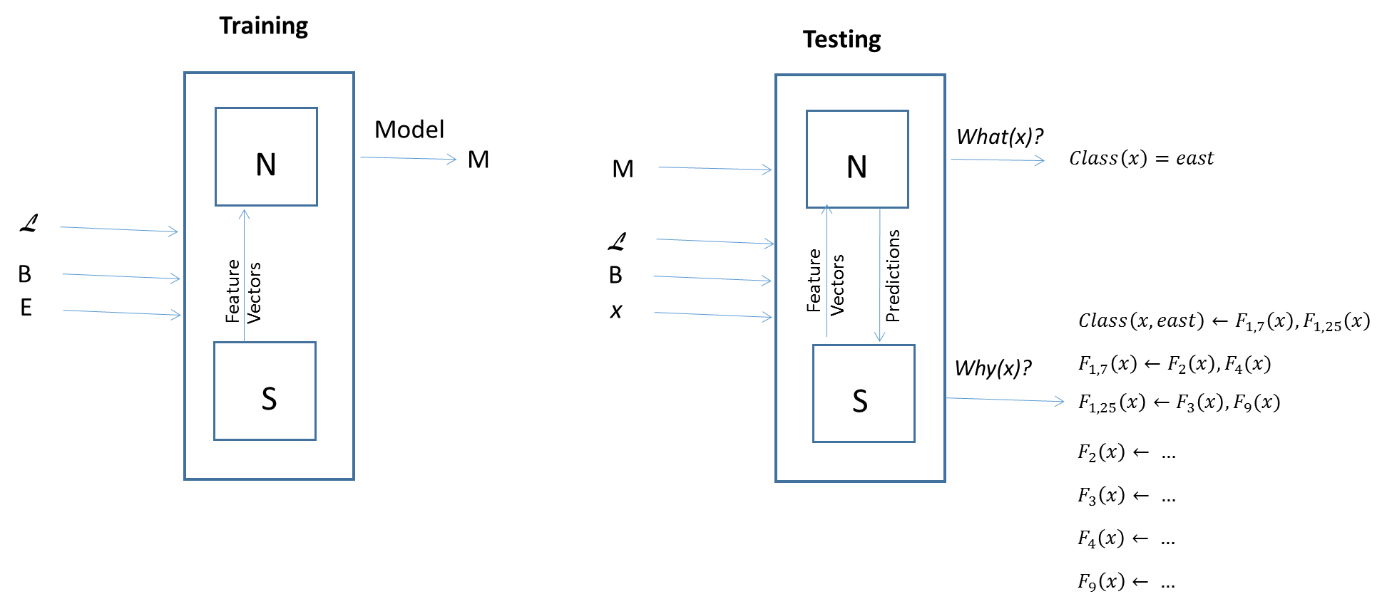
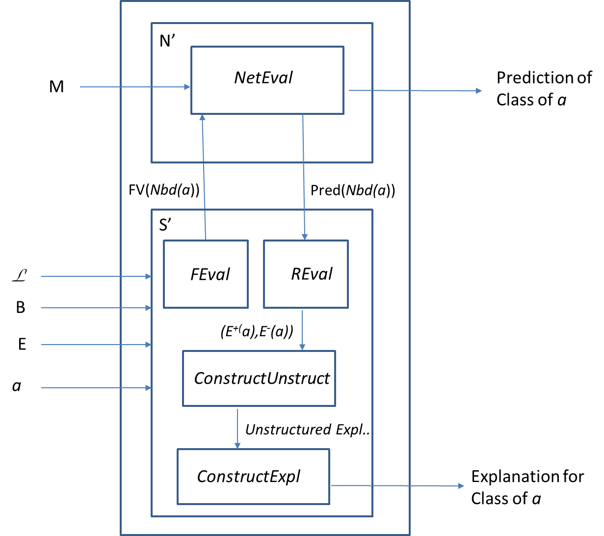
Our interest here therefore is in investigating the use of separate models for prediction and explanation. Specifically, we examine the use of a neural model for prediction, and a logical model for explanation. But in order to ensure that the models are about the same kinds of things, the models are not constructed independent of each other. The neural model is constructed in terms of features in (first-order) logic identified by a simple form of propositionalization methods developed in ILP. In turn, the predictions of the neural model are used to construct logical models in terms of the features. Figure 1 shows how the various pieces we have just described fit together.

Figure 1: What this paper is about. $N$ is a deep neural network, and $S$ is a symbolic learner. $B$ is domain-specific background knowledge; ${\cal L}$ language constraints; $E$ a set of training examples. $N$ is used to construct a predictive model $M$. Explanations of why $M$ predicts the class of a test instance $x$ are to be obtained as a logical model that uses features, that are pre-defined in $B$ or “invented”. Correctly, $B$ and ${\cal L}$ on the right are augmentations of those on the left; and the $S$’s on right and left are different instantiations of a first-order symbolic learner that is capable of producing definitions of features (left), or explanations (right).

Having two separate models would appear to be an extravagance that could be ill-afforded if the neural model wasn’t a very good predictor, or if the logical model wasn’t a very good explainer. In this paper, we present empirical evidence that neither of these appears to happen here. For ML practitioners, the principal points of interest in the paper are these:

1. We present a simple randomised method for obtaining first-order features that use domain-knowledge for use by a deep neural network. The resulting deep relational machine, or DRM, achieves high predictive performance, with small numbers of data instances. This extends existing work on DRMs, which have in the past required the use of a full-fledged ILP engine for feature-selection [21]; and

2. We present a method for extracting local symbolic explanations for predictions made by the DRM by employing a Bayes-like trade-off of likelihood and prior preference. The latter is obtained using domain-knowledge of relevance of predicates used in the explanations. This extends the techniques proposed in [33] in the direction of making explanations both more expressive (by using first-order logic) and meaningful (by using a Bayes-like method of incorporating domain-specific preferences into explanations).

The rest of the paper is organised as follows. In Section 2 we describe the DRMs we use for prediction. Section 3 describes the notion of explanations as used in this paper. Selection amongst several possible explanations is in Section 4, which introduces the use of a relevance-based prior in Section 4.1. Section 5 presents an empirical evaluation of the predictive and explanatory models, using some benchmark datasets. Appendix Logical Explanations for Deep Relational Machines Using Relevance Information contains details of the domain-specific relevance information used in the experiments.

2 A Deep Relational Machine for Prediction

One of the most remarkable recent advances in the area of Machine Learning is a resurgence of interest in neural networks, resulting from the automated construction of “deep networks” for prediction. Simplistically, Deep Learning is using neural networks with multiple hidden layers. Mathematically speaking, it is a composition of multiple simple non-linear functions trying to learn a hierarchy of intermediate features that most effectively aid the global learning task. Learning such intermediate features with neural networks has been made possible by three separate advances: (a) mathematical techniques that allow the training of neural networks with very large numbers of hidden layers; (b) the availability of very large amounts of data that allow the estimation of parameters (weights) in such complex networks; and (c) the advanced computational capabilities offered by modern day GPUs to train deep models. Despite successes across a wide set of problems, deep learning is unlikely to be sufficient for all kinds of data analysis problems. The principal difficulties appear to lie in the data and computational requirements to train such models. This is especially the case if many hidden layers are needed to encode complex concepts (features). For many industrial processes, acquiring data can incur significant costs, and simulators can be computationally very intensive.

Some of this difficulty may be alleviated if knowledge already available in the area of interest can be taken into account. Consider, for example, a problem in the area of drug-design. Much may be known already about the target of interest: small molecules that have proved to be effective, what can and cannot be synthesized cheaply, and so on. If these concepts are relevant to constructing a model for predicting good drugs, it seems both unnecessary and inefficient to require a deep network to re-discover them (the problem is actually worse — it may not even be possible to discover the concepts from first-principles using the data available). It is therefore of significant practical interest to explore ways in which prior domain-knowledge could be used in deep networks to reduce data and computational requirements.

Deep Relational Machines, or DRMs, proposed in [21], are deep neural networks with first-order Boolean functions at the input layer (“function $F_{1}$ is true if the instance $x$ is a molecule containing a 7-membered ring connected to a lactone ring” — definitions of relations like 7-membered and lactone rings are expected to be present in the background knowledge). In [21] the functions are learned by an ILP engine. This follows a long line of research, sometimes called propositionalization, in which features constructed by ILP have been used by other learning methods like regression, decision-trees, SVMs, topic-models, and multiplicative weight-update linear threshold models. In each of these, the final model is constructed in two steps: first, an ILP engine constructs a set of “good” features, and then, the final model is constructed using these features, possibly in conjunction with other features already available. Usually the models show significant improvements in predictive performance when an existing feature set is enriched in this manner. In [21], the deep network with ILP-features is shown to perform well, although the empirical evidence is limited. For the DRMs used in this paper we dispense with the requirement for an ILP-based selection of input features. Instead we use random selections of features generated from a space that has some constraints on logical relevance and redundancy. We will continue to refer to this kind of model as a DRM, since the features are still first-order Boolean functions defined in terms of relations provided as background knowledge.

2.1 First-Order Features as Inputs

In this paper, we do not want to pre-select input features using an ILP engine. Instead, we would (ideally) like the inputs to consist of all possible relational features, and let the network’s training process decide on the features that are actually useful (in the usual manner: a feature that has 0 weights for all out-going edges is not useful). The difficulty with this is that the number of such features in first-order logic can be very large, often impractical to enumerate completely. We clarify first what we mean by a relational feature.

Definition 1

Relational Examples for Classification. The set of examples provided can be defined as a binary relation $\mathit{Class}$ which is a subset of the Cartesian product ${\cal X}\times{\cal Y}$ where ${\cal X}$ denotes the set of relational instances (for simplicity, and without loss of generality, we will take each instance to be a ground first-order term) and ${\cal Y}$ denotes the finite set of class labels. Any single element of the set of relational examples will be denoted by $Class(a,c)$ where $a\in{\cal X}$ and $c\in{\cal Y}$.

Definition 2

Relational Features. A relational feature is a unary function $F_{i}:{\cal X}\mapsto\{\mathit{TRUE},\mathit{FALSE}\}$ defined in terms of a conjunction of predicates ${Cp}_{i}(x)$. Each predicate in ${Cp}_{i}(x)$ is defined as part of domain- or background-knowledge $B$. That is, $F_{i}(x)\mapsto\mathit{TRUE}$ iff ${Cp}_{i}(x)\mapsto\mathit{TRUE}$ and $\mathit{FALSE}$ otherwise. We will represent each relational feature as a single definite clause $\forall x\;(F_{i}(x)\leftarrow{Cp}_{i}(x))$ in a logic program, relying on the closed-world assumption for the complete definition of $F_{i}$. We will sometimes call the relational feature $F_{i}$ simply the feature $F_{i}$, and the definite-clause definition for $F_{i}$ the feature-definition for $F_{i}$. If the feature-definition of $F_{i}$ is in $B$, we will sometimes say “feature $F_{i}$ is in $B$.” We will usually denote the set of features in $B$ as ${\cal F}_{B}$ or simply ${\cal F}$.

Definition 3

Classification clause. A clause for classifying a relational example $Class(a,c)$ is a clause $\forall x(Class(x,c)\leftarrow{Cp}(x))$, where ${Cp}(x)$ is a conjunction of predicates. Each predicate in ${Cp}(x)$ is defined as part of domain- or background-knowledge $B$.

It is evident from the definitions that some or all of a classification clause can be converted into relational features.

Example 4

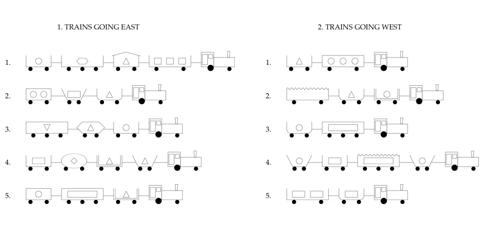
The trains problem. A well-known synthetic problem in the ILP literature (Michalski’s “Trains” problem, originally posed in [24] – see Fig. 2) can be used to illustrate this For this problem each relational example is a pair, consisting of a ground first-order term and a class label. The ground term represents the train (for example $Train(Car(Long,$ $Open,Rect,3),$ $Car(Short,Closed,Triangle,1),$ $\ldots)$) and the label denotes whether or not it is Eastbound.

We assume also that we have access to domain (or background) knowledge $B$ that allows us to access aspects of the relational instance such as $Has\_Car(Train(\ldots),$ $Car(\ldots))$, $Closed(Car(\ldots))$ and so on. Then a clause for classifying Eastbound trains is (we leave out the quantifiers for simplicity):

$$Class(x,East)\leftarrow Has\_Car(x,y),Short(y),Closed(y)$$

Here ${Cp}(x)$ = $Has\_Car(x,y)\wedge Short(y)\wedge Closed(y)$. The following relational features can be obtained from this classification clause:

$$F_{1}(x)\leftarrow Has\_Car(x,y),Short(y)$$

and:

$$F_{2}(x)\leftarrow Has\_Car(x,y),Closed(y)$$

The classification clause could now be written as:

$$Class(x,c)\leftarrow F_{1}(x),F_{2}(x)$$

Definition 5

Feature Vector of a Relational Instance. For a set of features ${\cal F}$ ordered in some canonical sequence $(F_{1},F_{2},\ldots,F_{d})$ we obtain a Boolean-vector representation $a^{\prime}\in\{0,1\}^{d}$ of a relational instance $a\in{\cal X}$ using the function $FV:{\cal X}\rightarrow\{0,1\}^{d}$, where the $i^{\mathrm{t}h}$ component ${FV}_{i}(x)$ = 1 if $F_{i}(x)\mapsto\mathit{TRUE}$, and 0 otherwise. We will sometimes say $a^{\prime}$ is the feature-space representation of $a$.

Figure 2: Michalski’s trains problem. There are two sets of trains: Eastbound and Westbound. Descriptors for the trains include: number, shape and lengths of the car, shape of load, and so on. The task is to determine classification rules to distinguish Eastbound trains from Westbound ones.

2.2 Logical Relevance and Redundancy of Features

So far, features have been defined purely syntactically. This is usually not sufficient to ensure that a feature in the class is relevant to the problem considered, or that it is redundant given another feature. For example, the feature $F_{1}$ defined by the clause $F_{1}(x)\leftarrow Has\_Car(x,y),Open(y),Closed(y))$ is clearly irrelevant in the trains problem, since no car can be both open and closed; and the feature $F_{3}$ defined by the clause $F_{3}(x)\leftarrow Has\_Car(x,y),$ $Short(y),Closed(y)$ is redundant given a feature-definition $F_{2}(x)\leftarrow~{}Has\_Car(x,y),$ $Closed(y),Short(y)$.

In their full scope, both irrelevance and redundancy of features are semantic notions dependent on domain knowledge. Since features are defined by clauses, in this paper we will use approximations based on the well-understood concept of clause subsumption from the ILP literature, the main definitions of which we reproduce here for completeness:

Definition 6

Clause subsumption. We use Plotkin’s partial ordering on the set of clauses [32]. A clause $C$ subsumes a clause $D$ or $C\preceq_{\theta}D$, iff there exists a substitution $\theta$ s.t. $C\theta\subseteq D$. It is known that if $C\preceq_{\theta}D$ then $C\models D$. Further if $C\preceq_{\theta}D$ and $D\preceq_{\theta}C$ we will say $C\equiv_{\theta}D$.

Remark 7

Most specific clause in a depth-bounded mode language. This notion is due to Muggleton [28]. Given a set of modes $M$, let ${\cal L}_{d}(M)$ be the $d$-depth mode language. Given background knowledge $B$ and an instance $e$, let the most specific clause that logically entails $e$ in the sense described in [28] be $\bot(B,e)$. For every $\bot(B,e)$ it is shown in [28] that: (a) there is a $\bot_{d}(B,e)$ in ${\cal L}_{d}(M)$ s.t. $\bot_{d}(B,e)\preceq\bot(B,e)$; and (b) $\bot_{d}(B,e)$ is finite.

Using these notions, we adopt the following definitions:

Definition 8

Logical relevance. Given a set of examples $E$, and background knowledge $B$, an independent clause $C$ is relevant if $C\preceq\bot_{d}(B,e)$ for at least one $e\in E$. We will further restrict this to $C\subseteq\bot_{d}(B,e)$.

Definition 9

Logical redundancy. For a pair of independent clauses $C$ and $D$, we will say $D$ is redundant given $C$ (and vice-versa), if $|C|=|D|$ and $C\equiv_{\theta}D$.

These definitions based on subsumption are an approximation to the true logical definitions of relevance and redundancy, and can result in some errors (assuming relevance when it does not exist, and missing redundancy when it does exist). Nevertheless, they can be computed reasonably efficiently. They form the basis of a method of randomised construction of inputs for the deep network.

2.3 Randomised Feature Selection

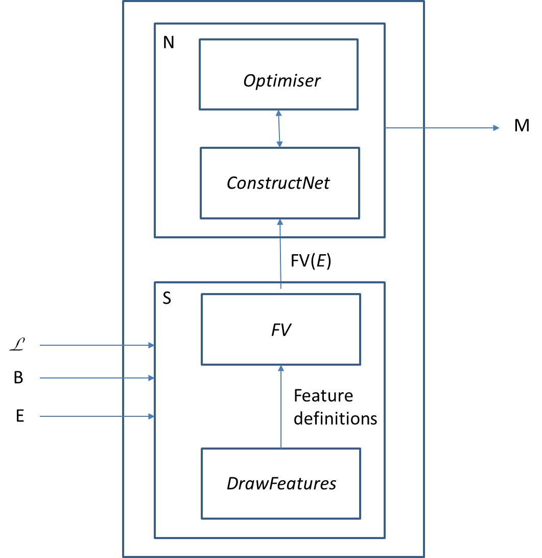
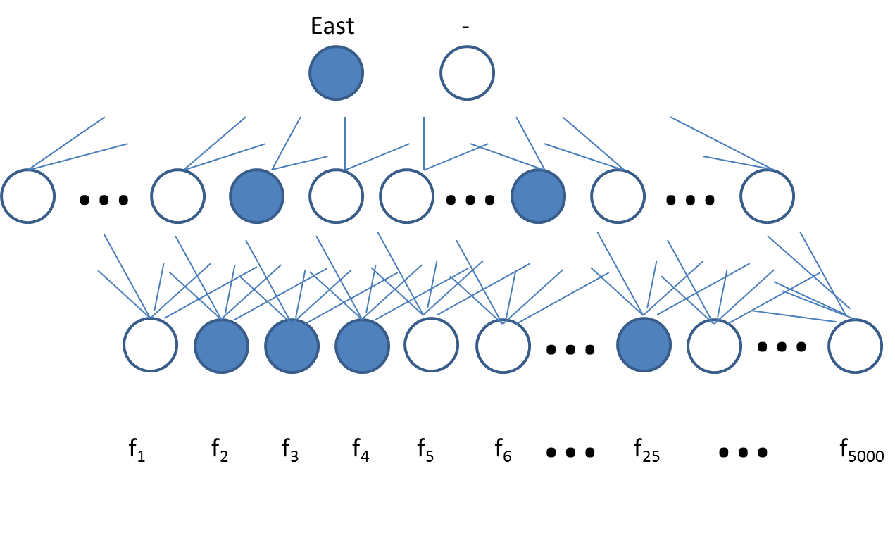
The mechanisms for detecting logical relevance and redundancy help to reduce the number of possible features within a mode language. But they still do not guarantee that the numbers will be manageable. We therefore resort to a rejection-based sampling strategy for selecting inputs (Fig. 3). Of course, inputs to the DRM are not the features themselves but the feature-space representations for the relational instances in $E$ (Fig. 4).

$DrawFeatures(B,E,{\cal M},{\cal L},d,MaxDraws):$

Given:

Background knowledge $B$; examples $E$; a set of modes ${\cal M}$; language constraints ${\cal L}$; a depth-bound $d$; and an upper-bound on the number of samples $MaxDraws$.

Find:

A set of features ${\cal F}$ s.t. $|{\cal F}|\leq MaxDraws$

1. Let $F=\emptyset$

2. Let $draws=0$

3. Let $i=1$

4. Let $Drawn$ be $\emptyset$

5. while $draws\leq MaxDraws$ do

   1. Randomly draw with replacement an example $e_{i}\in E$. Let $e_{i}=Class(a,c)$, where $a$ is a relational instance and $c$ is a class label.

   2. Let $\bot_{d}(B,e_{i})$ be the most specific clause in the depth-limited mode language ${\cal L}_{d}({\cal M})$ that subsumes $\bot(B,e_{i})$ (i.e., the most-specific clause that entails $e_{i}$, given $B$).

   3. Randomly draw a clause $C_{i}$ s.t. $C_{i}\subseteq\bot_{d}(B,e_{i})$

   4. if ($C_{i}$ is not redundant given $Drawn$) then

      1. Let $C_{i}=(Class(x,c)\leftarrow{Cp}_{i}(x))$

      2. Let $F_{i}=(F_{i}(x)\leftarrow{Cp}_{i}(x))$

      3. $F~{}:=~{}F\cup\{F_{i}\}$

      4. $Drawn~{}:=~{}Drawn\cup\{C_{i}\}$

      5. increment $i$

   5. increment $draws$

6. done

7. return $F$

Figure 3: A randomised procedure for drawing features from a depth-limited mode language. A procedure for randomly drawing clauses subsuming a most-specific clause required in Step 5c is described in [43].

Figure 4: More details on the training component in Fig. 1. For simplicity, we are taking the modes ${\cal M}$ to be part of the language specification ${\cal L}$, and do not show some parameters. The optimiser finds the best network structure and parameters using the feature-vectors provided for training. FV($E$) denotes the feature-vectors of the relational instances $E$. The model $M$ is a DRM.

3 Logical Explanations for Predictions by a DRM

Predicting the class-label of a relational instance $a$ using the model $M$ in Fig. 4 is a 2-step process: (1) The feature-vector representation $a^{\prime}$ of $a$ is obtained using the feature-definitions found during the training stage; and (2) $a^{\prime}$ is provided as input to the model $M$ found during training, which then computes the class-label (Fig. 5).

Figure 5: Prediction of the class of a relational instance $a$ by a DRM. The inputs $f_{i}$ are the component values of the feature-vector ${FV}_{i}(a)$. The shaded inputs denote a feature-value of 1. With a DRM, there is more to $f_{i}=1$ than just an assignment of $1$ to feature: it also means that some conjunction of background predicates ${Cp}_{i}(a)$ is TRUE for the relational instance $a$. The shaded circles in hidden layers denote activated nodes. The shaded output node denotes the prediction of the relational instance is $East$.

It has long been understood that neural models can compute accurate answers for questions like “What is the prediction for x?”. But what can be said about why the answer is what it is? Unsurprisingly, there has been a lot of research effort invested into extracting explanations for the predictions made by a neural network (see [8], Chapter 3 for a full description of this line of research). Most of this effort has been in the direction of translating the network into a single symbolic model that guarantees correspondence to the neural model (for example, [42]). Alternatively, a single symbolic model can be learned that approximates the behaviour of the neural model over all inputs (for example, [5]). Although distinct in their aims, both approaches still result in two separate models, one neural and the other symbolic. In both cases the symbolic model is intended to be a readable proxy for the neural model, which can then form a basis for an explanation of “why” questions. But there are some inherent trade-offs:

• If we try to replicate exactly the behaviour of the neural network with a symbolic model (as is done, say, in [42]), then the resulting model may not be any more comprehensible than the neural network; and

• If we try only to approximate the behaviour of the network using logical predicates (as is done, say, in [5]), then we run the risk of not being able to replicate the network’s behaviour sufficiently accurately over all instances, because of inadequacies of the logical predicates available.

Both these issues are exacerbated for modern-day deep networks, with many hidden layers and large numbers of inputs. One way to side-step these difficulties is simply to drop the requirement of translating the entire network model into a single symbolic model. Recent research called LIME (“Local Interpretable Model-agnostic Explanations”: [33]) proposes producing readable proxies “on-demand”, for any kind of black-box predictor. The key feature is that a LIME-style explanatory model is constructed only when a prediction for an instance is sought, and the explanation is required to be faithful to the black-box’s (in our case, a neural network) predictions for the instance and its near-neighbours. The intuition is that while comprehensible models may not be possible for the entire black-box model, they may be possible when restricted to local predictions.

The requirement of having to be consistent with only local instances results in a different kind of problem. Since the near-neighbours of an instance may be quite small, there may be insufficient constraints, in data-theoretic terms, to narrow down on a unique (or even a small number of) explanations. So, how then is an explanation to be selected? In LIME, this is left to the loss-function. In Bayesian terms, this means defining an appropriate prior to guide selection when the data are insufficient.

3.1 Local Explanations

We now consider a logical formulation of the setting introduced in the LIME paper that is well-suited to explaining DRM models. We draw on specific situations described in [27], namely to clarify what is meant by a local explanation, and its data-theoretic evaluation. Later we will introduce a domain-dependent prior to develop a Bayes-like selection of interpretable explanations.

Definition 10

Explanations. In this paper, we will only be concerned with explanations for the classification of an instance. As before, we assume a set of relational instances ${\cal X}$, and a finite set of classes ${\cal Y}$. Given a relational instance $a\in{\cal X}$ and a label $c\in{\cal Y}$, the statement $Class(a,c)$ will denote that the class of $a$ is $c$. Let $e=Class(a,c)$. Then given background knowledge $B$, an explanation for $e$ is a set of clauses $H$ s.t. $B\cup H\models e$.

At this point, we differ from Good [11], for whom it is neither necessary nor sufficient for good explanations to logically imply $e$, given $B$. As we present it here, logical implication is necessary, but as will be seen below, not sufficient for a good explanation. We will seek explanations of a restricted kind, namely those defined in terms of features.

Definition 11

Feature-clauses. Let ${\cal F}$ be a set of features. A definite clause is said to be a feature-clause if all negative literals are of the form $F_{i}(x)$, where the $F_{i}$ are in ${\cal F}$ and the $x$ is universally quantified.

3.1.1 Single-Clause Explanations

Assume we have a set of $d$ features ${\cal F}$ with corresponding feature-definitions in the background knowledge $B$. We will first consider the case where explanation $H$ consists of a single feature-clause. That is, $H=\{C\}$, where $C$ is a definite clause $\forall x\;(Class(x,c)\leftarrow Body)$. Here $Body$ is a conjunction of ${F}_{i}/1$ literals, each of which is defined in $B$. The ILP practitioner will recognise that finding a single feature-clause explanation for $Class(a,c)$ is an instance of the “Single example clause, single hypothesis clause” situation identified in [27], which forms the basis of explanation-based learning (EBL) [26].

Example 12

An explanation in the trains problem. An explanation $H=\{C\}$ for the first train in the left column of Fig. 2 is the feature-clause:

$$C:Class(t1,East)\leftarrow{F}_{1}(t1),{F}_{2}(t1),{F}_{3}(t1)$$

where $B$ contains:

$$\forall x({F}_{1}(x)\leftarrow\exists y(Has\_Car(x,y),Short(y)))$$

$$\forall x({F}_{2}(x)\leftarrow\exists y(Has\_Car(x,y),Closed(y)))$$

$$\forall x({F}_{3}(x)\leftarrow\exists y(Has\_Car(x,y),Long(y)))$$

Here $t1$ is used as short-form for a structured term, describing the train, and, as before, let us assume that appropriate definitions exist in $B$ for predicates like $Has\_Car$, $Long$, $Short$, and $Closed$ to succeed (or fail) on terms like $t1$.

One explanation for $e=Class(a,c)$ can be obtained immediately as follows. Consider the set $F_{a}=\{F_{i}:F_{i}\in{\cal F}~{}\mathrm{s.t.}~{}{FV}_{i}(a)=1\}$ (let us call these the set of active features for $a$). By definition, if ${FV}_{i}(a)=1$ then $F_{i}(a)\mapsto\mathit{TRUE}$. For simplicity, let us suppose that $F_{a}$ = $\{F_{1},\ldots F_{k}\}$ is the set of active features for $a$, and let $C:~{}Class(a,c)\leftarrow{F}_{1}(a),{F}_{2}(a),\ldots,{F}_{k}(a)$. Assuming the $F_{i}$ are defined in $B$, $H~{}=~{}\{C\}$ is an explanation for $e$. Fig. 6 is a simple procedure to construct a single-clause explanation $C^{\prime}$ that relies on the result that if $C^{\prime}\preceq_{\theta}C$, then $C^{\prime}\models C$. Therefore, if $B\cup\{C\}\models e$, then evidently $B\cup\{C^{\prime}\}\models e$. That is, $\{C^{\prime}\}$ will also be an explanation for $e$. For reasons that will be apparent, we will call $\{C^{\prime}\}$ an “unstructured” explanation.

$ConstructUnstruct(e,B,{\cal F}):$

Given:

A relational instance $e$; background knowledge $B$; a set of features ${\cal F}$ with definitions in $B$.

Find:

A single feature-clause explanation $H$ s.t. $B\cup H\models e$.

1. Let $e=Class(a,c)$

2. Let $a^{\prime}=FV(a)$

3. Let ${\cal F}^{\prime}$ be the set of features that map to $TRUE$ in $a^{\prime}$

4. Let ${\cal H}$ be the subset-lattice of ${\cal F}^{\prime}$

5. Let $F^{\prime}$ be any element in ${\cal H}$ s.t.

   • $Body$ is the conjunction of features in $F^{\prime}$;

   • $C^{\prime}=\forall x(Class(x,c)\leftarrow Body)$

6. return $\{C\}$

Figure 6: A procedure for identifying a single-clause unstructured explanation.

3.1.2 Multi-Clause Explanations

We now extend explanations to a restricted form of multi-clause explanations, which use features that are not all defined in the background knowledge $B$. We will require these “invented” features to be (re-)expressible in terms of features already defined in $B$. In this paper we will require structured and unstructured explanations to be related by the logic-program transformation operations of folding and unfolding. That is, given an unstructured explanation $H$ and a structured explanation $H_{1}$, $H$ can be derived from $H_{1}$ using one or more unfolding transformations; and $H_{1}$ can be derived from $H$ using one or more folding transformations. We describe the transformations, along with the conditions that ensure that the computable answers do not change when the transformation is applied.

Definition 13

(One-Step) Unfolding of a clause [13]. Given a set of definite clauses $P$, W.l.o.g. let $C\in P$ s.t. $C$ = $Head\leftarrow L_{1},\ldots,L_{i},\ldots,L_{k}$ ($k\geq 1$). Let $C^{\prime}$ be a clause ${L^{\prime}}_{i}\leftarrow{Body}^{\prime}$ s.t. $L_{i}$ and ${L^{\prime}}_{i}$ unify with m.g.u $\theta$. Then the (one-step) unfolding of $C$ w.r.t $L$ using $P$ is the clause $Unfold(C):(Head\leftarrow L_{1},\ldots,L_{i-1},{Body}^{\prime},L_{i+1},\ldots,L_{k})\theta$

Definition 14

(One-Step) folding of a clause [13]. Given a set of definite clauses $P$, W.l.o.g. let $C\in P$ s.t. $C$ = $Head\leftarrow L_{1},\ldots,{L_{i-1},Body}_{i},L_{i+1},\ldots,L_{k}$, where ${Body}_{i}$ is some literals $B_{1},B_{2},\ldots,B_{j}$ ($j,k\geq 1$). Let $C^{\prime}$ be a clause ${L^{\prime}}_{i}\leftarrow{Body}^{\prime}$ s.t. there is a substitution $\theta$ that satisfies: (a) ${Body}_{i}={Body}^{\prime}_{i}\theta$; (b) Every existentially quantified variable $y$ in $C$, $y\theta$ is a variable that occurs only in ${Body}_{i}$ and nowhere else; (c) For any pair of distinct existential variables $y,z$ in $C$ $y\theta\neq z\theta$; and (d) $C^{\prime}$ is the only clause in $P$ whose positive literal unifies with ${L^{\prime}}_{i}\theta$. Then the (one-step) unfolding of $C$ w.r.t. ${Body}_{i}$ using $P$ is the clause $Fold(C):(Head\leftarrow L_{1},\ldots,L_{i-1},{L^{\prime}}_{i}\theta,L_{i+1},\ldots,L_{k})$.

Remark 15

Correctness of Transformations. In [10] the unfold and fold transformations are defined above are shown to be correct as replacement rules w.r.t. the minimal-model (MM) semantics. That is, if $P$ is a definite-clause program and $C\in P$, then $MM(P)$ = $MM((P-\{C\})\cup Trans(C))$, where $Trans(C)$ is $Fold(C)$ or $Unfold(C)$.

We use this to construct structured explanations that are correct, in the computational sense just identified. That is, a structured explanation can replace an unstructured explanation without altering the minimal model of the (program containing) the unstructured explanation. It is convenient for us to introduce the notion of an “invented” feature.

Definition 16

Invented Feature. Given background knowledge $B$, a feature $F$ is said to be an invented feature if: (1) $F$ is not defined in $B$; and (2) The definition of $F$ is a feature-clause $C$ whose body contains features in $B$ only; or is a clause that unfolds to a feature-clause $C$ containing features only in $B$. We will sometimes denote $C$ as $UFC(F)$ (short for “unfolded feature-clause for F”).

Example 17

Invented features in the trains problem. The features $F_{1,1}$ and $F_{1,2}$ are invented features:

${F}_{1,1}(x)\leftarrow{F}_{2}(x),{F}_{1,2}(x)$

${F}_{1,2}(x)\leftarrow{F}_{4}(x),{F}_{9}(x)$

where the $F_{i}$ are features defined in background knowledge:

${F}_{2}(x)\leftarrow Has\_Car(x,y),Short(y)$

${F}_{4}(x)\leftarrow Has\_Car(x,y),Wheels(y,3)$

${F}_{9}(x)\leftarrow Has\_Car(x,y),Load(y,triangle)$

Then $UFC(F_{1,1})$ is:

$$F_{1,1,}(x)\leftarrow F_{2}(x),F_{4}(x),F_{9}(x)$$

and $UFC(F_{1,2})$ is identical to the definition of $F_{1,2}$.

We distinguish between unstructured and structured definitions based on the presence or absence of invented features.

Definition 18

Unstructured and structured explanations. Let $a\in{\cal X}$ and ${\cal Y}$ be a set of class labels, with $c\in{\cal Y}$. Let $N:\Re^{d}\rightarrow{\cal Y}$ be a predictive model such that $N(FV(a))=c$. Given background knowledge $B$, let $H$ be an explanation for $Class(a,c)$ containing the feature-clause $C:\forall x(Class(x,c)\leftarrow Body)$. Let $Body$ consist of features ${\cal F}_{C}$. Let ${\cal F}_{C}$ be partitioned into: (a) ${\cal F}_{C,old}$, consisting of features defined in $B$; and (b) ${\cal F}_{C,new}$, consisting of features defined in $H-B$.

We will call $H$ an unstructured explanation iff: (1) ${\cal F}_{C}$ contains only old features (that is, ${\cal F}_{C,new}=\emptyset$); and (2) $H$ = {C}.

We will call $H$ a structured explanation iff: (1) ${\cal F}_{C}$ contains only invented features (that is, ${\cal F}_{C,old}=\emptyset$); and (2) $H=\{C\}\cup InvF$, where $InvF$ pnly contains clauses defining invented features in ${\cal F}_{C,new}$; (3) Each feature $F$ in ${\cal F}_{C,new}$ there is a single clause definition in $InvF$, s.t. $F$ unfolds to a unique feature-clause defined using features in $B$ only; and (4) At least one $F\in{\cal F}_{C,new}$ unfolds to a feature-clause that contains at least 2 features from $B$ (that is, there is at least one invented feature that is not a trivial rewrite of features in $B$).

That is, a structured explanation is a set of clauses containing a classification clause $C$ along with definitions of invented features (and thus is a case of the “single example clause, multiple hypothesis clauses” situation in [27]).

Example 19

Unstructured and structured explanations for the trains problem. Suppose we are given an instance $a\in{\cal X}$, and a set of features ${\cal F}$, each defined by feature-definitions in background $B$. Then we will call the following an unstructured explanation ($x$ is universally quantified):

$$C:Class(x,East)\leftarrow{F}_{2}(x),{F}_{3}(x),{F}_{4}(x),{F}_{9}(x)$$

The following is a structured explanation $H_{1}$:

$Class(x,East)\leftarrow{F}_{1,1}(x),{F}_{1,2}(x)$

${F}_{1,1}(x)\leftarrow{F}_{2}(x),{F}_{3}(x)$

${F}_{1,2}(x)\leftarrow{F}_{4}(x),{F}_{9}(x)$

Note that $H_{1}$ unfolds to $H$. Another structured explanation that also unfolds to $H$ is $H_{2}$ below:

$Class(x,East)\leftarrow{F}_{1,1}(x),{F}_{1,2}(x)$

${F}_{1,1}(x)\leftarrow{F}_{1}(x),{F}_{4}(x)$

${F}_{1,2}(x)\leftarrow{F}_{3}(x),{F}_{9}(x)$

We will assume that explanations of the form $Class(x,East)\leftarrow{F}_{1,1}(x),{F}_{3}(x),{F}_{9}(x)$ will be represented as $H_{2}$. Also, by definition, the following is not a structured explanation, since all new features are trivial rewrites of existing ones:

$Class(x,East)\leftarrow{F}_{1,1}(x),{F}_{1,2}(x)$

${F}_{1,1}(x)\leftarrow{F}_{1}(x)$

${F}_{1,2}(x)\leftarrow{F}_{3}(x)$

But this is a structured explanation:

$Class(x,East)\leftarrow{F}_{1,1}(x),{F}_{1,2}(x)$

${F}_{1,1}(x)\leftarrow{F}_{1}(x)$

${F}_{1,2}(x)\leftarrow{F}_{3}(x),{F}_{9}(x)$

It is obvious enough that the unfolding step that every structured explanation allows the derivation of a correct unstructured explanation.

Remark 20

Deriving an Unstructured Explanation from a Structured Explanation. Let $H=\{C^{\prime}\}\cup InvF$ be a structured explanation for a relational example $Class(a,c)$ given background knowledge $B$. W.l.o.g. from Defn. 18, $C^{\prime}$ is a clause $Class(x,c)\leftarrow\{{F^{\prime}}_{1}(x),{F^{\prime}}_{2}(x),\ldots,{F^{\prime}}_{k}(x)$ s.t. each ${F^{\prime}}_{i}$ unfolds using $InvF$ to a unique feature-clause ${F^{\prime}}_{i}(x)\leftarrow F_{i,1}(x),\ldots,F_{i,n_{i}}(x)$, where the $F_{i,\cdot}$ are defined in $B$. From Defn.13, unfolding $C^{\prime}$ w.r.t. the ${F^{\prime}}_{i}$ using $InvF$ results in the clause $C:~{}Class(x,c)\leftarrow F_{1,1},\ldots,F_{k,n_{k}}$. From Remark 15, the minimal model of $B\cup H$ will be unchanged by replacing $C^{\prime}$ with $C$. It follows that $H$ = $\{C\}$ is an unstructured explanation for $Class(a,c)$ that is computationally equivalent to $H^{\prime}$.

One or more correct structured explanations follow from an unstructured if the conditions in Defn.14 hold. Constraints on the invented features can ensure this.

Remark 21

Deriving Structured Explanations from an Unstructured Explanation. Let $H=\{C\}$ be an unstructured explanation for a relational example $Class(a,c)$ given background knowledge $B$. W.l.o.g. from Defn. 18, $C$ is a clause $Class(x,c)\leftarrow\{{F}_{1}(x),{F}_{2}(x),\ldots,{F}_{n}(x)$ s.t. each ${F}_{i}$ is defined in $B$. Let $InvF$ consist of $k$ features ${F^{\prime}}_{1},\ldots,{F^{\prime}}_{k}$ s.t. each ${F^{\prime}}_{i}$ is uniquely defined by features in a block of a $k$-partition of $F_{1},\ldots,F_{n}$. Let $C^{\prime}$ be the clause $Class(x,c)\leftarrow{F^{\prime}}_{1}(x),{F^{\prime}}_{2}(x),\ldots,{F^{\prime}}_{k}(x)$. Then $H^{\prime}=\{C^{\prime}\}\cup InvF$ is a structured explanation for $Class(a,c)$ that is computationally equivalent to $B\cup\{C\}\cup InvF$. This follows since the conditions (a)–(d) in Defn. 14 are trivially satisfied (condition (a) follows with $\theta$ being a simple renaming substitution; (b)–(c) follow since there are no existential variables in the definitions of the ${F^{\prime}}_{i}$; and (d) since there is a single clause definition for each feature in $InvF$).

Remark 21 suggests a straightforward non-deterministic procedure to construct a correct structured explanation (Fig. 7).

$ConstructStruct(H,B,k):$

Given:

An unstructured explanation $H$; background knowledge $B$; and a number $k$ ($\geq 2$)

Find:

A structured explanation $H^{\prime}$ that is computationally equivalent to $H$

1. Let $H$ = $\forall x(Class(x,c)\leftarrow Body)$

2. Let $F$ be the set of features in $Body$

3. Let $P_{k}$ be a set s.t:

   1. Either $P_{k}$ is a $k$-partition of $F$ s.t. at least one block in $P_{k}$ contains $2$ or more elements; or

   2. Or, $P_{k}=\emptyset$ (if no such $k$-partition exists)

4. If $P_{k}=\emptyset$ return $\emptyset$.

5. Otherwise:

   1. Let $P_{k}$ consist of blocks $b_{1},b_{2},\ldots,b_{k}$

   2. For each block $b_{i}\in P_{k}$:

      1. Construct a new feature ${F^{\prime}}_{i}$ with definition $C_{i}$ = $\forall x({F^{\prime}}_{i}(x)\leftarrow{Body}_{i})$, where ${Body}_{i}$ is the conjunction of the features in $b_{i}$

   3. Let $C_{0}$ = $\forall x(Class(x,c)\leftarrow{Body}_{0})$ where ${Body}_{0}$ is the conjunction of the ${F^{\prime}}_{1},{F^{\prime}}_{2},\ldots,{F^{\prime}}_{k}$

   4. Let $H^{\prime}$ = $\bigcup_{i=0}^{k}C_{k}$

6. Return $H^{\prime}$.

Figure 7: A procedure for obtaining a structured explanation from an unstructured explanation, by inventing $k$ features. The condition in Step 3 is not required by Remark 21, but prevents inventing features that are trivial rewrites of existing features (see Defn. 18).

All explanations so far have only been required to explain a single relational instance. We extend this to explain the prediction by a black-box classifier of relational instances that are “close” to each other. This is the requirement identified in LIME [33]. Readers familiar with the ILP literature will recognise the task of finding such local explanation as as corresponding to either “Multiple examples, single hypothesis clause” or “Multiple examples, multiple hypothesis clauses” situations identified in [27] (depending on whether unstructured or structured explanations are constructed).

3.2 Local Explanations for a Black-Box Predictor

We are specifically interested in constructing explanations for the classification of an instances resulting from some (opaque) predictive model.

Definition 22

Explanation for a prediction by a model. Given a relational instance $a\in{\cal X}$ and a label $c\in{\cal Y}$. Assume we have a set of $d$ features ${\cal F}$. Given a predictive model $N:\Re^{d}\rightarrow{\cal Y}$, we will say $H$ is an explanation for $N(FV(a))=c$ if $H$ is an explanation for $e=Class(a,c)$.

We have just seen how to construct the most-specific feature-clause for $e=Class(a,c)$ from the set of active features for $a$. In fact, we will now want a little bit more from an explanation. Following [33], we will seek explanations that are not only consistent with a predictive model on an instance $x$, but be consistent with predictions made by the predictive model in a local neighbourhood of $x$.

Definition 23

Neighbourhood. Given relational instance $a\in{\cal X}$, and a set of $d$ features ${\cal F}$, and given some $\epsilon\in\Re$, we denote the neighbourhood of $a$ as $Nbd(a)~{}=~{}\{x:x\in{\cal X}~{}{\mathrm{a}nd}~{}{Dis}(FV(a),FV(x))\leq\epsilon\}$. Here $Dis$ is some appropriate distance measure defined over $d$-dimensional vectors.

In practice the dimensionality $d$ can be quite large, and since the standard Euclidean distance is known to be problematic in high-dimensional spaces [1] we will use an alternative measure.

Definition 24

Locally Consistent Explanations. Given relational instance $a\in{\cal X}$, and a predictive model $N$, let $N(FV(a))=c$. We define the following subsets of $Nbd(a)$: $E^{+}(a)=\{b:b\in Nbd(a)~{}{\mathrm{and}}~{}N(FV(b))=c)\}$ and $E^{-}(a)=\{b:b\in Nbd(a)~{}{\mathrm{and}}~{}N(FV(b))\neq c\}$. Then an explanation $H$ for $Class(a,c)$ given $B$ is a locally consistent explanation if: (1) for each $a^{\prime}\in E^{+}(a)$ $H$ is an explanation for $Class(a^{\prime},c)$ (that is, $B\cup H\models Class(a^{\prime},c)$); and (2) for each $a^{\prime}\in E^{-}(a)$ $B\wedge H\wedge\neg Class(a^{\prime},c)\not\models\Box$.

Example 25

Locally consistent explanation for the trains problem. For simplicity, we consider the situation where $E^{-}=\emptyset$. Suppose we now know that the local neighbourhood of the first train ($t1$) in the left column of Fig. 2 only contains the second train ($t2$) in that column. Let us assume that ${\cal F}$ consists just of the functions defined in Example 12. With those definitions, and a predictive model $N$, let $N(FV(t1))=N(FV(t2))$ ($=East$, say). Then $E^{+}(t1)=\{t1,t2\}$.

The most-specific feature-clause for $Class(t1,East)$ given ${\cal F}$ and $B$ is:

$$C1:Class(t1,East)\leftarrow{F}_{1}(t1),{F}_{2}(t1),{F}_{3}(t1)$$

and for $Class(t2,East)$ is:

$$C2:Class(t2,East)\leftarrow{F}_{1}(t2),{F}_{2}(t2)$$

where the function definitions are as before. Then a locally consistent explanation for $Class(t1,East)$ is the least-general-generalisation (or Lgg) of $C1$ and $C2$:

$$Lgg(C1,C2):\forall x(Class(x,East)\leftarrow{F}_{1}(x),{F}_{2}(x))$$

In general, $E^{-}\neq\emptyset$, and results from ILP tell us that it may not be possible to find a single clause that is locally consistent. We next describe a simple, qualitative form of Bayes Rule that combines likelihood of the data, with a relevance-based prior preference over explanations.

it is useful before we proceed further to have a numerical measure of the extent to which an explanation is locally consistent.

Definition 26

Fidelity. Let $a\in{\cal X}$. Given a predictive model $N$, let $N(FV(a))=c$ and $E^{+}(a)$, $E^{-}(a)$ as before. Let $D=(E^{+},E^{-})$ and $H$ be an explanation for $Class(a,c)$ given background knowledge $B$. Let: (1) $AgreePos(H)$ = $\{b:b\in E^{+}(a)$ and $B\wedge H\models Class(b,c)\}$; and (2) $AgreeNeg(H)$ = $\{b:b\in E^{-}(a)$ and $B\cup H\wedge\neg Class(b,c)\not\models\Box\}$. Then $\mathit{Fidelity}(H|D,B)=F_{H,a}=\frac{|AgreePos(H)|+|AgreeNeg(H)|}{|E^{+}(a)|+|E^{-}(a)|}$.

We note that $AgreePos(H)$ and $AgreeNeg(H)$ are the same as true positives and true negatives in the classification literature, and so fidelity is a localized form of accuracy (in [33] the term “local fidelity” is used for a localized form of error). We note also that if a structured explanation is derived from an unstructured one, then fidelity will not change.

Remark 27

Structuring preserves fidelity. Let $H^{\prime}=\{C^{\prime}\}\cup InvF$ be a structured explanation derived as in Remark 21 from an unstructured explanation $H=\{C\}$ for a relational example $Class(a,c)$, given definite-clauses $B$ and a predictor $N$ s.t. $N(FV(a))=c$. Let $E^{+}(a)$ and $E^{-}(a)$ denote relational examples obtained from the neighbourhood of $a$ as before, and $D=(E^{+}(a),E^{-}(a))$. Then, $Fidelity(H^{\prime}|D,B)=Fidelity(H|D,B)$.

Let $S$ be any finite set of ground $Class/2$ facts and $MM(P)$ be the minimal model of a definite-clause program $P$. Since $InvF$ is a definite-clause containing definitions of invented features, $S\cap MM(B\cup\{C\})=S\cap MM(B\cup\{C\}\cup InvF)$. Now, $AgreePos(H)$ = $\{Class(a^{\prime},c):Class(a^{\prime},c)\in(E^{+}(a)\cap MM(B\cup H)$ and $AgreeNeg(H)$ = $\{Class(a^{\prime},c):Class(a^{\prime},c)\in(E^{-}(a)-(E^{-}(a)\cap MM(B\cup H)$. Since $E^{+}(a)$ and $E^{-}(a)$ are finite set of ground $Class/2$ facts, and $H=\{C\}$, $AgreePos(H)$ = $\{Class(a^{\prime},c):Class(a^{\prime},c)\in(E^{+}(a)\cap MM(B\cup\{C\}\cup InvF)$ and $AgreeNeg(H)$ = $\{Class(a^{\prime},c):Class(a^{\prime},c)\in(E^{-}(a)-(E^{-}(a)\cap MM(B\cup\{C\}\cup InvF)$. From Remark 21, $MM(B\cup\{C\}\cup InvF)=MM(B\cup\{C^{\prime}\}\cup InvF)$. Since $H^{\prime}=\{C\}\cup InvF$, it follows immediately that $AgreePos(H)=AgreePos(H^{\prime})$ and $AgreeNeg(H)=AgreeNeg(H^{\prime})$ and therefore $Fidelity(H|D,B)=Fidelity(H^{\prime}|D,B)$. $\Box$

4 Selecting a Local Explanation

Given a relational instance $a\in{\cal X}$, let the prediction of $a$ by a DRM $N$ be $c$. But, for a definition of a neighbourhood, there may be several explanations for $Class(a,c)$ with the same maximal fidelity. How then should we select a single explanation? Provided we have some reasonable way of specifying prior-preferences, Bayes rule trades-off the fit to the data (likelihood) against prior preference (LIME’s minimisation of the sum of a loss and a regularisation term can be seen as implementing a form of Bayesian selection [33]).

A general setting for selecting amongst logical formulae is provided by labelled deductive systems (LDS: see [9]), in which logical formulae are extended with labels, with an associated algebra. For our purpose, it is sufficient simply to consider the comparison of labelled explanations.

Definition 28

Labelled Explanation. Given a relational example $e=Class(a,c)$, and background knowledge $B$, $\alpha:H$ is a labelled explanation for $e$ given $B$ if: (a) $H$ is an explanation for $e$ given $B$; and (b) $\alpha$ is a element of a partially-ordered set of ground first-order terms $\Delta$. $\Delta$ consists of annotations of all explanations for $e$ given $B$.

A comparison of labelled explanations follows simply from the partial ordering on the labels. That is, $\alpha:H_{1}\preceq\beta:H_{2}$ iff $\alpha\preceq\beta$. Here we will take the label of an explanation $H$ to be a pair $\langle L_{H},P_{H}\rangle$, which allows several different kinds of comparisons, given background knowledge $B$ and data $D$ (see Definition 26):

Quantitative.

This is appropriate when both $L_{H}$ and $P_{H}$ are on an interval scale (that is, numeric values). Examples are: (a) the usual Bayesian comparison, using $L_{H}=P(D|H,B)$ and $P_{H}=P(H|B)$; and $\langle L_{H_{1}},P_{H_{1}}\rangle:H_{1}~{}\preceq~{}\langle L_{H_{2}},P_{H_{2}}\rangle:H_{2}$ iff $\mathrm{log}L_{H_{1}}+\mathrm{log}P_{H_{1}}$ $\leq$ $\mathrm{log}L_{H_{2}}+\mathrm{log}P_{H_{2}}$; (b) Good’s explicativity (Chapter 23 of [11], which uses the same $L_{H},P_{H}$, but uses the function $\mathrm{log}L_{H}+\gamma\mathrm{log}P_{H}$ with $0<\gamma<1$; and (c) Likelihood-based, using $L_{H}$ = $P(D|H,B)$ and $P_{H}$ is the uniform distribution.

Qualitative.

Here both $L_{H}$ and $P_{H}$ are both on an ordinal scale (that is, only comparisons of values are possible). Examples are: (a) The qualitative Bayesian comparison in the manner proposed by [4]. With some abuse of notation, $\langle L_{H_{1}},P_{H_{1}}\rangle:H_{1}~{}\preceq~{}\langle L_{H_{1}},P_{H_{1}}\rangle:H_{2}$ iff $L_{H_{1}}\preceq L_{H_{2}}$ and $P_{H_{1}}\preceq P_{H_{2}}$. If it is not the case that $\langle L_{H_{1}},P_{H_{1}}\rangle:H_{1}~{}\preceq~{}\langle L_{H_{2}},P_{H_{2}}\rangle:H_{2}$ or $\langle L_{H_{2}},P_{H_{2}}\rangle:H_{2}~{}\preceq~{}\langle L_{H_{1}},P_{H_{1}}\rangle:H_{1}$, then the labelled explanations are not comparable; and (b) A dictionary-ordering, in which $\langle L_{H_{1}},P_{H_{1}}\rangle:H_{1}~{}\preceq~{}\langle L_{H_{1}},P_{H_{1}}\rangle:H_{2}$ iff $L_{H_{1}}\prec L_{H_{2}}$, or $L_{H_{1}}=L_{H_{2}}$ and $P_{H_{1}}\preceq P_{H_{2}}$.

Semi-Quantitative.

Here, one of $L_{H}$ or $P_{H}$ is on an interval scale, and the other is on an ordinal scale. The qualitative comparisons above can be adapted to this, by replacing $\preceq$ and $\prec$ with $\leq$ and $<$ for the numeric quantity.

In this paper, we will use the semi-quantitative dictionary ordering with $L_{H}=Fidelity(H|D,B)$ and $P_{H}$ is an ordinal-valued prior based on an assessment of relevance. Using the semi-quantitative setting and the dictionary ordering has some advantages:

• Quantitative selection based on a Bayesian score requires a definition of both $P(D|H,B)$ and $P(H|B)$. While the first can be obtained easily enough, it is not obvious how to specify a prior distribution over explanations. The usual approach of using a mathematically convenient function like $2^{-|H|}$, where $|H|$ is some measure of the size of $H$, may not be appropriate translation of prior assessment of relevance of explanations; and

• A qualitative Bayesian approach as defined above usually ends up with many incomparable explanations. The dictionary ordering decomposes the task of identifying explanations into two parts: the first part that maximises fidelity, and the second part that maximises the prior amongst maximal fidelity explanations. Under some circumstances (see the Appendix), maximising fidelity is equivalent to maximising log likelihood. In those cases, the dictionary ordering uses the prior to select amongst maximum likelihood explanations. Usefully, there is also an implementation benefit that follows from the result in Remark 27: since structuring does not alter the fidelity, the first part can simply examine unstructured explanations.

We turn now to prior information $P_{H}$ that captures some aspects of what constitutes a comprehensible explanation.

4.1 A Relevance-Based Prior

In [39] the authors investigate the utility of including an expert assessment of the relevance of relations included in the background knowledge.

Example 29

Relevance information in the trains problem. Suppose the background knowledge $B$ for the trains problem contains definitions of predicates like $Has\_Car/2$, $Short/1$, $Closed/1$, $Wheels/2$ and $Load/2$. For the problem of classifying trains as east-bound or west-bound, let us assume we are also given domain knowledge in the form of the relevance level of (sets) of predicates as follows: $r_{1}:\{Wheels/2,Load/2\},r_{2}:\{Short/1,Closed/1\}$, and $r_{1}\prec r_{2}$. That is, $Wheels$ and $Load$ are less relevant to the problem than $Short$ and $Closed$.

We note that this is different to the notion of logical relevance of features (defined in terms of the entailment relation, $\models$). Here, we are concerned with domain-relevance of predicates used to define those features. This latter form of domain-specific relevance information can also form the basis of a preference ordering over explanations. Here is the view of the domain expert involved in [39]:

I think it is reasonable to argue that [a hypothesis using] more relevant prior background knowledge is more probable. I think that what makes hypotheses more probable is also a function of whether the predicates used are related to each other. Often you see hypotheses that seem to mix apples and oranges together, which seems to make little sense. Though of course this mixing of predicates may be because the ML system is trying to express something not easily expressible with the given background predicates.

This suggests that relevance information can constitute an important source of prior knowledge. One route by which this is exploited by ILP systems is in the form of search constraints (“hypotheses that do not contain oxygens connected to hetero-aromatic rings are irrelevant”), or, as in the case of [39], in the incremental construction of hypotheses. Our interest here is to extend this use of relevance to selection amongst hypotheses, by devising a relevance-based partial ordering over hypotheses.

Definition 30

Relevance-assignments and orderings. We assume that for some set of predicates ${\cal P}$ in background knowledge $B$, we have domain-specific relevance labels drawn from a set ${\cal R}$. A relevance assignment is a function $R:{\cal P}\rightarrow{\cal R}$. We assume that there is domain-knowledge in the form of a total ordering $\prec_{r}$ over the elements of ${\cal R}$. Then, for $a,b\in{\cal R}$, $a\preceq_{r}b$ iff $a\prec_{r}b$ or $a=b$. We will call $\prec_{r}$ a relevance ordering.

A relevance ordering naturally results in the concept of ordered intervals: $[a,b]$ is an ordered relevance-interval (or simply, a relevance-interval) if $a,b\in{\cal R}$ and $a\preceq_{r}b$. It is not hard to see that with a finite set of relevance labels ${\cal R}$, the set of relevance intervals is partially ordered. That is, $[a,b]\preceq[c,d]$ iff $a\preceq_{r}c$ and $b\preceq_{r}d$. In fact, the following slightly more general ordering will be more useful for us.

Definition 31

Ordering over sets of relevance-intervals Let $S$ and $S^{\prime}$ be sets of relevance intervals. Then $S\preceq_{i}S^{\prime}$ iff for every interval $[a,b]$ in $S$ there exists at least one interval $[c,d]$ in $S^{\prime}$ s.t. $[a,b]\preceq[c,d]$. That is, $a\preceq_{r}c$ and $b\preceq_{r}d$.

We now construct, in stages, the relevance of an explanation.

Definition 32

Relevance of features. Given background knowledge $B$, let $\prec_{r}$ be a relevance ordering over a set of relevance labels ${\cal R}$, and let $R:{\cal P}\rightarrow{\cal R}$ be a relevance assignment for some subset ${\cal P}$ of $B$. Let $\forall x(F(x)\leftarrow{Cp}(x))$ be the feature-definition for $F/1$ in which ${Cp}(x)$ is a conjunction containing predicates from ${\cal P}$ only. Then the relevance of the feature $F$ is $Relev(F)=[l,h]$, where $l$ is the minimum relevance of predicates in ${Cp}(x)$ according to $\prec_{r}$ and $R$, and $h$ is maximum relevance of predicates in ${Cp}(x)$ according to $\prec_{r}$ and $R$.

Definition 33

Relevance of feature-clauses. Let ${\cal F}$ be a set of features. Let $C$ be a feature-clause. W.l.o.g. let the features in $C$ be $\{F_{1},F_{2},\ldots,F_{k}\}$ where the $F_{i}\in{\cal F}$. Let $Relev(F_{i})=[l_{i},h_{i}]$. Then $Relev(C)=\{[l*,h*]\}$ where $l*=\mathrm{min}(l_{1},l_{2},\ldots,l_{k})$ and $h*=\mathrm{max}(h_{1},h_{2},\ldots,h_{k})$.

The need to have $Relev(C)$ as a set will become apparent shortly. The relevance of explanations is constructed from the relevance of the feature-clauses in the explanation.

Definition 34

Relevance of an explanation Given background knowledge $B$, let $H$ be an explanation for $Class(a,c)$ containing the clause $C:\forall x(Class(x,c)\leftarrow Body)$. If $H$ is an unstructured explanation then $Relev(H)=Relev(C)$. Otherwise, if $H$ is a structured explanation, then $Relev(H)=\bigcup_{F_{i}\in Body}Relev(UFC(F_{i}))$.

It is interesting that although a pair of structured explanations may unfold to the same unstructured explanation (and therefore have the same fidelity), their relevance may not be the same. Intuitively, structuring any unstructured explanation will split the relevance-interval of the corresponding feature-clause into a set of intervals (see Definition 34). In a “good structuring” each interval in this set will be “narrower” than the unstructured relevance-interval and will therefore be preferred under the relevance ordering (Definition 31).

Example 35

Comparing relevance of explanations in the trains problem. Suppose we are given a set of features ${\cal F}=\{F_{2},F_{3},F_{4},F_{9}\}$ and following feature-definitions (omitting quantifiers for simplicity):

${F}_{2}(x)\leftarrow Has\_Car(x,y),Short(y)$
${F}_{3}(x)\leftarrow Has\_Car(x,y),Closed(y)$
${F}_{4}(x)\leftarrow Has\_Car(x,y),Wheels(y,3)$
${F}_{9}(x)\leftarrow Has\_Car(x,y),Load(y,triangle)$

Let as assume we are given a set of relevance labels ${\cal R}$ = $\{r1,r2\}$, with $r1\prec r2$. Let us further assume the following relevance-assignment: $\{(Wheels/1,r1),(Load/2,r1),$ $(Short/1,r2),(Closed/1,r2)\}$. That is $Relev(F_{2})=Relev(F_{3})=[r2,r2]$, $Relev(F_{4})=Relev(F_{9})=[r1,r1]$. Suppose we have the structured explanation $H_{1}$:

$Class(x,East)\leftarrow{F}_{1,1}(x),{F}_{1,2}(x)$

${F}_{1,1}(x)\leftarrow{F}_{2}(x),{F}_{3}(x)$

${F}_{1,2}(x)\leftarrow{F}_{4}(x),{F}_{9}(x)$

Clearly, $F_{1,1},F_{1,2}\not\in{\cal F}$, and are therefore “invented” features. Let ${\cal F}_{2}$ = $\{F_{1,1},F_{1,2}\}$. Then, $Relev(H_{1})=R_{H_{1}}=\bigcup_{F\in{\cal F}_{2}}Relev(FC(F))\cup\emptyset$. Now $Relev(FC(F_{1,1}))$ = $\{[r2,r2]\}$, $Relev(FC(F_{1,2}))$ = $\{[r1,r1]\}$ and $R_{H_{1}}=\{[r1,r1],[r2,r2]\}$.

On the other hand, for the following explanation $H_{2}$:

$Class(x,East)\leftarrow{F}_{1,3}(x),{F}_{1,4}$

${F}_{1,2}(x)\leftarrow{F}_{3}(x),{F}_{4}(x)$

${F}_{1,4}(x)\leftarrow{F}_{2}(x),{F}_{9}(x)$

$R_{H_{2}}=\{[r1,r2]\}$. From Defn. 31 $R_{H_{2}}\preceq_{i}R_{H_{1}}$. Note: $H_{1}$ and $H_{2}$ both unfold to the unstructured explanation $H$: $Class(x,East)\leftarrow{F}_{2}(x),$ ${F}_{3}(x),{F}_{4}(x),{F}_{9}(x)$ for which $R_{H}=\{[r1,r2]\}$.

Thus, although $H_{1,2}$ both unfold to $H$, it is possible that a selection criterion that takes relevance into account may prefer $H_{1}$ over $H_{2}$ and $H$.

Remark 36

Structuring can increase relevance. Let $H=\{C\}$ be an unstructured explanation for $Class(a,c)$, and let $H^{\prime}$ be a structured explanation containing a clause $C^{\prime}:Class(x,c)\leftarrow Body$ that unfolds to $C$. Let $P_{H}=Relev(H)$ and $P_{H^{\prime}}=Relev(H^{\prime})$. Then $P_{H}\preceq P_{H^{\prime}}$.
Let $C$ contain the features $\{F_{1},\ldots,F_{l}\}$, where $Relev(F_{i})=[l_{i},h_{i}]$ Since $H$ is an unstructured explanation, $Relev(H)$ $=$ $\{[l*,h*]\}$, where $l*=\mathrm{min}(l_{1},\ldots,l_{k})$ and $h*=\mathrm{max}(h_{1},\ldots,h_{k})$. Let $C^{\prime}$ contain the invented features $\{{F^{\prime}}_{1},\ldots,{F^{\prime}}_{j}\}$. Since $C^{\prime}$ unfolds to $C$, each ${F^{\prime}}_{i}$ unfolds to a clause containing some subset ${S^{\prime}}_{i}$ of $\{F_{1},\ldots,F_{k}\}$, and $\bigcup_{i=1}^{j}{S^{\prime}}_{i}~{}=~{}\{F_{1},\ldots,F_{k}\}$. W.l.o.g. let $h*=h_{k}$. By the constraint imposed on structured explanations, there must be at least one invented feature ${F^{\prime}}_{m}$ that unfolds to a clause containing $F_{k}$. Let $Relev(UFC({F^{\prime}}_{m}))=[l^{\prime}_{m},h^{\prime}_{m}]$. Clearly, $l*\preceq l^{\prime}_{m}$ and $h*=h^{\prime}_{m}$, and therefore $[l*,h*]\preceq[l^{\prime}_{m},h^{\prime}_{m}]$. Since $[l^{\prime}_{m},h^{\prime}_{m}]\in Relev(H^{\prime})$, it follows from Defn. 31 that $Relev(H)\preceq Relev(H^{\prime})$.

4.2 Implementation

We finally have the pieces to define a label for an explanation: each explanation $H$ will now have the label $\langle L_{H},P_{H}\rangle$, where $L_{H}=Fidelity(H|D,B)$ and $P_{H}=Relev(H)$. Using a dictionary-ordering to compare labelled explanations allows us to decompose the task of identifying explanations into two parts: the first that maximises fidelity and the second that maximises the relevance. Further, as we have already seen (Remark 27), structuring cannot increase fidelity, but can increase relevance (Remark 36). Therefore, with a dictionary ordering on labels, it suffices to search first over the space of unstructured explanations, and then over the space of structured explanations that unfold to the unstructured explanations with maximal fidelity. Figure  8 extends the previous procedure of finding an unstructured explanation (Fig. 6) to obtain the highest-fidelity unstructured explanation.

$ConstructUnstruct(e,B,{\cal F},E^{+},E^{-}):$

Given:

A relational example $e$; background knowledge $B$; a set of features ${\cal F}$ with definitions in $B$; and $E^{+},E^{-}$ as defined in Defn. 24.

Find:

A maximal fidelity unstructured explanation $H$ s.t. $B\cup H\models e$,

1. Let $e=Class(a,c)$

2. Let $a^{\prime}=FV(a)$

3. Let ${\cal F}^{\prime}$ be the set of features that map to $TRUE$ in $a^{\prime}$

4. Let $D=(E^{+},E^{-})$

5. Let ${\cal H}$ be the subset-lattice of ${\cal F}^{\prime}$

6. Let $F^{\prime}$ be any element in ${\cal H}$ s.t.

   • $Body$ is the conjunction of features in $F^{\prime}$;

   • $C=\forall x(Class(x,c)\leftarrow Body)$;

   • $L=Fidelity(\{C\}|D,B)$; and

   • There is no other element $F^{\prime\prime}$ in ${\cal H}$ s.t. $Fidelity(\{Clause(a,F^{\prime\prime})\}|D,B)>L$.

7. return $\{C\}$

Figure 8: A procedure for identifying an unstructured explanation with maximal fidelity. In practice, we will need to extend this procedure to return all unstructured explanations with maximal fidelity.

Figure 9 extends $ConstructStruct$ in Fig. 7 to return an explanation with higher-relevance than an unstructured $H$, if one exists. It is not hard to see that if $P_{k}=\emptyset$ then $P_{k+1}=\emptyset$. Therefore, it is only needed to call $ConstructExpl$ with $k=2,3,\ldots$ until $P_{k}=\emptyset$. In experiments in this paper, we will adopt the even simpler strategy of only considering $k=2$. That is, we will only consider 2-partitions of the set of features constituting the unstructured explanation $H$ (in effect, seeking structured explanations with higher relevance than $H$, but using the minimum number of invented features). The structured explanations in Example 19 are examples of structures that can be obtained with $k=2$.

$ConstructExpl(H,B,k):$

Given:

An unstructured explanation $H$; background knowledge $B$; and a number $k$ ($\geq 2$)

Find:

An explanation $H^{\prime}$ s.t. $Relev(H|B)\preceq Relev(H^{\prime}|B)$.

1. Let $H$ = $\forall x(Class(x,c)\leftarrow Body)$

2. Let $Relev(H)=R_{H}=\{[\alpha,\gamma]\}$

3. Let $F$ be the set of features in $Body$

4. Let $P_{k}$ be a set s.t:

   1. Either $P_{k}$ is a $k$-partition of $F$ that satisfies:

      • At least one block in $P_{k}$ contains $2$ or more elements; and

      • There is at least one block in $P_{k}$ whose elements have a minimum relevance $\beta$ and maximum relevance $\gamma$ such that $\alpha\prec_{r}\beta\preceq_{r}\gamma$

   2. Or, $P_{k}=\emptyset$ (if no such $k$-partition exists)

5. If $P_{k}=\emptyset$ return $H$.

6. Otherwise:

   1. Let $P_{k}$ consist of blocks $b_{1},b_{2},\ldots,b_{k}$

   2. For each block $b_{i}\in P_{k}$:

      1. Construct a new feature ${F^{\prime}}_{i}$ with definition $C_{i}$ = $\forall x({F^{\prime}}_{i}(x)\leftarrow{Body}_{i})$, where ${Body}_{i}$ is the conjunction of the features in $b_{i}$

   3. Let $C_{0}$ = $\forall x(Class(x,c)\leftarrow{Body}_{0})$ where ${Body}_{0}$ is the conjunction of the ${F^{\prime}}_{1},{F^{\prime}}_{2},\ldots,{F^{\prime}}_{k}$

   4. Let $H^{\prime}$ = $\bigcup_{i=0}^{k}C_{k}$

7. Return $H^{\prime}$.

Figure 9: A procedure for obtaining a structured explanation that is at least as relevant as an unstructured explanation $H$. The structured explanation is obtained by inventing $k$ features, the definition of at least one of which has a higher relevance than the unstructured explanation.

Together, $ConstructUnstruct$ and $ConstructExpl$ are used to identify a local explanation for a relational instance $e$ (Fig.10).

Figure 10: More details on the testing component in Fig. 1. $E$ is the set of relational training instances, $a$ is a test instance, and $M$ is a DRM. FV($Nbd(a)$) denotes the feature-vectors for relational in $E$ that are within the neighbourhood of $a$. Pred($Nbd(a)$) are the class predictions of instances in $Nbd(a)$ by the DRM. $NetEval$ evaluates the model $M$ on input data; $FEval$ evaluates relational instances and returns their feature-vectors; and $REval$ constructs relational examples. We assume that $FEval$ has access to the feature-definitions found during the training stage.

5 Empirical Evaluation

In this section, we evaluate empirically the predictive performance of DRMs and the explanatory models derived from them. Our aim is investigate the following:

Prediction.

We conduct the following experiment:

Expt. 1: Accuracy.

Will a DRM constructed using randomly drawn features from a depth-limited mode language have good predictive performance?

Explanation.

We conduct the following experiments:

Expt. 2: Fidelity.

Can we construct a local symbolic explanations for an instance with high fidelity to local predictions made by the DRM?

Expt. 3: Relevance.

Does incorporating s prior preference based on relevance have any effect?

Some clarifications are necessary here: (a) By randomly drawn features in Expt. 1, we mean the rejection-sampling method described in Section 2.3; (2) By a local symbolic explanation in Expt. 2 we mean the use of a graph-search that returns the unstructured explanation with the highest fidelity, described in Section 3.2; and (3) By prior-preference in Expt. 3, we mean the relevance-based ordering over structured or unstructured explanations as defined in Defn. 34. In Expt. 3, we confine ourselves to whether the use of the preference can change the explanation returned (either from a unstructured to a structured one, or from one unstructured explanation to another). We note that incorporation of prior preference obtained from a human expert is still not sufficient to ensure comprehensibility of explanations by the expert. Evidence for this requires results in the form of cross-comparisons on the use of prior expert preference on explanations against expert comprehensibility of explanations. However, this is outside the scope of this paper.

5.1 Materials

5.1.1 Data

We report results from experiments conducted using $7$ well-studied real world problems from the ILP literature. These are: Mutagenesis [16]; Carcinogenesis [17]; DssTox [30]; and 4 datasets arising from the comparison of Alzheimer’s drugs denoted here as $Amine$, $Choline$, $Scop$ and $Toxic$ [40]. Each of these have shown to benefit from the use of a first-order representation, and domain-knowledge but there is still room for improvement in predictive accuracies. Importantly, for each dataset, we also have access to domain-information about the relevance of predicates for the classification task considered.

Of these datasets, the first three (Mut188–DssTox) are predominantly relational in nature, with data in the form of the 2-d structure of the molecules (the atom and bond structure), which can be of varying sizes, and diverse. Some additional bulk properties of entire molecules obtained or estimated from this structure are also available. The Alzheimer datasets (Amine–Toxic) are best thought of as being quasi-relational. The molecules have a fixed template, but vary in number and kinds of substitutions made for positions on the template. A first-order representation has still been found to be useful, since it allows expressing concepts about the existence of one or more substitutions and their properties. The datasets range in size from a few hundred (relational) instances to a few thousands. This is extremely modest by the usual data requirements for deep learning. We refer the reader to the references cited for details of the domain-knowledge used for each problem.

5.1.2 Background Knowledge

For the relational datasets (Mut188–DssTox), background knowledge is in the form of general chemical knowledge of ring-structures and some functional groups. Background-knowledge contains definitions used for concepts like: alcohols, aldehydes, halides, amides, amines, acids. esters, ethers, imines, ketones, nitro groups, hydrogen donors and acceptors, hydrophobic groups, positive- and negatively-charged groups, aromatic rings and non-aromatic rings, hetero-rings, 5- and 6-carbon rings and so on. These have been used in structure-activity applications of ILP before [18, 19]. However, we note that none of these definitions are specifically designed for the tasks here. In addition, for Mut188 and Canc330, there are some bulk properties of the molecules that are available. For the Alzheimer problems (Amine–Toxic) domain knowledge consists of properties of the substituents in terms of some standard chemical measures like size, polarity, number of hydrogen donors and acceptors and so on. Predicates are also available to compare these values across substitutions. Again we refer the reader to the relevant ILP literature for more details.

In addition to the domain-predicates just described, we will also have information in the form of a relevance ordering as described in [39]. That paper only refers to the Mut188 and Canc330 datasets. The same information is obtained from the domain-expert involved in that paper for the other problems in this paper. A complete description of the relevance assignment of predicates for each problem is in Appendix Logical Explanations for Deep Relational Machines Using Relevance Information

5.1.3 Algorithms and Machines

Random features were constructed on an Intel Core i7 laptop computer, using VMware virtual machine running Fedora 13, with an allocation of 2GB for the virtual machine. The Prolog compiler used was Yap. Feature-construction uses the utilities provided by the Aleph ILP system [38] for constructing most-specific clauses in a depth-bounded mode language, and for drawing clauses subsuming such most-specific clauses. No use is made of any of the search procedures within Aleph. The deep networks were constructed using the Keras library with Theano as the backend, and were trained using an NVIDIA K-40 GPU card.

5.2 Methods

The methods used for each of the experiments are straightforward

Prediction.

Experiment 1 is concerned solely with the predictive performance of the DRM.

• For each dataset:

  1. Obtain a set of random features ${\cal F}$;

  2. Compute the Boolean-value for each $F\in{\cal F}$ for the data;

  3. Construct a DRM $N$ using training data and obtain its predictions on test instances;

  4. Estimate the overall predictive performance of $M$ (Expt. 1)

Explanation.

Experiments 2 and 3 are concerned solely with the explanatory performance of the local symbolic models.

• For each dataset:

  1. Construct a DRM using training data

  2. For each test instance, obtain the local symbolic unstructured explanation(s) with the highest fidelity;

  3. Estimate the overall fidelity of the symbolic explanations (Expt. 2)

  4. Estimate the effect of using the relevance-based prior in hypothesis selection (Expt. 3)

Some clarifications are necessary at this point:

• We use a straightforward Deep Neural Network (DNN) architecture. There are multiple, fully connected feedforward layers of rectified linear (ReLU) units followed by Dropout for regularization (see [12] for a description of these ideas). The model weights were initialized with a Gaussian distribution. The number of layers, number of units for each layer, the optimizers, and other training hyperparameters such as learning rate, were determined via a validation set, which is part of the training data. Since the data is limited for the datasets under consideration, after obtaining the model which yields the best validation score, the chosen model is then retrained on the complete training set (this includes the validation set) until the training loss exceeds the training loss obtained for the chosen model during validation.

• We use the Subtle algorithm [2] to perform the subsumption-equivalence test used to determine redundant features.

• For all the datasets, 10-fold cross-validated estimates of the predictive performance using ILP methods are available in the ILP literature for comparison. We use the same approach. This requires constructing DRMs separately for each of the cross-validation training sets, and testing them on the corresponding test sets to obtain estimates of the predictive accuracy;

• We use the mode-language and depth constraints for the datasets that have been used previously in the ILP literature. For the construction of features, the rejection-sampler performs at most $10,000$ draws;

• We take explanatory fidelity to mean the probability that the prediction made by $H$ on a randomly drawn instance agrees with the prediction made by the corresponding DRM. We use the same 10-fold cross-validation strategy for estimating this probability (for efficiency, we use the same splits as those used to estimate predictive accuracy). For a given train-test split ${Tr}_{i}$ and ${Te}_{i}$, we proceed as follows. We obtain a DRM $N_{i}$ using ${Tr}_{i}$. We start with a fidelity count of 0. For each instance ${x^{\prime}}_{j}$ in ${Te}_{i}$ we obtain the class predicted by $N_{i}$ for ${x^{\prime}}_{j}$, and corresponding neighbourhood of ${x^{\prime}}_{j}$ in the training set ${Tr}_{i}$. The neighbourhood is partitioned into $\delta^{+}({x^{\prime}}_{j})$ and $\delta^{-}({x^{\prime}}_{j})$ using the predictions by $N_{i}$ and high-fidelity unstructured explanation(s) $H_{ij}$ are obtained. This is done using a beam-search over the lattice described in Figs. 6, 8. The size of the beam is 5 (that is, the top 5 unstructured explanations are returned).

• Assessments of fidelity require the definition of a neigbourhood. For each instance ${x^{\prime}}_{j}$ in ${Te}_{i}$ we say any instance $x\in{Tr}_{i}$ is in the neighbourhood of $x^{\prime}$ iff $FV(x^{\prime})$ and $FV(x)$ differ in no more than $k$ features. This is just the Hamming distance between the pair of Boolean vectors. That is, the neighbourhood of a test instance $x^{\prime}$ consists of training instances $x$’s whose feature-vector representation are within a $k$-bit Hamming distance of $x^{\prime}$. We will consider $k=5$ and $k=10$ in the experiments.

• In all cases, estimates are obtained using the same 10-fold cross-validation splits reported in the ILP literature for the datasets used. This will allow a cross-comparison of the results from Expt.1 to those reports.

5.3 Results

Results of the empirical evaluation are tabulated in Fig. 11, and Fig. 12. Some supplementary results are in Fig. 13. The principal observations that can be made from the main tabulations in Figs. 11,12 are these: (1) The predictive accuracy of the DRMs clearly compare favourably to the best reports in the literature; (2) High-fidelity symbolic explanations can be obtained for local predictions made by the DRM; and (3) In $6$ of the $7$ problems, introducing a prior-preference based on relevance does affect the selection of explanations.

Together, the results provide evidence for the following:

1. A deep relational machine (DRM) equipped with domain knowledge and randomly drawn first-order features can construct good predictive models using (by deep-learning standards) very few data instances;

2. It is possible to extract symbolic explanations for the prediction made by the DRM for a randomly drawn (new) instance. The explanations are largely consistent with the predictions of the network for that instance and its near-neighbours in the training data examined before by the network; and

3. It is possible to incorporate domain-knowledge in the form of expert assessment of relevance of background predicates into a preference ordering for selecting amongst explanations.

Quantitative assessments of the results are also possible, with the usual cautions associated with small numbers and multiple comparisons. The appropriate test for comparing the predictive accuracy of the DRM is the Wilcoxon signed-rank test, with the null hypothesis that the DRM’s accuracy is the same as the method being compared. This yields $P$-values of $<0.05$ for the comparisons against $OptILP$ and $Stat$ (we omit a comparison against the DRM in [21], due to lack of data). If the inclusion of relevance does not make a difference to selecting an explanation, we would expect values of $0.0$ in Fig. 12(b). It is evident that the observed values are clearly not $0$, for all cases except $DssTox$. The exception is unsurprising, since all predicates used for this problem have the same relevance (see Appendix Logical Explanations for Deep Relational Machines Using Relevance Information).

The results obtained are presented in some more detail in Fig. 13. From this we observe:

• The neighbourhood size affects the local explanations constructed. In general, the fewer the instances in the local neighbourhood, the lesser the constraints imposed on the explanations. This leads to smaller explanations (fewer literals), and higher fidelity;

• Although the networks can often contain 1000’s of input features (the exact numbers for each problem are not shown here, but range from about 2000 (Amine) to 7000 (Mut188)), a high-fidelity locally-consistent explanation may only contain a few (“active”) features. This is what makes it possible to extract relatively compact explanations even for large networks (recall that we are not attempting to extract a complete symbolic model for the entire network);

• There are clear differences between the role of the relevance information amongst the datasets (significant effect in Mut188 and Canc330; minor effect in the Alzheimer datasets; and no effect in DssTox). We conjecture the following condition for relevance to have an effect on selection:

  • The larger the range of the relevance assignment, the more likely it is that relevance will play a role in selection of explanations.

  For the datasets here, the range of the relevance assignment has 1 value for DssTox; 2 values for the Alzheimer’s datasets; and 4 values each for Mut188 and Canc330. The corresponding proportions of explanations where relevance plays a role in selection are: 0.0 (DssTox); 0.29 (Alzheimer datasets); and 0.80 (Mut188 and Canc330).

• Structured explanations only appear to play role for larger neighbourhoods. We suggest this is not so much to do with the size of the neighbourhood, as to the corresponding increasing in the size of the explanations. In general, larger explanations (those with more features) are likely to benefit from structuring.

	Accuracy
Problem	$OptILP$	$Stat$	$DRM$	$DRM$
	[41]	[34]	[21]	(here)
$Mut188$	0.88(0.02)	0.85(0.05)	0.90(0.06)	0.91(0.06)
$Canc330$	0.58(0.03)	0.60(0.02)	–	0.68(0.03)
$DssTox$	0.73(0.02)	0.72(0.01)	0.66(0.02)	0.70(06)
$Amine$	0.80(0.02)	0.81(0.00)	–	0.89(0.04)
$Choline$	0.77(0.01)	0.74(0.00)	–	0.81(0.03)
$Scop$	0.67(0.02)	0.72(0.02)	–	0.82(0.06)
$Toxic$	0.87(0.01)	0.84(0.01)	–	0.93(0.03)

Figure 11: Experiment 1. Estimated predictive accuracies of DRMs against some of the best reported performances in the ILP literature. All estimates are from the same 10-fold cross-validation splits in the reports cited.

Problem	Fidelity
$Mut18$	0.99(0.01)
$Canc330$	0.99(0.01)
$DssTox$	0.87(0.03)
$Amine$	0.98(0.01)
$Choline$	0.89(0.01)
$Scop$	0.89(0.02)
$Toxic$	0.94(0.02)

(a)

Problem	$\langle L_{H},R_{H}\rangle>\langle L_{H},\emptyset\rangle$
$Mut188$	0.82(0.08)
$Canc330$	0.77(0.07)
$DssTox$	0.00(0.00)
$Amine$	0.38(0.15)
$Choline$	0.27(0.03)
$Scop$	0.27(0.06)
$Toxic$	0.24(0.14)

(b)

Figure 12: Experiments 2 and 3. (a) Mean fidelity of the explanatory (symbolic) model to the predictive (neural) model. The number tabulated is a 10-fold cross-validation estimate of the faithfullness of the symbolic model to a DRM’s prediction assessed over the neighbourhood of a test instance. The entries are for the smallest neighbourhood ($H_{5}$: see the “Methods” section for how this is computed). The number in parentheses are estimates of standard deviations. (b) Relative frequency estimates of how often we can expect incorporation of a relevance-based prior to affect the selection of explanations. The tabulation is the proportion of explanations for which a Bayes label using both fidelity and relevance ($\langle L_{H},R_{H}\rangle$) is better than one that uses fidelity only ($\langle L_{H},\emptyset\rangle$). The explanations are for the $H_{5}$ neighbourhood. Again, the estimates are from the same 10-fold cross-validation splits used elsewhere.

Problem	Nbd. Size
	$H_{5}$	$H_{10}$
$Mut188$	5(1)	20(3)
$Canc330$	3(1)	27(4)
$DssTox$	19(3)	83(10)
$Amine$	9(1)	23(20
$Choline$	14(1)	53(3)
$Scop$	8(1)	26(2)
$Toxic$	12(2)	42(2)

(a)

Problem	Fidelity
	$H_{5}$	$H_{10}$
$Mut188$	0.99(0.01)	0.96(0.01)
$Canc330$	0.99(0.01)	0.92(0.02)
$DssTox$	0.87(0.03)	0.85(0.02)
$Amine$	0.98(0.01)	0.97(0.01)
$Choline$	0.89(0.01)	0.83(0.01)
$Scop$	0.89(0.02)	0.86(0.02)
$Toxic$	0.94(0.02)	0.90(0.03)

(b)

Problem	Expl. Size
	$H_{5}$	$H_{10}$
$Mut188$	1(1)	2(1)
$Canc330$	1(1)	3(1)
$DssTox$	3(1)	4(1)
$Amine$	2(1)	2(1)
$Choline$	2(1)	3(1)
$Scop$	2(1)	2(1)
$Toxic$	2(1)	3(1)

(c)

Problem	Struc. Expl.
	$H_{5}$	$H_{10}$
$Mut188$	0.00	0.04
$Canc330$	0.02	0.36
$DssTox$	0.00	0.00
$Amine$	0.00	0.00
$Choline$	0.00	0 00
$Scop$	0.00	0.00
$Toxic$	0.00	0.00

(d)

Figure 13: Effect of the neighbourhood. (a) Average numbers of neighbouring instances for local explanations (rounded up); (b) Average fidelity of local explanations; (c) Average number of literals in the maximal-fidelity explanations (rounded up); and (d) Average proportion of structured explanations. All numbers are estimates obtained from 10-fold cross-validation, and the number in parentheses is an estimate of the standard deviation.

Finally, since explanations are generated “on-demand”, it is impractical to show the explanations for all test instances. A snapshot is nevertheless useful, and is included in Appendix 0.C. The example is from the $Canc330$ problem, and shows 4 possible explanations. The unstructured explanation shown has perfect fidelity. The 3 alternate structured explanations derived from this unstructured explanation have the same fidelity (as expected), but higher relevance. In effect, what the structuring achieves here is to group predicates with the $Has\_property$ relation, which has high-relevance; and separate out predicates that mix predicates with low- and high-relevance. Some measure of the explanatory convenience provided by the symbolic model is apparent if the reader keeps in mind that the corresponding prediction by the DRM is based on around 2000 input features, about 400 of which are equal to $1$ for the test instance. It is interesting that the domain-expert could correctly identify the class of the example when shown the symbolic explanation.

6 Other Related Work

We have already noted the key reference to LIME and to reports in the ILP literature of immediate relevance to the work in this paper. Here we comment on other related work. The landmark work on structured induction of symbolic models is that of Shapiro [36]. There, structuring was top-down with machine learning being used to learn sub-concepts identified by a domain-expert. The structuring is therefore hand-crafted, and with a sufficiently well-developed tool, a domain-expert can, in principle, invoke a machine learning procedure to construct sub-concepts using examples he or she provides. The technique was shown to yield more compact models than an unstructured approach on two large-scale chess problems, using decision-trees induced for sub-concepts.

Clearly the principal difficulty in the Shapiro-style of structured induction is the requirement for human intervention at the structuring step. The following notable efforts in ILP or closely related areas, have been directed at learning structured theories automatically:

• Inverse resolution, especially in the Duce system [29] was explicitly aimed at learning structured sets of rules in propositional logic. The sub-concepts are constructed bottom-up;

• Function decomposition, using HINT [44], which learns hierarchies of concepts using automatic top-down function decomposition of propositional concepts;

• First-order theories with exceptions, using the GCWS approach [23], which automatically constructs hiearchical concepts. Structuring is restricted to learning exceptions to concepts learned at a higher level of the hierarchy;

• First-order tree-learning: an example is the TILDE system: [3]. In this, the tree-structure automatically imposes a structuring on the models. In addition, if each node in the tree is allowed a “lookahead”option, then nodes can contain conjunctions of first-order literals, each of which can be seen as defining a new feature. The model is thus a hierarchy of first-order features; and

• Meta-interpretive learning [31], which allows a very general form of predicate-invention, by allowing an abduction step when employing a meta-interpreter to use higher-order templates of rules that be used to construct proofs (in effect, explanations) for data. In principle, this would allow us not just to construct explanations on-demand, but also invent features on-demand. If the higher-order templates can be specialised to the domain, then it should be possible to control the feature-invention by relevance-information. Of course, this is unrelated to generating explanations for the predictions of a black-box classifier.

An entirely different, and much more sophisticated kind of hybrid model combining connectionist and logical components has been proposed recently in the form of Lifted Relational Neural Networks (LRNNs: [37]). In this, the logical component is used to provide a template for ground neural network models, which are used to learn weights on the logical formulae. While we have largely stayed within the confines of classical ILP both for obtaining features and explanations, LRNNs are closely related to probabilistic models for ILP. An area of common interest arises though in the use of the network structure to invent new features (although in the LRNN case, this is not for local models as we proposed here).

7 Concluding Remarks

The recent successes of deep neural networks on predictive tasks have not, to any large extent, used either domain knowledge or representations significantly more expressive than simple relations (usually over sequences). The price for this has been a requirement for very large amounts of data, which provide the network with sufficient correlations necessary to identify predictively useful models. This works for problems where large amounts of data are being routinely generated automatically; and about which there may be little or no domain knowledge. The situation with scientific data is quite the opposite: data are sparse, but there is significant domain-knowledge, often built up over decades of painstaking experimental work. We would like powerful predictive models in such domains, but for this, the network would need a way of capturing what is known already, in a language that is sufficiently expressive. The knowledge-rich deep networks (DRMs) we have proposed here is one way forward, and the results suggest that we can achieve, and often exceed, the levels of predictivity reached by full first-order learners. It is important to understand also what the experimental evidence presented does not tell us. It does not tell us, for example, that a deep network without first-oder features will not achieve the same performance as those tabulated here. However, it is not immediately apparent how this conjecture could be tested, since no more data are available for the problems. However it may be possible to transfer features constructed by a network trained on other problems with more data.

Our interests in this paper extend beyond prediction. We want to construct understandable models. For this we start with the approach taken in [33] and propose the use of a proxy for the DRM that acts as a readable explanation. The proxy in this paper is in the form of a symbolic model for the predictions made by the DRM, constructed using techniques developed in Inductive Logic Programming (ILP). But there are at least three limitations we see arising from using the approach in [33]. First, the goal is to generate a readable proxy for the prediction made by a black-box model (for us, the DRM is the black box). This need not be the same as a readable proxy for the (true-)value of the instance. Second, readability does not guarantee comprehensibility: in [25] examples are shown of readable, but still incomprehensible models. Thirdly, an important quality normally required of good explanations, causality, does not explicitly play a role. The first issue is inherent to the purpose of the model, and we have not attempted to change it here. The incorporation of a semantic prior based on relevance is a first attempt to address directly the second issue, and indirectly may address the third partially (non-causal explanations should have low relevance). To construct causal explanations correctly we will need more information than assigning relevance labels to predicates. We will also need the explanation-generator to pose counterfactual queries to the black-box, and the black-box to be able answer such queries with high accuracy. At this point, there is some evidence that symbolic learning could be adapted to suggest new experiments (see for example [20]), but it is not known how well DRMs will perform if the distribution of input values is very different to those that were used to train the network. So, at this point, we have restricted ourselves to constructing readable explanations for predictions that take into account prior preferences.

There are at least three separate directions in which we plan to extend the work here. First, interactions with the domain-expert suggests that the relevance information we have used here can be made much more fine-grained. It is possible, for example that certain combinations of predicates may be more relevant than others (or, importantly, certain combinations are definitely not relevant). None of this is accounted for in the current feature-generation process, and we intend to investigate relevance-guided sampling in place of the simple random sampling we use at present. Secondly, we would like to explore the construction of causal explanations for DRMs, by combining counterfactual reasoning, with the use of a generative deep network capable of generating new instances. Thirdly, it is necessary at some point in the future, to establish the link between local symbolic explanations and human comprehensibility. For this, we would need to conduct a cross-comparison of structured and unstructured explanations and ratings of their comprehensibility by a domain-expert. Recently ([35]) experiments have been reported in the ILP literature on assessing comprehensibility, when invention of predicates is allowed. Similar experiments will help assess the human-comprehensibility of local symbolic explanations for black-box classifiers.

Acknowledgements

A.S. is a Visiting Professorial Fellow, School of CSE, UNSW Sydney. A.S. is supported by the SERB grant EMR/2016/002766.

Appendix 0.A Fidelity and Likelihood

The model for noisy data in [22] can be adapted to the construction of local explanations that are not completely consistent with local predictions (that is, fidelity $<$ 1).

Remark 37

(Bayesian Posterior [22]) Given a relational instance $a\in{\cal X}$, let $N$ be predictive model s.t. $N(FV(a))=c$ for $c\in{\cal Y}$. Let sets $E^{+}$ and $E^{-}$ denote the local neighbourhood of $a$ and $D=(E^{+},E^{-})$. Let $H$ be a local explanation for $a$ (not necessarily consistent), using background knowledge $B$. Then, if $\theta(H)$ is the proportion of all instances in ${\cal X}\times{\cal Y}$ covered by $H$, and $\epsilon$ is an estimate of inconsistency (noise) allowed $\epsilon\in[0,1]$), the log posterior is given by [22]:

$$\mathrm{log}P(H|D,B)~{}=~{}\mathrm{log}P(D|H,B)+\mathrm{log}P(H|B)-\mathrm{log}(D|B)$$

where $P(H|B)$ denotes the prior probability, and:

$$\mathrm{log}P(D|H,B)~{}=~{}|TP(H)|\mathrm{log}\left(\frac{1-\epsilon}{\theta(H)}+\epsilon\right)+|TN(H)|\mathrm{log}\left(\frac{1-\epsilon}{1-\theta(H)}+\epsilon\right)+|FPN(H)|\mathrm{log}(\epsilon)$$

is the log-likelihood. Here $TP(H)$ is the set $\{e:e\in E^{+}~{}\mathrm{and}~{}B\wedge H\models e\}$; $TN(H)$ is the set $\{e:e\in E^{-}~{}\mathrm{and}~{}B\wedge H\wedge\neg e\not\models\Box\}$; and $FPN(H)$ = $D-(TP(H)\cup TN(H))$.

It is not hard to see that $TP$ and $TN$ correspond to $AgreePos$ and $AgreeNeg$ in Definition 26. In some cases, it is in fact sufficient to maximise fidelity, to maximise the log-likelihood.

Remark 38

(Fidelity and Log-Likelihood) Let $H_{1,2}$ be local explanations for a relational example $Class(a,c)$, given $D,B$. If $\theta(H_{1})=\theta(H_{2})$, $|TP(H_{2})|\geq|TP(H_{1})|$ and $|TN(H_{2})|\geq|TN(H_{1})|$ then: (a) $Fidelity(H_{2}|D,B)\geq Fidelity(H_{1}|D,B)$; and (b) $\mathrm{log}P(D|H_{2},B)\geq\mathrm{log}P(D|H_{1},B)$.

Given $D,B$, the log-likelihood $\mathrm{log}~{}P(D|H,B)$, is given in Defn. 37. From Defn. 26 $Fidelity(H_{1}|D,B)=\frac{|TP(H_{1})|+|TN(H_{1})|}{|D|}$ and $Fidelity(H_{2}|D,B)=\frac{|TP(H_{2})|+|TN(H_{2})|}{|D|}$. Since $|TP(H_{2})\geq|TP(H_{1})|$ and $|TN(H_{2})|\geq|TN(H_{1})|$, it follows trivially that $Fidelity(H_{2}|D,B)\geq Fidelity(H_{1}|D,B)$.

For any explanation $H$, s.t. $0<\theta)(H)<1$ and For a fixed $\epsilon$ s.t. $0\leq\epsilon\leq 1$, the log-multipliers $k_{1,2}(\theta(H))$ of $|TP(H)|$ and $|TN(H)|$ in the expression for $\mathrm{log}~{}P(D|H,B)$ are both positive; and the log-multiplier $k_{3}$ of $|FPN(H)|$ is at most $0$. Therefore $\mathrm{log}P(D|H)$ is $k_{1}(\theta(H))|TP|+k_{2}(\theta(H))|TN|-k_{3}(|D|)+k_{3}(|TP|+|TN|)$.. If $\theta(H_{1})=\theta(H_{2})$, then $k_{1}(\theta(H_{1}))=k_{1}(\theta(H_{2}))$ = $k_{1}$, say and $k_{2}(\theta(H_{1})=k_{2}(\theta(H_{2}))$ = $k_{2}$, say. Then $\mathrm{log}P(D|H_{1})$ is $k_{1}|TP(H_{1})|+k_{2}|TN(H_{1})|-k_{3}(|D|)+k_{3}(|TP(H_{1})|+|TN(H_{1})|)$ and $\mathrm{log}P(D|H_{2})$ is $k_{1}|TP(H_{2})|+k_{2}|TN(H_{2})|-k_{3}(|D|)+k_{3}(|TP(H_{2})|+|TN(H_{2})|)$, Since $|TP(H_{2})\geq|TP(H_{1})|$ and $|TN(H_{2})|\geq|TN(H_{1})|$, and $k_{1,2}>0$ and $k_{3}\geq 0$ it follows trivially that $\mathrm{log}P(D|H_{2},B)\geq\mathrm{log}P(D|H_{1},B)$.

Appendix 0.B Relevance Information

The following problem-specific relevance assignments for predicates in the background knowledge were obtained from R.D. King, University of Manchester.

Problem	Relevance	Predicates
Mut188	1	Atoms and bonds
	2	3-dimensional distance
	3	Functional groups and rings
	4	LUMO, hydrophobicity
	5	Expert-identified indicator variables
Canc330	1	Atoms and bonds
	2	Functional groups and rings
	3	Carcinogenic alerts
	4	Outcome of genetic tests
DssTox	1	Atoms and bonds
Alzh.	1	Substitutions at templates
Datasets	2	Hansch-type predicates (size, polarity etc.)

Appendix 0.C Example Explanations

The following explanations are for a test-instance in the $Canc330$ problem (specifically, test-instance 2 on the 3rd cross-validation split). This example was chosen since it illustrates a number of interesting aspects: all explanations have perfect fidelity; structuring increases relevance; and there are several structured explanations possible. The DRM has 2196 features, of which 397 are active for this instance. The DRM correctly predicts the instance as belonging to the “positive” class. All the symbolic explanations below predict the same class-values as the DRM for the test-instance and its neighbours.

Unstructured explanation:
Label: $\langle L_{H}=1.0,P_{H}=\{[1,4]\}\rangle$
Explanation $H$:
$Class(x,c)\leftarrow F_{537}(x),F_{1196}(x),F_{610}(x),F_{611}(x),F_{1657}(x)$
Structured explanation(s):
Label: $\langle\ L_{H_{1}}=1.0,P_{H_{1}}=\{[1,4],[4,4]\}\rangle$
Explanation $H_{1}$:
$Class(x,c)\leftarrow F_{1,1}(x),F_{1,2}(x)$
$F_{1,1}(x)\leftarrow F_{1657}(x)$
$F_{1,2}\leftarrow F_{537}(x),F_{1196}(x),F_{610}(x),F_{611}(x)$
Label: $\langle\ L_{H_{2}}=1.0,P_{H_{2}}=\{[1,4],[4,4]\}\rangle$
Explanation $H_{2}$:
$Class(x,c)\leftarrow F_{1,1}(x),F_{1,2}(x)$
$F_{1,1}(x)\leftarrow F_{611}(x)$
$F_{1,2}\leftarrow F_{537}(x),F_{1196}(x),F_{610}(x),F_{1657}(x)$
Label: $\langle\ L_{H_{3}}=1.0,P_{H_{3}}=\{[1,4],[4,4]\}\rangle$
Explanation $H_{3}$:
$Class(x,c)\leftarrow F_{1,1}(x),F_{1,2}(x)$
$F_{1,1}(x)\leftarrow F_{1657}(x),F_{611}(x)$
$F_{1,2}\leftarrow F_{537}(x),F_{1196}(x),F_{610}(x)$
Feature-definitions:
$F_{537}(x)\leftarrow Atm(x,y,h,3,z),Gteq(z,0.115)$   (Relev = [1,1])
$F_{1196}(x)\leftarrow Atm(x,y,c,22,z),Gteq(z,-0.111),Atm(x,w,c,22,z)$   (Relev = [1,1])
$F_{610}(x)\leftarrow Non\_ar\_hetero\_6\_ring(x,u),Has\_property(x,ames,p)$   (Relev = [2,4])
$F_{611}(x)\leftarrow Has\_property(x,salmonella,n),Has\_property(x,mouse\_lymph,p)$   (Relev = [4,4])
$F_{1657}(x)\leftarrow Has\_property(x,cytogen\_ca,n),Has\_property(x,mouse\_lymph,p),Has_{p}roperty(x,cytogen\_sce,p)$
(Relev = [4,4])

References

- [1] Charu C. Aggarwal, Alexander Hinneburg, and Daniel A. Keim. On the surprising behavior of distance metrics in high dimensional spaces. In Database Theory - ICDT 2001, 8th International Conference, London, UK, January 4-6, 2001, Proceedings., pages 420–434, 2001.
- [2] H. Blockeel and S. Valevich. Subtle. Available at: https://dtai.cs.kuleuven.be/software/subtle/, 2016.
- [3] Hendrik Blockeel. Top-down induction of first order logical decision trees. AI Commun., 12(1-2):119–120, 1999.
- [4] G. Coletti and R. Scozzafava. A coherent qualitative Bayes’ theorem and its application in artificial intelligence. In Proc. 2nd Intl. Symp. Uncertainty Modeling and Analysis, pages 40–44, 1993.
- [5] Mark Craven and Jude W. Shavlik. Using sampling and queries to extract rules from trained neural networks. In Machine Learning, Proceedings of the Eleventh International Conference, Rutgers University, New Brunswick, NJ, USA, July 10-13, 1994, pages 37–45, 1994.
- [6] D. Michie. The superarticulacy phenomenon in the context of software manufacture. Proc. R. Soc. Lond. A, 405:185–212, 1986.
- [7] D. Michie and R. Johnston. The Creative Computer: Machine Intelligence and Human Knowledge. Viking Press, 1984.
- [8] Artur S. d’Avila Garcez, Krysia B. Broda, and Dov M. Gabbay. Neural-Symbolic Learning Systems: Foundations and Applications. Perspectives in Neural Computing. Springer, 2002.
- [9] D. Gabbay. Labelled Deductive Systems, volume 1. Clarendon Press, 1996.
- [10] Dov M. Gabbay, C.J. Hogger, and J.A. Robinson. Logic Programming. Vol. 5 of Handbook of Logic in Artificial Intelligence and Logic Programming. Clarendon Press, Oxford, 1998.
- [11] I.J. Good. Good Thinking: The Foundations of Probability and its Applications. University of Minnesota, Minneapolis, 1983.
- [12] Ian J. Goodfellow, Yoshua Bengio, and Aaron C. Courville. Deep Learning. Adaptive computation and machine learning. MIT Press, 2016.
- [13] C.J. Hogger. Essentials of Logic Programming. Clarendon Press, Oxford, 1990.
- [14] Ian Stewart. The Ultimate in Anty-Particles. Scientific American, July, 1994.
- [15] Andrej Karpathy and Fei-Fei Li. Deep visual-semantic alignments for generating image descriptions. In IEEE Conference on Computer Vision and Pattern Recognition, CVPR 2015, Boston, MA, USA, June 7-12, 2015, pages 3128–3137, 2015.
- [16] R. D. King, S. H. Muggleton, A. Srinivasan, and M J Sternberg. Structure-activity relationships derived by machine learning: the use of atoms and their bond connectivities to predict mutagenicity by inductive logic programming. Proceedings of the National Academy of Sciences of the United States of America, 93(1):438–42, January 1996.
- [17] R. D. King and A. Srinivasan. Prediction of rodent carcinogenicity bioassays from molecular structure using inductive logic programming. Environmental Health Perspectives, 104:pp. 1031–1040, Oct. 1996.
- [18] R.D. King, S.H. Muggleton, A. Srinivasan, and M.J.E. Sternberg. Structure-activity relationships derived by machine learning: The use of atoms and their bond connectivities to predict mutagenicity by inductive logic programming. Proc. of the National Academy of Sciences, 93:438–442, 1996.
- [19] R.D. King and A. Srinivasan. Prediction of rodent carcinogenicity bioassays from molecular structure using inductive logic programming. Environmental Health Perspectives, 104(5):1031–1040, 1996.
- [20] Ross D. King, Kenneth E. Whelan, Ffion M. Jones, Philip G. K. Reiser, Christopher H. Bryant, Stephen H. Muggleton, Douglas B. Kell, and Stephen G. Oliver. Functional genomic hypothesis generation and experimentation by robot scientist. Nature, 427:247–252, 2004.
- [21] Huma Lodhi. Deep relational machines. In Neural Information Processing - 20th International Conference, ICONIP 2013, Daegu, Korea, November 3-7, 2013. Proceedings, Part II, pages 212–219, 2013.
- [22] Eric McCreath and Arun Sharma. LIME: A system for learning relations. In Algorithmic Learning Theory, 9th International Conference, ALT ’98, Otzenhausen, Germany, October 8-10, 1998, Proceedings, pages 336–374, 1998.
- [23] Michael Bain. Experiments in non-monotonic learning. In Proceedings of the Eighth International Workshop (ML91), Northwestern University, Evanston, Illinois, USA, pages 380–384, 1991.
- [24] R.S. Michalski. A theory and methodology of inductive learning. In R. Michalski, J. Carbonnel, and T. Mitchell, editors, Machine Learning: An Artificial Intelligence Approach, pages 83–134. Tioga, Palo Alto, CA, 1983.
- [25] Donald Michie. Consciousness as an engineering issue, part 2. Journal of Consciousness Studies, 2(1):52–66.
- [26] T.M. Mitchell, R.M. Keller, and S.T. Kedar-Cabelli. Explanation-Based Generalization: A Unifying View. Machine Learning, 1(1):47–80, 1986.
- [27] S. Muggleton. Inductive Logic Programming: derivations, successes and shortcomings. SIGART Bulletin, 5(1):5–11, 1994.
- [28] S. Muggleton. Inverse Entailment and Progol. New Gen. Comput., 13:245–286, 1995.
- [29] S.H. Muggleton. Duce, an oracle based approach to constructive induction. In IJCAI-87, pages 287–292. Kaufmann, 1987.
- [30] Stephen Muggleton, José Carlos Almeida Santos, and Alireza Tamaddoni-Nezhad. Toplog: ILP using a logic program declarative bias. In Logic Programming, 24th International Conference, ICLP 2008, Udine, Italy, December 9-13 2008, Proceedings, pages 687–692, 2008.
- [31] Stephen H. Muggleton, Dianhuan Lin, and Alireza Tamaddoni-Nezhad. Meta-interpretive learning of higher-order dyadic datalog: predicate invention revisited. Machine Learning, 100(1):49–73, 2015.
- [32] G.D. Plotkin. A note on inductive generalisation. In B. Meltzer and D. Michie, editors, Machine Intelligence 5, pages 153–163. Elsevier North Holland, New York, 1970.
- [33] Marco Túlio Ribeiro, Sameer Singh, and Carlos Guestrin. ”why should I trust you?”: Explaining the predictions of any classifier. In Proceedings of the 22nd ACM SIGKDD International Conference on Knowledge Discovery and Data Mining, San Francisco, CA, USA, August 13-17, 2016, pages 1135–1144, 2016.
- [34] Amrita Saha, Ashwin Srinivasan, and Ganesh Ramakrishnan. What kinds of relational features are useful for statistical learning? In ILP, 2012.
- [35] Ute Schmid, Christina Zeller, Tarek R. Besold, Alireza Tamaddoni-Nezhad, and Stephen Muggleton. How does predicate invention affect human comprehensibility? In Inductive Logic Programming - 26th International Conference, ILP 2016, London, UK, September 4-6, 2016, Revised Selected Papers, pages 52–67, 2016.
- [36] A.D. Shapiro. Structured Induction in Expert Systems. Addison-Wesley, Wokingham, 1987.
- [37] Gustav Sourek, Vojtech Aschenbrenner, Filip Zelezný, and Ondrej Kuzelka. Lifted relational neural networks. In Proceedings of the NIPS Workshop on Cognitive Computation: Integrating Neural and Symbolic Approaches co-located with the 29th Annual Conference on Neural Information Processing Systems (NIPS 2015), Montreal, Canada, December 11-12, 2015., 2015.
- [38] A. Srinivasan. The Aleph Manual. Available at http://www.comlab.ox.ac.uk/oucl/ research/areas/machlearn/Aleph/, 1999.
- [39] A. Srinivasan, R.D. King, and M.E. Bain. An empirical study of the use of relevance information in Inductive Logic Programming. Machine Learning Research, 4(Jul):369–383, 2003.
- [40] A. Srinivasan, S. H. Muggleton, M. J. E. Sternberg, and R. D. King. Theories for mutagenicity: A study in first-order and feature-based induction. Artif. Intell., 85(1-2):277–299, 1996.
- [41] Ashwin Srinivasan and Ganesh Ramakrishnan. Parameter screening and optimisation for ILP using designed experiments. Journal of Machine Learning Research, 12:627–662, 2011.
- [42] Sebastian Thrun. Extracting rules from artifical neural networks with distributed representations. In Advances in Neural Information Processing Systems 7, [NIPS Conference, Denver, Colorado, USA, 1994], pages 505–512, 1994.
- [43] F. Zelezny, A. Srinivasan, and C.D. Page. Randomised Restarted Search in ILP. Machine Learning Journal, 64(1,2,3), 2006.
- [44] Blaz Zupan, Ivan Bratko, Marko Bohanec, and Janez Demsar. Function decomposition in machine learning. In Machine Learning and Its Applications, Advanced Lectures, pages 71–101, 2001.